Solving the Liouvillian Gap with Artificial Neural Networks

Abstract

We propose a machine-learning inspired variational method to obtain the Liouvillian gap, which plays a crucial role in characterizing the relaxation time and dissipative phase transitions of open quantum systems. By using the “spin bi-base mapping”, we map the density matrix to a pure restricted-Boltzmann-machine (RBM) state and transform the Liouvillian superoperator to a rank-two non-Hermitian operator. The Liouvillian gap can be obtained by a variational real-time evolution algorithm under this non-Hermitian operator. We apply our method to the dissipative Heisenberg model in both one and two dimensions. For the isotropic case, we find that the Liouvillian gap can be analytically obtained and in one dimension even the whole Liouvillian spectrum can be exactly solved using the Bethe ansatz method. By comparing our numerical results with their analytical counterparts, we show that the Liouvillian gap could be accessed by the RBM approach efficiently to a desirable accuracy, regardless of the dimensionality and entanglement properties.

Studies of open quantum systems have attracted tremendous attention across a wide variety of fields Breuer and Petruccione (2007); Lidar (2019), ranging from condensed matter physics to quantum simulation Noh and Angelakis (2016) and quantum information processing Nielsen and Chuang (2010). Within the Markovian approximation, the dynamics of an open quantum system is governed by the Lindblad master equation. Relevant to this equation, a fundamental quantity that characterizes the relaxation time and dissipative phase transitions of open quantum systems is the Liouvillian gap, defined as the gap between the first and second largest real parts of the eigenspectrum of the Liouvillian superoperator. For quantum many-body systems, obtaining the Liouvillian gap poses a notorious challenge for both analytical and numerical approaches, owing to the exponential scaling of the Hilbert space dimension with the system size. Despite a few pronounced solvable examples Medvedyeva et al. (2016); Prosen (2008); Banchi et al. (2017); Rowlands and Lamacraft (2018); Ribeiro and Prosen (2019); Shibata and Katsura (2019a, b); Sá et al. (2020); Ziolkowska and Essler (2020); Nakagawa et al. (2020); Buča et al. (2020), a flexible and scalable numerical approach to compute the Liouvillian gap is still lacking hitherto. Here, we add this crucial yet missing block by introducing a generic machine-learning inspired variational method, with a focus on the restricted-Boltzmann-machine (RBM) architecture (see Fig. 1).

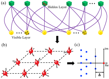
Figure 1: A sketch of the essential idea for accessing the Liouvillian gap with artificial neural networks. (a) The restricted Boltzmann machine (RBM) representation of quantum many-body density matrices under the “spin bi-base mapping”. (b) The dissipative spin-$1/2$ XYZ model defined on a 2D square lattice. (c) A pictorial sketch of the Liouvillian spectrum. The red dot corresponds to the non-equilibrium steady state with zero Liouvillian eigenvalue, whereas the blue dots on the vertical dotted line correspond to the first decay modes. $\Delta$ denotes the Liouvillian gap.

From the numerical computation point of view, computing the Liouvillian gap is a formidable task in general. In fact, it has been rigorously proved that the general spectral gap problem is undecidable even for closed quantum systems Lloyd (1993); Cubitt et al. (2015); Bausch et al. (2020): there exists no algorithm to determine whether an arbitrary Hamiltonian is gapped or not. Computing the Liouvillian gap is even harder in general. Fortunately, physical Hamiltonians or Liouvillians of practical interest often bear special structures, which may enable them to circumvent the undecidability and make their spectral gaps accessible by certain numerical methods. In particular, for solving Lindblad master equations to obtain the dynamics and non-equilibrium steady states of open quantum systems, a number of notable algorithms have been proposed Weimer et al. (2019), including matrix-product state and tensor network approaches Verstraete et al. (2004); Zwolak and Vidal (2004); Cai and Barthel (2013); Mascarenhas et al. (2015); Cui et al. (2015); Žnidarič (2015); Werner et al. (2016); Gangat et al. (2017); Kshetrimayum et al. (2017), corner-space renormalization Finazzi et al. (2015); Rota et al. (2019), cluster mean-field Jin et al. (2016), and quantum Monte Carlo Nagy and Savona (2018); Yan et al. (2018); Casteels et al. (2018). More recently, machine learning Goodfellow et al. (2016) approaches based on artificial neural networks have also been invoked to tackle this problem Hartmann and Carleo (2019); Vicentini et al. (2019); Nagy and Savona (2019); Yoshioka and Hamazaki (2019). The essential idea is to use neural network quantum states Carleo and Troyer (2017); Torlai and Melko (2018); Carrasquilla et al. (2019); Banchi et al. (2018); Cai and Liu (2018); Schmitt and Heyl (2020), especially the RBM states Carleo and Troyer (2017); Torlai and Melko (2018), to serve as ansatz density matrices for open quantum systems and adopt the stochastic reconfiguration (SR) method Sorella et al. (2007) to obtain their dynamics and steady states by solving the master equation variationally. Owing to the structure flexibility and long-range connections of neural networks, such approaches admit the striking merit of generic applicability to high dimensional systems with even volume-law entanglement Deng et al. (2017).

In this paper, we introduce a variational method based on the RBM representation to compute the Liouvillian gap. We use the “spin bi-base mapping” to map the density matrix to a pure state that is conveniently represented by RBMs. Under this mapping, the Liouvillian superoperator reduces to a rank-two non-Hermitian operator and the Liouvillian gap can be computed by the variational SR algorithm Sorella et al. (2007). To demonstrate and benchmark the accuracy and efficiency, we apply our method to the dissipative XYZ (also known as Heisenberg) models in both one and two dimensions (2D). We find that for the isotropic case (the dissipative XXZ model), the Liouvillian gap is always equal to half of the dissipation rate, independent of the coupling strengths, system sizes, and lattice geometry. Inspired by this observation, we show that for the dissipative XXZ model the Liouvillian gap is indeed exactly solvable, although the Liouvillian spectrum is not solvable in general. In 1D, we show that the whole Liouvillian spectrum can be exactly solved using the Bethe ansatz method. These analytic results may be of independent interest. For the anisotropic case, we compare our RBM results with the results from exact diagonalization (ED) and find that they match within a desirable accuracy.

The Liouvillian gap and RBM approach.—We consider the following Lindblad master equation Breuer and Petruccione (2007); Lidar (2019):

$$\frac{\mathrm{d}\rho}{\mathrm{d}t}=-i[H,\rho]+\sum_{\mu}(2L_{\mu}\rho L_{\mu}^{\dagger}-\{L_{\mu}^{\dagger}L_{\mu},\rho\})\equiv\mathcal{L}\rho,$$ (1)

where $\rho$ denotes the density matrix, $H$ is the Hamiltonian governing the unitary part of the dynamics, $L_{\mu}$ are the jump operators describing the dissipative process, the curly bracket represents the anticommutator, and $\mathcal{L}$ is the Liouvillian superoperator. In general, the index $\mu$ runs over all dissipation channels. For simplicity and concreteness, here we focus on the case where each lattice site has only one dissipation channel and $\mu$ just labels the lattice site. The generalization to the cases with multiple dissipation channels is straightforward.

The full spectrum of the Liouvillian superoperator $\mathcal{L}$ can be determined by solving the eigenequation: $\mathcal{L}\rho_{k}=\lambda_{k}\rho_{k}$, where $\lambda_{k}$ is the eigenvalue and $\rho_{k}$ denotes its corresponding eigenmatrix. Unlike the case of closed quantum systems, the eigenvalues of $\mathcal{L}$ are usually complex and their corresponding eigenmatrices are not necessarily physical (i.e., being Hermitian, trace-one, and semi-positive definite). Moreover, it can be proved Breuer and Petruccione (2007) that $\text{Re}(\lambda_{k})\leq 0$ for all $k$. For convenience, we sort the eigenvalues by their real parts in decreasing order [$\text{Re}(\lambda_{0})\geq\text{Re}(\lambda_{1})\geq\cdots$] with the steady state corresponding to $\lambda_{0}=0$ (for simplicity, we only focus on the case that the steady state is unique and $\lambda_{0}$ has no degeneracy). With this convention, the Liouvillian gap is defined as

$$\Delta=-\text{Re}(\lambda_{1}).$$ (2)

The Liouvillian gap is a central and fundamental physical quantity in studying open quantum systems. It determines the relaxation time from an arbitrary initial state to the steady state and plays a crucial role in characterizing dissipative phase transitions Rossatto and Villas-Boas (2016); Kessler et al. (2012); Minganti et al. (2018) and the exotic chiral damping phenomenon Song et al. (2019). Yet, for quantum many-body systems the dimension of the Liouville space scales double exponentially with the system size, rendering the computation of Liouvillian gap notably challenging.

We employ a spin bi-base mapping, which is also called the Choi-Jamiołkowski isomorphism Zwolak and Vidal (2004); Kshetrimayum et al. (2017), to map a density matrix to a vector in the computational bases:

$$\rho=\sum_{m,n}\rho_{mn}|m\rangle\langle n|\quad\Leftrightarrow\quad\tilde{\rho}=\sum_{m,n}\rho_{mn}|m\rangle\otimes|n\rangle.$$ (3)

Under this mapping, the Liouvillian superoperator $\mathcal{L}$, originally a rank-four tensor, reduces to a rank-two operator $\tilde{\mathcal{L}}=-iH\otimes I+iI\otimes H^{T}+\sum_{\mu}(2L_{\mu}\otimes L_{\mu}^{*}-L_{\mu}^{\dagger}L_{\mu}\otimes I-I\otimes L_{\mu}^{T}L_{\mu}^{*})$, where $I$ denotes the identity matrix and $T$ means the matrix transpose. We consider an open quantum system with $N$ qubits and use a RBM to describe $\tilde{\rho}$ with Carleo and Troyer (2017)

$$(\rho_{\text{RBM}})_{mn}=\exp{\left[\sum_{j=1}^{N}(a_{j}\sigma_{j,R}^{z}+b_{j}\sigma_{j,L}^{z})\right]}\prod_{k=1}^{M}X_{k},$$ (4)

where $\sigma^{z}_{j,R(L)}=\pm 1$ denotes the visible neurons responsible for the $|m\rangle=|\sigma^{z}_{1,R},\cdots,\sigma^{z}_{N,R}\rangle$ $\left(|n\rangle=|\sigma^{z}_{1,L},\cdots,\sigma^{z}_{N,L}\rangle\right)$ part of $\tilde{\rho}$. $M$ is the number of hidden neurons, and $X_{k}=\cosh\left(c_{k}+\sum_{j}W^{R}_{k,j}\sigma_{j,R}^{z}+\sum_{j}W^{L}_{k,j}\sigma_{j,L}^{z}\right)$. Here, $\{a_{j},b_{j},c_{k}\}$ are on-site weight parameters, and $\{W^{R}_{k,j}$, $W^{L}_{k,j}\}$ are connection parameters between visible and hidden neurons. We note that the matrix $\rho$ corresponding to $\tilde{\rho}$ may not be physical, in contrast to the representations of density matrices introduced in Refs. Torlai and Melko (2018); Hartmann and Carleo (2019); Vicentini et al. (2019); Nagy and Savona (2019); Yoshioka and Hamazaki (2019). This is not a problem for our purpose because here we mainly focus on the eigenmatrices of $\mathcal{L}$, which are not physical in general.

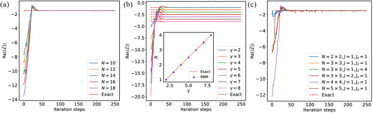
Figure 2: Numerical results for the dissipative XXZ model in one [(a) and (b)] and two [(c)] dimensions. (a) The real part of the expectation value $\text{Re}(\langle\tilde{\mathcal{L}}\rangle)=\text{Re}(\langle\rho^{\prime}|\tilde{\mathcal{L}}|\rho^{\prime}\rangle/\langle\rho^{\prime}|\rho^{\prime}\rangle)$ as a function of the iteration steps for different lattice sizes $N$. The parameters are chosen as $J_{x}=J_{y}=1$, $J_{z}=2$, and $\gamma=3$. The red dashed horizontal line indicates the exact value of the Liouvillian gap $\Delta$ obtained by exact diagonalization, which can also be derived analytically (see the main text). (b) $\text{Re}(\langle\tilde{\mathcal{L}}\rangle)$ as a function of iteration steps for different dissipation rates. Here, $J_{x}=J_{y}=1$, $J_{z}=2$, and $N=10$. The inset shows the linear dependence of the Liouvillian gap obtained by the RBM method on the dissipation rate $\gamma$. (c) $\text{Re}(\langle\hat{\mathcal{L}}\rangle)$ for 2D dissipative XXZ model with $\gamma=3$, and varying lattice sizes and coupling strengths (see LGv for details).

Given the RBM parametrization of $\tilde{\rho}$, we can now recast the problem of computing the Liouvillian gap as a variational optimization problem in a subspace orthogonal to the steady state $\rho_{0}$. Yet, the subtraction of $\rho_{0}$ is tricky. Analogous to the closed system case, one may regard the first decay modes as the first “excited states” of $\mathcal{L}$ and then the Liouvillian gap is just the “first excited energy”. Consequently, a possible way to obtain the Liouvillian gap is by first computing the steady state of $\mathcal{L}$ and then appropriately extending the protocols for calculating the excited states of closed systems Vieijra et al. (2020); Choo et al. (2018) to open systems. This approach is straightforward, yet technically cumbersome. By noticing the fact that $\mathcal{L^{\dagger}}I=0$, $\text{Tr}(\mathcal{L}\rho_{k})=0=\lambda_{k}\text{Tr}(\rho_{k})$ and hence $\text{Tr}(\rho_{k})=0$ for all $\lambda_{k}\neq 0$, a much simpler approach is to construct a new variational matrix $\rho^{\prime}$ with vanishing trace

$$\rho^{\prime}=\alpha\rho^{\prime}_{0}+\rho_{\text{RBM}},$$ (5)

where $\alpha=-\frac{\text{Tr}(\rho_{\text{RBM}})}{\text{Tr}(\rho^{\prime}_{0})}$, $\rho^{\prime}_{0}$ is a density matrix with nonzero trace which is not necessary the true steady state, and $\rho_{\text{RBM}}$ is a RBM ansatz state as defined in Eq. (4). Since $\text{Tr}(\rho^{\prime})=0$, $\rho^{\prime}$ lives in the subspace orthogonal to $\rho_{0}$. We adapt the SR method Sorella et al. (2007) to generate the real time evolution of $\rho^{\prime}$ LGv . Unlike the case for closed systems, $\tilde{\mathcal{L}}$ is not Hermitian and its right eigenvectors are not orthogonal in general. This non-Hermiticity makes the problem more complicated. Three different cases arise based on the properties of the first decay modes: (i) there is only one first decay mode, then $\rho^{\prime}\rightarrow\rho_{1}$ after long enough real-time evolution and the Liouvillian gap can be obtained by $\Delta=-\text{Re}(\langle\rho^{\prime}|\mathcal{L}|\rho^{\prime}\rangle/\langle\rho^{\prime}|\rho^{\prime}\rangle)$; (ii) there are multiple first decay modes but they are orthogonal to each other, then $\rho^{\prime}$ will converge to a superposition of these decay modes and $\Delta$ can still be obtained in the same way as in the first case; (iii) there exist multiple first decay modes [denoted as $\rho_{1}^{(1)},\rho_{1}^{(2)},\rho_{1}^{(3)},\cdots$] which are not orthogonal. In this case, $\rho^{\prime}$ will converge to a superposition of these decay modes: $\rho^{\prime}\rightarrow a_{1}\rho_{1}^{(1)}+a_{2}\rho_{1}^{(2)}+a_{3}\rho_{1}^{(3)}+\cdots$, where $a_{1},a_{2},a_{3},\cdots$ are coefficients whose values depend on the initialization of $\rho^{\prime}$. Due to the non-orthogonality, $\langle\rho_{1}^{(i)}|\mathcal{L}|\rho_{1}^{(j)}\rangle\neq 0$ for $i\neq j$ and $\Delta\neq-\text{Re}(\langle\rho^{\prime}|\mathcal{L}|\rho^{\prime}\rangle/\langle\rho^{\prime}|\rho^{\prime}\rangle)$ at this stage in general. To overcome this problem, we should add another imaginary time evolution for $\rho^{\prime}$ under $i\mathcal{L}$ with a smaller learning rate so that it converges further to the first decay mode with the minimal imaginary part. After this modification, $\Delta$ can be obtained again by computing $-\text{Re}(\langle\rho^{\prime}|\mathcal{L}|\rho^{\prime}\rangle/\langle\rho^{\prime}|\rho^{\prime}\rangle)$ LGv . We stress the fact that the non-Hermiticity of $\mathcal{L}$ makes the computation of the Liouvillian gap much subtler than computing the energy gap for a Hermitian Hamiltonian, as discussed above. However, the computational complexity of our RBM approach does not increase too much and is still favorable LGv .

Concrete examples.—We consider the dissipative spin-1/2 XYZ model, where each spin has a Heisenberg type interaction with its nearest neighboring spins and is subject to a dissipation process into the $|S^{z}=-1/2\rangle$ state:

$$\frac{d\rho}{dt}=-i[H,\rho]+\frac{\gamma}{2}\sum_{j}[2S_{j}^{-}\rho S_{j}^{+}-\{S_{j}^{+}S_{j}^{-},\rho\}].$$ (6)

Here $H=\sum_{\langle j,k\rangle}\left(J_{x}S_{j}^{x}S_{k}^{x}+J_{y}S_{j}^{y}S_{k}^{y}+J_{z}S_{j}^{z}S_{k}^{z}\right)$, $S^{\mu}=\frac{1}{2}\sigma^{\mu}$ with $\sigma^{\mu}$ being the Pauli matrix ($\mu=x,y,z$), $J_{\mu}$ denotes the coupling constant between nearest neighboring spins, and $S^{\pm}=S^{x}\pm iS^{y}$. The dynamics and steady state properties of this dissipative XYZ model have already been widely studied Jin et al. (2016); Lee et al. (2013a); Rota et al. (2017, 2018); Casteels et al. (2018); Huybrechts and Wouters (2019); Hartmann and Carleo (2019); Nagy and Savona (2019). In particular, in 2D it exhibits a dissipative phase transition between a paramagnetic and a ferromagnetic phase Jin et al. (2016); Lee et al. (2013a); Rota et al. (2017, 2018); Casteels et al. (2018); Huybrechts and Wouters (2019), which originates from the competition between the unitary evolution and the incoherent dynamics. Different from the previous works that mainly focus on dynamics or steady state properties, here we focus on the computation of the Liouvillian gap instead.

We apply the introduced RBM approach to compute the Liouvillian gap for the dissipative XYZ model in both one and two dimensions. For the isotropic case $J_{x}=J_{y}=J$, the XYZ model reduces to the XXZ model and our numerical results are shown in Fig. 2. From this figure, it is evident that the real part of the expectation value $\text{Re}(\langle\tilde{\mathcal{L}}\rangle)=\text{Re}(\langle\rho^{\prime}|\tilde{\mathcal{L}}|\rho^{\prime}\rangle/\langle\rho^{\prime}|\rho^{\prime}\rangle)$ converges quickly to the exact value of the Liouvillian gap, validating the effectiveness of the RBM method. To measure the accuracy, we define the relative error $\epsilon_{\text{rel}}=|(\Delta_{\text{RBM}}-\Delta_{\text{Ex}})/\Delta_{\text{Ex}}|$ and find that $\epsilon_{\text{rel}}\approx 10^{-2}$ after around $50$ iteration steps for all the scenarios shown in Fig. 2. We mention that the accuracy can be systematically improved by increasing the number of hidden neurons or the length of the Markov chain used in the SR algorithm LGv .

An interesting observation from our RBM results shown in Fig. 2 is that for the dissipative XXZ model, the Liouvillian gap is always equal to half of the dissipation rate $\Delta=\gamma/2$, independent of the coupling strengths $J$ and $J_{z}$, system size, boundary condition, and the model dimensionality. This inspired us to suspect that the Liouvillian gap is exactly solvable owing to special structures of the dissipative XXZ model. Indeed, we find that $\Delta$ can be analytically derived as below. After the spin bi-base mapping, the Liouvillian superoperator $\mathcal{L}$ for the dissipative XXZ model is mapped to: $\tilde{\mathcal{L}}=-i\sum_{\langle i,j\rangle}[J_{z}(S_{i,R}^{z}S_{j,R}^{z}-S_{i,L}^{z}S_{j,L}^{z})+\frac{1}{2}J(S_{i,R}^{+}S_{j,R}^{-}+S_{i,R}^{-}S_{j,R}^{+}-S_{i,L}^{+}S_{j,L}^{-}-S_{i,L}^{-}S_{j,L}^{+})]+\frac{\gamma}{2}\sum_{i}(2S_{i,R}^{-}S_{i,L}^{-}-S_{i,R}^{z}-S_{i,L}^{z}-1)$. One may regard $\tilde{\mathcal{L}}$ as a non-Hermitian Hamiltonian for two copies of the original dissipative system, with one copy corresponding to the right ket (the $|m\rangle$ part) and the other copy corresponding to the left bra (the $|n\rangle$ part) in Eq. (3). We then rearrange the terms in $\tilde{\mathcal{L}}$ accordingly:

$$\tilde{\mathcal{L}}=H_{R}+H_{L}+\gamma\sum_{i}D_{i},$$ (7)

where $D_{i}=S_{i,R}^{-}S_{i,L}^{-}$ describes the couplings between the left and right spins, and $H_{R}=-i\sum_{\langle i,j\rangle}[J(S_{i,R}^{+}S_{j,R}^{-}+S_{i,R}^{-}S_{j,R}^{+})+J_{z}S_{i,R}^{z}S_{j,R}^{z}]-\frac{\gamma}{2}\sum_{i}(S^{z}_{i,R}+\frac{1}{2})$ and $H_{L}=i\sum_{\langle i,j\rangle}[J(S_{i,L}^{+}S_{j,L}^{-}+S_{i,L}^{-}S_{j,L}^{+})+J_{z}S_{i,L}^{z}S_{j,L}^{z}]-\frac{\gamma}{2}\sum_{i}(S^{z}_{i,L}+\frac{1}{2})$ denote the Hamiltonians for the right and left subsystems, respectively. It is easy to observe that $[H_{L},H_{R}]=0$ since they belong to different subsystems, and both $H_{L}$ and $H_{R}$ have a $U(1)$ symmetry, namely their total $S^{z}$ is conserved respectively. Consequently, $\tilde{\mathcal{L}^{\prime}}=H_{R}+H_{L}$ can be block-diagonalized with each block maintaining a fixed total $S^{z}$. Following Ref. Torres (2014), in the bases where $\tilde{\mathcal{L}^{\prime}}$ is block-diagonal, each term $D_{i}$ is just an upper triangular matrix with vanishing diagonal terms, thus adding these terms will only alter the eigenstates but not the eigenvalues of $\tilde{\mathcal{L}^{\prime}}$. The eigenspectrum of $\tilde{\mathcal{L}}$ is exactly the same as $\tilde{\mathcal{L}^{\prime}}$ LGv . In addition, it is easy to observe that the steady state of $\mathcal{L}$ is the state with all spins pointing down due to the dissipation process. Noting that $\tilde{\mathcal{L}}^{\prime}$ contains only imaginary XXZ interactions and a magnetic field with strength $\frac{\gamma}{2}$, hence the real part of the spectrum of $\tilde{\mathcal{L}}$ is just $-\frac{\gamma}{2}m$, where $m$ denotes the number of “magnons” created from the steady state (the number of spins flipped from down to up). As a result, the desired Liouvillian gap corresponds to a single-magnon excitation, which leads to $\Delta=\frac{\gamma}{2}$, independent of $J,J_{z}$, system size, and lattice geometry. In 1D with periodic boundary condition, the whole Liouvillian spectrum can be deduced from the Bethe ansatz solution LGv :

$$E(\{k_{j}\}_{m})=-\frac{\gamma}{2}m\pm i\sum_{j=1}^{m}(2J\textnormal{cos}k_{j}-J_{z}).$$ (8)

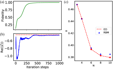
Figure 3: Numerical results for the dissipative XYZ model in 1D. (a) and (b) show respectively the fidelity between $|\rho^{\prime}\rangle$ and $|\rho_{1}\rangle$, and the expectation value $\text{Re}(\langle\tilde{\mathcal{L}}\rangle)$, as functions of the iteration steps for $N=4$. After around 500 iterations, $\text{Re}(\langle\tilde{\mathcal{L}}\rangle)$ converges to the exact value of the Liouvillian gap $\Delta$ [indicated by the red dashed line in (b)] with relative error $\epsilon_{\text{rel}}\approx 10^{-2}$ and the fidelity approaches one ($|\langle\rho^{\prime}|\rho_{1}\rangle|\approx 0.991$). (c) The comparison between the RBM and ED results with varying system sizes. Here, the model parameters are chosen as $J_{x}=4$, $J_{y}=0.5$, $J_{z}=2$, and $\gamma=1$ LGv .

We now turn to the anisotropic case with $J_{x}\neq J_{y}$, where the Liouvillian gap cannot be solved analytically in general. Our numerical results are shown in Fig. 3. From this figure, it is clear that our RBM results match the exact results from exact diagonalization within a reasonable accuracy. We note that, in Fig. 3(c), the apparent deviation of the RBM result for $N=10$ from its exact value is due to the small plotting range. A closer examination shows that for this point, the relative error is $\epsilon_{\text{rel}}=1.46\times 10^{-2}$ in fact. In comparison with the case of the XXZ model, we find that the convergence for the XYZ model is notably slower. The reason for this is that for the XXZ model, its multiple first decay modes are orthogonal to each other. Hence, to obtain $\Delta$, $\rho^{\prime}$ only needs to converge to a subspace spanned by these modes. Whereas for the XYZ model, depending on the parameters there exist either only one or multiple but non-orthogonal first decay modes LGv . Thus, as discussed previously, to obtain $\Delta$ accurately in this case, $\rho^{\prime}$ needs to converge to a single decay mode, which demands extra iteration steps and possibly more hidden neurons to increase the representation power. We note that our RBM approach may also carry over straightforwardly to systems with higher spins, interacting bosons Saito (2017); Choo et al. (2018) and fermions Nomura et al. (2017); Choo et al. (2020), or models with long-range interactions Deng et al. (2017); LGv .

Discussion and conclusion.— We mention that the general spectral gap problem has been mathematically proved to be an undecidable problem Lloyd (1993); Cubitt et al. (2015); Bausch et al. (2020) from the computational complexity perspective Arora and Barak (2009), implying that there exists no algorithm to determine whether an arbitrary model is gapped or gapless. As a result, we cannot expect that our RBM approach could solve the Liouvillian gap for all possible Liouvillian superoperators. In fact, no algorithm is capable of doing this due to the undecidability of the problem. Finding out the key properties of the Liouvillian superoperators that warrant the effectiveness of the RBM approach is of both fundamental and practical importance. Yet, this may require new physical concepts and a deeper understanding of artificial neural networks, similar to the case of how we understand the effectiveness of the density-matrix-renormalization-group algorithm Schollwöck (2005) from the entanglement perspective. In addition, one may also use other neural networks, such as deep Boltzmann machine Gao and Duan (2017) or feedforward neural networks Cai and Liu (2018), to compute the the Liouvillian gap. More recently, a quantum-classical hybrid algorithm based on deep quantum neural networks has also been introduced to solve the steady states and dynamics for open systems Liu et al. (2020). It would also be interesting to extend this approach to compute the Liouvillian gap through noisy intermediate-scale quantum devices Preskill (2018).

In summary, we have introduced a machine learning based approach to compute the Liouvillian gap for open quantum systems, which is generally applicable to high dimensional systems with massive entanglement. The accuracy and effectiveness of this approach have been benchmarked with numerical examples for the dissipative Heisenberg model in both one and two dimensions. Based on the numerical results, we found that the Liouvillian gap is exactly solvable for the dissipative XXZ model regardless of the system size and lattice geometry. These analytic results are of independent interest as well and may inspire subsequent analytical studies.

We acknowledge helpful discussions with Fei Song, Shunyao Zhang and computational resources provided by Yiyang Wu and Benda Xu. This work was supported by the start-up fund from Tsinghua University (Grant No. 53330300320), NSFC under Grants No. 11674189 and 12075128, and the Shanghai Qi Zhi Institute.

Note added.— After this work was finished, we became aware of a recent work Buča et al. (2020), which also analytically studied the Liouvillian spectrum based on the Bethe ansatz method.

Supplementary Material for: Solving the Liouvillian Gap with Artificial Neural Networks

I The stochastic reconfiguration algorithm

As mentioned in the main text, we adopt the stochastic reconfiguration (SR) method Sorella et al. (2007); Carleo and Troyer (2017); Choo et al. (2018) to generate the real time evolution of the ansatz density matrix $\rho^{\prime}$. We note that for closed quantum systems, this kind of variational optimization can be achieved equivalently by the standard stochastic gradient descent (SGD) or imaginary time evolution (via SR). However, due to the non-Hermiticity of Liouvillian superoperator $\mathcal{L}$, the orthogonality of right eigenstates is lost. The extreme value of $\text{Re}(\langle\mathcal{L}\rangle)$, which is usually used as the cost function, generally will not correspond to the Liouvillian gap $\Delta$. The appearance of crossing terms like $\langle\rho_{i}|\rho_{j}\rangle\ (\{|\rho_{i}\rangle\}\text{ are right eigenstates of }\mathcal{L},\ i\neq j)$ will lead to the failure of the former method for open quantum systems. This property can be clearly observed from Fig. 2 of the main text, where during the converging process, $\text{Re}(\langle\mathcal{L}\rangle)$ has once exceeded the value of $-\Delta$.

In the framework of SR, given a variational ansatz $|\rho^{\prime}(\{\alpha_{k}\})\rangle$, where $\{\alpha_{k}\}$ stand for the real-number variational parameters like $\{a_{j},b_{j},c_{k},W_{j,k}^{R(L)}\}$ in the RBM, we need to optimize $\{\alpha_{k}\}$ such that the trial bi-base wavefunction will finally converge to the first decay modes. First we define the logarithmic derivative operator for each parameter $\alpha_{k}$ as $O_{k}$. Note that $O_{k}$ is diagonal under computational bi-bases $\{|x\rangle=|\sigma_{1,R}^{z},\sigma_{2,R}^{z},\cdots,\sigma_{N,R}^{z},\sigma_{1,L}^{z},\sigma_{2,L}^{z},\cdots,\sigma_{N,L}^{z}\rangle\}$:

$$\langle x^{\prime}|O_{k}|x\rangle=\delta_{x^{\prime}x}\partial_{k}\ln\langle x|\rho^{\prime}(\{\alpha_{k}\})\rangle.$$ (S1)

Consider a small change $\{\delta\alpha_{k}\}$ on the parameters with respect to the initial values $\{\alpha_{k}^{0}\}$

$$\alpha_{k}=\alpha_{k}^{0}+\delta\alpha_{k}.$$ (S2)

The corresponding bi-base wavefunction will deviate from the original term $|\rho^{\prime 0}\rangle$ by

$$|\rho^{\prime}\rangle=|\rho^{\prime 0}\rangle+\sum_{k}\delta\alpha_{k}O_{k}|\rho^{\prime 0}\rangle.$$ (S3)

The stochastic reconfiguration scheme proceeds by performing a series of infinitesimal real time evolution governed by the Liouvillian superoperator $\mathcal{L}$, which up to the first order of learning rate $\epsilon$ is given by

$$|\rho^{\prime}_{\text{e(xact)}}\rangle=e^{\epsilon\mathcal{L}}|\rho^{\prime 0}\rangle\approx(1+\epsilon\mathcal{L})|\rho^{\prime 0}\rangle.$$ (S4)

Now we want to find out the optimal updated parameters $\{\alpha_{k}\}$ to maximize the overlap between $|\rho^{\prime}\rangle$ and $|\rho^{\prime}_{e}\rangle$. This maximization is equivalent to requiring

$$\langle\rho^{\prime}_{e}|\rho^{\prime}\rangle\langle\rho^{\prime}|\rho^{\prime}_{e}\rangle=\langle\rho^{\prime}_{e}|\rho^{\prime}_{e}\rangle\langle\rho^{\prime}|\rho^{\prime}\rangle,$$ (S5)

after some algebraic operations and dropping high-order terms like $\epsilon^{2}$ or $\epsilon\delta\alpha\delta\alpha$, we obtain the linear equation

$$\sum_{k^{\prime}}\left(\langle O_{k}^{\dagger}O_{k^{\prime}}\rangle+\langle O_{k^{\prime}}^{\dagger}O_{k}\rangle-\langle O_{k}^{\dagger}\rangle\langle O_{k^{\prime}}\rangle-\langle O_{k^{\prime}}^{\dagger}\rangle\langle O_{k}\rangle\right)\delta\alpha_{k^{\prime}}$$

$$=\epsilon\left(\langle\mathcal{L}^{\dagger}O_{k}\rangle+\langle O_{k}^{\dagger}\mathcal{L}\rangle-\langle\mathcal{L}^{\dagger}\rangle\langle O_{k}\rangle-\langle O_{k}^{\dagger}\rangle\langle\mathcal{L}\rangle\right)$$ (S6)

where $\langle\cdot\rangle$ denotes the average on the state $|\rho^{\prime 0}\rangle$.

In short Eq. (S6) can be written as $\sum_{k^{\prime}}S_{kk^{\prime}}\delta\alpha_{k^{\prime}}=\epsilon F_{k}$, where $S$ and $F$ are usually called the covariance matrix and force. Finally by solving this linear equation the updated parameter vector can be computed as $\delta\alpha=\epsilon S^{-1}F$. Usually a regularization on $S$ Carleo and Troyer (2017); Choo et al. (2018) will be applied to decrease the fluctuation error generated in the Monte Carlo process that will be discussed in the next section:

$$\widetilde{S}=S+\lambda I\quad\lambda\in[10^{-4},10^{-2}].$$ (S7)

We continuously repeat the iteration above to update the parameters until convergence.

Besides, for the case (iii) of first decay modes mentioned in the main text, in order to make the RBM ansatz further converge to the first decay mode with the minimal imaginary part, we should add another imaginary time evolution for $\rho^{\prime}$ under $i\mathcal{L}$ with smaller learning rate $\beta\epsilon$. Hence, another force $F^{\prime}$ will be added

$$F_{k}^{\prime}=-i\langle\mathcal{L}^{\dagger}O_{k}\rangle+i\langle O_{k}^{\dagger}\mathcal{L}\rangle+i\langle\mathcal{L}^{\dagger}\rangle\langle O_{k}\rangle-i\langle O_{k}^{\dagger}\rangle\langle\mathcal{L}\rangle,$$ (S8)

and the linear equation becomes

$$\sum_{k^{\prime}}S_{kk^{\prime}}\delta\alpha_{k^{\prime}}=\epsilon(F_{k}+\beta F_{k}^{\prime})\quad\beta\in[10^{-3},10^{-2}].$$ (S9)

Under the joint evolution of $\mathcal{L}+i\beta\mathcal{L}$,

$$\rho^{\prime} =e^{(\mathcal{L}+i\beta\mathcal{L})t}\rho^{\prime 0}$$

$$=c_{0}\rho_{0}+\sum_{i\neq 0}c_{i}e^{(\lambda_{i}+i\beta\lambda_{i})t}\rho_{i}\quad(c_{0}=0)$$

$$=\sum_{i\neq 0}c_{i}e^{(\text{Re}(\lambda_{i})-\beta\text{Im}(\lambda_{i}))t}e^{i(\text{Im}(\lambda_{i})+\beta\text{Re}(\lambda_{i}))t}\rho_{i},$$ (S10)

where $\rho_{0}$ denotes the steady state and $\{\rho_{i}\}_{i\neq 0}$ are other decay eigenmodes. After long enough time, clearly $\rho^{\prime}$ will converge to the first decay mode with the minimal imaginary part. A numerical example belonging to this case will be shown in the last section.

II The Markov chain Monte Carlo

In order to efficiently compute the average of observables mentioned in the previous section, we introduce the standard Markov chain Monte Carlo (MCMC) method as follows. Given an observable $\hat{B}$ (like $O_{k}$ and $\mathcal{L}$), we convert its average into the stochastic form:

$$\langle\hat{B}\rangle =\frac{\langle\rho^{\prime}|\hat{B}|\rho^{\prime}\rangle}{\langle\rho^{\prime}|\rho^{\prime}\rangle}$$

$$=\sum_{x,x^{\prime}}\frac{\langle\rho^{\prime}|x\rangle\langle x|\hat{B}|x^{\prime}\rangle\langle x^{\prime}|\rho^{\prime}\rangle}{\langle\rho^{\prime}|\rho^{\prime}\rangle}$$

$$=\sum_{x,x^{\prime}}\frac{\langle\rho^{\prime}|x\rangle\langle x|\rho^{\prime}\rangle}{\langle\rho^{\prime}|\rho^{\prime}\rangle}\frac{\langle x|\hat{B}|x^{\prime}\rangle\langle x^{\prime}|\rho^{\prime}\rangle}{\langle x|\rho^{\prime}\rangle}$$

$$=\mathbb{E}\left(\sum_{x^{\prime}}\frac{\langle x|\hat{B}|x^{\prime}\rangle\langle x^{\prime}|\rho^{\prime}\rangle}{\langle x|\rho^{\prime}\rangle}\right)\quad\text{by sampling a distribution }|\langle x|\rho^{\prime}\rangle|^{2}.$$ (S11)

Since $O_{k}$ is diagonal under computational bi-bases, the explicit expressions of $O_{k}$ for the RBM ansatz can be directly read out as follows:

$$O_{\text{Re}(a_{j})}=\sigma_{j,R}^{z}\quad O_{\text{Im}(a_{j})}=i\sigma_{j,R}^{z}\quad O_{\text{Re}(b_{j})}=\sigma_{j,L}^{z}\quad O_{\text{Im}(b_{j})}=i\sigma_{j,L}^{z},$$ (S12)

$$O_{\text{Re}(c_{k})}=\tanh{X_{k}}\quad O_{\text{Im}(c_{k})}=i\tanh{X_{k}},$$ (S13)

$$O_{\text{Re}(W_{k,j}^{R(L)})}=\sigma_{j,R(L)}^{z}\tanh{X_{k}}\quad O_{\text{Im}(W_{k,j}^{R(L)})}=i\sigma_{j,R(L)}^{z}\tanh{X_{k}}.$$ (S14)

For achieving the stochastic average, we will generate a Markov chain of computational bi-bases $x_{1}\rightarrow x_{2}\rightarrow x_{3}\rightarrow\cdots\rightarrow x_{N_{s}}$ with total length $N_{s}$ by sampling $|\rho^{\prime}|^{2}$. This process can be realized by the well-known Metropolis-Hasting algorithm Metropolis et al. (1953): At step $i$, we randomly flip 1 to 4 spins in $x_{i}$ to obtain a new sample and calculate the following acceptance probability to determine whether to accept it:

$$A(x_{i}\rightarrow x_{i+1})=\min\left(1,\left|\frac{\rho_{x_{i+1}}}{\rho_{x_{i}}}\right|^{2}\right).$$ (S15)

Then we use the ensemble observable average of the Markov chain to estimate the stochastic average. Besides, considering the thermalization process, we need to drop the first $5\%$ of the Markov chain.

After each SR iteration, we should recompute the trace of updated RBM ansatz $\rho_{\text{RBM}}$ in order to make sure $\textnormal{Tr}(\rho^{\prime})=0$, as mentioned in the main text. This step can be achieved directly in small system size (typically $N\leq 10$) and also can be implemented by a sampling paradigm for larger system size as follows.

$$\frac{\textnormal{Tr}(\rho_{\text{RBM}})}{\textnormal{Tr}(\rho_{0}^{\prime})} =\frac{\langle I|\rho_{\text{RBM}}\rangle}{\langle I|\rho_{0}^{\prime}\rangle}\qquad(|I\rangle=\sum_{l=0}^{2^{N}-1}|l,l\rangle\text{ which is the bi-base state corresponding to the identity matrix})$$

$$=\sum_{l=0}^{2^{N}-1}\frac{\langle I|l,l\rangle\langle l,l|\rho_{\text{RBM}}\rangle}{\langle I|\rho_{0}^{\prime}\rangle}$$

$$=\sum_{l=0}^{2^{N}-1}\frac{\langle I|l,l\rangle\langle l,l|\rho_{0}^{\prime}\rangle}{\langle I|\rho_{0}^{\prime}\rangle}\frac{\langle l,l|\rho_{\text{RBM}}\rangle}{\langle l,l|\rho_{0}^{\prime}\rangle}$$

$$=\mathbb{E}\left(\frac{\langle l,l|\rho_{\text{RBM}}\rangle}{\langle l,l|\rho_{0}^{\prime}\rangle}\right)\quad\text{by sampling a distribution }p(l)\propto\langle l,l|\rho_{0}^{\prime}\rangle\text{ on }l\ (l=0,1\cdots,2^{N}-1)$$ (S16)

The diagonal real ancillary $\rho_{0}^{\prime}$ should be chosen appropriately according to the specific Liouvillian $\mathcal{L}$, mainly resembling its steady state property. For example, $\rho_{0}^{\prime}$ for the 1D/2D XXZ model corresponds to the bi-base state with all spins pointing down, so that we can impose $\rho_{\text{RBM}}(0,0)=\textnormal{Tr}(\rho_{\text{RBM}})$, whereas $\rho_{0}^{\prime}$ used for the XYZ model is the identity matrix. Besides, in order to obtain better convergence performance, the derivative of $\textnormal{Tr}(\rho_{\text{RBM}})$ can also be taken into consideration similarly.

$$\partial_{k}\frac{\textnormal{Tr}(\rho_{\text{RBM}})}{\textnormal{Tr}(\rho_{0}^{\prime})}=\partial_{k}\frac{\langle I|\rho_{\text{RBM}}\rangle}{\langle I|\rho_{0}^{\prime}\rangle}=\mathbb{E}\left(O_{k}(l,l)\frac{\langle l,l|\rho_{\text{RBM}}\rangle}{\langle l,l|\rho_{0}^{\prime}\rangle}\right)$$

$$\text{by sampling a distribution }p(l)\propto\langle l,l|\rho_{0}^{\prime}\rangle\text{ on }l\ (l=0,1\cdots,2^{N}-1)$$ (S17)

In our numerical calculations, the typical sampling size $N_{s}$ is 2 to 5 times as many as the variational parameters. The ratio between hidden neurons and visible neurons $M/2N$ is around 3 to 6. The learning rate is given by $\epsilon=\max(0.01,0.1\times 0.96^{p}),\beta=0.005\sim 0.05$ ($p$ is the iteration step). The regularization parameter takes $\lambda=\max(10^{-4},0.9^{p})$.

III Representation power of the RBM and computational cost

In this section, in order to make the article more self-contained and accessible to the general audience, we will provide a brief introduction for the representation power of the RBM ansatz and discuss about the computational cost. For an existing review of the RBM method, readers can refer to Melko et al. (2019).

As mentioned in the main text, owing to the structure flexibility and long-range connections of neural networks,the restricted Boltzmann machine (RBM) ansatz is able to represent quantum states with even volume-law entanglement in high dimensional systems Deng et al. (2017). The cases with volume-law entanglement, as expected, will appear more frequently in the open quantum systems. In contrast to the DMRG (density-matrix-renormalization-group) or other tensor-network approaches, entanglement is not a limiting factor for our RBM approach. Yet, it is also important to clarify that the RBM ansatz cannot represent all the volume-law entangled states efficiently. Indeed, it has been rigorously proven in Ref. Gao and Duan (2017) that there exist certain quantum states (which are generated either by polynomial-size quantum circuits or as ground states of certain gapped Hamiltonians) that cannot be represented by RBMs with a polynomial number of parameters, unless the polynomial hierarchy (a generalization of the famous P versus NP problem in computer science) collapses (which is widely believed to be unlikely).

Finding out the key properties of the Liouvillian superoperators that warrant the effectiveness of the RBM approach is of both fundamental and practical importance. However, this may require new physical concepts and a deeper understanding of artificial neural networks, similar to the case of how we understand the effectiveness of the DMRG algorithm from the entanglement perspective Schollwöck (2005). There are still many open questions about the representation power and effectiveness of the RBM method, which need further explorations in the future.

We also remark that our RBM approach may carry over straightforwardly to systems with higher spins, interacting bosons and fermions, or models with long-range interactions. In fact, for closed quantum systems the RBM method has been explored for bosons Saito (2017); Choo et al. (2018), fermions Nomura et al. (2017); Choo et al. (2020), and models with long-range interactions Deng et al. (2017). The general ideas are as follows. For higher spins or bosonic systems, we need to increase the degrees of freedom for the neurons in the RBM representation, whereas for fermionic systems, a Slater determinant or a pair-product wave function can be added to satisfy the Fermi-Dirac statistics. To demonstrate the effectiveness of our RBM approach in dealing with long-range interactions, we have also carried out numerical calculations for the Liouvillian gap of the dissipative long-range XXZ model and our results are plotted in Fig. S3.

As for the computational cost of the RBM method, the total complexity for each SR iteration is bounded by the MCMC sampling and the matrix inversion operation. For the first part, in the numerical calculation we usually take the Monte Carlo sampling size proportional to the number of variational parameters, $O(N_{\text{par}})$. According to Eqn. S6, the operation times to generate one covariance matrix $S$ are $O(N_{\text{par}}^{3})$. However, the sampling step can be significantly sped up by parallel processing (on CPU or GPU) and batch processing. Concretely, we do not update all the parameters in one SR iteration, but divide them up and update separately in parallel. For the matrix inversion part, $\delta\alpha=\epsilon S^{-1}F$, direct Gauss elimination will be bounded by the complexity of $O(N_{\text{par}}^{3})$. Yet, following the method mentioned in the Supplementary Material of Carleo and Troyer (2017), this cost can be reduced to $O(N_{\text{par}}^{2})$ by means of iterative solvers which never form the covariance matrix $S$ explicitly. Finally, the number of parameters $N_{\text{par}}$ depends on the specific structure of RBM ansatz. In most cases, each hidden neuron is coupled to all the visible neurons and the number of hidden neurons is usually on the same order of that for visible neurons, $M\sim N$, hence $N_{\text{par}}=O(M\times N)=O(N^{2})$. This number of variational parameters may be further reduced by exploiting the translational symmetry (see the last section for details) or the locality property (one hidden neuron only couples to nearest $O(1)$ visible neurons), which will lead to significant speed up in practice.

In summary, the total computational complexity for each SR iteration is upper bounded by a polynomial cost $O(N_{\text{par}}^{3})$, and many numerical techniques mentioned above can significantly reduce this complexity. In the generalization of RBM method to bosonic systems, fermionic systems or lattice models with long-range interactions, the total computational cost may increase a little bit due to the increase of the degrees of freedom of the neurons or the extra Slater determinant. However, in all the cases the complexity still scales polynomially with the system size $N$ and many numerical tricks have been developed and adopted to speed up the computation process.

IV Eigenstates of the dissipative XXZ model

As mentioned in the main text, the Liouvillian spectrum of dissipative XXZ model coincides with that of $\tilde{\mathcal{L}}^{\prime}=H_{R}+H_{L}$, but not for the eigenstates. In this section we will give the general conditions for this kind of coincidence, and demonstrate how to construct the eigenstates of $\mathcal{L}$ from that of $\tilde{\mathcal{L}}^{\prime}$ by following calculations in Torres (2014).

A Liouvillian superoperator $\mathcal{L}$, in the representation of Choi-Jamiołkowski isomorphism Zwolak and Vidal (2004); Kshetrimayum et al. (2017) can always be decomposed into three parts:

$$\tilde{L}=(-iH-\sum_{\mu}L_{\mu}^{\dagger}L_{\mu})\otimes I+I\otimes(iH^{T}-\sum_{\mu}L_{\mu}^{T}L_{\mu}^{*})+\sum_{\mu}2L_{\mu}\otimes L_{\mu}^{*}=H_{\text{NH}}\otimes I+I\otimes H_{\text{NH}}^{*}+\sum_{\mu}D_{\mu},$$ (S18)

where $H_{\text{NH}}=-iH-\sum_{\mu}L_{\mu}^{\dagger}L_{\mu}$ is the effective non-Hermitian Hamiltonian which governs the short-time coherent dynamics, and $D_{\mu}=2L_{\mu}\otimes L_{\mu}^{*}$ is the decoherence term for the quantum jump channel $\mu$. Consider the case when spectrum of $H_{\text{NH}}$ can be solved exactly, which is easier than the whole Liouvillian spectrum in general since the dimension is reduced from $2^{2N}$ to $2^{N}$, and there exists a conserved physical quantity $M$ which commutes with the effective Hamiltonian:

$$[M,H_{\text{NH}}]=0.$$ (S19)

Meanwhile $L_{\mu}$ is the lowering operator of $M$:

$$[M,L_{\mu}]=-m_{\mu}L_{\mu}$$ (S20)

with positive real number $m_{\mu}>0$.

According to the assumptions, the simultaneous eigenstates of $H_{\text{NH}}$ and $M$ have been solved, and denoted by two indices $|m,j\rangle$:

$$H_{\text{NH}}|m,j\rangle=E_{m,j}|m,j\rangle,M|m,j\rangle=m|m,j\rangle.$$ (S21)

The corresponding left eigenstates are $|\overline{m,j}\rangle$ with $H_{\text{NH}}^{\dagger}|\overline{m,j}\rangle=E_{m,j}^{*}|\overline{m,j}\rangle$. For simplicity we assume $m$ to be integers, the lowest value of $m$ is zero, and $m_{\mu}=1$ for all channels $\mu$. Index $j$ labels different eigenstates with the same $m$, so the range of $j$ depends on $m$, denoted by $d_{m}$ in the following text. The effect of $L_{\mu}$ is to lower $m$ by $1$:

$$L_{\mu}|m,j\rangle=\sum_{k}^{d_{m-1}}l_{\mu,jk}^{(m)}|m-1,k\rangle,$$ (S22)

here $l_{\mu,jk}^{(m)}=\langle\overline{m-1,k}|L_{\mu}|m,j\rangle$.

For the coherent part of Liouvillian superoperator $\tilde{\mathcal{L}}^{\prime}=H_{\text{NH}}\otimes I+I\otimes H_{\text{NH}}^{*}$, we can construct its eigenstates by the direct product:

$$\tilde{\mathcal{L}}^{\prime}|m,j\rangle\otimes|n,k^{*}\rangle=(E_{m,j}+E_{n,k}^{*})|m,j\rangle\otimes|n,k^{*}\rangle,$$ (S23)

the superscript $*$ on the state $|n,k^{*}\rangle$ means the conjugation of wavefunctions. Sort the eigenstates by $m+n$ in increasing order, then due to the pure loss property of $D_{\mu}$,

$$D_{\mu}|m,j\rangle\otimes|n,k^{*}\rangle=\sum_{j^{\prime}}^{d_{m-1}}\sum_{k^{\prime}}^{d_{n-1}}2l_{\mu,jj^{\prime}}^{(m)}l_{\mu,kk^{\prime}}^{(n)*}|m-1,j^{\prime}\rangle\otimes|n-1,k^{\prime*}\rangle.$$ (S24)

The decoherent term takes an upper triangular form in this set of bases, so $\tilde{\mathcal{L}}^{\prime}$ and $\mathcal{L}$ share the same spectrum.

As for the eigenstates of $\mathcal{L}$, the one with eigenvalue $\lambda_{m,j;n,k}=E_{m,j}+E_{n,k}^{*}$ can be constructed as the linear superposition of $|m,j\rangle\otimes|n,k^{*}\rangle$ together with all the other states having smaller $m$ and $n$. For concreteness, given $m\leq n$ the eigenstate can be expanded as

$$|m,j;n,k\rangle=|m,j\rangle\otimes|n,k^{*}\rangle+\sum_{r=1}^{m}\sum_{j^{\prime}}^{d_{m-r}}\sum_{k^{\prime}}^{d_{n-r}}C_{jk;j^{\prime}k^{\prime}}^{(mn),r}|m-r,j^{\prime}\rangle\otimes|n-r,k^{\prime*}\rangle.$$ (S25)

Then we solve the set of coefficients $C_{jk;j^{\prime}k^{\prime}}^{(mn),r}$ by the eigenvalue equation

$$\tilde{\mathcal{L}}|m,j;n,k\rangle=\lambda_{m,j;n,k}|m,j;n,k\rangle.$$ (S26)

It turns out that the equations are iterative, so that the algebraic relation from $r-1$ to $r$ is given by

$$C_{jk;j^{\prime}k^{\prime}}^{(mn),r}(\lambda_{m,j;n,k}-\lambda_{m-r,j^{\prime};n-r,k^{\prime}})=\sum_{j^{\prime\prime}}^{d_{m-r+1}}\sum_{k^{\prime\prime}}^{d_{n-r+1}}C_{jk;j^{\prime\prime}k^{\prime\prime}}^{(mn),r-1}2\sum_{\mu}l_{\mu,j^{\prime\prime}j^{\prime}}^{(m-r+1)}l_{\mu,k^{\prime\prime}k^{\prime}}^{(n-r+1)*}.$$ (S27)

For example, given $C_{jk;j^{\prime}k^{\prime}}^{(mn),0}=\delta_{jj^{\prime}}\delta_{kk^{\prime}}$, from $r=0$ to $r=1$

$$C_{jk;j^{\prime}k^{\prime}}^{(mn),1}=\frac{2}{\lambda_{m,j;n,k}-\lambda_{m-1,j^{\prime};n-1,k^{\prime}}}\sum_{\mu}l_{\mu,jj^{\prime}}^{(m)}l_{\mu,kk^{\prime}}^{(n)*}.$$ (S28)

When $\lambda_{m,j^{\prime}n,k}=\lambda_{m-1,j^{\prime};n-1,k^{\prime}}$, it implies that the Liouvillian superoperator is tuned to an exceptional point where both the eigenvalues and the corresponding eigenstates coincide, characterizing a unique feature of non-Hermitian matrices.

In the dissipative XXZ model, the right (left) single-magnon excitation $|1,j\rangle\otimes|0\rangle(|0\rangle\otimes|1,j^{*}\rangle)$, which decides the Liouvillian gap, has no matrix elements for $D_{\mu}$ since $l^{(0)}_{\mu,jk}=0$, so the first decay modes also coincide with single-magnon eigenstates of $\tilde{\mathcal{L}}^{\prime}$.

V The Bethe ansatz solution for the effective Hamiltonian

In the main text we claim that the eigenspectrum of the Liouvillian superoperator $\mathcal{L}$ for the dissipative XXZ model can be exactly obtained in 1D, by solving the effective non-Hermitian Hamiltonian. In this section we will demonstrate how to apply the Bethe ansatz on the effective Hamiltonian, for which eigenstates are magnon excitations over the reference state. Next we derive the Bethe equations to determine the quasi-momentum for two-magnon excitations and generalize the results to multi-magnon cases.

Take the right Hamiltonian in the main text

$$H_{R}=\sum_{i=1}^{N}[-iJ(S_{i,R}^{+}S_{i+1,R}^{-}+S_{i,R}^{-}S_{i+1,R}^{+})-iJ_{z}S_{i,R}^{z}S_{i+1,R}^{z}-\frac{\gamma}{2}(S_{i,R}^{z}+\frac{1}{2})].$$ (S29)

The periodic boundary condition is imposed by assuming $S_{N+1}=S_{1}$. The state with all $S_{i,R}^{z}=-\frac{1}{2}$ is the eigenstate of $H_{R}$ with eigenvalue $E_{g}=-iJ_{z}\frac{N}{4}$, and will be chosen as the reference state.

Following the well-known Bethe ansatz, the eigenstates are magnon excitations which mean spin flips from down to up, creating spin-one quasi-particles. Consider single-magnon excitations firstly:

$$|\Psi_{1}\rangle=\sum_{j=1}^{N}e^{ikj}|j\rangle,$$ (S30)

where $|j\rangle$ denotes the state with only the $j^{\text{th}}$ spin being flipped up and others remaining down. To fulfill the boundary condition we need $e^{ikN}=1$ so that the quasi-momentum $k$ can only take quantized values $k=\frac{2\pi n}{N},n=0,\cdots,N-1$. The eigenvalue of the state is $E_{k}=-\frac{\gamma}{2}-i(2J\text{cos}k-J_{z})+E_{g}$, whose real part gives the Liouvillian gap.

As for the two-magnon cases, considering the exchange of two magnons, the state is given by

$$|\Psi_{2}\rangle=\sum_{j_{1}<j_{2}}(c_{1}e^{i(k_{1}j_{1}+k_{2}j_{2})}+c_{2}e^{i(k_{1}j_{2}+k_{2}j_{1})})|j_{1},j_{2}\rangle.$$ (S31)

This is the eigenstate with eigenenergy $E_{k_{1},k_{2}}=-\gamma-i(2J\text{cos}k_{1}+2J\text{cos}k_{2}-2J_{z})+E_{g}$ if and only if the two coefficients fulfill

$$\frac{c_{1}}{c_{2}}=-\frac{J(e^{i(k_{1}+k_{2})}+1)-J_{z}e^{ik_{1}}}{J(e^{i(k_{1}+k_{2})}+1)-J_{z}e^{ik_{2}}}.$$ (S32)

Moreover, by imposing the boundary condition $c_{1}/c_{2}=e^{ik_{1}N}=e^{-ik_{2}N}$, we obtain Bethe equations to determine the possible discrete values of quasi-momentum:

$$e^{ik_{1}N}=e^{-ik_{2}N}=-\frac{J(e^{i(k_{1}+k_{2})}+1)-J_{z}e^{ik_{1}}}{J(e^{i(k_{1}+k_{2})}+1)-J_{z}e^{ik_{2}}}.$$ (S33)

The framework above can be generalized to the $m$-magnon wavefunction:

$$|\Psi_{m}\rangle=\sum_{j_{1}<j_{2}<\cdots<j_{m}}[(\sum_{\mathcal{P}}c_{\mathcal{P}}e^{i\sum_{n}^{m}k_{\mathcal{P}n}j_{n}})|j_{1},j_{2},\cdots,j_{m}\rangle],$$ (S34)

where all possible permutations $\mathcal{P}$ of integers $1,\cdots,m$ are taken into the summation. Now the eigenvalues are $E({\{k_{j}\}_{m}})=-\frac{\gamma}{2}m-i\sum_{j=1}^{m}(2J\text{cos}k_{j}-J_{z})+E_{g}$, while Bethe equations become

$$e^{ik_{j}N}=\prod_{l\neq j}-\frac{J(e^{i(k_{j}+k_{l})}+1)-J_{z}e^{ik_{j}}}{J(e^{i(k_{j}+k_{l})}+1)-J_{z}e^{ik_{l}}}.$$ (S35)

For more details about Bethe ansatz, readers can refer to Ref. Yupeng Wang and Shi (2015).

VI The mean-field theory of dissipative XYZ model

When the spin-spin interaction is anisotropic, the U(1) symmetry is broken, so that the Liouvillian spectrum is no longer exactly solvable. In this section we will apply a mean-field approximation to obtain the expectation value of physical quantities of the steady state, and identify the second-order phase transition, accompanied by the closing of Liouvillian gap. In one-dimensional system the mean-field theory fails due to strong quantum fluctuations, which are manifested by numerical results that the gap of one phase is much smaller than the other but never approaches zero.

To analyze the evolution of expectation value of operators, the adjoint Lindblad equation is needed:

$$\mathcal{L}^{a}(O)\equiv\frac{dO}{dt}=i[H,O]+\sum_{\mu}2L_{\mu}^{\dagger}OL_{\mu}-\{L_{\mu}^{\dagger}L_{\mu},O\}.$$ (S36)

Analogous to its counterpart “Heisenberg picture” in closed quantum systems, the time-dependent operator is defined to preserve the expectation value in the original picture:

$$\text{Tr}(O(t)\rho(0))=\text{Tr}(O\rho(t)).$$ (S37)

With the adjoint Lindblad master equation, the evolution for local spin operators $S_{i}^{\alpha},\alpha=x,y,z$ in the dissipative XYZ model are

$$\frac{dS^{x}_{i}}{dt} = J_{y}(S_{i-1}^{y}+S_{i+1}^{y})S_{i}^{z}-J_{z}(S_{i-1}^{z}+S_{i+1}^{z})S_{i}^{y}-\frac{\gamma}{2}S_{i}^{x},$$

$$\frac{dS^{y}_{i}}{dt} = J_{z}(S_{i-1}^{z}+S_{i+1}^{z})S_{i}^{x}-J_{x}(S_{i-1}^{x}+S_{i+1}^{x})S_{i}^{z}-\frac{\gamma}{2}S_{i}^{y},$$

$$\frac{dS^{z}_{i}}{dt} = J_{x}(S_{i-1}^{x}+S_{i+1}^{x})S_{i}^{y}-J_{y}(S_{i-1}^{y}+S_{i+1}^{y})S_{i}^{x}-\gamma(S_{i}^{z}+\frac{1}{2}).$$ (S38)

Assuming the mean-field approximation which states that the many-body density matrix is the tensor product of identical density matrices for each site $\rho=\otimes_{i=1}^{N}\rho_{i}$, for every site $i$, $\text{Tr}(S_{i}^{\alpha}\rho)=\text{Tr}(S_{i}^{\alpha}\rho_{i})$ is the same, defined as $\langle S^{\alpha}\rangle$. While for the operator product,

$$\text{Tr}(S_{i}^{\alpha}S_{j}^{\beta}\rho)=\text{Tr}(S_{i}^{\alpha}\rho_{i})\text{Tr}(S_{j}^{\alpha}\rho_{j})=\langle S^{\alpha}\rangle\langle S^{\beta}\rangle,i\neq j.$$ (S39)

Take the density matrix average of Eq. (VI). With the above approximation they are reduced to

$$\frac{d\langle S^{x}\rangle}{dt} = 2(J_{y}-J_{z})\langle S^{y}\rangle\langle S^{z}\rangle-\frac{\gamma}{2}\langle S^{x}\rangle,$$

$$\frac{d\langle S^{y}\rangle}{dt} = 2(J_{z}-J_{x})\langle S^{z}\rangle\langle S^{x}\rangle-\frac{\gamma}{2}\langle S^{y}\rangle,$$

$$\frac{d\langle S^{z}\rangle}{dt} = 2(J_{x}-J_{y})\langle S^{x}\rangle\langle S^{y}\rangle-\gamma(\langle S^{z}\rangle+\frac{1}{2}).$$ (S40)

.

For the steady state, we have the expectation value of $S^{z}$:

$$\langle S^{z}\rangle=-\frac{\gamma}{4\sqrt{(J_{y}-J_{z})(J_{z}-J_{x})}}.$$ (S41)

The inequality relation $|\langle S^{z}\rangle|\leq 1/2$ must be fulfilled on the steady state, which gives

$$\gamma^{2}<4(J_{y}-J_{z})(J_{z}-J_{x}).$$ (S42)

If so, the polarization on the steady state will deviate from $z$-direction so that $\langle S^{x}\rangle,\langle S^{y}\rangle\neq 0$. Moreover, since the parity operator $P=\prod_{j=0}^{N-1}e^{i\pi(S_{j}^{z}+\frac{1}{2})}$ commutes with the Liouvillian superoperator, which reverses $S^{x}$ and $S^{y}$, steady states must be at least two-fold degenerate and span a steady subspace as the eigenspace of $P$, implying the closing of Liouvillian gap. It is the counterpart of spontaneous symmetry breaking in quantum mechanics, though here the relations between symmetry and conservation laws are more sophisticated than unitary cases. On the other hand, when the parameters violate the inequality, the tensor product ansatz $\rho=\otimes_{i=1}^{N}\rho_{i}$ will fail. The steady state polarization approaches the maximal value $1/2$, and the Liouvillian gap is opened between the unique steady state and the first decay modes. In Fig. 3 of the main text, the system with chosen parameters lies in the degenerate phase, though quantum fluctuations open the gap, while for higher dimensions Lee et al. (2013b); Jin et al. (2016) or all-to-all connected lattices Huybrechts et al. (2020) the critical dynamics will occur.

VII More numerical results and discussions

In this section we will provide more numerical results and relevant discussions. In Fig. S1, we display the Liouvillian spectrum of 1D dissipative XYZ model with different parameters obtained by exact diagonaliztion (ED). The panel (a), (b), (c) respectively correspond to the XXZ case, gapped XYZ phase, and “gapless” XYZ phase (actually gapped due to strong quantum fluctuations in 1D). The latter two have been discussed in the previous section. As mentioned in the main text, in comparison with the XXZ case, the reason for the slower convergence of XYZ model is that: The XXZ model has multiple orthogonal first decay modes (both deduced from the third section and tested numerically), like the case (a), so that $\rho^{\prime}$ only needs to converge to a subspace spanned by these modes. Whereas for the XYZ model, there exists either only one or multiple but non-orthogonal first decay modes (tested numerically), like the case (b) and (c), such that in order to obtain the Liouvillian gap $\Delta$ accurately, $\rho^{\prime}$ needs to converge to a single first decay mode, which demands extra iteration steps, longer Markov chains and more hidden neurons of the RBM.

For the panel (a) of Fig. S2, we show the precise convergence behaviour for Liouvillian gap computation of 1D dissipative XYZ model (“gapless” phase) obtained by the RBM, corresponding to Fig. 3 of the main text. It can be observed that the differences between Liouvillian gap of $N=6,8,10$ are relatively small. The largest relative error is of order $10^{-2}$. The panel (b) shows an example of the gapped XYZ phase with multiple non-orthogonal first decay modes, where we need the joint evolution $\mathcal{L}+i\beta\mathcal{L}$ mentioned in the first section. Due to the smaller learning rate $\beta\epsilon$ on the imaginary part, we need to devote more numerical efforts. The violent oscillation of $\text{Im}\langle\mathcal{L}\rangle$ before convergence is reasonable since the Liouvillian spectrum is symmetric with respect to the real axis.

For Fig. 2 of the main text, the results of $N=5\times 5$ 2D XXZ case are obtained by imposing translational symmetry to the RBM ansatz (actually this case can also be computed directly with longer running time) and its early convergence steps are cut off to fit the plotting range. We choose the ancillary $\rho^{\prime}_{0}$ as the bi-base state with all spins pointing down and the translational symmetry for first decay modes can be deduced from the analytical derivations above. Hence, the variational parameters are restricted to be:

$$a_{j}=a,\quad b_{j}=b,$$ (S43)

$$c_{1+2qN}=c_{2+2qN}=\cdots=c_{N+2qN},$$ (S44)

$$c_{1+N+2qN}=c_{2+N+2qN}=\cdots=c_{2N+2qN},$$ (S45)

$$W_{1+2qN,j}^{R(L)}=W_{\sigma^{j-1}(1)+2qN,1}^{R(L)}\quad W_{2+2qN,j}^{R(L)}=W_{\sigma^{j-1}(2)+2qN,1}^{R(L)}\ \cdots\ W_{N+2qN,j}^{R(L)}=W_{\sigma^{j-1}(N)+2qN,1}^{R(L)},$$ (S46)

$$W_{1+N+2qN,j}^{R(L)}=W_{\sigma^{j-1}(1)+N+2qN,1}^{R(L)}\quad W_{2+N+2qN,j}^{R(L)}=W_{\sigma^{j-1}(2)+N+2qN,1}^{R(L)}\ \cdots\ W_{2N+2qN,j}^{R(L)}=W_{\sigma^{j-1}(N)+N+2qN,1}^{R(L)},$$ (S47)

where $j\in\{1,2,\cdots,N\},q\in\{0,1,2,\cdots,M/2N-1\}$, $\sigma$ is the following permutation

$$\sigma=\left(\begin{array}[]{ccccccc}1&2&3&4&\cdots&N-1&N\\ N&1&2&3&\cdots&N-2&N-1\end{array}\right).$$ (S48)

In Fig. S3, we display the convergence behaviour for Liouvillian gap computation of 1D dissipative long-range XXZ model obtained by the RBM. We substitute the nearest coupling of the Hamiltonian in the main text Eqn. (6) with the long-range coupling:

$$H=\sum_{j<k}\left(J^{x}_{jk}S^{x}_{j}S^{x}_{k}+J^{y}_{jk}S^{y}_{j}S^{y}_{k}+J^{z}_{jk}S^{z}_{j}S^{z}_{k}\right)\quad J^{x}_{jk}=J^{y}_{jk}=J/|j-k|^{\alpha}\quad J^{z}_{jk}=J_{z}/|j-k|^{\alpha}.$$ (S49)

We consider open boundary condition here and the dissipators are the same as those in Eqn. (6) of the main text. Observed from this figure, the real part of the expectation value $\text{Re}(\langle\tilde{\mathcal{L}}\rangle)$ converges quickly to the exact value of the Liouvillian gap, validating the effectiveness of the RBM method to lattice models with long-range interactions.

Finally, in this paper, we mainly discuss the computation of Liouvillian gap for open quantum systems with only one steady state. In order to tackle the cases with multiple steady states by the RBM, the orthogonalization process should be more complicated due to the necessary introduction of left and right eigenstates, which will be left for future explorations.

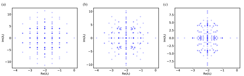
Figure S1: The Liouvillian spectrum for the dissipative XYZ model in 1D, obtained by ED. The model parameters are chosen as $N=4$, $\gamma=1$, $J_{x}=4$, and $J_{z}=2$. (a) $J_{y}=4$. The XXZ case with multiple orthogonal first decay modes. (b) $J_{y}=3$. The gapped XYZ case with multiple non-orthogonal first decay modes. (c) $J_{y}=0.5$. The “gapless” XYZ case with only one first decay mode. The color shade stands for the degeneracy of each eigenvalue $\lambda_{i}$.

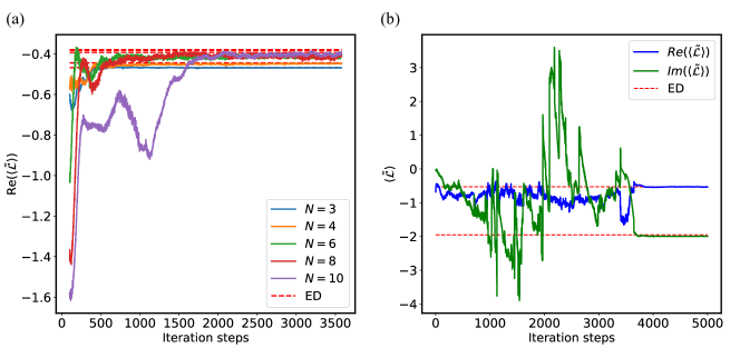
Figure S2: The convergence for the Liouvillian gap of the 1D dissipative XYZ model, obtained by the RBM approach. (a) $\text{Re}\langle\tilde{\mathcal{L}}\rangle$ as a function of the iteration steps for different lattice size $N$. $J_{x}=4$, $J_{y}=0.5$, $J_{z}=2$, and $\gamma=1$. The systems lie in the “gapless” XYZ phase with only one first decay mode. (b) $\text{Re}\langle\tilde{\mathcal{L}}\rangle$ and $\text{Im}\langle\tilde{\mathcal{L}}\rangle$ as a function of the iteration steps for the gapped XYZ phase. $N=4$, $J_{x}=4$, $J_{y}=3$, $J_{z}=2$ and $\gamma=1$. There exist multiple non-orthogonal first decay modes so that we need the joint evolution $\mathcal{L}+i\beta\mathcal{L}$ mentioned in the first section. The ancillary $\rho^{\prime}_{0}$ used here corresponds to the bi-base state with all spins pointing down.

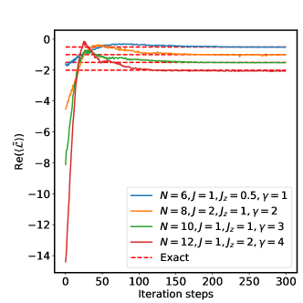
Figure S3: The convergence of the Liouvillian gap for the 1D dissipative long-range XXZ model (See Eqn. S49), obtained by the RBM approach. Different lines correspond to different lattice size $N$ and model parameters $J,J_{z},\gamma$. $\alpha=1$. The ancillary $\rho^{\prime}_{0}$ used here corresponds to the bi-base state with all spins pointing down.

References

- Breuer and Petruccione (2007) H.-P. Breuer and F. Petruccione, The theory of open quantum systems (Oxford University Press, Oxford, 2007).
- Lidar (2019) D. A. Lidar, “Lecture notes on the theory of open quantum systems,” arXiv:1902.00967 (2019).
- Noh and Angelakis (2016) C. Noh and D. G. Angelakis, “Quantum simulations and many-body physics with light,” Rep. Prog. in Phys. 80, 016401 (2016).
- Nielsen and Chuang (2010) M. A. Nielsen and I. L. Chuang, Quantum computation and quantum information (Cambridge university press, 2010).
- Medvedyeva et al. (2016) M. V. Medvedyeva, F. H. L. Essler, and T. c. v. Prosen, “Exact bethe ansatz spectrum of a tight-binding chain with dephasing noise,” Phys. Rev. Lett. 117, 137202 (2016).
- Prosen (2008) T. Prosen, “Third quantization: a general method to solve master equations for quadratic open fermi systems,” New Journal of Physics 10, 043026 (2008).
- Banchi et al. (2017) L. Banchi, D. Burgarth, and M. J. Kastoryano, “Driven quantum dynamics: Will it blend?” Phys. Rev. X 7, 041015 (2017).
- Rowlands and Lamacraft (2018) D. A. Rowlands and A. Lamacraft, “Noisy spins and the richardson-gaudin model,” Phys. Rev. Lett. 120, 090401 (2018).
- Ribeiro and Prosen (2019) P. Ribeiro and T. c. v. Prosen, “Integrable quantum dynamics of open collective spin models,” Phys. Rev. Lett. 122, 010401 (2019).
- Shibata and Katsura (2019a) N. Shibata and H. Katsura, “Dissipative spin chain as a non-hermitian kitaev ladder,” Phys. Rev. B 99, 174303 (2019a).
- Shibata and Katsura (2019b) N. Shibata and H. Katsura, “Dissipative quantum ising chain as a non-hermitian ashkin-teller model,” Phys. Rev. B 99, 224432 (2019b).
- Sá et al. (2020) L. Sá, P. Ribeiro, and T. Prosen, “Spectral and steady-state properties of random liouvillians,” Journal of Physics A: Mathematical and Theoretical (2020).
- Ziolkowska and Essler (2020) A. A. Ziolkowska and F. H. Essler, “Yang-baxter integrable lindblad equations,” SciPost Physics 8, 044 (2020).
- Nakagawa et al. (2020) M. Nakagawa, N. Kawakami, and M. Ueda, “Exact liouvillian spectrum of a one-dimensional dissipative hubbard model,” arXiv:2003.14202 (2020).
- Buča et al. (2020) B. Buča, C. Booker, M. Medenjak, and D. Jaksch, “Bethe ansatz approach for dissipation: exact solutions of quantum many-body dynamics under loss,” New Journal of Physics 22, 123040 (2020).
- Lloyd (1993) S. Lloyd, “Quantum-mechanical computers and uncomputability,” Phys. Rev. Lett. 71, 943 (1993).
- Cubitt et al. (2015) T. S. Cubitt, D. Perez-Garcia, and M. M. Wolf, “Undecidability of the spectral gap,” Nature 528, 207 (2015).
- Bausch et al. (2020) J. Bausch, T. S. Cubitt, A. Lucia, and D. Perez-Garcia, “Undecidability of the spectral gap in one dimension,” Phys. Rev. X 10, 031038 (2020).
- Weimer et al. (2019) H. Weimer, A. Kshetrimayum, and R. Orús, “Simulation methods for open quantum many-body systems,” arXiv:1907.07079 (2019).
- Verstraete et al. (2004) F. Verstraete, J. J. García-Ripoll, and J. I. Cirac, “Matrix product density operators: Simulation of finite-temperature and dissipative systems,” Phys. Rev. Lett. 93, 207204 (2004).
- Zwolak and Vidal (2004) M. Zwolak and G. Vidal, “Mixed-state dynamics in one-dimensional quantum lattice systems: A time-dependent superoperator renormalization algorithm,” Phys. Rev. Lett. 93, 207205 (2004).
- Cai and Barthel (2013) Z. Cai and T. Barthel, “Algebraic versus exponential decoherence in dissipative many-particle systems,” Phys. Rev. Lett. 111, 150403 (2013).
- Mascarenhas et al. (2015) E. Mascarenhas, H. Flayac, and V. Savona, “Matrix-product-operator approach to the nonequilibrium steady state of driven-dissipative quantum arrays,” Phys. Rev. A 92, 022116 (2015).
- Cui et al. (2015) J. Cui, J. I. Cirac, and M. C. Bañuls, “Variational matrix product operators for the steady state of dissipative quantum systems,” Phys. Rev. Lett. 114, 220601 (2015).
- Žnidarič (2015) M. Žnidarič, “Relaxation times of dissipative many-body quantum systems,” Phys. Rev. E 92, 042143 (2015).
- Werner et al. (2016) A. H. Werner, D. Jaschke, P. Silvi, M. Kliesch, T. Calarco, J. Eisert, and S. Montangero, “Positive tensor network approach for simulating open quantum many-body systems,” Phys. Rev. Lett. 116, 237201 (2016).
- Gangat et al. (2017) A. A. Gangat, T. I, and Y.-J. Kao, “Steady states of infinite-size dissipative quantum chains via imaginary time evolution,” Phys. Rev. Lett. 119, 010501 (2017).
- Kshetrimayum et al. (2017) A. Kshetrimayum, H. Weimer, and R. Orús, “A simple tensor network algorithm for two-dimensional steady states,” Nat. Commun. 8, 1 (2017).
- Finazzi et al. (2015) S. Finazzi, A. Le Boité, F. Storme, A. Baksic, and C. Ciuti, “Corner-space renormalization method for driven-dissipative two-dimensional correlated systems,” Phys. Rev. Lett. 115, 080604 (2015).
- Rota et al. (2019) R. Rota, F. Minganti, C. Ciuti, and V. Savona, “Quantum critical regime in a quadratically driven nonlinear photonic lattice,” Phys. Rev. Lett. 122, 110405 (2019).
- Jin et al. (2016) J. Jin, A. Biella, O. Viyuela, L. Mazza, J. Keeling, R. Fazio, and D. Rossini, “Cluster mean-field approach to the steady-state phase diagram of dissipative spin systems,” Phys. Rev. X 6, 031011 (2016).
- Nagy and Savona (2018) A. Nagy and V. Savona, “Driven-dissipative quantum monte carlo method for open quantum systems,” Phys. Rev. A 97, 052129 (2018).
- Yan et al. (2018) Z. Yan, L. Pollet, J. Lou, X. Wang, Y. Chen, and Z. Cai, “Interacting lattice systems with quantum dissipation: A quantum monte carlo study,” Phys. Rev. B 97, 035148 (2018).
- Casteels et al. (2018) W. Casteels, R. M. Wilson, and M. Wouters, “Gutzwiller monte carlo approach for a critical dissipative spin model,” Phys. Rev. A 97, 062107 (2018).
- Goodfellow et al. (2016) I. Goodfellow, Y. Bengio, and A. Courville, Deep learning (MIT press, 2016).
- Hartmann and Carleo (2019) M. J. Hartmann and G. Carleo, “Neural-network approach to dissipative quantum many-body dynamics,” Phys. Rev. Lett. 122, 250502 (2019).
- Vicentini et al. (2019) F. Vicentini, A. Biella, N. Regnault, and C. Ciuti, “Variational neural-network ansatz for steady states in open quantum systems,” Phys. Rev. Lett. 122, 250503 (2019).
- Nagy and Savona (2019) A. Nagy and V. Savona, “Variational quantum monte carlo method with a neural-network ansatz for open quantum systems,” Phys. Rev. Lett. 122, 250501 (2019).
- Yoshioka and Hamazaki (2019) N. Yoshioka and R. Hamazaki, “Constructing neural stationary states for open quantum many-body systems,” Phys. Rev. B 99, 214306 (2019).
- Carleo and Troyer (2017) G. Carleo and M. Troyer, “Solving the quantum many-body problem with artificial neural networks,” Science 355, 602 (2017).
- Torlai and Melko (2018) G. Torlai and R. G. Melko, “Latent space purification via neural density operators,” Phys. Rev. Lett. 120, 240503 (2018).
- Carrasquilla et al. (2019) J. Carrasquilla, G. Torlai, R. G. Melko, and L. Aolita, “Reconstructing quantum states with generative models,” Nature Machine Intelligence 1, 155 (2019).
- Banchi et al. (2018) L. Banchi, E. Grant, A. Rocchetto, and S. Severini, “Modelling non-markovian quantum processes with recurrent neural networks,” New Journal of Physics 20, 123030 (2018).
- Cai and Liu (2018) Z. Cai and J. Liu, “Approximating quantum many-body wave functions using artificial neural networks,” Phys. Rev. B 97, 035116 (2018).
- Schmitt and Heyl (2020) M. Schmitt and M. Heyl, “Quantum many-body dynamics in two dimensions with artificial neural networks,” Phys. Rev. Lett. 125, 100503 (2020).
- Sorella et al. (2007) S. Sorella, M. Casula, and D. Rocca, “Weak binding between two aromatic rings: Feeling the van der waals attraction by quantum monte carlo methods,” J. Chem. Phys. 127, 014105 (2007).
- Deng et al. (2017) D.-L. Deng, X. Li, and S. Das Sarma, “Quantum entanglement in neural network states,” Phys. Rev. X 7, 021021 (2017).
- Rossatto and Villas-Boas (2016) D. Z. Rossatto and C. J. Villas-Boas, “Relaxation time for monitoring the quantumness of an intense cavity field,” Phys. Rev. A 94, 033819 (2016).
- Kessler et al. (2012) E. M. Kessler, G. Giedke, A. Imamoglu, S. F. Yelin, M. D. Lukin, and J. I. Cirac, “Dissipative phase transition in a central spin system,” Phys. Rev. A 86, 012116 (2012).
- Minganti et al. (2018) F. Minganti, A. Biella, N. Bartolo, and C. Ciuti, “Spectral theory of liouvillians for dissipative phase transitions,” Phys. Rev. A 98, 042118 (2018).
- Song et al. (2019) F. Song, S. Yao, and Z. Wang, “Non-hermitian skin effect and chiral damping in open quantum systems,” Phys. Rev. Lett. 123, 170401 (2019).
- (52) See Supplemental Material at [URL will be inserted by publisher] for details on the stochastic reconfiguration, computational cost, analytical solution of the full Liouvillian spectrum for the dissipative XXZ model, and more numerical data, which includes Refs. Metropolis et al. (1953); Melko et al. (2019); Yupeng Wang and Shi (2015); Lee et al. (2013b); Huybrechts et al. (2020).
- Vieijra et al. (2020) T. Vieijra, C. Casert, J. Nys, W. De Neve, J. Haegeman, J. Ryckebusch, and F. Verstraete, “Restricted boltzmann machines for quantum states with non-abelian or anyonic symmetries,” Phys. Rev. Lett. 124, 097201 (2020).
- Choo et al. (2018) K. Choo, G. Carleo, N. Regnault, and T. Neupert, “Symmetries and many-body excitations with neural-network quantum states,” Phys. Rev. Lett. 121, 167204 (2018).
- Lee et al. (2013a) T. E. Lee, S. Gopalakrishnan, and M. D. Lukin, “Unconventional magnetism via optical pumping of interacting spin systems,” Phys. Rev. Lett. 110, 257204 (2013a).
- Rota et al. (2017) R. Rota, F. Storme, N. Bartolo, R. Fazio, and C. Ciuti, “Critical behavior of dissipative two-dimensional spin lattices,” Phys. Rev. B 95, 134431 (2017).
- Rota et al. (2018) R. Rota, F. Minganti, A. Biella, and C. Ciuti, “Dynamical properties of dissipative xyz heisenberg lattices,” New Journal of Physics 20, 045003 (2018).
- Huybrechts and Wouters (2019) D. Huybrechts and M. Wouters, “Cluster methods for the description of a driven-dissipative spin model,” Phys. Rev. A 99, 043841 (2019).
- Torres (2014) J. M. Torres, “Closed-form solution of lindblad master equations without gain,” Phys. Rev. A 89, 052133 (2014).
- Saito (2017) H. Saito, “Solving the bose–hubbard model with machine learning,” J. Phys. Soc. Jpn. 86, 093001 (2017).
- Nomura et al. (2017) Y. Nomura, A. S. Darmawan, Y. Yamaji, and M. Imada, “Restricted boltzmann machine learning for solving strongly correlated quantum systems,” Phys. Rev. B 96, 205152 (2017).
- Choo et al. (2020) K. Choo, A. Mezzacapo, and G. Carleo, “Fermionic neural-network states for ab-initio electronic structure,” Nat. Commun. 11, 1 (2020).
- Arora and Barak (2009) S. Arora and B. Barak, Computational complexity: a modern approach (Cambridge University Press, 2009).
- Schollwöck (2005) U. Schollwöck, “The density-matrix renormalization group,” Rev. Mod. Phys. 77, 259 (2005).
- Gao and Duan (2017) X. Gao and L.-M. Duan, “Efficient representation of quantum many-body states with deep neural networks,” Nat. Commun. 8, 1 (2017).
- Liu et al. (2020) Z. Liu, L. M. Duan, and D.-L. Deng, “Solving quantum master equations with deep quantum neural networks,” arXiv:2008.05488 (2020).
- Preskill (2018) J. Preskill, “Quantum computing in the NISQ era and beyond,” Quantum 2, 79 (2018).
- Metropolis et al. (1953) N. Metropolis, A. W. Rosenbluth, M. N. Rosenbluth, A. H. Teller, and E. Teller, “Equation of state calculations by fast computing machines,” J. Chem. Phys. 21, 1087 (1953).
- Melko et al. (2019) R. G. Melko, G. Carleo, J. Carrasquilla, and J. I. Cirac, “Restricted boltzmann machines in quantum physics,” Nat. Phys. 15, 887 (2019).
- Yupeng Wang and Shi (2015) J. C. Yupeng Wang, Wen-Li Yang and K. Shi, Off-Diagonal Bethe Ansatz for Exactly Solvable Models (Springer, Berlin, Heidelberg, 2015).
- Lee et al. (2013b) T. E. Lee, S. Gopalakrishnan, and M. D. Lukin, “Unconventional magnetism via optical pumping of interacting spin systems,” Phys. Rev. Lett. 110, 257204 (2013b).
- Huybrechts et al. (2020) D. Huybrechts, F. Minganti, F. Nori, M. Wouters, and N. Shammah, “Validity of mean-field theory in a dissipative critical system: Liouvillian gap, -symmetric antigap, and permutational symmetry in the model,” Phys. Rev. B 101, 214302 (2020).