Uncertain Spatial Data Management:
An Overview

Abstract

Both the current trends in technology such as smart phones, general mobile devices, stationary sensors, and satellites as we as a new user mentality of using this technology to voluntarily share enriched location information produces a flood of geo-spatial and geo-spatio-temporal data. This data flood provides a tremendous potential of discovering new and useful knowledge. But in addition to the fact that measurements are imprecise, spatial data is often interpolated between discrete observations. To reduce communication and bandwidth utilization, data is often subjected to a reduction, thereby eliminating some of the known/recorded values. These issues introduce the notion of uncertainty in the context of spatio-temporal data management, an aspect raising imminent need for scalable and flexible solutions. The main scope of this chapter is to survey existing techniques for managing, querying, and mining uncertain spatio-temporal data. First, this chapter surveys common data representations for uncertain data, explains the commonly used possible worlds semantics to interpret an uncertain database, and surveys existing system to process uncertain data. Then this chapter defines the notion of different probabilistic result semantics to distinguish the task of enrich individual objects with probabilities rather than enriched entire results with probabilities. To distinguish between result semantics is important, as for many queries, the problem of computing object-level result probabilities can be done efficiently, whereas the problem of computing probabilities of entire results is often exponentially hard. Then, this chapter provides an overview over probabilistic query predicates to quantify the required probability of a result to be included in the result. Finally, this chapter introduces a novel paradigm to efficiently answer any kind of query on uncertain data: the Paradigm of Equivalent Worlds, which groups the exponential set of possible database worlds into a polynomial number of set of equivalent worlds that can be processed efficiently. Examples and use-cases of querying uncertain spatial data are provided using the example of uncertain range queries.

1 Introduction

Due to the proliferation of handheld GPS enabled devices, spatial and spatio-temporal data is generated, stored, and published by billions of users in a plethora of applications. By mining this data, and thus turning it into actionable information, The McKinsey Global Institute projects a “$600 billion potential annual consumer surplus from using personal location data globally”.

As the volume, variety and velocity of spatial data has increased sharply over the last decades, uncertainty has increased as well. Until the early 21st century, spatial data available for geographic information science (GIS) was mainly collected, curated, standardized [50, 49], and published by authoritative sources such as the United States Geological Survey (USGS) [101]. Now, data used for spatial data mining is often obtained from sources of volunteered geographic information (VGI) [98, 84]. Consequentially, our ability to unearth valuable knowledge from large sets of such spatial data is often impaired by the uncertainty of the data which geography has been named the “the Achilles heel of GIS” [53] for many reasons:

• Imprecision is caused by physical limitations of sensing devices and connection errors, for instance in geographic information system using cell-phone GPS [38],

• Data records may be obsolete. In geo-social networks and microblogging platforms such as Twitter, users may update their location infrequently, yielding uncertain location information in-between data records [63],

• Data can be obtained from unreliable sources, such as volunteered geographic information like data in Open-Street-Map [84], where data is obtained from individual users, which may incur inaccurate or plain wrong data, deliberately or due to human error [54],

• Data sets pertaining to specific questions may be too small to answer questions reliably. Proper statistical inference is required to draw significant conclusions from the data and to avoid basing decisions upon spurious mining results [56, 24].

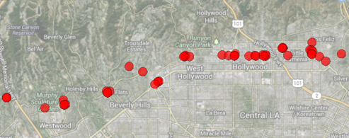
Figure 1: User locations in a Location-based social network (Gowalla) over a day.

To illustrate uncertainty in spatial and spatio-temporal data, Figure 1 shows a typical one-day “trajectory” of a prolific user in the location-based social network Gowalla (data taken from [35]). While a trajectory is usually defined as a function that continuously maps time to locations, we see that in this case, we can only observe the user at discrete times, having hours in-between subsequent location updates. Where was the user located in-between these updates? Should we use dead reckoning techniques to interpolate the locations or should be assume that the user stays at a location until next update? Also, users may spoof their location [116], either to protect their privacy or to gain advantages within the location-based social network. Given this uncertainty, how certain can we be about the location of the user at a given time $t$? And how does the uncertainty increase as location updates become more sparse and obsolete? The goal of this chapter is to provide a comprehensive overview of models and techniques to deal with uncertainty. To handle uncertainty, we must first remind ourselves that a database models an aspect of the real world, the universe of discourse. Information observed and stored in a database may deviate from the real-world. For reliable decision making, we need to quantify the uncertainty of attribute values stored in the database and consider potentially missing objects that may change mining results.

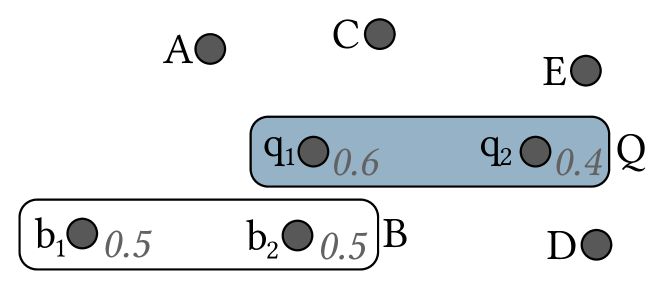
Figure 2: Exemplary Uncertain Database.

Example 1

As a running example used through this chapter, consider Figure 2 which shows a toy uncertain spatial database. In this example, two objects, $Q$ and $B$ have uncertain locations, indicated by alternative locations $\{q_{1},q_{2}\}$ of $Q$ and alternative locations $\{b_{1},b_{2}\}$ of $B$. In this book chapter, we will survey methods to answer questions such as “What object is closest to Q?”, or “What is the probability of $B$ to be one of the two-nearest neighbors of $Q$?”

To answer such queries, we first need a crisp definition of what it means for an uncertain object to be a (probabilistic) nearest neighbor of a query object and how the probability of such an event is defined. This chapter gives a widely used interpretation of uncertain databases using Possible Worlds Semantics. This interpretation allows to answer arbitrary queries on uncertain data, but at a computational cost exponential in the number of uncertain objects. For efficient processing, this chapter defines a paradigm of querying uncertain data that allows to efficiently answer many spatial queries on uncertain spatial data.

managing and querying uncertain spatial data. Parts of this section have been presented in the form of presentation slides at recent conference tutorials at VLDB 2010 ([90]), ICDE 2014 ([31]), ICDE 2017 ([122]), and MDM 2020 [121]. This chapter is subdivided to give a survey of definitions, notions and techniques used in the field of querying and mining uncertain spatio-temporal data.

• Section 2 presents a survey of state-of-the-art data representations models used in the field of uncertain data management. This section explain discrete and continuous models for uncertain objects.

• To interpret queries on a database of uncertain objects, well-defined semantics of uncertain database are required. For this purpose, Section 3 introduces the possible world semantics for uncertain data.

• To run queries on uncertain spatial data, existing systems for uncertain spatial database management are surveyed in Section 4.

• Given an uncertain database, the result of a probabilistic query can be interpreted in two ways as elaborated in Section 5. This distinction between different probabilistic result semantics is not made explicitly in any related work, but is required to gain a deep understanding of problems in the field of querying uncertain spatial data and their complexity.

• Section 6 gives an overview over probabilistic query predicates. A probabilistic query predicate defines the requirements for the probability of a candidate result to be returned as a query result.

• Section 7 introduces a novel paradigm for uncertain data to efficiently answer any kind of query using possible world semantics. This Paradigm of Equivalent Worlds generalizes existing solutions by identifying requirements a query must satisfy in order to have a polynomial solution.

• Section 8 presents efficient solutions for the problem of computing range queries on uncertain spatial databases. For this purpose, the paradigm of equivalent worlds is leveraged to compute the distribution of the sum of a Poisson-binomial distributed random variable, a problem that is paramount for many spatial queries on uncertain data.

• Section 9 gives an overview of specific research problems using uncertain spatial and spatio-temporal data, and surveys state-of-the-art solutions.

• Finally, Section 10 concludes this book chapter and sketches future research directions that can be opened by leveraging the Paradigm of Equivalent Worlds to new applications and query types.

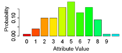
(a) Discrete Probability Mass Function

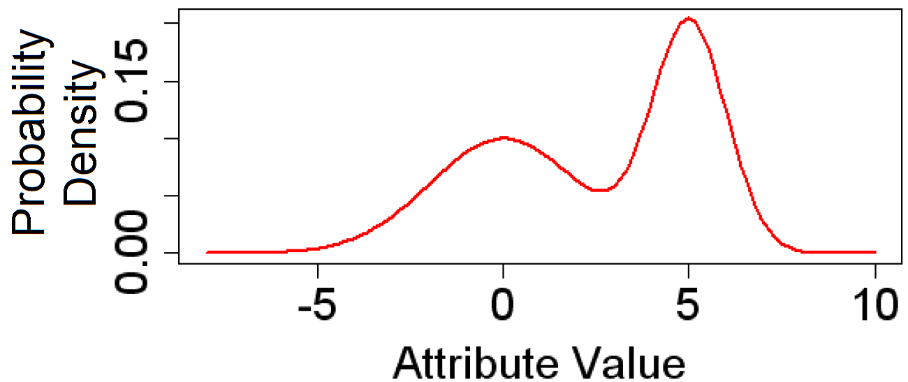
(b) Continuous Prob. Density Function

Figure 3: Models for Uncertain Attributes

2 Discrete and Continuous Models for Uncertain Data

An object is uncertain if at least one attribute of $o$ is uncertain. The uncertainty of an attribute can be captured in a discrete or continuous way. A discrete model uses a probability mass function (pmf) to describe the location of an uncertain object. In essence, such a model describes an uncertain object by a finite number of alternative instances, each with an associated probability [61, 86], as shown in Figure 3(a). In contrast, a continuous model uses a continuous probability density function (pdf), like Gaussian, uniform, Zipfian, or a mixture model, as depicted in Figure 3(b), to represent object locations over the space. Thus, in a continuous model, the number of possible attribute values is uncountably infinite. In order to estimate the probability that an uncertain attribute value is within an interval, integration of its pdf over this interval is required [99]. The random variables corresponding to each uncertain attribute of an object $o$ can be arbitrarily correlated.

To capture positional uncertainty, such models can be applied by treating longitude and latitude (and optionally elevation) as two (three) uncertain attributes. In the case of discrete positional uncertainty, the position of an object $A$ is given by a discrete set $a_{1},...,a_{m}$ of $m\in\mathbb{N}$ possible alternatives in space, as exemplarily depicted in Figure 4(a) for two uncertain objects $A$ and $B$. Each alternative $a_{i}$ is associated with a probability value $p(a_{i})$, which may for example be derived from empirical information about the turn probabilities of intersection in an underlying road network. In a nutshell, the position $A$ is a random variable, defined by a probability mass function $\mbox{pdf}_{A}$ that maps each alternative position $a_{i}$ to its corresponding probability $p(a_{i})$, and that maps all other positions in space to a zero probability. An important property of uncertain spatial databases is the inherent correlation of spatial attributes. In the example shown in Figure 4(a) it can be observed that the uncertain attributes $a$ and $b$ are highly correlated: given the value of one attribute, the other attribute is certain, as there is no two alternatives of objects $A$ and $B$ having identical attribute values in either attribute.

Clearly, it must hold that the sum of probabilities of all alternatives must sum to at most one:

$$\sum_{i=1}^{m}p(a_{i})\leq 1$$

In the case where $\sum_{i=1}^{m}p(a_{i})\leq 1$ object $A$ has a non-zero probability of $1-\sum_{i=1}^{m}p(a_{i})\geq 0$ to not exist at all. This case is called existential uncertainty, and $A$ is denoted as existentially uncertain [112]. If the total number of possible instances $m$ is greater than one, $A$ is denoted as attribute uncertain. In the context of uncertain spatial data, attribute uncertainty is also referred to as positional uncertainty or location uncertainty. An object can be both existentially uncertain and attribute uncertain. In Figure 4(a), object $A$ is both existentially uncertain and attribute uncertain, while object $B$ is attribute uncertain but does exist for certain.

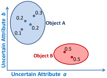
(a) Discrete Case

(b) Continuous Case

Figure 4: Uncertain Objects

In the case of continuous uncertainty, the number of possible alternative positions of an object $A$ is infinite, and given by the non-zero domain of the probability density function $\mbox{pdf}_{x}$. The probability of $A$ to occur in some spatial region $r$ is given by integration

$$\int_{r}pdf_{A}(x)dx.$$

Since arbitrary pdfs may be represented by an uncountably infinite large number of ($position$, $probability$) pairs, such pdfs may require infinite space to represent. For this reason, assumptions on the shape of a pdf are made in practice. All continuous models for positionally uncertain data therefore use parametric pdfs, such as Gaussian, uniform, Zipfian, mixture models, or parametric spline representations. For illustration purpose, Figure 4(b) depicts three uncertain objects modelled by a mixture of gaussian pdfs. Similar to the discrete case, the constraint

$$\int_{\mathbb{R}^{d}}pdf_{A}(x)dx\leq 1$$

must be satisfied, where $\mathbb{R}^{d}$ is a $d$ dimensional vector space. In the case of spatial data, $d$ usually equals two or three. The notion of existentially and attribute uncertain objects is defined analogous to the discrete case.

The following section reviews related work and state-of-the-art on the field of modeling uncertain data.

2.1 Existing Models for Uncertain Data

This section gives a brief survey on existing models for uncertain spatial data used in the database community. Many of the presented models have been developed to model uncertainty in relational data, but can be easily adapted to model uncertain spatial data. Since one of the main challenges of modeling uncertain data is to capture correlation between uncertain objects, this section will elaborate details on how state-of-the-art approaches tackles this challenge. Both discrete and continuous models are presented.

Discrete Models

In addition to reviewing related work defining discrete uncertainty models, the aim of this section is to put these papers into context of Section 2. In particular, models which are special cases or equivalent to the model presented in Section 2 will be identified, and proper mappings to Section 2 will be given.

Independent Tuple Model. Initial models have been proposed simultaneously and independently in [52, 118]. These works assume a relational model in which each tuple is associated with a probability describing its existential uncertainty. All tuples are considered independent from each other. This simple model can be seen as a special case of the model presented in Section 2, where only existential uncertain but no attribute uncertainty is modelled.

Block-Independent Disjoint Tuples Model and X-Tuple model A more recent and the currently most prominent approach to model discrete uncertainty is the block-independent disjoint tuples model ([41]), which can capture mutual exclusion between tuples in uncertain relational databases. A probabilistic database is called block independent-disjoint if the set of all possible tuples can be partitioned into blocks such that tuples from the same block are disjoint events, and tuples from distinct blocks are independent. A commonly used example of a block-independent disjoint tuples model is the Uncertainty-Lineage Database Model([13, 91, 97, 110, 111]), also called X-Relation Model or simply X-Tuple Model that has been developed for relational data. In this model, a probabilistic database is a finite set of probabilistic tables. A probabilistic table $T$ contains a set of (uncertain) tuples, where each tuple $t\in T$ is associated with a membership probability value $Pr(t)>0$. A generation rule $R$ on a table $T$ specifies a set of mutually exclusive tuples in the form of $R:t_{r_{1}}\oplus...\oplus t_{r_{m}}$ where $t_{r_{i}}\in T(1\leq i\leq m)$ and $P(R):=\sum_{i=1}^{m}t_{r_{i}}\leq 1$. The rule R constrains that, among all tuples $t_{r_{1}},...,t_{r_{m}}$ involved in the rule, at most one tuple can appear in a possible world. The case where $P(R)<1$ the probability $1-P(R)$ corresponds to the probability that no tuple contained in rule $R$ exists. It is assumed that for any two rules $R_{1}$ and $R_{2}$ it holds that $R_{1}$ and $R_{2}$ do not share any common tuples, i.e., $R_{1}\cap R_{2}=\emptyset$. In this model, a possible world $w$ is a subset of $T$ such that for each generation rule $R$, $w$ contains exactly one tuple involved in $R$ if $P(R)=1$, or $w$ contains 0 or 1 tuple involved in $R$ if $Pr(R)<1$.

This model can be translated to a discrete model for uncertain spatial data as discussed in Section 2 by interpreting the set $T$ as the set of all possible locations of all objects, and interpreting each rule $R$ as an uncertain spatial object having alternatives $t_{r_{i}}$. The constraint that no two rules may share any common tuples translates into the assumption of mutually independent spatial objects. Finally, the case $P(R)<1$ corresponds to the case of existential uncertainty (see Section 2).

A similar block-independent disjoint tuples model is called p-or-set [89] and can be translated to the model described in Section 2 analogously. In [8], another model for uncertainty in relational databases has been proposed that allows to represent attribute values by sets of possible values instead of single deterministic values. This work extends relational algebra by an operator for computing possible results. A normalized representation of uncertain attributes, which essentially splits each uncertain attribute into a single relation, a so-called U-relation, allows to efficiently answer projection-selection-join queries. The main drawback of this model is that it is not possible to compute probabilities of the returned possible results. Sen and Deshpande [95] propose a model based on a probabilistic graphical model, for explicitly modeling correlations among tuples in a probabilistic database. Strategies for executing SQL queries over such data have been developed in this work. The main drawback of using the proposed graphical model is its complexity, which grows exponential in the number of mutually correlated tuples. This is a general drawback for graphical models such as Bayesian networks and graphical Markov models, where even a factorized representation may fail to reduce the complexity sufficiently: The idea of a factorized representation is to identify conditional independencies. For example, if a random variable $C$ depends on random variables $A$ and $B$, then the distribution of $C$ has to be given relative to all combination of realizations of $A$ and $B$. If however, $C$ is conditionally independent of $A$, i.e., $B$ depends on $A$, $C$ depends on $B$, and $C$ only transitively depends on $A$, then it is sufficient to store the distribution of $C$ relative only to the realizations of $B$. Nevertheless, if for a given graphical model a random variable depends on more than a hand-full of other random variables, then the corresponding model will become infeasible.

And/Xor Tree Model. A very recent work by Li and Deshpande [66] extends the block-independent disjoint tuples model by adding support for mutual co-existence. Two events satisfy the mutual co-existence correlation if in any possible world, either both happen or neither occurs. This work allows both mutual exclusiveness and mutual co-existence to be specified in a hierarchical manner. The resulting tree structure is called an and/xor tree. While theoretically highly relevant, the and/xor tree model becomes impracticable in large database having non-trivial object dependencies, as it grows exponentially in the number of database objects.

If not stated otherwise, this chapter will apply the block-independent disjoint tuples model as model of choice for discrete uncertain data.

Continuous Models

In general, similarity search methods based on continuous models involve expensive integrations of the PDFs, hence special approximation and indexing techniques for efficient query processing are typically employed [34, 99]. In order to increase quality of approximations, and in order to reduce the computational complexity, a number of models have been proposed making assumptions on the shape of object PDFs. Such assumptions can often be made in applications where the uncertain values follow a specific parametric distribution, e.g. a uniform distribution [32, 29] or a Gaussian distribution [29, 44, 85]. Multiple such distributions can be mixed to obtain a mixture model [100, 22]. To approximate arbitrary PDFs, [67] proposes to use polynomial spline approximations.

3 Possible World Semantics

In an uncertain spatial database $\mathcal{D}=\{U_{1},...,U_{N}\}$, the location of an object is a random variable. Consequently, if there is at least one uncertain object, the data stored in the database becomes a random variable. To interpret, that is, to define the semantics of a database that is, in itself, a random variable, the concept of possible worlds is described in this section.

Definition 1 (Possible World Semantics)

A possible world $w=\{u_{1}^{a_{1}},...,u_{N}^{a_{N}}\}$ is a set of instances containing at most one instance $u_{i}^{a_{i}}\in U_{i}$ from each object $U_{i}\in\mathcal{D}$. The set of all possible worlds is denoted as $\mathcal{W}$. The total probability of an uncertain world $P(w\in\mathcal{W})$ is derived from the chain rule of conditional probabilities:

$$P(w):=P(\bigwedge_{u_{i}^{a_{i}}\in w}U_{i}=u_{i}^{a_{i}})=\prod_{i=1}^{N}P(u_{i}^{a_{i}}|\bigwedge_{j<i}u_{j}^{a_{j}}).$$ (1)

By definition, all worlds $w$ having a zero probability $P(w)=0$ are excluded from the set of possible worlds $\mathcal{W}$. Equation 1 can be used if conditional probabilities of the position of objects given the position of other objects are known, e.g. by a given graphical model such as a Bayesian network or a Markov model. In many applications where independence between object locations can be assumed, as well as in applications where only the marginal probabilities $P(u_{i}^{a_{i}})$ are known, and thus independence has to be assumed due to lack of better knowledge of a dependency model, the above equation simplifies to

$$P(w)=\prod_{i=1}^{N}P(u_{i}^{a_{i}}).$$ (2)

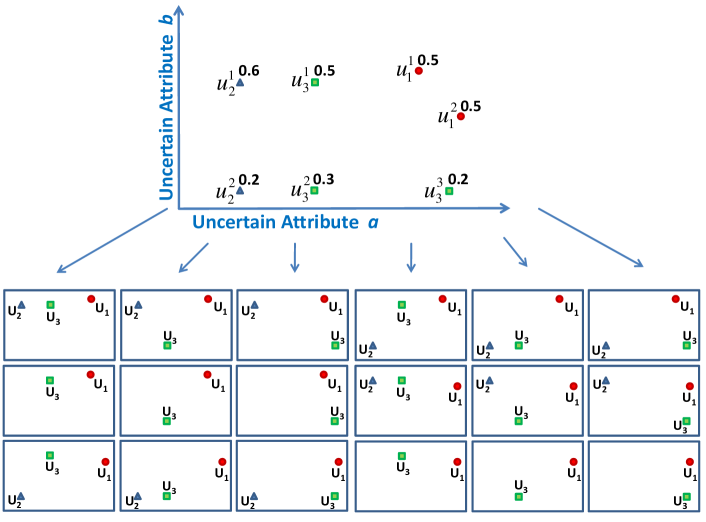
Figure 5: An uncertain database and all of its possible worlds.

Table 1: Possible worlds corresponding to Figure 5.

World	Probability	World	Probability
$\{u_{1}^{1},u_{2}^{1},u_{3}^{1}\}$	$0.5\cdot 0.7\cdot 0.5=0.175$	$\{u_{1}^{2},u_{2}^{1},u_{3}^{1}\}$	$0.5\cdot 0.7\cdot 0.5=0.175$
$\{u_{1}^{1},u_{2}^{1},u_{3}^{2}\}$	$0.5\cdot 0.7\cdot 0.3=0.105$	$\{u_{1}^{2},u_{2}^{1},u_{3}^{2}\}$	$0.5\cdot 0.7\cdot 0.3=0.105$
$\{u_{1}^{1},u_{2}^{1},u_{3}^{3}\}$	$0.5\cdot 0.7\cdot 0.2=0.07$	$\{u_{1}^{2},u_{2}^{1},u_{3}^{3}\}$	$0.5\cdot 0.7\cdot 0.2=0.07$
$\{u_{1}^{1},u_{2}^{2},u_{3}^{1}\}$	$0.5\cdot 0.2\cdot 0.5=0.05$	$\{u_{1}^{2},u_{2}^{2},u_{3}^{1}\}$	$0.5\cdot 0.2\cdot 0.5=0.05$
$\{u_{1}^{1},u_{2}^{2},u_{3}^{2}\}$	$0.5\cdot 0.2\cdot 0.3=0.03$	$\{u_{1}^{2},u_{2}^{2},u_{3}^{2}\}$	$0.5\cdot 0.2\cdot 0.3=0.03$
$\{u_{1}^{1},u_{2}^{2},u_{3}^{3}\}$	$0.5\cdot 0.2\cdot 0.2=0.02$	$\{u_{1}^{2},u_{2}^{2},u_{3}^{3}\}$	$0.5\cdot 0.2\cdot 0.2=0.02$
$\{u_{1}^{1},u_{3}^{1}\}$	$0.5\cdot 0.1\cdot 0.5=0.025$	$\{u_{1}^{2},u_{3}^{1}\}$	$0.5\cdot 0.1\cdot 0.5=0.025$
$\{u_{1}^{1}u_{3}^{2}\}$	$0.5\cdot 0.1\cdot 0.3=0.015$	$\{u_{1}^{2},u_{3}^{2}\}$	$0.5\cdot 0.1\cdot 0.3=0.015$
$\{u_{1}^{1},u_{3}^{3}\}$	$0.5\cdot 0.1\cdot 0.2=0.01$	$\{u_{1}^{2},u_{3}^{3}\}$	$0.5\cdot 0.1\cdot 0.2=0.01$

Example 2

As an example, consider Figure 5 where a database consisting of three uncertain objects $\mathcal{D}=\{U_{1},U_{2},U_{3}\}$ is depicted. Objects $U_{1}=\{u_{1}^{1},u_{1}^{2}\}$ and $U_{2}=\{u_{2}^{1},u_{2}^{2}\}$ each have two possible instances, while object $U_{3}=\{u_{3}^{1},u_{3}^{2},u_{3}^{3}\}$ has three possible instances. The probabilities of these instances is given as $P(u_{1}^{1})=P(u_{1}^{2})=0.5$, $P(u_{2}^{1})=0.7$, $P(u_{2}^{2})=0.2$, $P(u_{3}^{1})=0.5$, $P(u_{3}^{2})=0.3$, $P(u_{3}^{3})=0.2$. Note that object $U_{2}$ is the only object having existential uncertainty: With a probability of $1-0.7-0.2=0.1$ object $U_{2}$ does not exist at all. Assuming independence between spatial objects, the probability for the possible world where $U_{1}=u_{1}^{1}$, $U_{2}=u_{2}^{1}$ and $U_{3}=u_{3}^{1}$ is given by applying Equation 2 to obtain the product $0.5\cdot 0.7\cdot 0.5=0.175$. All possible worlds spanned by $\mathcal{D}$ are depicted in Figure 5. The probability of each possible world is shown in Table 1, including possible worlds where $U_{2}$ does not exist.

Recall that a predicate can evaluate to either true or false on a crisp (non-uncertain) database. An exemplary predicate is There are at least five database objects in a 500meter range of the location “Theresienwiese, Munich”. To evaluate a predicate $\phi$ on an uncertain database using possible world semantics, the query predicate is evaluated on each possible world. The probability that the query predicate evaluates to true is defined as the sum of probabilities of all worlds where $\phi$ is satisfied, formally:

Definition 2

Let $\mathcal{D}$ be an uncertain spatial database inducing the set of possible worlds $\mathcal{W}$, let $\phi$ be some query predicate, and let

$$\mathcal{I}(\phi,w\in\mathcal{W}):=P(\phi(\mathcal{D})|\mathcal{D}=w)\in\{0,1\}$$

be the indicator function that returns one if world $w$ satisfies $\phi$ and zero otherwise. The marginal probability $P(\phi(\mathcal{D}))$ of the event $\phi(\mathcal{D})$ that predicate $\phi$ holds in $\mathcal{D}$ is defined as follows using the theorem of total probability [123]:

$$P(\phi(\mathcal{D}))=\sum_{w\in\mathcal{W}}\mathcal{I}(\phi,w)\cdot P(w)\vspace{-0.1cm}$$ (3)

The main challenge of analyzing uncertain data is to efficiently and effectively deal with the large number of possible worlds induced by an uncertain database $\mathcal{D}$. In the case of continuous uncertain data, the number of possible worlds is uncountably infinite and expensive integration operations or numerical approximation are required for most spatial database queries and spatial data mining tasks. Even in the case of discrete uncertainty, the number of possible worlds grows exponentially in the number of objects: in the worst case, any combination of alternatives of objects may have a non-zero probability, as shown exemplary in Figure 5. This large number of possible worlds makes efficient query processing and data mining an extremely challenging problem. In particular, any problem that requires an enumeration of all possible worlds is #P-hard. In particular, a number of probabilistic problems have been proven to be in #P [102]. Following this argumentation, general query processing in the case of discrete data using object independence has proven to be a #P-hard problem [42] in the context of relational data. The spatial case is a specialization of the relation case, but clearly, the spatial case is in #P as well, which becomes evident by construction of a query having an exponentially large result, such as the query that returns all possible worlds. Consequently, there can be no universal solution that allows to answer any query in polynomial time. This implies that querying processing on models that are generalizations of the discrete case with object independence, e.g., models using continuous distribution, or models that relax the object independence assumption, must also be a #P hard problem. The result of [42] implies that there exists query predicates, for which no polynomial time solution can be given. Yet, this result does not outrule the existence of query predicates that can be answered efficiently. For example the (trivial) query that always returns the empty set of objects can be efficiently answered on uncertain spatial databases.

4 Existing Uncertain Spatial Database Management Systems

Recently developed systems provide support for spatio-temporal data in big data systems [7, 6, 79, 105, 113]. Such systems exhibit high scalability for batch-processing jobs [10, 43], but do not provide efficient solutions to handle uncertain data and to assess the reliability of results. The vivid field of managing, querying, and mining uncertain data has received tremendous attention from the database, data mining, and spatial data science communities. Recent books [3] and survey papers [4, 108, 72] provide an overview of the flurry of research papers that have appeared in these fields.

been well-studied by the database research community in the past. While the traditional database literature [25, 12, 11, 64, 51] has studied the problem of managing uncertain data, this research field has seen a recent revival, due to modern techniques for collecting inherently uncertain data. Most prominent concepts for probabilistic data management are MayBMS [9], MystiQ [23], Trio [5], and BayesStore [104]. These uncertain database management systems (UDBMS) provide solutions to cope with uncertain relational data, allowing to efficiently answer traditional queries that select subsets of data based on predicates or join different datasets based on conditions. Extensions to the UDBMS also allow answering of important classes of spatial queries such as top-k and distance-ranking queries [57, 36, 69, 18, 68]. While these existing UDBMS provide probabilistic guarantees for their query results, they offer no support for data mining tasks. A likely reason for this gap is the theoretic result of [40] which shows that the problem of answering complex queries is #P-hard in the number of database objects. To illustrate this theoretic result, imagine running a simple range query with an arbitrary query point on a database having $N$ objects each having an arbitrary non-zero probability of being in that range. Further, assume stochastic independence between these objects. In that case, any of the $2^{N}$ combinations of result objects becomes a possible result and must be returned.

Nevertheless, a number of polynomial time solutions have been proposed in the literature for various spatial query types such as nearest neighbor queries [33, 61, 58, 29], k-nearest neighbor queries [21, 78, 70, 30] and (similarity-) ranking queries [19, 37, 70, 96]. On first glance, these findings may look contradicting (unless $P=NP$), providing polynomial-time solution to a #P-hard problem. On closer look, it shows that different related work use different semantics to interpret a result. Aforementioned related works that provide polynomial time solutions for spatial queries on uncertain data make a simplifying assumption: Rather than computing the probability for each possible result, they compute the probability of each object to be part of the result. This reduces the number of probabilities that have to be reported, in the worst-case, from a number exponential in the number of database objects, to a linear number. Re-using the example of a range query on an uncertain database, it is possible to compute the probability that a single object is within the query range independent from all other objects.

Unfortunately, this simplification also yields a loss of information, as it is not possible to infer the probability of query results given only probabilities of individual objects. Let us revisit the running example from introduction, which is duplicate in Figure 6 for convenience. This example will illustrate how such an object-based approach, which computes object-individual probabilities, rather than the probabilities of result sets, may yield misleading results.

Figure 6: The Exemplary Uncertain Database from Figure 2

Example 3

Assume that the task is to simply find the probabilistic two nearest neighbors (2NN) of uncertain object $Q$. Objects $Q$ and $B$ have two alternative positions each, yielding a total of four possible worlds. For example, in one possible world, where $Q$ has location $q_{1}$ and $B$ has location $b_{1}$, the two nearest neighbors of $Q$ are $A$ and $C$. This possible world has a probability of $0.6\cdot 0.5=0.3$, obtained by assuming stochastic independence between objects. Following object-based result semantics, we can obtain probabilities of $0.3$, $0.3$, $0.6$, $0.4$, $0.4$ for objects $A$, $B$, $C$, $D$, and $E$ to be the $2$NNs of $Q$, respectively. However, this result hides any dependence between these result objects, such as objects $A$ and $B$ are mutually exclusive, while $D$ and $E$ are mutually inclusive.

Towards approximate solutions, the Monte-Carlo DB (MCDB) system [59] has been proposed, which samples possible worlds from the database, executes the query predicate on each sampled world. MCDB estimates the probability of each object to be part of the result set. However, this approach of assigning a result probability to each object, as illustrate in the example above, cannot be extended to assess the probability of result sets. The problem is that the number of possible result sets may be exponentially large. To aggregate possible worlds into groups of mutually similar worlds (having similar results), an approach has been proposed for clustering of uncertain data [120, 94] and more recently for general query processing on spatial data [92]. Revisiting the example of Figure 2, this approach reports the results of a probabilistic query 2NN query as $\{A,C\}$, $\{B,C\}$, $\{D,E\}$, having respective probabilities of $0.3$, $0.3$, and $0.4$. However, this approach ([92]) can only be applied to spatial queries that return result sets, thus cannot be applied to more complex spatial queries or data mining tasks. To further elaborate the difference between solutions that compute the probability of each object to be part of the result, and solutions that compute the probability of each result, the following section will further survey the two different “Probabilistic Result Semantics”: Object-based and Result-based.

5 Probabilistic Result Semantics

Recall that a spatial similarity query always requires a query object $q$ and, informally speaking, returns objects to the user that are similar to $q$. In the case of uncertain data, there exists two fundamental semantics to describe the result of such a probabilistic spatial similarity query. These different result semantics will be denoted as object based result semantics and the result based result semantics. Informally, the former semantics return possible result objects and their probability of being part of the result, while the later semantics return possible results, which consist of a single object, of a set of objects or of a sorted list of objects depending on the query predicate, and their probability of being the result as a whole.

5.1 Object Based Probabilistic Result Semantics

Using object based probabilistic result semantics, a probabilistic spatial query returns a set of objects, each associated with a probability describing the individual likelihood of this object to satisfy the spatial query predicate.

Definition 3 (Object Based Result Semantics)

Let $\mathcal{D}$ be an uncertain spatial database, let $q$ be a query object and let $\phi$ denote a spatial query predicate. Under object based (OB) probabilistic result semantics, the result of a probabilistic spatial $\phi$ query is a set $\phi_{OB}(q,\mathcal{D})=\{(o\in\mathcal{D},P(o\in\phi_{OB}(q,\mathcal{D})))\}$ of pairs. Each pair consists of a result object $o$ and its probability $P(o\in\phi_{OB}(q,\mathcal{D}))$ to satisfy $\phi$. Applying possible world semantics (c.f. Definition 1) to compute the probability $P(o\in\phi_{OB}(q,\mathcal{D}))$ yields

$$P(o\in\phi_{OB}(q,\mathcal{D}))=\sum_{w\in\mathcal{W},o\in\phi(q,w)}P(w),$$ (4)

where $\phi(q,w)$ is the deterministic result of a spatial $\phi$ query having query object $q$ applied to the deterministic database defined by world $w$.

Formally, the result of a probabilistic spatial query under object based result semantics is a function

$$\phi_{OB}(q,\mathcal{D}):\mathcal{D}\rightarrow[0,1]$$

$$o\mapsto P(o\in\phi_{OB}(q,\mathcal{D})).$$

mapping each object $o$ in $\mathcal{D}$ (the results) to a probability value.

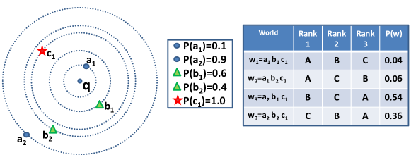
Figure 7: Example Database showing possible positions of uncertain objects and their corresponding probabilities.

Example 4

Figure 7 depicts a database containing objects $\mathcal{D}=\{A,B,C\}$. Objects $A$ and $B$ have two alternative locations each, while the position of $C$ is known for certain. The locations and the probabilities of all alternatives are also depicted in Figure 7. This leads to a total number of four possible worlds. For example, in world $w_{1}$ where $A=a_{1}$, $B=b_{1}$ and $C_{1}=c_{1}$, object $A$ is closest to $q$, followed by objects $B$ and $C$. Assuming inter-object independence, the probability of this world is given by the product of individual instance probabilities $P(w_{1})=P(a_{1})\cdot P(b_{1})\cdot P(c_{1})=0.04$. The ranking of each possible world and the corresponding probability is also depicted in Figure 7. For a probabilistic $2NN$ query for the depicted query object $q$, the object based result semantic computes the probability of each object to be in the two-nearest neighbor set of $q$. For object $A$, the probability $P(A)$ of this event equals $0.1$, since there exists exactly two possible worlds $w_{1}$ and $w_{2}$ with a total probability of $0.04+0.06=0.1$ in which $A$ is on rank one or on rank two, yielding a result tuple $(A,0.1)$. The complete result of a $P2NN$ query under object based result semantics is $\{(A,0.1),(B,0.94),(C,0.96)\}$. Note that in general, objects having a zero probability are included in the result. For instance, assume an additional object $D$ such that all instances of $D$ have a distance to $q$ greater than the distance between $q$ and $b_{2}$. In this case, the pair $(D,0)$ would be part of the result.

The result of a query under object based probabilistic result semantics contains one result tuple for every single database object, even if the probability of the corresponding object to be a result is very low or zero. In many applications, such results may be meaningless. Therefore, the size of the result set can be reduced by using a probabilistic query predicate as explained later in Section 6. A computational problem is the computation of the probability $P(o\in\mathcal{D})$ of an object $o$ to satisfy the spatial query predicate. In the example, this probability was derived by iterating over the set of all possible worlds $w_{1},...,w_{4}$. Since this set grows exponentially in the number of objects, such an approach is not viable in practice. Therefore, efficient techniques to compute the probability values $P(o)$ are required. A general paradigm to develop algorithms that avoid an explicit enumeration of all possible worlds is presented in Section 7.

5.2 Result Based Probabilistic Result Semantics

In the case of result based result semantics, possible result sets of a probabilistic spatial query are returned, each associated with the probability of this result.

Definition 4 (Result Based Result Semantics)

Let $\mathcal{D}$ be an uncertain spatial database, let $q$ be a query object and let $\phi$ denote a spatial query predicate. Under result based (RB) result semantics, the result of a probabilistic spatial $\phi$ query is a set

$$\phi_{RB}(q,\mathcal{D})=\{(r,P(r))|r\subseteq\mathcal{D},P(r)=\sum_{w\in\mathcal{W},\phi(q,w)=r}P(w)\}$$

of pairs. This set contains one pair for each result $r\subseteq\mathcal{D}$ associated with the probability $P(r)$ of $r$ to be the result. Following possible world semantics, the probability $P(r)$ is defined as the sum of probabilities of all worlds $w\in\mathcal{W}$ such that a spatial $\phi$ query returns $r$.

Formally, the result of a probabilistic spatial query under result based result semantics is a function

$$\phi_{RB}(q,\mathcal{D}):\overline{\mathcal{P}}(\mathcal{D})\rightarrow[0,1]$$

$$r\mapsto P(r).$$

mapping a elements of the power set $\overline{\mathcal{P}}(\mathcal{D})$ (the results) to probability values.

Example 5

For a probabilistic $2NN$ query for the depicted query object $q$, result based result semantics require to compute the probability of each subset of $\{A,B,C\}$ to be in the two-nearest neighbor set of $q$. For the set $\{B,C\}$, the probability of this event is $0.90$, since there is two possible worlds $w_{3}$ and $w_{4}$ with a total probability of $0.54+0.36=0.9$ in which $B$ and $C$ are both contained in the $2NN$ set of $q$. Note that in worlds $w_{3}$ and $w_{4}$ objects $B$ and $C$ appear in different ranking positions. This fact is ignored by a $kNN$ query, as the results are returned unsorted. In this example, the complete result of a $P2NN$ query under object based result semantics is $\{(\{A,B,C\},0)$, $(\{A,B\},0.04)$, $(\{A,C\},0.06)$, $(\{B,C\},0.90)$, $(\{A\},0)$, $(\{B\},0)$, $(\{C\},0)$, $(\{\emptyset\},0)\}$.

Clearly, the result of a query using result based result semantics can be used to derive the result of an identical query using object based result semantics. For instance, the result of Example 5 implies that the probability of object $A$ to be a $2NN$ of $q$ is $0.10$, since there exists two possible results using result based result semantics, namely $(\{A,B\},0.04)$ and $(\{A,C\},0.06)$ having a total probability of $0.04+0.06=0.1$, which matches the result of Example 4.

Lemma 1

Let $q$ be the query point of a probabilistic spatial $\phi$ query. It holds that the result of this query using object based result semantics $\phi_{OB}(q,\mathcal{D})$ is functionally dependent of the result of this query using result based result semantics. The set $PS\phi Q_{OB}(q,\mathcal{D})$ can be computed given only the set $PS\phi Q_{RB}(q,\mathcal{D})$ as follows:

$$PS\phi Q_{OB}(q,\mathcal{D})=\{(o,P(o))|o\in\mathcal{D}\wedge P(o)=\sum_{(r,P(r))\in PS\phi Q_{RB}(q,\mathcal{D}),o\in r}P(r)\}$$

Proof

Let $\mathcal{W}$ denote the set of possible worlds of $\mathcal{D}$, and let $p(w\in\mathcal{W})$ denote the probability of a possible world. Furthermore, let

$$w_{S\subseteq\mathcal{D}}:=\{w\in\mathcal{W}|\phi(q,w)=S\}$$

denote the set of possible worlds such that $\phi(q,w)=S$, i.e., such that the predicate that a $\phi$ query using query object $q$ returns set $S$ holds. In each world $w$, query $q$ returns exactly one deterministic result $PS\phi Q_{RB}(q,w)$. Thus, the sets $w_{S\subseteq\mathcal{D}}$ represent a complete and disjunctive partition of $\mathcal{W}$, i.e., it holds that

$$\mathcal{W}=\bigcup_{S\subseteq\mathcal{D}}w_{S}$$ (5)

and

$$\forall R,S\in\overline{\mathcal{P}}(\mathcal{D}):R\neq S\Rightarrow w_{R}\bigcap w_{S}=\emptyset.$$ (6)

Using Equations 5 and 6, we can rewrite Equation 4

$$P(o\in\phi_{OB}(q,\mathcal{D}))=\sum_{w\in\mathcal{W},o\in\phi(q,w)}P(w)$$

as

$$P(o\in\phi_{OB}(q,\mathcal{D}))=\sum_{S\in\overline{\mathcal{P}}(\mathcal{D})}\sum_{w\in w_{S},o\in\phi(q,w)}P(w).$$

By definition, query $q$ returns the same result for each world in $w\in w_{S}$. This result contains object $o$ if $o\in S$. Thus we can rewrite the above equation as

$$P(o)=\sum_{S\in\overline{\mathcal{P}}(\mathcal{D}),o\in S}P(S).$$

The probabilities $P(S)$ are given by function $PS\phi Q_{RB}(q,\mathcal{D})$.

In the above proof, we have performed a linear-time reduction of the problem of answering probabilistic spatial queries using object based result semantics to the problem of answering probabilistic spatial queries using result based result semantics. Thus, we have shown that, except for a linear factor (which can be neglected for most probabilistic spatial query types, since most algorithm run in no better than log-linear time), the problem of answering a probabilistic spatial query using result based result semantics is at least as hard as answering a probabilistic spatial query using object based semantics.

To summarize this section, we have learned about two different semantics to interpret the result of a spatial query on uncertain data: Object Based and Result Based. Understanding the difference of both result semantics is paramount to understand the landscape of existing research: in some related publication the problem of answering some probabilistic query may be proven to be in $\#P$, while another publication gives a solution that lies in $P$-TIME for the same spatial query predicate and the same probabilistic query predicate. In such cases, different result semantics may explain these results without assuming $P=NP$.

6 Probabilistic Query Predicates

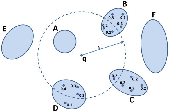
Figure 8: Example of an uncertain $\epsilon$-range query. Object $A$ is a true hit, objects $B$, $C$ and $D$ are possible hits.

Generally, in an uncertain database, the question whether an object satisfies a given query predicate $\phi$, such as being in a specified range or being a kNN of a query object, cannot be answered deterministically due to uncertainty of object locations. Due to this uncertainty, the predicate that an object satisfies $\phi$ is a random variable, having some (possibly zero, possibly one) probability. A probabilistic query predicate quantifies the minimal probability required for a result to qualify as a result that is sufficiently significant to be returned to the user. This section formally define probabilistic query predicate for general query predicates. The following definition are made for uncertain data in general, but can be applied analogously for uncertain spatial data.

A probabilistic query can be defined without any probabilistic query predicate. In this case, all objects, and their respective probabilities are returned.

Definition 5 (Probabilistic Query)

Let $\mathcal{D}$ be an uncertain database, let $q$ be a query point and let $\phi$ be a query predicate. A probabilistic query $\phi(q,\mathcal{D})$ returns all database objects $o\in\mathcal{D}$ together with their respective probability $P(o\in\phi(q,\mathcal{D}))$ that $o$ satisfies $\phi$.

$$\phi(q,\mathcal{D})=\{(o\in\mathcal{D},P(o\in\phi(q,\mathcal{D})))\}$$ (7)

The term probabilistic query is simply derived from the fact that unlike a traditional query, a probabilistic query result has probability values associated with each result. The main challenge of answering a probabilistic query, is to compute the probability $P(o\in\phi(q,\mathcal{D}))$ for each object. Using possible world semantics, a probabilistic query can be answered by evaluating the query predicate for each object and each possible world, i.e.,

$$P(o\in\phi(q,\mathcal{D})):=\sum_{w_{\in}\mathcal{W}f_{ind}(\phi,w)\cdot P(w)}.$$

But clearly, it is necessary to avoid the combinatorial growth that would be induced by this "naive" evaluation method.

Example 6

For example, consider the query “Return all friends of user $q$ having a spatial distance of less than $100m$ to $q$” depicted in Figure 8. Thus, the predicate $\phi$ is a $100$m-range predicate using query point $q$. We can deterministically tell that friend $A$ must be within $\epsilon=100m$ Euclidean distance of $q$, while friends $E$ and $F$ cannot possibly be in range. The pairs $(A,1)$, $(E,0)$ and $(F,0)$ are added to the result. For friends $B$, $C$ and $D$, this predicate cannot be answered deterministically. Here, friend $B$ has some possible positions located inside the $100m$ range of $q$, while other possible positions are outside this range. The two locations inside $q$’s range have a probability of $0.1$ and $0.2$, respectively, thus the total probability of object $B$ to satisfy the query predicate is $0.1+0.2=0.3$. The pair $(B,0.3)$ is thus added to the result. The pairs $(C,0.2)$ and $(D,0.9)$ complete the result $100\mbox{m-range}(q,\mathcal{D})=\{(A,1),(B,0.3),(C,0.2),(D,0.9),(E,0),(F,0)\}$.

The immediate question in the above example is:“Is a probability of $0.3$ sufficient to warrant returning $B$ as a result?”. To answer this question, a probabilistic query can explicitly specify a probabilistic query predicate, to specify the requirements, in terms of probability, required for an object to qualify to be included in the result. The following subsections briefly survey the most commonly used probabilistic query predicates: probabilistic threshold queries and probabilistic Top$k$ queries.

6.1 Probabilistic Threshold Queries

This paragraph defines a probabilistic query predicate that allows to return only results that are statistically significant.

Definition 6 (Probabilistic Threshold Query (P$\tau$Q))

Let $\mathcal{D}$ be an uncertain (spatial) database, let $q$ be a spatial query object, let $0\leq\tau\leq 1$ be a real value and let $\phi$ be a spatial query predicate. A probabilistic $\tau$ query (P$\tau$Q) returns all objects $o\in\mathcal{D}$ such that $o$ has a probability of at least $\tau$ to satisfy $\phi(q,\mathcal{D})$:

$$P\tau\phi(q,\mathcal{D}):=\{o\in\mathcal{D}|P(o\in\phi(q,\mathcal{D}))\geq\tau\}.$$

Example 7

In Figure 8, a probabilistic threshold $100m$-range(q,$\mathcal{D}$) query with $\tau=0.5$ query returns the set of objects $P0.5\,100\mbox{m-range}(q,\mathcal{D})=\{A,D\}$, since objects $A$ and $D$ are the only objects such that their total probability of alternatives inside the query region is equal or greater to $\tau=0.5$.

Semantically, a probabilistic threshold spatial query returns all results having a statistically significant probability to satisfy the query predicate. Therefore, the probabilistic threshold query serves as a statistical test of the hypothesis “o is a result” at a significance level of $\tau$. This test uses the probability $P(o\in\phi(q,\mathcal{D}))$ as a test statistic. Efficient algorithms to compute this probability $P(o\in\phi(q,\mathcal{D}))$, for the example of $k$NN and similarity ranking queries will be surveyed in Section 8 similarity ranking queries and R$k$NN queries.

A probabilistic threshold query on uncertain spatial data is useful in applications, where the parameters of the spatial predicate $\tau$ (e.g. the range of an $\epsilon$-range query, or the parameter $k$ of a $k$NN query), as well as the probabilistic threshold $\tau$ are chosen wisely, requiring expert knowledge about the database $\mathcal{D}$. If these parameters are chosen inappropriately, no results may be returned, or the set of returned result may grow too large. For example, if $\tau$ is chosen very large, and if the database has a high grade of uncertainty, then no result may be returned at all. Analogously, if the parameter $\epsilon$ is chosen too small then no result will be returned, while a too large value of $\epsilon$ may return all objects. The special case of having $\epsilon=0$, i.e., the case of returning all possible results (having a non-zero probability), is often used as default if no other probabilistic query predicate is specified (e.g. [97, 110]). This case may be referred to as a possibilistic query predicate, as all possible results (regardless of their probability) are returned.

6.2 Probabilistic Top$k$ Queries

In cases where insufficient information is given to select appropriate parameter values, the following probabilistic query predicate is defined to guarantee that only the $k$ most significant results are returned.

Definition 7 (Probabilistic Top$k$ Query (PTop$k$Q))

Let $\mathcal{D}$ be an uncertain spatial database, let $q$ be a spatial query object, let $1\leq k\leq|\mathcal{D}|$ be a positive integer, and let $\phi$ be a spatial query predicate. A probabilistic spatial Top$k$ query (PTop$k$Q) returns the smallest set PTop$k\phi$($q$,$\mathcal{D}$) of at least $k$ objects such that

$$\forall U_{i}\in\mbox{PTop}k\phi(q,\mathcal{D}),U_{j}\in\mathcal{D}\setminus\mbox{PTop}k\phi(q,\mathcal{D}):P(U_{i}\in\phi(q,\mathcal{D}))\geq P(U_{j}\in\phi(q,\mathcal{D}))$$

Thus, a probabilistic spatial Top$k$ query returns the $k$ objects having the highest probability to satisfy the query predicate. Again, in case of ties, the resulting set may be greater than $k$.

Example 8

In Figure 8, a PTop$3\,\phi$ query using a $\phi=100$m-range spatial predicate returns objects $PTop3\,100\mbox{m-range}(q,\mathcal{D})=\{A,B,D\}$, since these objects have the highest probability to satisfy the spatial predicate, i.e., have the highest probability to be located in the spatial $100m$-range.

Note, that the probabilistic Top$k$ query predicate can be combined with a $kNN$ spatial query, i.e., with the case where $\phi=kNN$. Such a probabilistic Top$k$ $jNN$ query returns the set of $k$ objects having the highest probability, to be $j$-nearest neighbor of the query object. Clearly, $k$ and $j$ may have different integer values, such that differentiation is needed.

6.3 Discussion

In summary, a probabilistic spatial query is defined by two query predicates:

• A spatial predicate $\phi$ to select uncertain objects having sufficiently high proximity to the query object, and

• a probabilistic predicate $\psi$, to select uncertain objects having sufficiently high probability to satisfy $\phi$.

It has to be mentioned, that alternatively to this definition, a single predicate can be used, that combines both spatial and probabilistic features. For example, a monotonic score function can be utilized, which combines spatial proximity and probability to return a single scalar score. An example of such a monotone score function is the expected distance function

$$E(dist(q,U\in\mathcal{D}))=\sum_{u\in U}P(u)\cdot dist(q,u),$$

where $q$ is the query object, and $\mathcal{D}$ is an uncertain database. The expected support function is utilized by a number of related publications, such as [78, 37]. Using such a monotone score function, objects with a sufficiently high score can be returned. The advantage of using such an approach, is that objects that are located very close to the query require a lower probability to be returned as a result, while objects that are located further away from the query object require a higher probability. Yet, the main problem of such a combined predicate, is that the probability of an object is treated as a simple attribute, thus losing its probabilistic semantic. Thus, the resulting score is very hard to interpret. An object that has a high score, may indeed have a very low probability to exist at all, because it is located (if it exists) very close to the query object. Consequently, the score itself no longer contains any confidence information, and thus, it is not possible to answer queries according to possible world semantics using a single aggregate, such as expected distance, only.

7 The Paradigm of Equivalent Worlds

In Section 3 the concept of possible world semantics has been introduced. Possible world semantics give an intuitive and mathematically sound interpretation of an uncertain spatial database. Furthermore, queries that adhere to possible world semantics return unbiased results, by evaluating the query on each possible world. Since any such approach requires to run queries on an exponential number of worlds, any naive approach is infeasible. Yet, for specific settings, such as specific result-based semantics, specific spatial query predicates and specific probabilistic query predicates, the literature has shown that it is possible to efficiently answer queries on uncertain data. While it is hardly feasible to enumerate all combinations of result-based semantics, spatial query predicates and probabilistic query predicates, this section introduces a general paradigm to find such a solution yourself. In a nutshell, the idea is to find, among the exponentially large set of possible worlds, a partitioning into a polynomially large number of subsets, which are equivalent for a given query.

7.1 Equivalent Worlds

The goal of this section is introduce a general paradigm to efficiently compute exact probabilities, while still adhering to possible world semantics. For this purpose, reconsider Definition 2, defining the probability that some predicate $\phi$ is satisfied in an uncertain database $\mathcal{D}$ as the total probability of all possible worlds satisfying $\phi$. Recall Equation 3

$$P(\phi(\mathcal{D}))=\sum_{w\in\mathcal{W}}\mathcal{I}(\phi,w)\cdot P(w),$$

where $\mathcal{W}$ is the set of all possible worlds; $\mathcal{I}(\phi,w)$ is an indicator function that returns one if predicate $\phi$ holds (i.e., resolves to true) in the crisp database defined by world $w$ and zero otherwise, and $P(w)$ is the probability of world $w$. To reduce the number of possible worlds that need to be considered to compute $P(\phi(\mathcal{D}))$, we first need the following definition.

Definition 8 (Class of Equivalent Worlds)

Let $\phi$ be a query predicate and let $S\subseteq\mathcal{W}$ be a set of possible worlds such that for any two worlds $w_{1},w_{2}\in S$ we can guarantee that $\phi$ holds in world $w_{1}$ if an only if $\phi$ holds in world $w_{2}$, i.e.,

$$\forall w_{1},w_{2}\in S:\mathcal{I}(\phi,w_{1})\Leftrightarrow\mathcal{I}(\phi,w_{2})$$

Then set $S$ is called a class of worlds equivalent with respect to $\phi$. In the remainder of this chapter, if the spatial query predicate $\phi$ is clearly given by the context, then $S$ will simply be denoted as a class of equivalent worlds. Any worlds $w_{i},w_{j}\in S$ are denoted as equivalent worlds.

We now make the following observation:

Corollary 1

Let $S\subseteq\mathcal{W}$ be a class of worlds equivalent with respect to $\phi$ (c.f. Definition 8, we can rewrite Equation 3 as follows:

$$P(\phi(\mathcal{D}))=\sum_{w\in\mathcal{W}}\mathcal{I}(\phi,w)\cdot P(w)\Leftrightarrow$$

$$P(\phi(\mathcal{D}))=\sum_{w\in\mathcal{W}\setminus S}\mathcal{I}(\phi,w)\cdot P(w)+\mathcal{I}(\phi,w\in S)\cdot\sum_{w\in S}P(w).$$ (8)

Proof

Due to the assumption that for any two worlds $w_{1},w_{2}\in S$ it holds that $\phi$ holds in world $w_{1}$ if an only if $\phi$ holds in world $w_{2}$, we get $\mathcal{I}(\phi,w_{1})=1\Leftrightarrow\mathcal{I}(\phi,w_{2})=1$ and $\mathcal{I}(\phi,w_{1})=0\Leftrightarrow\mathcal{I}(\phi,w_{2})=0$ by definition of function $\mathcal{I}$. Due to this assumption, we have to consider two cases.

Case 1: $\forall w\in S:\mathcal{I}(\phi,w)=0$

In this case, both Equation 3 and Equation 8 can be rewritten as

$$P(\phi(\mathcal{D}))=\sum_{w\in\mathcal{W}\setminus S}\mathcal{I}(\phi,w)\cdot P(w).$$

Case 2: $\forall w\in S:\mathcal{I}(\phi,w)=1$

In this case, both Equation 3 and Equation 8 can be rewritten as

$$P(\phi(\mathcal{D}))=\sum_{w\in\mathcal{W}\setminus S}\mathcal{I}(\phi,w)\cdot P(w)+\sum_{w\in S}P(w)$$

∎

The only difference between both cases is the additive term $\sum_{w\in S}P(w)$, which exists only in Case 2. The indicator function $\mathcal{I}(\phi,w\in S)$ ensures that this term is only added in the second case. As main purpose, Corollary 1 states that, given a set of equivalent worlds $S$, we only have to evaluate the indictor function $\mathcal{I}(\phi,w)$ on a single representative world $w\in S$, rather than on each world in $S$. This allows to reduce the number of (crisp) $\phi$ queries required to compute Equation 3 by $|S|-1$.

Corollary 1 leads to the following Lemma.

Lemma 2

Let $\mathcal{S}$ be a partitioning of $\mathcal{W}$ into disjoint sets such that $\bigcup_{S\in\mathcal{S}}S=\mathcal{W}$ and for all $S_{1},S_{2}\in\mathcal{S}:S_{1}\cap S_{2}=\emptyset$. Equation 3 can be rewritten as

$$P(\phi(\mathcal{D}))=\sum_{w\in\mathcal{W}}\mathcal{I}(\phi,w)\cdot P(w)\Leftrightarrow$$

$$P(\phi(\mathcal{D}))=\sum_{S\in\mathcal{S}}\mathcal{I}(\phi,w\in S)\cdot\sum_{w\in S}P(w).$$ (9)

Proof

Lemma 2 is derived by applying Corollary 1 once for each $S\in\mathcal{S}$.∎

The next subsection will show how to leverage Lemma 2 to partition the set of all possible worlds into equivalence classes that are guaranteed to have the same result for a given query predicate, and how to exploit this partitioning to efficiently answer queries.

7.2 Exploiting Equivalent Worlds for Efficient Algorithms

Given a partitioning $\mathcal{S}$ of all possible worlds, Equation 9 requires to perform the following two tasks. The first task requires to evaluate the indicator function $\mathcal{I}(\phi,w\in S)$ for one representative world of each partition. This can be achieved by performing a traditional (non-uncertain) $\phi$ query on these representatives. The final challenge is to efficiently compute the total probability $P(S):=\sum_{w\in S}P(w)$ for each equivalent class $S\in\mathcal{S}$. This computation must avoid an enumeration of all possible worlds, i.e., must be in $o(|S|)$. Achieving an efficient computation is a creative task, and usually requires to exploit properties of the model (such as object independence) and properties of the spatial query predicate.

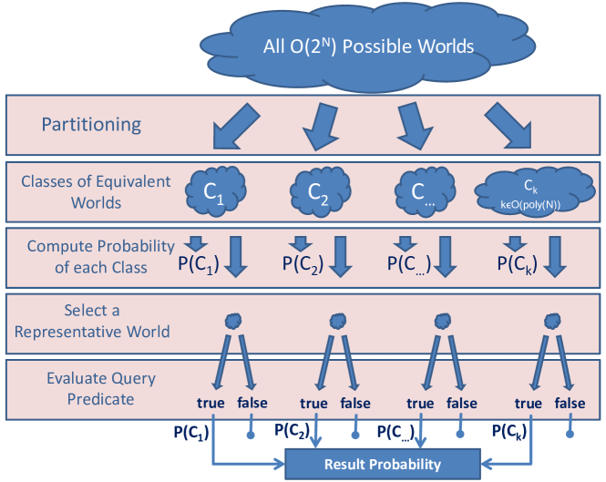
Figure 9: Summary of the Paradigm of Equivalent Worlds.

The paradigm of equivalent worlds is illustrated and summarized in Figure 9. In the first step, set of all possible worlds $\mathcal{W}$, which is exponential in the number $N$ of uncertain objects, has to be partitioned into a polynomial large set of classes of equivalent worlds, such that all worlds in the same class are guaranteed to be equivalent given the query predicate $\phi$. This yields a the set $\mathcal{C}=\{C_{1},C_{2},...,C_{k}\}$ of classes of equivalent worlds. To allow efficient processing, this set must be polynomial in size, since each class has to be considered individually in the following. Next, we require to compute the probability of each class $C_{i}$, without enumeration of all possible worlds contained in $C_{i}$, the number of which may still be exponential. In fact, at least one class $C_{i}$ must contain $O(2^{N})$ possible worlds. Next, we need to decide, for each class $C_{i}$, whether all worlds $w\in C_{i}$ satisfy the query predicate $\phi$, or whether no world $w\in C_{i}$ satisfies $\phi$. Due to equivalence of all possible worlds in $C_{i}$, these are the only possible cases. For some query predicates, this decision can be made using special properties of the query predicate, as we will see later in this chapter. In the general case, this decision can be made by choosing one representative world $w\in C_{i}$ (e.g. at random) from each class $C_{i}$, and evaluating the query predicate on this world. This yields at total run-time of $O(|\mathcal{C}|)\cdot O(\mathcal{I}(\phi,w))$, where $\mathcal{I}(\phi,w)$ is the time complexity of evaluating the query predicate $\phi$ on the certain database $w$. If this query predicate can be evaluated in polynomial time, i.e., if $O(\mathcal{I}(\phi,w))\in O(poly(N))$, then the total run-time is in $O(poly(N))$. This is evident, since if $O(\mathcal{C})$ is in $O(poly(N))$, then $O(\mathcal{C})\cdot O(\mathcal{I}(\phi,w))$ is in $O(poly(N))\cdot O(poly(N))$ which is in $O(poly(N))$. For each class $C_{i}$, where the representative world satisfies $\phi$, the corresponding probability $P(C_{i})$ is added to the result probability.

The following lemma summarizes the assumptions that a query predicate has to satisfy in order to efficiently apply paradigm of finding equivalent worlds.

Lemma 3

Given a query predicate $\phi$ and an uncertain database $\mathcal{D}$ of size $N:=|DB|$, we can answer $\phi$ on $\mathcal{D}$ in polynomial time if the following four conditions are satisfied:

• A traditional $\psi$ query on non-uncertain data can be answered in polynomial time.

• we can identify a partitioning $\mathcal{C}$ of $\mathcal{W}$ into classes $C\in\mathcal{C}$ of equivalent worlds (see Definition 8.

• The number $|\mathcal{C}|$ of classes is at most polynomial in $N$.

• The the total probability of a class $S\in\mathcal{C}$ can be computed in at most polynomial time.

Proof

Answering a $\phi$ query on $\mathcal{D}$ requires to evaluate Equation 3 which we reformed into Equation 9 using Property II. This requires to iterate over all $|\mathcal{C}|$ classes of equivalent worlds in polynomial time due to Property III. For each class $C\in\mathcal{C}$, this requires to perform two tasks. The first task requires to compute the total probability of all worlds in $C$, and the second task requires to evaluate $\phi$ on a single possible world $w\in C$. The former task can be performed in polynomial time due to Property IV. The later task requires to perform a crisp $\phi$ query on the (crisp) world $w$ in polynomial time due to Property I.

8 Case Study: Range Queries and the Sum of Independent Bernoulli Trials

In this chapter, the paradigm of equivalent worlds will be applied to efficiently solve the problem of computing the number of uncertain objects located within a specified range.

Example 9

As an example, consider the setting depicted in Figure 8. In this example, we have four objects, $A$, $B$, $C$, and $D$ having probabilities of $1.0$, $0.3$, $0.2$, and $0.9$ of being located inside the query region defined by query location $q$ and query range $\epsilon$. Intuitively, the number of objects in this range can be anywhere between one and four, as only object $A$ is guaranteed to be inside the range, while on $B$, $C$, and $D$ have a chance to be inside this range among all other objects. How can we efficiently compute the distribution of this number of objects inside the query range? What is the probability of having exactly one, two, three or four object in the range? Intuitively, the number of objects corresponds depends on the result of three “coin-flips”, each using a coin with a different bias of flipping heads.

Each such “coin-flip” is a Bernoulli trial, which may have a successful (“heads”) of unsuccessful (“tails”) outcome. In the case where all Bernoulli trials have the same probability $p$, the number of successful trials out of $N$ trials is described by the well-known binomial distribution. In the case where each trial may have a different probability to succeed, the number of successful trials follows a Poisson-binomial distributions [55].

Formally, let $X_{1},...,X_{N}$ be independent and not necessarily identically distributed Bernoulli trials, i.e., random variables that may only take values zero and one. Let $p_{i}:=P(X_{i}=1)$ denote the probability that random variable $X_{i}$ has value one. In this section, we will show how to efficiently compute the distribution of the random variable

$$\sum_{i=1}^{N}X_{i}$$

without enumeration of all possible worlds. That is, for each $0\leq k\leq N$, this section shows how to compute the probability $P(\sum_{i=1}^{N}X_{i}=k)$ that exactly $k$ trials are successful.

This section shows two commonly used solutions to compute the distribution of $\sum_{i}X_{i}$ efficiently: The Poisson-binomial recurrence, and a technique based on generating functions. Both solutions have in common that they identify worlds that are equivalent to the query predicate.

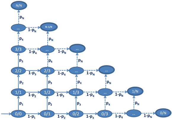
Figure 10: Deterministic finite automaton corresponding to the problem of the sum of independent Bernoulli trials.

8.1 Poisson-Binomial Recurrence

The first approach iteratively computes the distribution of the sum of the first $1\leq k\leq N$ Bernoulli variables given the distribution of the sum of the first $k-1$ Bernoulli variables.

To gain an intuition of how to do this efficiently, consider the deterministic finite automaton depicted in Figure 10. The states (i/j) of this automaton correspond to the random event that out of the first $j$ Bernoulli trials $X_{1},...,X_{j}$, exactly $i$ trials have been successful. Initially, zero Bernoulli trials have been performed, out of which zero (trivially) were successful. This situation is represented by the initial state $(0/0)$ in Figure 10. Evaluating the first Bernoulli trial $X_{1}$, there is two possible outcomes: The trial may be successful with a probability of $p_{1}$, leading to a state $(1/1)$ where one out of one trials have been successful. Alternatively, the trial may be unsuccessful, with a probability of $1-p_{1}$, leading to a state $(0/1)$ where zero out of one trial have been successful. The second trial is then applied to both possible outcomes. If the first trial has not been successful, i.e., we are currently located in state $(0/1)$, then there is again two outcomes for the second Bernoulli trial, leading to state $(1/2)$ and $(0/2)$ with a probability of $p_{2}$ and $1-p_{2}$ respectively. If currently located in state $(0/1)$, the two outcomes are state $(2/2)$ and state $(1/2)$ with the same probabilities. At this point, we have unified two different possible worlds that are equivalent with respect to $\sum_{i}X_{i}$: The world where trial one has been successful and trial two has not been successful, and the world where trial one has not been successful and trial two has been successful have been unified into state $(1/2)$, representing both worlds. This unification was possible, since both paths leading to state $(1/2)$ are equivalent with respect to the number of successful trials.

The three states $(0/2)$, $(1/2)$ and $(2/2)$ are then subjected to the outcome of the third Bernoulli trial, leading to states $(0/3)$, $(1/3)$, $(2/3)$ and $(3/3)$. That is a total of four states for a total of $2^{3}=8$ possible worlds. In summary, the number of states in Figure 10 equals $\frac{N^{2}}{2}$. However, it is not yet clear how to compute the probability of a state $(i/j)$ efficiently. Naively, we have to compute the sum over all paths leading to state $(i/j)$. For example, the probability of state (2/3) is given by $p_{1}\cdot p_{2}\cdot(1-p_{3})+p_{1}\cdot(1-p_{2})\cdot p_{3}+(1-p_{1})\cdot p_{2}\cdot p_{3}$. This naive computation requires to enumerate all $\binom{j}{p_{3}}$ combinations of paths leading to state $(i/j)$.

For an efficient computation, we make the following observation: Each state of the deterministic finite automaton depicted in Figure 10 has at most two incoming edges. Thus, to compute the probability of a state $(i/j)$, we only require the probabilities of states leading to $(i/j)$. The states leading to state $(i/j)$ are state $(i-1/j-1)$ and state $(i/j-1)$. Given the probabilities $P(i-1/j-1)$ and $P(i/j-1)$, we can compute the probability $P(i/j)$ of state (i/j) as follows:

$$P(i/j)=P(i-1/j-1)\cdot p_{j}+P(i,j-1)\cdot(1-p_{j})$$ (10)

where

$$P(0/0)=1\mbox{ and }P(i/j)=0\mbox{ if }i>j\mbox{ or if }i<0.$$

Equation 10 is known as the Poisson-Binomial Recurrence (To the best of our knowledge, the Poisson binomial recurrence was first introduced by [65]) and can be used to compute the probabilities of states $(k/N),0\leq k\leq N$ which by definition, correspond to the probabilities $P(\sum_{i=1^{N}}X_{i}=k)$ that out of all $N$ Bernoulli trials, exactly $k$ trials are successful.

This approach follows the paradigm of equivalent worlds in each iteration $k$: The set of all $2^{k}$ possible worlds is partitioned into $k+1$ equivalent sets, each corresponding to a state $i/k$, where $i\leq k$. Each class contains only and all of the $\binom{k}{i}$ possible worlds where exactly $i$ Bernoulli trails succeeded. The information about the particular sequence of the successful trials, i.e., which trials were successful and which were unsuccessful is lost. This information however, is no longer necessary to compute the distribution of $\sum_{i=0}^{N}X_{i}$, since for this random variable, we only need to know the number of successful trials, not their sequence. This abstraction allows to remove the combinatorial aspect of the problem.

An example showcasing the Poisson binomial recurrence is given in the following.

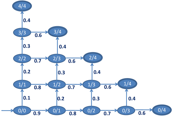
Figure 11: Deterministic finite automaton for four Bernoulli random variables.

Example 10

Let $N=4$ and let $p_{1}=0.1$, $p_{2}=0.2$, $p_{3}=0.3$ and $p_{4}=0.4$. The corresponding DFA is depicted in Figure 11. The probability of state (0/0) is explicitly set to $1.0$ in Equation 10. To compute the probability of state (0/1), we apply Equation 10 to compute

$$P(0/1)=P(-1/0)\cdot p_{1}+P(0/0)\cdot(1-p_{1}).$$

with $P(-1/0)=0$ and $P(0/0)=1$ explicitly defined in Equation 10 this yields

$$P(0/1)=0\cdot p_{1}+1\cdot(1-p_{1})=0.9$$

Analogously, we obtain

$$P(1/1)=P(0/0)\cdot p_{1}+P(1/0)\cdot(1-p_{1})=1\cdot p_{1}=0.1$$

Using these initial probabilities, we can continue to compute

$$P(0/2)=P(-1/1)\cdot p_{2}+P(0/1)\cdot(1-p_{2})=0\cdot 0.2+0.9\cdot 0.8=0.72$$

$$P(1/2)=P(0/1)\cdot p_{2}+P(1/1)\cdot(1-p_{2})=0.9\cdot 0.2+0.1\cdot 0.8=0.26$$

$$P(2/2)=P(1/1)\cdot p_{2}+P(2/1)\cdot(1-p_{2})=0.1\cdot 0.2+0\cdot 0.8=0.02$$

The probabilities $P(i/2),0\leq i\leq 2$ can be used to compute

$$P(0/3)=P(-1/2)\cdot p_{3}+P(0/2)\cdot(1-p_{3})=0\cdot 0.3+0.72\cdot 0.7=0.504$$

$$P(1/3)=P(0/2)\cdot p_{3}+P(1/2)\cdot(1-p_{3})=0.72\cdot 0.3+0.26\cdot 0.7=0.398$$

$$P(2/3)=P(1/2)\cdot p_{3}+P(2/2)\cdot(1-p_{3})=0.26\cdot 0.3+0.02\cdot 0.7=0.092$$

$$P(3/3)=P(2/2)\cdot p_{3}+P(3/2)\cdot(1-p_{3})=0.02\cdot 0.3+0\cdot 0.7=0.006$$

Finally, these probabilities can be used to derive the final distribution of the random variable $\sum_{i=1}^{4}X_{i}$:

$$P(0/4)=P(-1/3)\cdot p_{4}+P(0/3)\cdot(1-p_{4})=0\cdot 0.4+0.504\cdot 0.6=0.3024$$

$$P(1/4)=P(0/3)\cdot p_{4}+P(1/3)\cdot(1-p_{4})=0.504\cdot 0.4+0.398\cdot 0.6=0.4404$$

$$P(2/4)=P(1/3)\cdot p_{4}+P(2/3)\cdot(1-p_{4})=0.398\cdot 0.4+0.092\cdot 0.6=0.2144$$

$$P(3/4)=P(2/3)\cdot p_{4}+P(3/3)\cdot(1-p_{4})=0.092\cdot 0.4+0.006\cdot 0.6=0.0404$$

$$P(4/4)=P(3/3)\cdot p_{4}+P(4/3)\cdot(1-p_{4})=0.006\cdot 0.4+0\cdot 0.6=0.0024$$

These probabilities describe the PDF of $\sum_{i=1}^{4}X_{i}$ by definition of $P(i/j)$.

Complexity Analysis

To compute the distribution of $\sum_{i}X_{i}$ we require to compute each probability $P(i/j)$ for $0\leq j\leq N,i\leq j$, yielding a total of $\frac{N^{2}}{2}\in O(N^{2})$ probability computations. To compute any such probability, we have to evaluate Equation 10, which requires to look up four probabilities $P(i-1/j-1)$, $P(i/j-1)$, $p_{j}$ and $1-p_{j}$, which can be performed in constant time. This yields a total runtime complexity of $O(N^{2})$. The $O(N^{2})$ space complexity required to store the matrix of probabilities $P(i/j)$ for $0\leq j\leq N,i\leq j$ can be reduced to $O(N\cdot k)$ by exploiting that in each iteration where the probabilities $P(i/k),0\leq i\leq k$ are computed, only the probabilities $P(i/k-1),0\leq i\leq k-1$ are required, and the result of previous iterations can be discarded. Thus, at most $N$ probabilities have to be stored at a time.

8.2 Generating Functions

An alternative technique to compute the sum of independent Bernoulli variables is the generating functions technique. While showing the same complexity as the Poisson binomial recurrence, its advantage is its intuitiveness.

Represent each Bernoulli trial $X_{i}$ by a polynomial $poly(X_{i})=p_{i}\cdot x+(1-p_{i})$. Consider the generating function

$$\mathcal{F}^{N}=\prod_{i=1}^{N}poly(X_{i})=\sum_{i=0}^{N}c_{i}x^{i}.$$ (11)

The coefficient $c_{i}$ of $x^{i}$ in the expansion of $\mathcal{F}^{N}$ equals the probability $P(\sum_{n=1}^{N}X_{n}=i)$ ([66]). For example, the monomial $0.25\cdot x^{4}$ implies that with a probability of $0.25$, the sum of all Bernoulli random variables equals four.

The expansion of $N$ polynomials, each containing two monomials leads to a total of $2^{N}$ monomials, one monomial for each sequence of successful and unsuccessful Bernoulli trials, i.e., one monomial for each possible worlds. To reduce this complexity, again an iterative computation of $\mathcal{F}^{N}$, can be used, by exploiting that

$$\mathcal{F}^{k}=\mathcal{F}^{k-1}\cdot poly(X_{k}).$$ (12)

This rewriting of Equation 11 allows to inductively compute $\mathcal{F}^{k}$ from $\mathcal{F}^{k-1}$. The induction is started by computing the polynomial $\mathcal{F}^{0}$, which is the empty product which equals the neutral element of multiplication, i.e., $\mathcal{F}^{0}=1$. To understand the semantics of this polynomial, the polynomial $\mathcal{F}^{0}=1$ can be rewritten as $\mathcal{F}^{0}=1\cdot x^{0}$, which we can interpret as the following tautology:“with a probability of one, the sum of all zero Bernoulli trials equals zero.” After each iteration, we can unify monomials having the same exponent, leading to a total of at most $k+1$ monomials after each iteration. This unification step allows to remove the combinatorial aspect of the problem, since any monomial $x^{i}$ corresponds to a class of equivalent worlds, such that this class contains only and all of the worlds where the sum $\sum_{k=1}^{N}X_{k}=1$. In each iteration, the number of these classes is $k$ and the probability of each class is given by the coefficient of $x^{i}$.

An example showcasing the generating functions technique is given in the following. This examples uses the identical Bernoulli random variables used in Example 10.

Example 11

Again, let $N=4$ and let $p_{1}=0.1$, $p_{2}=0.2$, $p_{3}=0.3$ and $p_{4}=0.4$. We obtain the four generating polynomials $poly(X_{1})=(0.1x+0.9)$, $poly(X_{2})=(0.2x+0.8)$, $poly(X_{3})=(0.3x+0.7)$, and $poly(X_{4})=(0.4x+0.6)$. We trivially obtain $\mathcal{F}^{0}=1$. Using Equation 12 we get

$$\mathcal{F}^{1}=\mathcal{F}^{0}\cdot poly(X_{1})=1\cdot(0.1x+0.9)=0.1x+0.9.$$

Semantically, this polynomial implies that out of the first one Bernoulli variables, the probability of having a sum of one is $0.1$ (according to monomial $0.1x=0.1x^{1}$, and the probability of having a sum of zero is $0.9$ (according to monomial $0.9=0.9x^{0}$. Next, we compute $F^{2}$, again using Equation 12:

$$\mathcal{F}^{2}=\mathcal{F}^{1}\cdot poly(X_{2})=(0.1x^{1}+0.9x^{0})\cdot(0.2x^{1}+0.8x^{0})=$$

$$0.02x^{1}x^{1}+0.08x^{1}x^{0}+0.18x^{0}x^{1}+0.72x^{0}x^{0}$$

In this expansion, the monomials have deliberately not been unified to give an intuition of how the generating function techniques is able to identify and unify equivalent worlds. In the above expansion, there is one monomial for each possible world. For example, the monomial $0.18x^{0}x^{1}$ represents the world where the first trial was unsuccessful (represented by the zero of the first exponent) and the second trial was succesful (represented by the one of the second exponent). The above notation allows to identify the sequence of successful and unsuccessful Bernouli trials, clearly leading to a total of $2^{k}$ possible worlds for $\mathcal{F}^{k}$. However, we know that we only need to compute the total number of successful trials, we do not need to know the sequence of successful trials. Thus, we need to treat worlds having the same number of successful Bernoulli trials equivalently, to avoid the enumeration of an exponential number of sequences. This is done implicitly by polynomial multiplication, exploiting that

$$0.02x^{1}x^{1}+0.08x^{1}x^{0}+0.18x^{0}x^{1}+0.72x^{0}x^{0}=0.02x^{2}+0.08x^{1}+0.18x^{1}+0.72x^{0}$$

This representation no longer allows to distinguish the sequence of successful Bernouli trials. This loss of information is beneficial, as it allows to unify possible worlds having the same sum of Bernoulli trials.

$$0.02x^{2}+0.08x^{1}+0.18x^{1}+0.72x^{0}=0.02x^{2}+0.26x^{1}+0.72x^{0}$$

The remaining monomials represent an equivalence class of possible worlds. For example, monomial $0.26x^{1}$ represents all worlds having a total of one successful Bernoulli trials. This is evident, since the coefficient of this monomial was derived from the sum of both worlds having a total of one successful Bernoulli trials.In the next iteration, we compute:

$$\mathcal{F}^{3}=\mathcal{F}^{2}\cdot poly(X_{3})=(0.02x^{2}+0.26x^{1}+0.72x^{0})\cdot(0.3x+0.7)$$

$$=0.006x^{2}x^{1}+0.014x^{2}x^{0}+0.078x^{1}x^{1}+0.182x^{1}x^{0}+0.216x^{0}x^{1}+0.504x^{0}x^{0}$$

This polynomial represents the three classes of possible worlds in $\mathcal{F}^{2}$ combined with the two possible results of the third Bernoulli trial, yielding a total of $3\dot{2}$ monomials. Unification yields

$$0.006x^{2}x^{1}+0.014x^{2}x^{0}+0.078x^{1}x^{1}+0.182x^{1}x^{0}+0.216x^{0}x^{1}+0.504x^{0}x^{0}=$$

$$0.006x^{3}+0.092x^{2}+0.398x^{1}+0.504$$

The final generating function is given by

$$\mathcal{F}^{4}=\mathcal{F}^{3}\cdot poly(X_{4})=$$

$$(0.006x^{3}+0.092x^{2}+0.398x^{1}+0.504)\cdot(0.4x+0.6)=$$

$$.0024x^{4}+.0036x^{3}+.0368x^{3}+.0552x^{2}+.1592x^{2}+.2388x^{1}+.2016x^{1}+.3024x^{0}$$

$$=0.0024x^{4}+0.0404x^{3}+0.2144x^{2}+0.4404x+0.3024$$

This polynomial describes the PDF of $\sum_{i=1}^{4}X_{i}$, since each monomial $c_{i}x^{i}$ implies that the probability, that out of all four Bernoulli trials, the total number of successful events equals $i$, is $c_{i}$. Thus, we get $P(\sum_{i=1}^{4}X_{i}=0)=0.0024$, $P(\sum_{i=1}^{4}X_{i}=1)=0.0404$, $P(\sum_{i=1}^{4}X_{i}=2)=0.2144$, $P(\sum_{i=1}^{4}X_{i}=3)=0.4404$ and $P(\sum_{i=1}^{4}X_{i}=4)=0.3024$. Note that this result equals the result we obtained by using the Poisson binomial recurrence in the previous section.

Complexity Analysis

The generating function technique requires a total of $N$ iterations. In each iteration $1\leq k\leq N$, a polynomial of degree $k$, and thus of maximum length $k+1$, is multiplied with a polynomial of degree $1$, thus having a length of $2$. This requires to compute a total of $(k+1)\cdot 2$ monomials in each iteration, each requiring a scalar multiplication. Thus leads to a total time complexity of $\sum_{i=1}^{N}2k+2\in O(N^{2})$ for the polynomial expansions. Unification of a polynomial of length $k$ can be done in $O(k)$ time, exploiting that the polynomials are sorted by the exponent after expansion. Unification at each iteration leads to a $O(n^{2})$ complexity for the unification step. This results in a total complexity of $O(n^{2})$, similar to the Poisson binomial recurrence approach.

An advantage of the generating function approach is that this naive polynomial multiplication can be accelerated using Discrete Fourier Transform (DFT). This technique allows to reduce to total complexity of computing the sum of $N$ Bernoulli random variables to $O(Nlog^{2}N)$ ([71]). This acceleration is achieved by exploiting that DFT allows to expand two polynomials of size $k$ in $O(klogk)$ time. Equi-sized polynomials are obtained in the approach of [71], by using a divide and conquer approach, that iteratively divides the set of $N$ Bernoulli trials into two equi-sized sets. Their recursive algorithm then combines these results by performing a polynomial multiplication of the generating polynomials of each set. More details of this algorithm can be found in [71].

9 Advanced Techniques for Managing Uncertain Spatial Data

Table 2: Advanced Topics in Querying and Mining Uncertain Spatial Data.

Topic	Related Work
Nearest Neighbor Query Processing	[33, 61, 29, 58, 115, 82, 93]
$k$-Nearest Neighbor ($k$NN) Query Processing	[60, 21, 30, 15]
Top-$k$ Query Processing	[88, 97, 111]
Ranking of Uncertain Spatial Data	[74, 19, 37, 96, 70, 18, 39, 76, 17, 57]
Reverse $k$NN Query Processing	[75, 27, 16, 46]
Skyline Query Processing	[87, 73, 103, 45, 109]
Indexing Uncertain Spatial Data	[114, 47, 1]
Maximum Range-Sum Query Processing	[2, 80, 77]
Querying Uncertain Trajectory Data	[48, 83, 117]
Clustering Uncertain Spatial Data	[94, 120, 81, 62]
Frequent Itemset and Colocation Mining	[14, 106, 20, 17, 107]

The Paradigm of Equivalent worlds has been successfully applied to efficiently support many spatial query predicates and spatial data mining tasks. These more advanced techniques are out of scope of this book chapter, but the techniques presented in this chapter should help the interested reader to dive deeper into understanding state-of-the-art solutions, and to help the reader to contribute to this field. An overview of research directions on uncertain spatial is provided in Table 2.

Efficient solutions on uncertain data have been presented for ($1$)-nearest neighbor ($1$NN) queries [33, 61, 29, 58, 115, 82, 93]. The case of $1NN$ is special, as for $1NN$ the cases of object-based and result-based probabilistic result semantics are equivalent: Since a $1NN$ query only results a single result object. Thus, the probability of any object to be part of the result is equal the probability of this object to be the (whole) result. For $k$ Nearest Neighbor queries, this is not the case, as initially motivated in Figure 2. For object-based result semantics (as explained in Section 5), polynomial time solutions leveraging the paradigm of equivalent worlds have been proposed [15]. For result-based result semantics, where each of the (potentially exponential many in $k$) results is associated with a probability, solutions have been presented in [21, 30].

A related problem is Top-$k$ query processing which returns the $k$ best result objects for a given score function [88, 97, 111]. While these solution are not proposed in the context of spatial or spatio-temporal data, they are mentioned here as they can be applied to spatial data. For example, if the score function is defined as the distance to query object, this problem becomes equivalent to $k$NN. Solutions for result-based probabilistic result semantics are proposed in [97, 88] and for object-based result semantics in [111].

Another problem generalization are ranking queries, which return the Top-$k$ result ordered by score. For uncertain data using object-based result semantics, this yields a probabilistic mapping of each database mapping to each rank for the case of object-based result semantics. For example, it may return that object $o_{1}$ has a $80\%$ probability to be Rank 1, and a $20\%$ probability to be Rank 2. In the case of result-based probabilistic result semantics, each possible ranking of objects is mapped to a probability, for example, the ranking $[o_{1},o_{3},o_{2}]$ may have a $10\%$ probability. Solutions for the result-based probabilistic result semantic case have been proposed in [96] having exponential run-time due to the hard nature of this problem. For the case of object-based probabilistic result semantics, first solutions having exponential run-time were proposed [19, 74]. Applying the paradigm of equivalent worlds, a number of solutions have been proposed concurrently and independently to achieve polynomial run-time (linear in the number of database objects times the number of ranks). The generating functions technique (as explained in Section 8) was proposed for this purpose by Li et al. [70]. An equivalent approach using a technique called Poisson-Binomial Recurrence was simultaneously proposed by [18, 57]. A comparison of the generating functions technique and the Poisson Binomial Recurrence, along with a proof of equivalence, can be found in [119]. Other works shown in Table 2 include solutions for the case of existential uncertainty [39], inverse ranking [76], and spatially extended objects [17], and the computation of the expected rank of an object. [37]. Solution for indexing of uncertain spatial [1, 28] and spatio-temporal [114, 47] data have been proposed to speed up various of the previously mentioned query types.

The problem of finding reverse $k$ nearest neighbors (R$k$NNs) have been studied for spatial data [75, 27, 16, 27] and spatio-temporal data [46]. Solutions for skyline queries on uncertain data have been proposed in [87, 73, 103, 45, 109]. More recently, the problem of answering Maximum Range-Sum Queries has been studied for uncertain data [2, 80, 77].

Solutions tailored towards uncertain spatio-temporal trajectories, in which the exact location of an object at each point in time is a random variable have been proposed [48, 83, 117]. In this work, the challenge is to leverage stochastic processes that consider temporal dependencies. Such dependencies describe that the location of an object at a time $t$ depends on its location at time $t-1$.

Solutions for clustering uncertain data have been proposed [94, 120, 81, 62]. The challenge of clustering uncertain data is that the membership likelihood of on uncertain object to a cluster depends on other objects, making it hard to identify groups of worlds that are guaranteed to yields the same clustering result.

Finally, solutions for frequent itemset mining have been proposed for uncertain data [14, 106, 20, 17]. While frequent itemset mining is not a spatial problem, it has applications in spatial co-location mining [107, 26].

Yet, many other spatial query predicates, as well as other probabilistic query predicates using different probabilistic result semantics are still open to study. The authors hopes that this chapter provides interested scholars with a starting point to fully understand preliminaries and assumptions made by existing work, as well as a general paradigm to develop efficient solutions for future work leveraging the Paradigm of Equivalent Worlds presented herein.

10 Summary

This chapter provided an overview of uncertain spatial data models and the concept of possible world semantics to interpret queries on these models. To understand the landscape of existing query processing algorithms on uncertain data, this chapter further surveyed different probabilistic result semantics and different probabilistic query predicates. To give the interested reader a start into this field, this chapter presented a general paradigm to efficiently query uncertain data based on the Paradigm of Equivalent Worlds, which aims at finding possible worlds that are guaranteed to have the same query result. As a case-study to apply this paradigm, this chapter provided solutions to efficiently compute range queries on uncertain data using an efficient recursion approach, as well as leveraging the concept of generating functions.

Given this survey on modeling and querying uncertain spatial data, this chapter further provided a brief (and not exhaustive) overview of some research directions on uncertain spatial data. Many queries on uncertain data have already been solved efficiently, but many new challenges arise. For instance, only limited work has focused on streaming uncertain data, that is, handling uncertain data that changes rapidly. Another mostly open research direction is uncertain data processing in resources-limited scenarios such as edge computing. The author hopes that readers will find this overview useful to help readers understanding existing solutions and support readers towards adding their own research to this field.

References

- [1] Agarwal, P. K., Cheng, S.-W., Tao, Y., and Yi, K. Indexing uncertain data. In Proceedings of the twenty-eighth ACM SIGMOD-SIGACT-SIGART symposium on Principles of database systems (2009), pp. 137–146.
- [2] Agarwal, P. K., Kumar, N., Sintos, S., and Suri, S. Range-max queries on uncertain data. Journal of Computer and System Sciences 94 (2018), 118–134.
- [3] Aggarwal, C. C. Managing and Mining Uncertain Data, vol. 35. Springer Science & Business Media, 2010.
- [4] Aggarwal, C. C., and Philip, S. Y. A Survey of Uncertain Data Algorithms and Applications. IEEE Transactions on Knowledge and Data Engineering 21, 5 (2008), 609–623.
- [5] Agrawal, P., Benjelloun, O., Sarma, A. D., Hayworth, C., Nabar, S., Sugihara, T., and Widom, J. Trio: A System for Data, Uncertainty, and Lineage. Proc. of VLDB 2006 (demonstration description) (2006).
- [6] Aji, A., Wang, F., Vo, H., Lee, R., Liu, Q., Zhang, X., and Saltz, J. Hadoop-GIS: A High Performance Spatial Data Warehousing System over MapReduce. Proceedings of the VLDB Endowment 6, 11 (2013), 1009–1020.
- [7] Akdogan, A., Demiryurek, U., Banaei-Kashani, F., and Shahabi, C. Voronoi-based Geospatial Query Processing with MapReduce. In 2010 IEEE Second International Conference on Cloud Computing Technology and Science (2010), IEEE, pp. 9–16.
- [8] Antova, L., Jansen, T., Koch, C., and Olteanu, D. Fast and simple relational processing of uncertain data. In Proceedings of the 24th International Conference on Data Engineering (ICDE), Cancun, Mexico (2008), pp. 983–992.
- [9] Antova, L., Jansen, T., Koch, C., and Olteanu, D. Fast and Simple Relational Processing of Uncertain Data. In 2008 IEEE 24th International Conference on Data Engineering (2008), IEEE, pp. 983–992.
- [10] Apache. Hadoop. http://hadoop.apache.org/.
- [11] Bacchus, F., Grove, A. J., Halpern, J. Y., and Koller, D. From statistical knowledge bases to degrees of belief. Artificial Intelligence 87, 1 (1996), 75–143.
- [12] Barbará, D., Garcia-Molina, H., and Porter, D. The Management of Probabilistic Data. IEEE Transactions on Knowledge and Data Engineering 4, 5 (1992), 487–502.
- [13] Benjelloun, O., Sarma, A. D., Halevy, A. Y., and Widom, J. Uldbs: Databases with uncertainty and lineage. In Proceedings of the 32nd International Conference on Very Large Data Bases (VLDB), Seoul, Korea (2006), pp. 953–964.
- [14] Bernecker, T., Cheng, R., Cheung, D. W., Kriegel, H.-P., Lee, S. D., Renz, M., Verhein, F., Wang, L., and Zuefle, A. Model-based probabilistic frequent itemset mining. Knowledge and Information Systems 37, 1 (2013), 181–217.
- [15] Bernecker, T., Emrich, T., Kriegel, H.-P., Mamoulis, N., Renz, M., and Züfle, A. A novel probabilistic pruning approach to speed up similarity queries in uncertain databases. In 2011 IEEE 27th International Conference on Data Engineering (2011), IEEE, pp. 339–350.
- [16] Bernecker, T., Emrich, T., Kriegel, H.-P., Renz, M., Zankl, S., and Züfle, A. Efficient probabilistic reverse nearest neighbor query processing on uncertain data. Proceedings of the VLDB Endowment 4, 10 (2011), 669–680.
- [17] Bernecker, T., Emrich, T., Kriegel, H.-P., Renz, M., and Züfle, A. Probabilistic ranking in fuzzy object databases. In Proceedings of the 21st ACM international conference on Information and knowledge management (2012), pp. 2647–2650.
- [18] Bernecker, T., Kriegel, H.-P., Mamoulis, N., Renz, M., and Zuefle, A. Scalable Probabilistic Similarity Ranking in Uncertain Databases. IEEE Transactions on Knowledge and Data Engineering 22, 9 (2010), 1234–1246.
- [19] Bernecker, T., Kriegel, H.-P., and Renz, M. ProUD: probabilistic ranking in uncertain databases. In Proceedings of the 20th International Conference on Scientific and Statistical Database Management (SSDBM), Hong Kong, China (2008), pp. 558–565.
- [20] Bernecker, T., Kriegel, H.-P., Renz, M., Verhein, F., and Zuefle, A. Probabilistic Frequent Itemset Mining in Uncertain Databases. In Proceedings of the 15th ACM SIGKDD International Conference on Knowledge Discovery and Data Mining (2009), ACM, pp. 119–128.
- [21] Beskales, G., Soliman, M., and Ilyas, I. Efficient search for the top-k probable nearest neighbors in uncertain databases. PVLDB 1 (2008), 326–339.
- [22] Böhm, C., Pryakhin, A., and Schubert, M. The Gauss-tree: Efficient object identification of probabilistic feature vectors. In Proceedings of the 22nd International Conference on Data Engineering (ICDE), Atlanta, GA (2006), p. 9.
- [23] Boulos, J., Dalvi, N., Mandhani, B., Mathur, S., Re, C., and Suciu, D. MYSTIQ: A system for finding more answers by using probabilities. In Proceedings of the 2005 ACM SIGMOD International Conference on Management of Data (2005), ACM, pp. 891–893.
- [24] Casella, G., and Berger, R. L. Statistical Inference, vol. 2. Duxbury Pacific Grove, CA, 2002.
- [25] Cavallo, R., and Pittarelli, M. The Theory of Probabilistic Databases. In VLDB (1987), vol. 87, pp. 1–4.
- [26] Chan, H. K.-H., Long, C., Yan, D., and Wong, R. C.-W. Fraction-score: a new support measure for co-location pattern mining. In 2019 IEEE 35th International Conference on Data Engineering (ICDE) (2019), IEEE, pp. 1514–1525.
- [27] Cheema, M. A., Lin, X., Wang, W., Zhang, W., and Pei, J. Probabilistic reverse nearest neighbor queries on uncertain data. IEEE Trans. Knowl. Data Eng. 22, 4 (2010), 550–564.
- [28] Chen, L., Gao, Y., Zhong, A., Jensen, C. S., Chen, G., and Zheng, B. Indexing metric uncertain data for range queries and range joins. The VLDB Journal 26, 4 (2017), 585–610.
- [29] Cheng, R., Chen, J., Mokbel, M. F., and Chow, C.-Y. Probabilistic verifiers: Evaluating constrained nearest-neighbor queries over uncertain data. In Proceedings of the 24th International Conference on Data Engineering (ICDE), Cancun, Mexico (2008), pp. 973–982.
- [30] Cheng, R., Chen, L., Chen, J., and Xie, X. Evaluating probability threshold k-nearest-neighbor queries over uncertain data. In Proceedings of the 13th International Conference on Extending Database Technology (EDBT), Saint-Petersburg, Russia (2009), pp. 672–683.
- [31] Cheng, R., Emrich, T., Kriegel, H.-P., Mamoulis, N., Renz, M., Trajcevski, G., and Züfle, A. Managing Uncertainty in Spatial and Spatio-temporal Data. In 2014 IEEE 30th International Conference on Data Engineering (2014), IEEE, pp. 1302–1305.
- [32] Cheng, R., Kalashnikov, D. V., and Prabhakar, S. Evaluating probabilistic queries over imprecise data. In Proceedings of the ACM International Conference on Management of Data (SIGMOD), San Diego, CA (2003), pp. 551–562.
- [33] Cheng, R., Kalashnikov, D. V., and Prabhakar, S. Querying imprecise data in moving object environments. IEEE Trans. Knowl. Data Eng. 16, 9 (2004), 1112–1127.
- [34] Cheng, R., Xia, Y., Prabhakar, S., Shah, R., and Vitter, J. Efficient indexing methods for probabilistic threshold queries over uncertain data. In Proceedings of the 30th International Conference on Very Large Data Bases (VLDB), Toronto, Canada (2004), pp. 876–887.
- [35] Cho, E., Myers, S. A., and Leskovec, J. Friendship and Mobility: User Movement In Location-Based Social Networks. In Proceedings of the 17th ACM SIGKDD International Conference on Knowledge Discovery and Data Mining (2011), ACM, pp. 1082–1090.
- [36] Cormode, G., Li, F., and Yi, K. Semantics of Ranking Queries for Probabilistic Data and Expected Ranks. In 2009 IEEE 25th International Conference on Data Engineering (2009), IEEE, pp. 305–316.
- [37] Cormode, G., Li, F., and Yi, K. Semantics of ranking queries for probabilistic data and expected results. In Proceedings of the 25th International Conference on Data Engineering (ICDE), Shanghai, China (2009), pp. 305–316.
- [38] Couclelis, H. The Certainty of Uncertainty: GIS and the Limits of Geographic Knowledge. Transactions in GIS 7, 2 (2003), 165–175.
- [39] Dai, X., Yiu, M. L., Mamoulis, N., Tao, Y., and Vaitis, M. Probabilistic spatial queries on existentially uncertain data. In International Symposium on Spatial and Temporal Databases (2005), Springer, pp. 400–417.
- [40] Dalvi, N., and Suciu, D. Efficient query evaluation on probabilistic databases. The VLDB Journal 16, 4 (2007), 523–544.
- [41] Dalvi, N. N., Ré, C., and Suciu, D. Probabilistic databases: diamonds in the dirt. Commun. ACM 52, 7 (2009), 86–94.
- [42] Dalvi, N. N., and Suciu, D. Efficient query evaluation on probabilistic databases. In Proceedings of the 30th International Conference on Very Large Data Bases (VLDB), Toronto, Canada (2004), pp. 864–875.
- [43] Dean, J., and Ghemawat, S. MapReduce: Simplified Data Processing on Large Clusters. Communications of the ACM 51, 1 (2008), 107–113.
- [44] Deshpande, A., Guestrin, C., Madden, S., Hellerstein, J. M., and Hong, W. Model-driven data acquisition in sensor networks. In Proceedings of the 30th International Conference on Very Large Data Bases (VLDB), Toronto, Canada (2004), pp. 588–599.
- [45] Ding, X., Jin, H., Xu, H., and Song, W. Probabilistic skyline queries over uncertain moving objects. Computing and Informatics 32, 5 (2014), 987–1012.
- [46] Emrich, T., Kriegel, H.-P., Mamoulis, N., Niedermayer, J., Renz, M., and Züfle, A. Reverse-nearest neighbor queries on uncertain moving object trajectories. In International Conference on Database Systems for Advanced Applications (2014), Springer, pp. 92–107.
- [47] Emrich, T., Kriegel, H.-P., Mamoulis, N., Renz, M., and Züfle, A. Indexing Uncertain Spatio-Temporal Data. In Proceedings of the 21st ACM International Conference on Information and Knowledge Management (2012), ACM, pp. 395–404.
- [48] Emrich, T., Kriegel, H.-P., Mamoulis, N., Renz, M., and Züfle, A. Querying Uncertain Spatio-Temporal Data. In IEEE 28th International Conference on Data Engineering (ICDE) (2012), IEEE, pp. 354–365.
- [49] Federal Geographic Data Committee. Geospatial Metadata Standards and Guidelines. https://www.fgdc.gov/metadata/geospatial-metadata-standard.
- [50] Fegeas, R. G., Cascio, J. L., and Lazar, R. A. An Overview of FIPS 173, The Spatial Data Transfer Standard. Cartography and Geographic Information Systems 19, 5 (1992), 278–293.
- [51] Fuhr, N., and Rölleke, T. A Probabilistic Relational Algebra for the Integration of Information Retrieval and Database Systems. ACM Transactions on Information Systems (TOIS) 15, 1 (1997), 32–66.
- [52] Fuhr, N., and Rölleke, T. A probabilistic relational algebra for the integration of information retrieval and database systems. ACM Trans. Inf. Syst. 15, 1 (1997), 32–66.
- [53] Goodchild, M. F. Uncertainty: The Achilles Heel of GIS. Geo Info Systems 8, 11 (1998), 50–52.
- [54] Grira, J., Bédard, Y., and Roche, S. Spatial Data Uncertainty in the VGI World: Going from Consumer to Producer. Geomatica 64, 1 (2010), 61–72.
- [55] Hoeffding, W., et al. On the distribution of the number of successes in independent trials. The Annals of Mathematical Statistics 27, 3 (1956), 713–721.
- [56] Hsu, J. Multiple Comparisons: Theory and Methods. Chapman and Hall/CRC, 1996.
- [57] Hua, M., Pei, J., Zhang, W., and Lin, X. Ranking queries on uncertain data: a probabilistic threshold approach. In Proceedings of the 2008 ACM SIGMOD international conference on Management of data (2008), pp. 673–686.
- [58] Iijima, Y., and Ishikawa, Y. Finding probabilistic nearest neighbors for query objects with imprecise locations. In Proceedings of the 10th International Conference on Mobile Data Management (MDM), Taipei, Taiwan (2009), pp. 52–61.
- [59] Jampani, R., Xu, F., Wu, M., Perez, L. L., Jermaine, C., and Haas, P. J. MCDB: A Monte Carlo Approach to Managing Uncertain Data. In Proceedings of the 2008 ACM SIGMOD International Conference on Management of Data (2008), ACM, pp. 687–700.
- [60] Kolahdouzan, M., and Shahabi, C. Voronoi-based k nearest neighbor search for spatial network databases. In Proceedings of the Thirtieth international conference on Very large data bases-Volume 30 (2004), VLDB Endowment, pp. 840–851.
- [61] Kriegel, H.-P., Kunath, P., and Renz, M. Probabilistic nearest-neighbor query on uncertain objects. In Proceedings of the 12th International Conference on Database Systems for Advanced Applications (DASFAA), Bangkok, Thailand (2007), pp. 337–348.
- [62] Kriegel, H.-P., and Pfeifle, M. Density-based clustering of uncertain data. In Proceedings of the eleventh ACM SIGKDD international conference on Knowledge discovery in data mining (2005), pp. 672–677.
- [63] Kumar, S., Morstatter, F., and Liu, H. Twitter data analytics. Springer, 2014.
- [64] Lakshmanan, L. V., Leone, N., Ross, R., and Subrahmanian, V. S. ProbView: A Flexible Probabilistic Database System. ACM Transactions on Database Systems (TODS) 22, 3 (1997), 419–469.
- [65] Lange, K. Numerical analysis for statisticians. In Statistics and computing (1999).
- [66] Li, J., and Deshpande, A. Consensus answers for queries over probabilistic databases. In Symposium on Principles of Database Systems (PODS), Providence, Rhode Island. (2009), pp. 259–268.
- [67] Li, J., and Deshpande, A. Ranking continuous probabilistic datasets. Proceedings of the 36nd International Conference on Very Large Data Bases (VLDB), Singapore 3, 1 (2010), 638–649.
- [68] Li, J., and Deshpande, A. Ranking Continuous Probabilistic Datasets. Proceedings of the VLDB Endowment 3, 1-2 (2010), 638–649.
- [69] Li, J., Saha, B., and Deshpande, A. A Unified Approach to Ranking in Probabilistic Databases. Proceedings of the VLDB Endowment 2, 1 (2009), 502–513.
- [70] Li, J., Saha, B., and Deshpande, A. A unified approach to ranking in probabilistic databases. Proceedings of the 35nd International Conference on Very Large Data Bases (VLDB), Lyon, France 2, 1 (2009), 502–513.
- [71] Li, J., Saha, B., and Deshpande, A. A unified approach to ranking in probabilistic databases. VLDB Journal 20, 2 (2011), 249–275.
- [72] Li, L., Wang, H., Li, J., and Gao, H. A survey of uncertain data management. Frontiers of Computer Science (09 2018).
- [73] Lian, X., and Chen, L. Monochromatic and bichromatic reverse skyline search over uncertain databases. In Proceedings of the 2008 ACM SIGMOD international conference on Management of data (2008), pp. 213–226.
- [74] Lian, X., and Chen, L. Probabilistic ranked queries in uncertain databases. In Proceedings of the 12th International Conference on Extending Database Technology (EDBT), Nantes, France (2008), pp. 511–522.
- [75] Lian, X., and Chen, L. Efficient processing of probabilistic reverse nearest neighbor queries over uncertain data. VLDB Journal 18, 3 (2009), 787–808.
- [76] Lian, X., and Chen, L. Probabilistic inverse ranking queries over uncertain data. In Proceedings of the 14th International Conference on Database Systems for Advanced Applications (DASFAA), Brisbane, Australia (2009), pp. 35–50.
- [77] Liu, Q., Lian, X., and Chen, L. Probabilistic maximum range-sum queries on spatial database. In Proceedings of the 27th ACM SIGSPATIAL International Conference on Advances in Geographic Information Systems (2019), pp. 159–168.
- [78] Ljosa, V., and Singh, A. K. Apla: Indexing arbitrary probability distributions. In Proceedings of the 23rd International Conference on Data Engineering (ICDE), Istanbul, Turkey (2007), pp. 946–955.
- [79] Lu, W., Shen, Y., Chen, S., and Ooi, B. C. Efficient Processing of k Nearest Neighbor Joins using MapReduce. Proceedings of the VLDB Endowment 5, 10 (2012), 1016–1027.
- [80] Nakayama, Y., Amagata, D., and Hara, T. Probabilistic maxrs queries on uncertain data. In International Conference on Database and Expert Systems Applications (2017), Springer, pp. 111–119.
- [81] Ngai, W. K., Kao, B., Chui, C. K., Cheng, R., Chau, M., and Yip, K. Y. Efficient Clustering of Uncertain Data. In Sixth International Conference on Data Mining (ICDM’06) (2006), IEEE, pp. 436–445.
- [82] Niedermayer, J., Züfle, A., Emrich, T., Renz, M., Mamoulis, N., Chen, L., and Kriegel, H.-P. Probabilistic Nearest Neighbor Queries on Uncertain Moving Object Trajectories. Proceedings of the VLDB Endowment 7, 3 (2013), 205–216.
- [83] Niedermayer, J., Züfle, A., Emrich, T., Renz, M., Mamoulis, N., Chen, L., and Kriegel, H.-P. Similarity search on uncertain spatio-temporal data. In International Conference on Similarity Search and Applications (2013), Springer, pp. 43–49.
- [84] Open street map. http://www.openstreetmap.org.
- [85] Patroumpas, K., Papamichalis, M., and Sellis, T. K. Probabilistic range monitoring of streaming uncertain positions in geosocial networks. In Proceedings of the 22nd International Conference on Scientific and Statistical Database Management (SSDBM), Crete, Greece (2012), pp. 20–37.
- [86] Pei, J., Hua, M., Tao, Y., and Lin, X. Query answering techniques on uncertain and probabilistic data: tutorial summary. In Proceedings of the ACM International Conference on Management of Data (SIGMOD), Vancouver, BC (2008), pp. 1357–1364.
- [87] Pei, J., Jiang, B., Lin, X., and Yuan, Y. Probabilistic skylines on uncertain data. In Proceedings of the 33rd international conference on Very large data bases (2007), Citeseer, pp. 15–26.
- [88] Re, C., Dalvi, N., and Suciu, D. "Efficient top-k query evaluation on probalistic databases". In Proceedings of the 23rd International Conference on Data Engineering (ICDE), Istanbul, Turkey (2007), pp. 886–895.
- [89] Re, C., Dalvi, N. N., and Suciu, D. Query evaluation on probabilistic databases. IEEE Data Eng. Bull. 29, 1 (2006), 25–31.
- [90] Renz, M., Cheng, R., Kriegel, H.-P., Züfle, A., and Bernecker, T. Similarity search and mining in uncertain databases. Proceedings of the 36nd International Conference on Very Large Data Bases (VLDB), Singapore 3, 2 (2010), 1653–1654.
- [91] Sarma, A. D., Benjelloun, O., Halevy, A. Y., and Widom, J. Working models for uncertain data. In Proceedings of the 22nd International Conference on Data Engineering (ICDE), Atlanta, GA (2006), p. 7.
- [92] Schmid, K. A., and Züfle, A. Representative query answers on uncertain data. In Proceedings of the 16th International Symposium on Spatial and Temporal Databases (2019), pp. 140–149.
- [93] Schmid, K. A., Zufle, A., Emrich, T., Renz, M., and Cheng, R. Uncertain voronoi cell computation based on space decomposition. Geoinformatica 21, 4 (2017), 797–827.
- [94] Schubert, E., Koos, A., Emrich, T., Züfle, A., Schmid, K. A., and Zimek, A. A Framework for Clustering Uncertain Data. Proceedings of the VLDB Endowment 8, 12 (2015), 1976–1979.
- [95] Sen, P., and Deshpande, A. Representing and querying correlated tuples in probabilistic databases. In Proceedings of the 23rd International Conference on Data Engineering (ICDE), Istanbul, Turkey (2007), pp. 596–605.
- [96] Soliman, M., and Ilyas, I. Ranking with uncertain scores. In Proceedings of the 25th International Conference on Data Engineering (ICDE), Shanghai, China (2009), pp. 317–328.
- [97] Soliman, M. A., Ilyas, I. F., and Chang, K. C.-C. Top-k query processing in uncertain databases. In Proceedings of the 23rd International Conference on Data Engineering (ICDE), Istanbul, Turkey (2007), pp. 896–905.
- [98] Sui, D., Elwood, S., and Goodchild, M. Crowdsourcing Geographic Knowledge: Volunteered Geographic Information (VGI) in Theory and Practice. Springer Science & Business Media, 2012.
- [99] Tao, Y., Cheng, R., Xiao, X., Ngai, W. K., Kao, B., and Prabhakar, S. Indexing multi-dimensional uncertain data with arbitrary probability density functions. In Proceedings of the 31st International Conference on Very Large Data Bases (VLDB), Trondheim, Norway (2005), pp. 922–933.
- [100] Tran, T. T., Peng, L., Li, B., Diao, Y., and Liu, A. Pods: a new model and processing algorithms for uncertain data streams. In Proceedings of the ACM International Conference on Management of Data (SIGMOD), Indianapolis, IN (2010), pp. 159–170.
- [101] United States Geological Survey. USGS Science Data Catalog. https://data.usgs.gov/datacatalog/.
- [102] Valiant, L. The complexity of enumeration and reliability problems. In SIAM Journal of Computing (1979), pp. 410–421.
- [103] Vu, K., and Zheng, R. Efficient algorithms for spatial skyline query with uncertainty. In Proceedings of the 21st ACM SIGSPATIAL International Conference on Advances in Geographic Information Systems (2013), pp. 412–415.
- [104] Wang, D. Z., Michelakis, E., Garofalakis, M., and Hellerstein, J. M. BAYESSTORE: Managing Large, Uncertain Data Repositories with Probabilistic Graphical Models. Proceedings of the VLDB Endowment 1, 1 (2008), 340–351.
- [105] Wang, K., Han, J., Tu, B., Dai, J., Zhou, W., and Song, X. Accelerating Spatial Data Processing with MapReduce. In IEEE 16th International Conference on Parallel and Distributed Systems (2010), IEEE, pp. 229–236.
- [106] Wang, L., Cheung, D. W.-L., Cheng, R., Lee, S. D., and Yang, X. S. Efficient Mining of Frequent Item Sets on Large Uncertain Databases. IEEE Transactions on Knowledge and Data Engineering 24, 12 (2012), 2170–2183.
- [107] Wang, L., Wu, P., and Chen, H. Finding probabilistic prevalent colocations in spatially uncertain data sets. IEEE Transactions on Knowledge and Data Engineering 25, 4 (2011), 790–804.
- [108] Wang, Y., Li, X., Li, X., and Wang, Y. A survey of queries over uncertain data. Knowledge and Information Systems 37, 3 (2013), 485–530.
- [109] Yang, Z., Li, K., Zhou, X., Mei, J., and Gao, Y. Top k probabilistic skyline queries on uncertain data. Neurocomputing 317 (2018), 1–14.
- [110] Yi, K., Li, F., Kollios, G., and Srivastava, D. Efficient processing of top-k queries in uncertain databases. In Proceedings of the 24th International Conference on Data Engineering (ICDE), Cancun, Mexico (2008), pp. 1406–1408.
- [111] Yi, K., Li, F., Kollios, G., and Srivastava, D. Efficient processing of top-k queries in uncertain databases with x-relations. IEEE Trans. Knowl. Data Eng. 20, 12 (2008), 1669–1682.
- [112] Yiu, M. L., Mamoulis, N., Dai, X., Tao, Y., and Vaitis, M. Efficient evaluation of probabilistic advanced spatial queries on existentially uncertain data. Knowledge and Data Engineering, IEEE Transactions on 21, 1 (2009), 108–122.
- [113] Zhang, C., Li, F., and Jestes, J. Efficient Parallel kNN Joins for Large Data in MapReduce. In Proceedings of the 15th International Conference on Extending Database Technology (2012), ACM, pp. 38–49.
- [114] Zhang, M., Chen, S., Jensen, C. S., Ooi, B. C., and Zhang, Z. Effectively indexing uncertain moving objects for predictive queries. Proceedings of the VLDB Endowment 2, 1 (2009), 1198–1209.
- [115] Zhang, P., Cheng, R., Mamoulis, N., Renz, M., Züfle, A., Tang, Y., and Emrich, T. Voronoi-based nearest neighbor search for multi-dimensional uncertain databases. In 2013 IEEE 29th International Conference on Data Engineering (ICDE) (2013), IEEE, pp. 158–169.
- [116] Zhao, B., and Sui, D. Z. True lies in geospatial big data: Detecting location spoofing in social media. Annals of GIS 23, 1 (2017), 1–14.
- [117] Zheng, K., Trajcevski, G., Zhou, X., and Scheuermann, P. Probabilistic range queries for uncertain trajectories on road networks. In Proceedings of the 14th International Conference on Extending Database Technology (2011), pp. 283–294.
- [118] Zimányi, E. Query evaluation in probabilistic relational databases. Theor. Comput. Sci. 171, 1-2 (1997), 179–219.
- [119] Züfle, A. Similarity Search and Mining in Uncertain Spatial and Spatio-Temporal Tatabases. PhD thesis, Ludwig-Maximilians University Munich, 2013.
- [120] Züfle, A., Emrich, T., Schmid, K. A., Mamoulis, N., Zimek, A., and Renz, M. Representative Clustering of Uncertain Data. In Proceedings of the 20th ACM SIGKDD International Conference on Knowledge Discovery and Data Mining (2014), ACM, pp. 243–252.
- [121] Züfle, A., Trajcevski, G., Pfoser, D., and Kim, J.-S. Managing uncertainty in evolving geo-spatial data. In 2020 21st IEEE International Conference on Mobile Data Management (MDM) (2020), IEEE, pp. 5–8.
- [122] Züfle, A., Trajcevski, G., Pfoser, D., Renz, M., Rice, M. T., Leslie, T., Delamater, P., and Emrich, T. Handling Uncertainty in Geo-Spatial Data. In 33rd International Conference on Data Engineering (ICDE) (2017), IEEE, pp. 1467–1470.
- [123] Zwillinger, D., and Kokoska, S. CRC Standard Probability and Statistics Tables and Formulae. CRC Press, 2000.