Bound-preserving flux limiting for high-order explicit Runge–Kutta time discretizations of hyperbolic conservation laws

Abstract

We introduce a general framework for enforcing local or global maximum principles in high-order space-time discretizations of a scalar hyperbolic conservation law. We begin with sufficient conditions for a space discretization to be bound preserving (BP) and satisfy a semi-discrete maximum principle. Next, we propose a global monolithic convex (GMC) flux limiter which has the structure of a flux-corrected transport (FCT) algorithm but is applicable to spatial semi-discretizations and ensures the BP property of the fully discrete scheme for strong stability preserving (SSP) Runge-Kutta time discretizations. To circumvent the order barrier for SSP time integrators, we constrain the intermediate stages and/or the final stage of a general high-order RK method using GMC-type limiters. In this work, our theoretical and numerical studies are restricted to explicit schemes which are provably BP for sufficiently small time steps. The new GMC limiting framework offers the possibility of relaxing the bounds of inequality constraints to achieve higher accuracy at the cost of more stringent time step restrictions. The ability of the presented limiters to preserve global bounds and recognize well-resolved smooth solutions is verified numerically for three representative RK methods combined with weighted essentially nonoscillatory (WENO) finite volume space discretizations of linear and nonlinear test problems in 1D.

1 Introduction

High-resolution numerical schemes for hyperbolic conservation laws are commonly equipped with mechanisms that guarantee preservation of local and/or global bounds. Bound-preserving (BP) second-order approximations can be constructed, e.g., using flux-corrected transport (FCT) algorithms [5, 45] or total variation diminishing (TVD) limiters [21, 22]. If the spatial semi-discretization is BP and time integration is performed using a strong stability preserving (SSP) Runge-Kutta method [13, 14], the fully discrete method can be shown to satisfy the corresponding maximum principle.

Discretization methods that use limiters to enforce preservation of local bounds can be at most second-order accurate [47]. In contrast, the imposition of global bounds does not generally degrade the rates of convergence to smooth solutions. For example, the use of weighted essentially nonoscillatory (WENO) reconstructions in the context of finite volume methods or discontinuous Galerkin (DG) methods both with additional limiting makes it possible to construct positivity-preserving schemes of very high order in space [47]. However, the requirement that the time integrator be SSP imposes a fourth-order barrier on the overall accuracy of explicit Runge-Kutta schemes and a sixth-order barrier on the accuracy of implicit ones. Moreover, only the first-order accurate backward Euler method is SSP for arbitrarily large time steps [13].

The general framework of spatially partitioned Runge-Kutta (SPRK) methods [24, 27] makes it possible to combine different time discretizations in an adaptive manner. Following the design of limiters for space discretizations, the weights of a flux-based SPRK method [27] or blending functions of a partition of unity finite element method (PUFEM) [38] can be chosen to enforce global or local bounds. The weights of the SPRK scheme proposed in [1] are defined using a WENO smoothness indicator which reduces the magnitude of undershoots/overshoots but does not ensure positivity preservation. Examples of BP limiters for high-order time discretizations can be found in [1, 10, 12, 39, 42]. Perhaps the simplest approaches to limiting in time are predictor-corrector algorithms based on the FCT methodology. They have already proven their worth in the context of multistep methods [39], Runge-Kutta time discretizations [42], and space-time finite element schemes [12].

The limiting tools proposed in the present paper constrain high-order spatial semi-discretizations and/or stages of a general Runge-Kutta (RK) method to satisfy discrete maximum principles for cell averages. As an alternative to FCT algorithms, which are defined at the fully discrete level and inhibit convergence to steady-state solutions, we design a limiter that exploits the BP property of convex combinations and is based on less restrictive constraints than the convex limiting method introduced in [32]. We prove that the new limiter ensures the validity of a semi-discrete maximum principle for the space discretization. Non-SSP stages of a high-order RK method can be constrained using the same algorithm. In this work, we incorporate GMC limiters into high-order explicit WENO-RK discretizations of 1D hyperbolic problems. The same flux correction procedures can be used for other space discretizations, such as high-order Bernstein finite element approximations [19, 20, 42].

The rest of this paper is organized as follows. In Section 2, we constrain a high-order finite volume discretization of a scalar conservation law using a new general criterion for convex limiting in space. In Section 2.1, we prove the BP property of semi-discrete schemes satisfying this criterion. To our knowledge, this is the first theoretical result of this kind. In Section 2.2, we derive the new convex limiter for space discretizations. In Section 3, we show how this limiter can be used to constrain the final stage and intermediate stages of a high-order RK method. We also mention the possibility of slope limiting for bound-violating high-order reconstructions. We discuss the choice and implementation of appropriate limiting strategies for three kinds of RK methods in Section 4, perform numerical experiments in Section 5, and draw preliminary conclusions in Section 6. The details of the algorithms that we use in our 1D numerical examples are provided in A and B.

2 Flux limiting for spatial semi-discretizations

We consider high-order finite volume approximations to a hyperbolic conservation law of the form

$$\frac{\partial u}{\partial t}+\nabla\cdot\mathbf{f}(u)=0\qquad\mbox{in}\quad\Omega\subset\mathbb{R}^{d},\quad d\in\{1,2,3\}.$$ (1)

For simplicity, we assume that the domain $\Omega$ is a hyperrectangle and prescribe periodic boundary conditions on $\partial\Omega$. The initial condition is given by

$$u(\cdot,0)=u_{0}\qquad\mbox{in}\ \Omega.$$ (2)

We discretize $\Omega$ using a mesh consisting of $N_{h}$ computational cells $K_{i},\ i=1,\ldots,N_{h}$. The unit outward normal $\mathbf{n}_{ij}$ is constant on each face $S_{ij}=\partial K_{i}\cap\partial K_{j}$ of the boundary $\partial K_{i}=\bigcup_{j\in\mathcal{N}_{i}}S_{ij}$. The volume of $K_{i}$ and area of $S_{ij}$ are denoted by $|K_{i}|$ and $|S_{ij}|$, respectively. The set $\mathcal{N}_{i}$ contains the indices of von Neumann neighbors of cell $i$, i.e., the indices of neighbor cells $K_{j},\ j\neq i$ such that $|S_{ij}|>0$. A spatially varying numerical flux across the edge or face $S_{ij}$ is denoted by $H(\hat{u}_{i}({\bf x}),\hat{u}_{j}({\bf x}),\mathbf{n}_{ij})$, where $\hat{u}_{i}({\bf x})$ and $\hat{u}_{j}({\bf x})$ are traces of polynomial reconstructions in $K_{i}$ and $K_{j}$, respectively, evaluated at ${\bf x}\in S_{ij}$. Henceforth, for simplicity in the notation, we omit the dependence of $\hat{u}$ on ${\bf x}$.

Using the divergence theorem and approximating the flux $\mathbf{f}(u)\cdot\mathbf{n}_{ij}$ across $S_{ij}$ by a suitably chosen numerical flux $H(\hat{u}_{i},\hat{u}_{j},\mathbf{n}_{ij})$, we obtain a system of ordinary differential equations

$$|K_{i}|\frac{\mathrm{d}u_{i}}{\mathrm{d}t}=-\sum_{j\in\mathcal{N}_{i}}\int_{S_{ij}}H(\hat{u}_{i},\hat{u}_{j},\mathbf{n}_{ij})\,{\rm d}{\mathrm{s}},\qquad i\in\{1,\ldots,N_{h}\}$$ (3)

for the cell averages $u_{i}$. The general form of the Lax-Friedrichs (LF) flux across $S_{ij}$ is

$$H(\hat{u}_{i},\hat{u}_{j},\mathbf{n}_{ij})=\frac{{\mathbf{f}}(\hat{u}_{j})+{\mathbf{f}}(\hat{u}_{i})}{2}\cdot\mathbf{n}_{ij}-\frac{\lambda_{ij}}{2}(\hat{u}_{j}-\hat{u}_{i}),$$ (4)

where $\lambda_{ij}$ is a strictly positive upper bound for the wave speed of the Riemann problem associated with face $S_{ij}$. In the local Lax-Friedrichs (LLF) method, $\lambda_{ij}$ is a local upper bound. In the classical LF method, the same global upper bound $\lambda_{ij}=\lambda$ is taken for all faces.

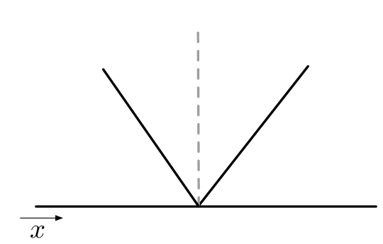
Figure 1: Structure of the Lax-Friedrichs approximate Riemann solution. The left and right states are the cell averages $u_{i},u_{j}$, while the middle state is $\bar{u}^{L}_{ij}$. The discontinuities separating these states travel at speeds $\pm\lambda_{ij}$.

2.1 Bound-preserving schemes

The first-order LLF scheme uses the cell averages $\hat{u}_{i}=u_{i}$ and $\hat{u}_{j}=u_{j}$ in (4). The numerical flux $H(u_{i},u_{j},\mathbf{n}_{ij})$ can be derived from the conservation law by assuming that the Riemann solution has the structure shown in Fig. 1, consisting of two traveling discontinuities. The conservation law holds if the intermediate state (hereafter referred to as the bar state) is given by [40]

$$\bar{u}_{ij}^{L}=\frac{u_{j}+u_{i}}{2}-\frac{{\mathbf{f}}(u_{j})-{\mathbf{f}}(u_{i})}{2\lambda_{ij}}\cdot\mathbf{n}_{ij}.$$ (5)

By the mean value theorem, the low-order (hence superscript $L$) bar states $\bar{u}_{ij}^{L}$ satisfy [32]

$$\min\{u_{i},u_{j}\}\leq\bar{u}_{ij}^{L}\leq\max\{u_{i},u_{j}\}.$$ (6)

Using (5) and the fact that $\sum_{j\in\mathcal{N}_{i}}|S_{ij}|\mathbf{f}(u_{i})\cdot{\bf n}_{ij}=0$, the first-order LLF scheme can be written as

$$|K_{i}|\frac{\mathrm{d}u_{i}}{\mathrm{d}t}=\sum_{j\in\mathcal{N}_{i}}|S_{ij}|\lambda_{ij}(\bar{u}_{ij}^{L}-u_{i})=d_{i}(\bar{u}_{i}^{L}-u_{i}),$$ (7)

where

$$\bar{u}_{i}^{L}=\frac{1}{d_{i}}\sum_{j\in\mathcal{N}_{i}}|S_{ij}|\lambda_{ij}\bar{u}_{ij}^{L},\qquad d_{i}=\sum_{j\in\mathcal{N}_{i}}|S_{ij}|\lambda_{ij}.$$ (8)

The representation of the right-hand side in terms of the jumps $\bar{u}_{ij}^{L}-u_{i}$ in the Riemann solution is known as the fluctuation form of the finite volume scheme [40]. The representation in terms of the single jump $\bar{u}_{i}^{L}-u_{i}$ reveals that an equilibrium state must be a convex combination of $\bar{u}_{ij}^{L}$.

Definition 1.

[17] We say ${\mathcal{G}}\subset{\mathbb{R}}$ is an invariant set for the initial value problem (1) if it holds that

$$u(x,0)\in{\mathcal{G}}\ \ \forall\mathbf{x}\in\bar{\Omega}\implies u(x,t)\in{\mathcal{G}}\ \ \forall\mathbf{x}\in\bar{\Omega}$$

for all $t>0$.

Definition 2.

We say a semi-discretization of (1) is bound preserving (BP) w.r.t. ${\mathcal{G}}=[u^{\min},u^{\max}]$ if

$$u_{i}(0)\in{\mathcal{G}}\ \forall i\ \implies\ u_{i}(t)\in{\mathcal{G}}\ \forall i\ \forall t>0.$$

In this case we refer to $u^{\min}$ and $u^{\max}$ as global bounds. If ${\mathcal{G}}$ is an invariant set of the initial value problem, the scheme is called invariant domain preserving (IDP) [17, 32] or (in case ${\mathcal{G}}$ is the positive orthant) positivity preserving [23, 46, 47].

Theorem 1 (Semi-discrete maximum principle).

Let

$$G=\{w\in\mathbb{R}^{N_{h}}\,:\,w_{i}\in[\alpha,\beta],\ i=1,\ldots,N_{h}\}$$

and consider the initial value problem

$$u_{i}^{\prime}(t)=a_{i}(u)(g(u)_{i}-u_{i}),\qquad u_{i}(0) =u_{i}^{0},$$ (9)

where $g$ is such that

$$u\in G\implies g(u)\in G$$ (10)

and

$$0\leq a_{i}(u)\leq C\ \ \ \forall u\in G.$$ (11)

Furthermore, assume that (9) has a unique solution for all $t>0$ for all $u^{0}\in G$. Then the solution satisfies

$$u(t)\in G\ \ \forall\ \ t\geq 0.$$ (12)

Proof.

If $a_{i}$ is independent of $i$, then this is a direct application of Nagumo’s lemma (see e.g. [4, Theorem 4.1] or [3, Theorem 3.1]. For the general case, observe that for $u\in G$ and $\epsilon<1/C$ we have

$$u_{i}(t)+\epsilon u_{i}^{\prime}(t)=(1-\epsilon a_{i}(u(t)))u_{i}+\epsilon a_{i}(u(t))g(u)_{i}\in[\alpha,\beta].$$

The result then follows from [6, Lemma 2]. ∎

The assumption of existence and uniqueness above can be avoided by invoking other assumptions such as Lipschitz continuity; see [4].

Applying the theorem above to the first-order Lax-Friedrichs scheme (7), we obtain

Corollary 1.

Let global bounds $u^{\textup{min}},u^{\textup{max}}$ be given and let

$$G=\{w\in\mathbb{R}^{N_{h}}\,:\,w\in[u^{\textup{min}},u^{\textup{max}}],\ i=1,\ldots,N_{h}\}.$$

Assume that $\lambda_{ij}$ is uniformly bounded on $G$. Then the scheme (7) is bound preserving w.r.t. $[u^{\textup{min}},u^{\textup{max}}]$.

Proof.

The first-order scheme (7) is of the form (9) with $a_{i}=d_{i}/|K_{i}|$ and $g(u)_{i}=\bar{u}_{i}$. The assumption on $\lambda_{ij}$ ensures that condition (11) holds. The validity of (10) follows from the fact that $\bar{u}_{i}=\bar{u}_{i}^{L}$ is a convex combination of the bar states $\bar{u}_{ij}^{L}$ satisfying (6). ∎

Let $\mathcal{G}=[u^{\min},u^{\max}]$ be an invariant set of problem (1). Define the range $\mathcal{G}_{i}=[u_{i}^{\min},u_{i}^{\max}]\subseteq\mathcal{G}$ of numerically admissible states using (global or local) bounds $u_{i}^{\min}$ and $u_{i}^{\max}$ such that

$$u^{\min}\leq u_{i}^{\min}\leq\min_{j\in\mathcal{V}_{i}}u_{j}\leq u_{i}\leq\max_{j\in\mathcal{V}_{i}}u_{j}\leq u_{i}^{\max}\leq u^{\max},$$ (13)

where $\mathcal{V}_{i}$ is the set containing the index $i$ and the indices of all cells that share a vertex with $K_{i}$.

Definition 3.

A BP scheme of the form (9) is called local extremum diminishing (LED) [25, 26] w.r.t. $\mathcal{G}_{i}(t)=[u_{i}^{\min}(t),u_{i}^{\min}(t)]\subset[u^{\min},u^{\max}]$ at $t\geq 0$ if

$$u_{j}\in{\mathcal{G}}_{i}\ \ \forall j\in\mathcal{V}_{i}\implies g_{i}(u)\in{\mathcal{G}}_{i}.$$

Because of (6), the first-order scheme (7) is LED w.r.t. any ${\mathcal{G}}_{i}=[u_{i}^{\min},u_{i}^{\min}]$ such that $u_{i},u_{j}\in{\mathcal{G}}_{i}$.

2.2 Bound-preserving limiters

The accuracy of the low-order approximation can be improved by using anfidiffusive fluxes $F_{ij}^{*}$ to correct the bar states $\bar{u}_{ij}^{L}$. The resulting generalization of (7) and (3) is given by

$$|K_{i}|\frac{\mathrm{d}u_{i}}{\mathrm{d}t}=\sum_{j\in\mathcal{N}_{i}}|S_{ij}|\lambda_{ij}(\bar{u}_{ij}^{*}-u_{i})=d_{i}(\bar{u}_{i}^{*}-u_{i}).$$ (14)

The flux-corrected intermediate states $\bar{u}_{ij}^{*}$ and $\bar{u}_{i}^{*}$ are defined as follows:

$$\bar{u}_{ij}^{*}=\bar{u}_{ij}^{L}+\frac{F_{ij}^{*}}{|S_{ij}|\lambda_{ij}},\qquad\bar{u}_{i}^{*}=\frac{1}{d_{i}}\sum_{j\in\mathcal{N}_{i}}|S_{ij}|\lambda_{ij}\bar{u}_{ij}^{*}=\bar{u}_{i}^{L}+\frac{1}{d_{i}}\sum_{j\in\mathcal{N}_{i}}F_{ij}^{*}.$$ (15)

For example, the high-order finite volume scheme (3) is recovered for $F_{ij}^{*}=F_{ij}$, where

$$F_{ij}=\int_{S_{ij}}[H(u_{i},u_{j},\mathbf{n}_{ij})-H(\hat{u}_{i},\hat{u}_{j},\mathbf{n}_{ij})]\,{\rm d}{\mathrm{s}}.$$ (16)

Introducing a free parameter $\gamma>0$, we limit the fluxes $F_{ij}$ in a manner which guarantees that

$$(1+\gamma)(u_{i}^{\min}-u_{i})\leq\bar{u}_{i}^{*}-u_{i}\leq(1+\gamma)(u_{i}^{\max}-u_{i}).$$ (17)

The resulting scheme is BP for any $\gamma>0$. Indeed, (14) can be written in the form (9) with

$$a_{i}=(1+\gamma)\frac{d_{i}}{|K_{i}|},\qquad g_{i}(u)=u_{i}+\frac{\bar{u}_{i}^{*}-u_{i}}{1+\gamma}\in[u_{i}^{\min},u_{i}^{\max}].$$ (18)

Let us now discuss the way to calculate the limited counterparts $F_{ij}^{*}$ of the fluxes $F_{ij}$. Recalling the definition (15) of $\bar{u}_{i}^{*}$, we find that the inequality constraints (17) hold if and only if

$$Q_{i}^{-}\leq\sum_{j\in\mathcal{N}_{i}}F_{ij}^{*}\leq Q_{i}^{+},$$ (19)

where

$$Q_{i}^{-}=d_{i}[(u_{i}^{\min}-\bar{u}_{i}^{L})+\gamma(u_{i}^{\min}-u_{i})],\quad Q_{i}^{+}=d_{i}[(u_{i}^{\max}-\bar{u}_{i}^{L})+\gamma(u_{i}^{\max}-u_{i})].$$ (20)

The use of $\gamma>0$ in (20) relaxes the bounds $Q_{i}^{\pm}$ in a way that makes the flux constraints (19) less restrictive. As a result, higher accuracy can be achieved using larger values of $\gamma$. However, the CFL condition for explicit schemes becomes more restrictive, as we show in Section 3 below.

By definition of $d_{i}$ and $\bar{u}_{i}^{L}$, the bounds $Q_{i}^{\pm}$ of the flux constraints (19) can be decomposed into

$$Q_{ij}^{-}=|S_{ij}|\lambda_{ij}[(u_{i}^{\min}-\bar{u}_{ij}^{L})+\gamma(u_{i}^{\min}-u_{i})],\quad Q_{ij}^{+}=|S_{ij}|\lambda_{ij}[(u_{i}^{\max}-\bar{u}_{ij}^{L})+\gamma(u_{i}^{\max}-u_{i})].$$ (21)

Localized flux limiting algorithms [9, 15, 32, 42] use such decompositions to replace inequality constraints for sums of fluxes by sufficient conditions that make it possible to constrain each flux independently. The local monolithic convex (LMC) limiting algorithm proposed in [32] yields

$$F_{ij}^{*}=\begin{cases}\min\,\{Q_{ij}^{+},F_{ij},-Q_{ji}^{-}\}&\mbox{if}\ F_{ij}>0,\\[7.11317pt] \max\,\{Q_{ij}^{-},F_{ij},-Q_{ji}^{+}\}&\mbox{otherwise},\end{cases}$$ (22)

where $F_{ij}$ is the antidiffusive flux defined by (16). The LMC limiter is designed to guarantee that

$$Q_{ij}^{-}\leq F_{ij}^{*}\leq Q_{ij}^{+},\qquad F_{ji}^{*}=-F_{ij}^{*},\qquad Q_{ji}^{-}\leq F_{ji}^{*}\leq Q_{ji}^{-}.$$ (23)

Hence, the flux-corrected scheme is conservative and satisfies conditions (19) for $i=1,\ldots,N_{h}$.

To avoid a potential loss of accuracy due to localization of the flux constraints, we introduce a global monolithic convex (GMC) limiter that enforces (19) using the following algorithm:

1. Calculate the sums of positive and negative antidiffusive fluxes

   $$P_{i}^{+}=\sum_{j\in\mathcal{N}_{i}}\max\{0,F_{ij}\},\qquad P_{i}^{-}=\sum_{j\in\mathcal{N}_{i}}\min\{0,F_{ij}\}.$$ (24)

2. Use the sums $P_{i}^{\pm}$ and the bounds $Q_{i}^{\pm}$ defined by (20) to calculate

   $$R_{i}^{+}=\min\left\{1,\frac{Q_{i}^{+}}{P_{i}^{+}}\right\},\qquad R_{i}^{-}=\min\left\{1,\frac{Q_{i}^{-}}{P_{i}^{-}}\right\}.$$ (25)

3. Calculate the limited antidiffusive fluxes $F_{ij}^{*}=\alpha_{ij}F_{ij}$, where

   $$\alpha_{ij}=\begin{cases}\min\{R^{+}_{i},R^{-}_{j}\}&\mbox{if}\ F_{ij}>0,\\ 1&\mbox{if}\ F_{ij}=0,\\ \min\{R^{-}_{i},R^{+}_{j}\}&\mbox{if}\ F_{ij}<0.\end{cases}$$ (26)

This limiting strategy is based on Zalesak’s FCT algorithm [45] but the GMC bounds (20) are independent of the time step, and the validity of a discrete maximum principle is guaranteed for any strong stability preserving (SSP) Runge-Kutta time integrator [13, 14]. In Section 3, we verify this claim for a single forward Euler step and discuss flux limiting for general Runge-Kutta stages.

3 Flux limiting for Runge-Kutta methods

Given a BP space discretization of the form (9) and a time step $\Delta t>0$, the first-order accurate forward Euler (FE) method advances the cell averages $u_{i},\ i=1,\ldots,N_{h}$ in time as follows:

$$u^{n+1}=u_{i}^{n}+\nu_{i}(\bar{u}_{i}^{n}-u_{i}^{n})=(1-\nu_{i})u_{i}^{n}+\nu_{i}\bar{u}_{i}^{n},$$ (27)

where $\nu_{i}=\Delta ta_{i}>0$ is a generalized ‘CFL’ number. If $\nu_{i}\leq 1$ then $u_{i}^{n+1}$ is a convex combination of $u_{i}^{n}$ and $\bar{u}_{i}^{n}$. It follows that $u_{i}^{n+1}\in[u_{i}^{\min},u_{i}^{\max}]$ if $u_{i}^{n},\bar{u}_{i}^{n}\in[u_{i}^{\min},u_{i}^{\max}]$. In view of (18), the fully discrete version of the semi-discrete scheme (14) equipped with the LMC or GMC flux limiter is BP if

$$(1+\gamma)\frac{\Delta td_{i}}{|K_{i}|}\leq 1.$$ (28)

The low-order LLF scheme (7) and Zalesak’s FCT method are BP for time steps satisfying (28) with $\gamma=0$. The FCT fluxes $F_{ij}^{*}$ are calculated using algorithm (24)–(26) with global bounds

$$Q_{i}^{-}=\frac{|K_{i}|}{\Delta t}(u_{i}^{\min}-u_{i}^{\rm FE}),\qquad Q_{i}^{+}=\frac{|K_{i}|}{\Delta t}(u_{i}^{\max}-u_{i}^{\rm FE})$$ (29)

depending on $u_{i}^{\rm FE}=u_{i}^{n}+\frac{\Delta t}{|K_{i}|}d_{i}(\bar{u}_{i}^{L}-u_{i}^{n})$. A localized version of FCT is defined by (22) with [34]

$$Q_{ij}^{-}=\frac{|K_{i}|\,|S_{ij}|}{\Delta t|\partial K_{i}|}(u_{i}^{\min}-u_{i}^{\rm FE}),\qquad Q_{ij}^{+}=\frac{|K_{i}|\,|S_{ij}|}{\Delta t|\partial K_{i}|}(u_{i}^{\max}-u_{i}^{\rm FE}).$$ (30)

Flux limiting techniques of this kind were considered, e.g., in [15, 32, 34]. The main advantage of localized convex limiting lies in its applicability to systems. Since the main focus of the present paper is on scalar conservation laws, we restrict further discussion to global MC and FCT limiters.

Remark 4.

Since the FCT bounds (29) and (30) depend on the time step and on the low-order predictor $u_{i}^{\rm FE}$, the resulting nonlinear schemes have no semi-discrete or steady-state counterparts.

3.1 High-order Runge-Kutta methods

Let us rewrite (14) as

$$|K_{i}|\frac{\mathrm{d}u_{i}}{\mathrm{d}t}=-\sum_{j\in\mathcal{N}_{i}}|S_{ij}|H_{ij}^{*}(\hat{u}),\qquad H_{ij}^{*}\left(\hat{u}\right)=H(u_{i},u_{j},\mathbf{n}_{ij})-\frac{F_{ij}^{*}(\hat{u})}{|S_{ij}|},$$ (31)

where $\hat{u}$ is a high-order piecewise-polynomial reconstruction from the cell averages $u_{1},\ldots,u_{N_{h}}$.

We now discretize (14) in time using an explicit $M$-stage Runge-Kutta (RK) method with coefficients denoted by the vectors $c,b$ and matrix $A$. The RK stage approximations $y_{i}^{(m)}\approx u_{i}(t^{n}+c_{m}\Delta t)$ to the cell averages are given by

$$y_{i}^{(1)} =u_{i}^{n},$$ (32a)

$$y_{i}^{(m)} =u_{i}^{n}-\frac{\Delta t}{|K_{i}|}\sum_{j\in\mathcal{N}_{i}}|S_{ij}|\sum_{s=1}^{m-1}a_{ms}H_{ij}^{*}\left(\hat{y}^{(s)}\right),\qquad m=2,\ldots,M.$$ (32b)

The RK solution $u_{i}^{\rm RK}\approx u_{i}(t^{n}+\Delta t)$ is defined as

$$u_{i}^{\rm RK}=u_{i}^{n}-\frac{\Delta t}{|K_{i}|}\sum_{j\in\mathcal{N}_{i}}|S_{ij}|H_{ij}^{\rm RK},\qquad H_{ij}^{\rm RK}=\sum_{m=1}^{M}b_{m}H_{ij}^{*}\left(\hat{y}^{(m)}\right).$$ (33)

Note that the intermediate cell averages $y_{i}^{(2)},\ldots,y_{i}^{(M)}$ are generally not BP even for the low-order LLF scheme, i.e., in the case $\hat{y}_{i}^{(m)}\equiv y_{i}^{(m)}$. However, if a RK stage can be written as a convex combination of forward Euler steps (27), then it inherits their BP properties. It is therefore useful to distinguish between three classes of RK methods. To facilitate their definition, let

$$X(\mu)=\left(I+\mu A\right)^{-1},$$ (34)

where $\mu>0$ is a stability parameter and $I$ is the identity matrix. Furthermore, let $e$ denote the vector of length $M$ with all entries equal to unity.

3.1.1 Strong stability preserving (SSP) methods

An explicit Runge-Kutta method is strong stability preserving (SSP) if it is possible to write the stage approximations $y_{i}^{(2)},\ldots,y_{i}^{(M)}$ and the final solutions $u_{i}^{\rm RK}$ as convex combinations of forward Euler predictors $u_{i}^{(1)},\ldots,u_{i}^{(\tilde{M})}$. For $\tilde{M}\in\{1,2,3,5\}$, the optimal explicit SSP-RK methods use

$$u_{i}^{(1)} =u^{n},$$ (35a)

$$u_{i}^{(m)} =u_{i}^{(m-1)}-\frac{\Delta t}{|K_{i}|}\sum_{j\in\mathcal{N}_{i}}|S_{ij}|H_{ij}^{*}(u_{i}^{(m-1)}),\qquad m=2,\ldots,\tilde{M}.$$ (35b)

If the space discretization (31) is BP, then so is the resulting full discretization. The maximum order of such SSP-RK time integrators is 4 in the explicit case and 6 in the implicit case [13]. For comparison with the next class of methods, we note that SSP methods satisfy the entrywise inequalities

$$AX(\mu)\geq 0,\ \ \ \ AX(\mu)e\leq e,$$ (36)

as well as

$$b^{T}X(\mu)\geq 0,\ \ \ \ b^{T}X(\mu)e\leq 1,$$ (37)

with an SSP coefficient $\mu>0$ such that the fully discrete scheme is BP for $\Delta t\leq\mu\Delta t^{\rm FE}$ if the forward Euler method is BP for $\Delta t\leq\Delta t^{\rm FE}$; see [13] for details.

3.1.2 Internal SSP methods

A larger class of RK methods satisfy (36) for some $\mu>0$ but may violate (37). That is, all intermediate approximations $u_{i}^{(1)},\ldots,u_{i}^{(\tilde{M})}$ are BP for $\Delta t\leq\mu\Delta t^{\rm FE}$ but the weights of the final linear combination $u_{i}^{\rm RK}=\sum_{m=1}^{\tilde{M}}\beta_{m}u_{i}^{(m)}$ are not necessarily positive. The family of such internal SSP methods includes all SSP schemes, but also many other methods, such as extrapolation methods based on the explicit Euler method (see, e.g., [18, Section II.9]), whose implementation details are presented in Algorithm 1 and Table 1. We use these methods in some numerical experiments in Section 5. They have an advantage over SSP methods in that they can be constructed to have any desired order of accuracy. Since the final stage of these methods is not BP, we constrain it using a flux limiter as described in Section 3.2.

3.1.3 General RK methods

A high-order Runge-Kutta method with Butcher stages of the form (32a)–(32b) and (33) is generally not BP. Hence, flux limiting may be required in intermediate stages and/or in the final stage.

Algorithm 1 Explicit Euler extrapolation (Ex-Euler) for $\frac{\mathrm{d}u}{\mathrm{d}t}=F(u)$

$y^{(1)}:=u^{n}$

$m:=1$

for $s=1\to S$ do

     $m:=m+1$

     $y^{(m)}:=u^{n}+\frac{\Delta t}{s}F(u^{n})$

     for $k=2\to s-1$ do

         $m:=m+1$

         $y^{(m)}:=y^{(m-1)}+\frac{\Delta t}{s}F(y^{(m-1)})$

     end for

end for

$M:=m$

$u^{n+1}:=u^{n}+\Delta t\sum_{m=1}^{M}b_{m}F(y^{(m)})$

Order	Weights $[b_{1},\ldots,b_{M}]$
2	$[0,1]$
3	$[0,-2,3/2,3/2]$
4	$[0,2,-9/2,-9/2,8/3,8/3,8/3]$
5	$[0,-4/3,27/4,27/4,-32/3,-32/3,-32/3,125/24,125/24,125/24,125/24]$

Table 1: Weights for extrapolation methods, to be used in Algorithm 1.

3.2 Flux limiting for the final RK stage

If the employed time-stepping method is not SSP and/or the space discretization (31) uses the unlimited antidiffusive fluxes $F_{ij}^{*}=F_{ij}$, the bound-preserving low-order FE-LLF scheme

$$u_{i}^{\rm FE}=u_{i}^{n}-\frac{\Delta t}{|K_{i}|}\sum_{j\in\mathcal{N}_{i}}|S_{ij}|H_{ij}^{\rm FE},\qquad H_{ij}^{\rm FE}=H(u_{i}^{n},u_{j}^{n},\mathbf{n}_{ij})$$ (38)

can be combined with the final stage (33) of the high-order RK-LLF method

$$u_{i}^{\rm RK}=u_{i}^{n}-\frac{\Delta t}{|K_{i}|}\sum_{j\in\mathcal{N}_{i}}|S_{ij}|H_{ij}^{\rm RK}=u_{i}^{\rm FE}+\frac{\Delta t}{|K_{i}|}\sum_{j\in\mathcal{N}_{i}}F_{ij}^{\rm RK},\qquad F_{ij}^{\rm RK}=|S_{ij}|(H_{ij}^{\rm FE}-H_{ij}^{\rm RK})$$ (39)

to produce a nonlinear flux-limited approximation of the form

$$u_{i}^{n+1}=u_{i}^{n}-\frac{\Delta t}{|K_{i}|}\sum_{j\in\mathcal{N}_{i}}|S_{ij}|\left[\alpha_{ij}H_{ij}^{\rm RK}+(1-\alpha_{ij})H_{ij}^{\rm FE}\right]=u_{i}^{\rm FE}+\frac{\Delta t}{|K_{i}|}\sum_{j\in\mathcal{N}_{i}}\alpha_{ij}F_{ij}^{\rm RK}.$$ (40)

This fully discrete scheme reduces to (38) for $\alpha_{ij}=0$ and to (33) for $\alpha_{ij}=1$. It is BP w.r.t. the admissible set $\mathcal{G}_{i}=[u_{i}^{\min},u_{i}^{\max}]$ if the definition of the correction factors $\alpha_{ij}$ guarantees that

$$u_{i}^{\min}\leq u_{i}^{n+1}\leq u_{i}^{\max}.$$ (41)

Zalesak’s FCT method [45] preserves the BP property of $u_{i}^{\rm FE}$ using algorithm (24)–(26) to calculate correction factors $\alpha_{ij}$ such that the limited fluxes $F_{ij}^{*}=\alpha_{ij}F_{ij}^{\rm RK}$ satisfy

$$Q_{i}^{-}=\frac{|K_{i}|}{\Delta t}\left(u_{i}^{\min}-u_{i}^{\rm FE}\right)\leq\sum_{j\in\mathcal{N}_{i}}F_{ij}^{*}\leq\frac{|K_{i}|}{\Delta t}\left(u_{i}^{\max}-u_{i}^{\rm FE}\right)=Q_{i}^{+}.$$ (42)

We remark that the temporal accuracy of classical FCT schemes is restricted to second order. To our knowledge, the first combination of FCT with high-order RK methods was considered in [42].

As an alternative to FCT, we propose a flux limiter that calculates $F_{ij}^{*}$ using the GMC bounds (20) in algorithm (24)–(26). Invoking (18), the flux-corrected scheme can again be written as

$$u_{i}^{n+1}=u_{i}^{n}+(1+\gamma)\frac{\Delta td_{i}}{|K_{i}|}\left(\bar{u}_{i}^{n}-u_{i}^{n}\right),$$

where $\bar{u}_{i}^{n}\in[u_{i}^{\min},u_{i}^{\max}]$. This proves that the fully discrete scheme is BP for time steps satisfying (28).

Remark 5.

Update (40) is mass conservative in the sense that $\sum_{i=1}^{N_{h}}|K_{i}|u_{i}^{n+1}=\sum_{i=1}^{N_{h}}|K_{i}|u_{i}^{n}$ because the correction factors satisfy the symmetry condition $\alpha_{ij}=\alpha_{ji}$ and the fluxes sum to zero.

Remark 6.

Unlike FCT-like predictor-corrector approaches, the GMC limiter produces correction factors $\alpha_{ij}$ that do not depend on $\Delta t$. Consequently, this flux limiting strategy leads to well-defined nonlinear discrete problems and does not inhibit convergence to steady-state solutions.

3.3 Flux limiting for intermediate RK stages

If the BP property needs to be enforced not only at the final stage (33) but also at intermediate stages (32b) of the Runge-Kutta method, flux-corrected approximations of the form

$$y_{i}^{*,(m)}=u_{i}^{n}-\frac{\Delta t}{|K_{i}|}\sum_{j\in\mathcal{N}_{i}}\left[c_{m}|S_{ij}|H_{ij}^{\rm FE}-F_{ij}^{*,(m)}\right]=y_{i}^{{\rm FE},(m)}+\frac{\Delta t}{|K_{i}|}\sum_{j\in\mathcal{N}_{i}}F_{ij}^{*,(m)}$$ (43)

can be calculated using

$$y_{i}^{{\rm FE},(m)}=u_{i}^{n}-\frac{c_{m}\Delta t}{|K_{i}|}\sum_{j\in\mathcal{N}_{i}}|S_{ij}|H_{ij}^{\rm FE},\qquad F_{ij}^{*,(m)}=\alpha_{ij}^{(m)}F_{ij}^{(m)},$$ (44)

where

$$F_{ij}^{(m)}=c_{m}|S_{ij}|H_{ij}^{\rm FE}-\sum_{s=1}^{m-1}a_{ms}\int_{S_{ij}}H_{ij}\big{(}\hat{y}^{(s)}\big{)}\,{\rm d}{\mathrm{s}},$$ (45)

is the antidiffusive flux. Here we used the simplified notation

$$H_{ij}(z):=H(z_{i}({\bf x}),z_{j}({\bf x}),\mathbf{n}_{ij}).$$ (46)

The correction factors $\alpha_{ij}^{(m)}$ can be calculated as in Section 3.2. In the GMC version of the flux limiting procedure, the bounds $Q_{i}^{\pm}$ should be multiplied by $c_{m}$.

3.4 Slope limiting for high-order reconstructions

Stagewise limiting guarantees the BP property of the cell averages $y_{i}^{(s)}$. If the calculation of $H_{ij}\left(\hat{y}^{(s)}\right)$ requires the BP property of the high-order reconstructions $\hat{y}_{i}^{(s)}:K_{i}\to\mathbb{R}$, it can be enforced using slope limiting to blend a reconstructed polynomial $\hat{y}_{i}^{(s)}$ and a BP cell average as follows:

• If an intermediate cell average $y_{i}$ is BP w.r.t. $[u_{i}^{\min},u_{i}^{\max}]$, then there exists $\theta_{i}\in[0,1]$ such that

  $$\hat{y}_{i}^{*}(\mathbf{x}_{p}):=y_{i}+\theta_{i}\left(\hat{y}_{i}(\mathbf{x}_{p})-y_{i}\right)\in[u_{i}^{\min},u_{i}^{\max}]$$ (47)

  at each quadrature point $\mathbf{x}_{p}\in\partial K_{i}$ at which the value of $\hat{y}_{i}^{*}(\mathbf{x}_{p})$ is required for calculation of $H_{ij}$. Adapting the Barth-Jespersen formula [2] to this setting, we define the correction factor

  $$\theta_{i}=\min_{p}\left\{\begin{array}[]{ll}\min\left\{1,\frac{u^{\max}_{i}-y_{i}}{\hat{y}_{i}(\mathbf{x}_{p})-y_{i}}\right\}&\mbox{if}\ \ \hat{y}_{i}(\mathbf{x}_{p})>u^{\max}_{i},\\ 1&\mbox{if}\ \ \hat{y}_{i}(\mathbf{x}_{p})\in[u^{\min}_{i},u^{\max}_{i}],\\ \min\left\{1,\frac{u^{\min}_{i}-y_{i}}{\hat{y}_{i}(\mathbf{x}_{p})-y_{i}}\right\}&\mbox{if}\ \ \hat{y}_{i}(\mathbf{x}_{p})<u^{\min}_{i}.\end{array}\right.$$ (48)

  We remark that slope limiters of this kind were used, e.g., by Zhang and Shu [46, 47] in the context of positivity-preserving WENO-DG schemes combined with SSP-RK time discretizations.

• If the intermediate cell averages are not BP because the RK method does not satisfy (36) or the flux limiter for $F_{ij}^{(m)}$ is deactivated, limited reconstructions of the form

  $$\hat{y}_{i}^{*}(\mathbf{x}_{p}):=u_{i}^{n}+\theta_{i}(\hat{y}_{i}(\mathbf{x}_{p})-u_{i}^{n})\in[u_{i}^{\min},u_{i}^{\max}]$$ (49)

  may be employed. The conservation properties of the limited scheme are not affected by using a convex combination of $\hat{y}_{i}$ and $u_{i}^{n}$ for calculation of the high-order LLF fluxes $H_{ij}(\hat{y}_{i}^{*})$.

4 Case study: flux-limited WENO-RK schemes

As mentioned in the introduction, the presented flux limiters can be applied to different kinds of high-order discretizations in space and time. In the numerical experiments of Section 5, we use a fifth-order WENO spatial discretization combined with explicit high-order Runge-Kutta methods. The corresponding sequence of solution updates is defined by the Butcher tableau

(56)

To illustrate the use of limiting techniques for antidiffusive fluxes depending on time and/or space discretizations, we now detail specific combinations of high-order RK methods with GMC-type flux limiters. A numerical study of the following RK methods is performed in Section 5:

• SSP54: a fourth-order strong stability preserving method.

• ExE-RK5: a fifth-order extrapolated Euler Runge-Kutta method.

• RK76: a sixth-order Runge-Kutta method.

The details of these time integration methods can be found in A. The algorithms presented in B define WENO-GMC discretizations for uniform grids in 1D. Since SSP time discretizations preserve the BP properties of flux-corrected semi-discrete schemes, we equip the SSP54 method with the spatial GMC limiter derived in Section 2.2. For extrapolation methods, the application of this limiter is sufficient to guarantee that intermediate solutions are BP but the final stage needs to be constrained using (40). For general RK methods, the space-time limiting techniques of Sections 3.2 and 3.3 can be used to enforce the BP property. In this context, a flux limiter can be invoked in each stage or only in the final stage (allowing bound-violating approximations in the intermediate stages). We therefore test the following limiting strategies for the RK methods under investigation:

• SSP54-GMC: SSP54 with GMC space limiting for $F_{ij}^{(m)}$ in each intermediate stage.

• ExE-RK5-GMC: ExE-RK5 with GMC space limiting for $F_{ij}^{(m)}$ in each intermediate stage and GMC space-time limiting for $F_{ij}^{\rm RK}$ in the final stage.

• RK76-GMC: RK76 with GMC space-time limiting for $F_{ij}^{\rm RK}$ only in the final stage.

• Sw-RK76-GMC: RK76 with GMC space-time limiting for $F_{ij}^{(m)}$ in each intermediate stage and for $F_{ij}^{\rm RK}$ in the final stage.

The SSP54-GMC and RK76-GMC methods are tested in all numerical experiments of Section 5. To demonstrate that stagewise BP limiting does not degrade the high-order accuracy of the baseline scheme, at least if the bounds are global, we include the results of ExE-RK5-GMC and Sw-RK76-GMC convergence studies for test problems with smooth exact solutions. In the rest of the numerical experiments, the stagewise BP schemes perform similarly to SSP54-GMC and RK76-GMC. Therefore, no further ExE-RK5-GMC and Sw-RK76-GMC results are reported in Section 5.

4.1 Summary of the fully discrete BP schemes

For the reader’s convenience, we now summarize the main steps of the fully discrete BP algorithms.

4.1.1 Implementation of SSP54-GMC

The formulas for the stage approximations $y_{i}^{(1)},\ldots,y_{i}^{(5)}$ are presented in A.1. The final stage result is given by $u_{i}^{n+1}=y_{i}^{(5)}$. For $k=1,\ldots,4$, we need to evaluate the time derivatives

$$F_{i}(y^{(k)}):=\frac{1}{|K_{i}|}\sum_{j\in\mathcal{N}_{i}}|S_{ij}|\lambda_{ij}\big{(}y^{(k)}\big{)}\big{(}\bar{u}_{ij}^{*}\big{(}y^{(k)}\big{)}-y_{i}^{(k)}\big{)},$$ (57)

where $\lambda_{ij}$ is an upper bound for the wave speed of the Riemann problem associated with face $S_{ij}$. In Section 5, we specify the values of $\lambda_{ij}$ that we use for the different numerical experiments. For $u\in\{y_{i}^{(1)},\ldots,y_{i}^{(5)}\}$, we calculate the bar states $\bar{u}_{ij}^{*}(u)$ as follows:

1. Compute the low-order bar states $\bar{u}_{ij}^{L}$ using (5).

2. Compute the antidiffusive fluxes $F_{ij}$ using (16).

3. Compute the GMC bounds $Q_{i}^{\pm}$ defined by (20).

4. Compute the correction factors $\alpha_{ij}$ using (24)-(26).

5. Compute the limited antidiffusive fluxes $F_{ij}^{*}=\alpha_{ij}F_{ij}$.

6. Compute the flux-corrected bar states $\bar{u}_{ij}^{*}$ using (15).

4.1.2 Implementation of ExE-RK5-GMC

The ExE-RK5 method that we use is defined in A.2. The BP stage approximations $y_{i}^{(1)},\ldots,y_{i}^{(11)}$ are calculated as in Section 4.1.1. In the final stage, we update $u=u^{n}$ as follows:

1. Compute the low-order bar states $\bar{u}_{ij}^{L}$ using (5).

2. Compute the high-order fluxes $H_{ij}^{\rm RK}$ using (33).

3. Compute the low-order fluxes $H_{ij}^{\rm FE}=H(u_{i}^{n},u_{j}^{n},\mathbf{n}_{ij})$.

4. Compute the antidiffusive fluxes $F_{ij}^{\rm RK}=|S_{ij}|(H_{ij}^{\rm FE}-H_{ij}^{\rm RK})$.

5. Compute the low-order predictor $u_{i}^{\rm FE}$ using (38).

6. Compute the GMC bounds $Q_{i}^{\pm}$ defined by (20).

7. Compute the correction factors $\alpha_{ij}$ using (24)-(26).

8. Use $F_{ij}^{*}=\alpha_{ij}F_{ij}^{\rm RK}$ to compute $u_{i}^{n+1}$ defined by (40).

4.1.3 Implementation of RK76-GMC

The Butcher tableau of the RK76 method is presented in A.3. The stage approximations $y_{i}^{(1)},\ldots,y_{i}^{(7)}$ are calculated using (32) without applying any flux limiter. The final RK update is constrained using the GMC space-time limiter, i.e., the algorithm presented in Section 4.1.2.

4.1.4 Implementation of Sw-RK76-GMC

To constrain the intermediate Butcher stages of the RK76 method, we proceed as follows:

1. Compute the low-order predictor $y_{i}^{{\rm FE},(m)}$ using (44).

2. Compute the antidiffusive flux $F_{ij}^{(m)}$ using (45).

3. Compute the GMC bounds $Q_{i}^{\pm}$ defined by (20).

4. Compute the correction factors $\alpha_{ij}^{(m)}$ using (24)-(26).

5. Use $F_{ij}^{*,(m)}=\alpha_{ij}^{(m)}F_{ij}^{(m)}$ to compute $y_{i}^{*,(m)}$ defined by (43).

To guarantee that the final RK update is BP, we again use the algorithm presented in Section 4.1.2.

5 Numerical examples

In this section, we perform a series of numerical experiments to study the properties of the methods selected in Section 4. We begin with an accuracy test for WENO and WENO-GMC space discretizations. Then we test the flux-limited WENO-RK methods for time-dependent problems.

Unless mentioned otherwise, we use a fifth-order WENO [43] spatial discretization on a uniform mesh of $N_{h}$ one-dimensional cells $K_{i}=[x_{i-1/2},x_{i+1/2}]$ with $|K_{i}|=\Delta x$. For time-dependent problems, the default choice of the time step is $\Delta t=0.4\Delta x/(1+\gamma)$, where $\gamma\geq 0$ is the parameter of the limiting constraints (17). In all experiments, we enforce the global bounds of the initial data $u(x,0)$, i.e., use

$$u_{i}^{\min} =u^{\min}:=\min_{x}u(x,0),$$

$$u_{i}^{\max} =u^{\max}:=\max_{x}u(x,0)$$

for $i=1,\dots,N_{h}$. To quantify the magnitude of undershoots and overshoots (if any), we report

$$\delta=\min\{\delta^{-},\delta^{+}\},$$ (58)

where

$$\delta^{-}=\min_{t}~{}\min_{i=1,\dots,N_{h}}~{}u_{i}(t)-u^{\min},\qquad\delta^{+}=\min_{t}~{}\min_{i=1,\dots,N_{h}}~{}u^{\max}-u_{i}(t).$$

Note that $\delta\geq 0$ for any BP numerical solution. In practice, the low-order and flux-limited methods are positivity preserving to machine precision. Therefore, a numerical value of $\delta$ may be a small negative number. Since conservation laws are also satisfied to machine precision, it is acceptable to simply clip the solution. If the exact solution is available, we calculate the discrete $L_{1}$ error

$$E_{1}(t) =\Delta x\sum_{i=1}^{N_{h}}|\tilde{u}_{i}(t)-u^{\text{exact}}(x_{i},t)|$$

and the corresponding Experimental Order of Convergence (EOC) using the following fifth-order polynomial reconstruction of the numerical solution at the center $x_{i}$ of the cell:

$$\tilde{u}_{i}=\frac{1}{1920}\left(9u_{i-2}-116u_{i-1}+2134u_{i}-116u_{i+1}+9u_{i+2}\right).$$

5.1 Convergence of a WENO-GMC semi-discretization

In this section, we test the convergence properties of the spatial semi-discretization using the GMC limiters from Section 2. To this end, we consider the one-dimensional conservation law

$$\frac{\partial u}{\partial t}+\frac{\partial f(u)}{\partial x}=0\quad\mbox{ in }\quad\Omega=(0,1),$$ (59)

where $f(u)$ is the flux function. The time derivative of the exact cell average is given by

$$\frac{\mathrm{d}u_{i}}{\mathrm{d}t}=-\frac{1}{\Delta x}\int_{x_{i-1/2}}^{x_{i+1/2}}\frac{\partial f(u)}{\partial x}\mathrm{d}x=-\frac{f(u(x_{i+1/2}))-f(u(x_{i-1/2}))}{\Delta x}.$$ (60)

We discretize (59) in space using a fifth-order WENO scheme which approximates (60) by

$$\frac{\mathrm{d}u_{i}^{\rm WENO}}{\mathrm{d}t}=-\frac{H\left(\hat{u}_{i}^{+},\hat{u}_{i+1}^{-},1\right)-H\left(\hat{u}_{i-1}^{+},\hat{u}_{i}^{-},1\right)}{\Delta x}.$$ (61)

The Lax-Friedrichs flux $H(\cdot,\cdot,\cdot)$ is defined using $\lambda_{i+1/2}=\max\{u_{i},u_{i+1},\hat{u}_{i}^{+},\hat{u}_{i+1}^{-}\}$ in this test. The interface values $\hat{u}_{i}^{-}=\hat{u}_{i}(x_{i-1/2})$ and $\hat{u}_{i}^{+}=\hat{u}_{i}(x_{i+1/2})$ are determined by evaluating the WENO polynomial reconstruction $\hat{u}_{i}\in\mathbb{P}_{5}(K_{i})$ at the cell interfaces $x_{i\pm 1/2}$.

Applying the GMC flux limiter to (61), we obtain the WENO-GMC semi-discretization

$$\frac{\mathrm{d}u_{i}^{\rm GMC}}{\mathrm{d}t}=(\lambda_{i+1/2}+\lambda_{i-1/2})\frac{\bar{u}_{i}^{*}-u_{i}}{\Delta x}.$$ (62)

To assess its spatial accuracy, we consider $u(x)=\exp\left(-100(x-0.5)^{2}\right)$ and the nonlinear flux function $f(u)=u^{2}/2$. In Table 2, we report the discrete $L^{1}$ errors

$$E_{1}^{{\rm WENO}} =\Delta x\sum_{i=1}^{N_{h}}\left|\frac{\mathrm{d}u_{i}}{\mathrm{d}t}-\frac{\mathrm{d}u_{i}^{{\rm WENO}}}{\mathrm{d}t}\right|,$$

$$E_{1}^{{\rm GMC}} =\Delta x\sum_{i=1}^{N_{h}}\left|\frac{\mathrm{d}u_{i}}{\mathrm{d}t}-\frac{\mathrm{d}u_{i}^{{\rm GMC}}}{\mathrm{d}t}\right|,$$

as well as the EOCs of the WENO and WENO-GMC semi-discretizations. We consider multiple values of the GMC parameter $\gamma\geq 0$ and achieve optimal convergence rates with $\gamma\geq 0.5$.

$N_{h}$	$E_{1}^{{\rm WENO}}$	EOC	$E_{1}^{{\rm GMC}}$, $\gamma=0$	EOC	$E_{1}^{{\rm GMC}}$, $\gamma=0.5$	EOC	$E_{1}^{{\rm GMC}}$, $\gamma=1$	EOC
25	1.35e-03	–	1.35e-03	–	1.35e-03	–	1.35e-03	–
50	6.82e-05	4.30	5.12e-04	1.40	6.82e-05	4.30	6.82e-05	4.30
100	1.04e-06	6.04	6.60e-05	2.95	1.04e-06	6.04	1.04e-06	6.04
200	1.53e-08	6.08	8.30e-06	2.99	1.53e-08	6.08	1.53e-08	6.08
400	2.29e-10	6.06	1.04e-06	3.00	2.29e-10	6.06	2.29e-10	6.06
800	3.48e-12	6.04	1.30e-07	3.00	3.48e-12	6.04	3.48e-12	6.04
1600	5.36e-14	6.02	1.63e-08	3.00	5.36e-14	6.02	5.36e-14	6.02

Table 2: Grid convergence study for the 5th-order WENO and WENO-GMC discretizations of $\frac{\partial}{\partial x}(u^{2}/2)$.

5.2 Linear advection

The first test problem for our numerical study of the flux-limited space-time discretizations defined in Section 4 is the one-dimensional linear advection equation

$$\frac{\partial u}{\partial t}+a\frac{\partial u}{\partial x}=0\quad\mbox{ in }\quad\Omega=(0,1)$$ (63)

with constant velocity $a=1$. The initial condition is given by the smooth function

$$u(x,0)=\exp(-100(x-0.5)^{2}).$$ (64)

We solve (63) up to the final time $t=1$ using $\lambda_{i+1/2}=1$ for all $i$. The results of a grid convergence study for SSP54-GMC, ExE-RK5-GMC, RK76-GMC, Sw-RK76-GMC, and the underlying WENO-RK discretizations are shown in Table 3. The negative values of $\delta$ indicate that the high-order baseline schemes may, indeed, produce undershoots or overshoots on coarse meshes.

In this test, all GMC-constrained schemes deliver optimal convergence rates for $\gamma=1$. The only scheme that preserves the full accuracy for $\gamma=0$ is RK76-GMC, the method which performs flux limiting just once per time step. We remark that even this least dissipative method requires the use of $\gamma>0$ to achieve optimal EOCs for other test problems that we consider below.

	baseline			GMC, $\gamma=0$			GMC, $\gamma=1$
$N_{h}$	$E_{1}$	EOC	$\delta$	$E_{1}$	EOC	$\delta$	$E_{1}$	EOC	$\delta$
25	2.43e-02	–	-2.00e-05	2.43e-02	–	1.28e-10	2.43e-02	–	7.58e-11
50	2.30e-03	3.40	-3.26e-08	2.41e-03	3.34	2.03e-11	2.29e-03	3.40	4.95e-12
100	1.22e-04	4.24	-6.45e-11	1.37e-04	4.13	5.64e-12	1.22e-04	4.23	1.07e-12
200	4.22e-06	4.85	1.65e-11	1.35e-05	3.34	1.65e-11	4.22e-06	4.85	1.65e-11
400	1.35e-07	4.97	1.51e-11	1.89e-06	2.84	1.51e-11	1.35e-07	4.97	1.51e-11
800	4.24e-09	4.99	1.45e-11	2.89e-07	2.71	1.45e-11	4.24e-09	4.99	1.45e-11
1600	2.17e-10	4.29	1.42e-11	4.48e-08	2.69	1.42e-11	2.15e-10	4.30	1.42e-11

(a) SSP54 and SSP54-GMC

	baseline			GMC, $\gamma=0$			GMC, $\gamma=1$
$N_{h}$	$E_{1}$	EOC	$\delta$	$E_{1}$	EOC	$\delta$	$E_{1}$	EOC	$\delta$
25	2.43e-02	–	-2.00e-05	2.43e-02	–	1.23e-10	2.43e-02	–	1.51e-11
50	2.29e-03	3.40	-3.26e-08	2.37e-03	3.35	1.95e-11	2.29e-03	3.40	4.91e-12
100	1.22e-04	4.23	-6.47e-11	1.33e-04	4.16	5.51e-12	1.22e-04	4.23	6.82e-13
200	4.22e-06	4.85	1.65e-11	1.05e-05	3.66	1.65e-11	4.22e-06	4.85	1.65e-11
400	1.35e-07	4.97	1.51e-11	1.50e-06	2.80	1.51e-11	1.35e-07	4.97	1.51e-11
800	4.23e-09	4.99	1.45e-11	2.41e-07	2.64	1.45e-11	4.24e-09	4.99	1.45e-11
1600	1.33e-10	5.00	1.42e-11	3.83e-08	2.66	1.42e-11	1.33e-10	5.00	1.42e-11

(b) ExE-RK5 and ExE-RK5-GMC

	baseline			GMC, $\gamma=0$			GMC, $\gamma=1$
$N_{h}$	$E_{1}$	EOC	$\delta$	$E_{1}$	EOC	$\delta$	$E_{1}$	EOC	$\delta$
25	2.43e-02	–	-2.00e-05	2.43e-02	–	3.37e-11	2.43e-02	–	6.73e-12
50	2.29e-03	3.40	-3.26e-08	2.29e-03	3.40	4.73e-12	2.29e-03	3.40	4.04e-13
100	1.22e-04	4.23	-6.48e-11	1.22e-04	4.23	7.03e-13	1.22e-04	4.23	1.00e-13
200	4.22e-06	4.85	1.65e-11	4.22e-06	4.85	1.65e-11	4.22e-06	4.85	1.65e-11
400	1.35e-07	4.97	1.51e-11	1.35e-07	4.97	1.51e-11	1.35e-07	4.97	1.51e-11
800	4.23e-09	4.99	1.45e-11	4.23e-09	4.99	1.45e-11	4.24e-09	4.99	1.45e-11
1600	1.32e-10	5.00	1.42e-11	1.32e-10	5.00	1.42e-11	1.33e-10	5.00	1.42e-11

(c) RK76 and RK76-GMC

	GMC, $\gamma=0$			GMC, $\gamma=1$
$N_{h}$	$E_{1}$	EOC	$\delta$	$E_{1}$	EOC	$\delta$
25	2.43e-02	–	3.37e-11	2.43e-02	–	6.73e-12
50	2.30e-03	3.40	4.79e-12	2.29e-03	3.40	4.28e-13
100	1.22e-04	4.24	6.25e-13	1.22e-04	4.23	1.24e-13
200	5.40e-06	4.50	1.65e-11	4.22e-06	4.85	1.65e-11
400	5.86e-07	3.20	1.51e-11	1.35e-07	4.97	1.51e-11
800	8.37e-08	2.81	1.45e-11	4.24e-09	4.99	1.45e-11
1600	1.29e-08	2.70	1.42e-11	1.33e-10	5.00	1.42e-11

(d) Sw-RK76-GMC

Table 3: Grid convergence study for the linear advection problem (63) with smooth initial data (64).

To check how well a given scheme can preserve smooth peaks and capture discontinuities, we run the linear advection test with the initial data [16]

$$u(x,0)=\begin{cases}\exp{(-300(2x-0.3)^{2})}&\mbox{ if }|2x-0.3|\leq 0.25,\\ 1&\mbox{ if }|2x-0.9|\leq 0.2,\\ \sqrt{1-\left(\frac{2x-1.6}{0.2}\right)^{2}}&\mbox{ if }|2x-1.6|\leq 0.2,\\ 0&\mbox{\text{otherwise}}.\end{cases}$$ (65)

Figure 2 shows the results produced by SSP54-GMC, RK76-GMC, and the corresponding baseline schemes at $t=1$ and $t=100$. Both GMC schemes use $\gamma=1$ and preserve the global bounds without changing the high-order WENO-RK approximation in smooth regions. The deactivation of GMC limiters leads to visible violations of the bounds in proximity to steep gradients. The values of $\delta$ listed above the diagrams quantify the amount of undershooting/overshooting for each scheme.

baseline: $\delta=-4.97\times 10^{-6}$

GMC: $\delta=-1.11\times 10^{-15}$

(a) SSP54 and SSP54-GMC at $t=1$

baseline: $\delta=-1.32\times 10^{-2}$

GMC: $\delta=-4.44\times 10^{-16}$

(b) SSP54 and SSP54-GMC at $t=100$

baseline: $\delta=-4.97\times 10^{-6}$

GMC: $\delta=-1.11\times 10^{-15}$

(c) RK76 and RK76-GMC at $t=1$

baseline: $\delta=-1.32\times 10^{-2}$

GMC: $\delta=-1.11\times 10^{-15}$

(d) RK76 and RK76-GMC at $t=100$

Figure 2: Numerical solutions to the linear advection problem (63) with initial data (65). Computations are performed using $N_{h}=200$ cells. The SSP54-GMC and RK76-GMC results are shown as dashed red lines. The results obtained with the baseline SSP54 and RK76 schemes are shown as solid blue lines.

5.3 Burgers equation

To study the numerical behavior of the methods under investigation in the context of nonlinear hyperbolic problems, we consider the one-dimensional inviscid Burgers equation

$$\frac{\partial u}{\partial t}+\frac{\partial}{\partial x}\left(\frac{u^{2}}{2}\right)=0\quad\mbox{ in }\quad\Omega=(0,2\pi).$$ (66)

Following Kurganov and Tadmor [31], we use the smooth initial condition

$$u(x,0)=0.5+\sin x.$$ (67)

The entropy solution of the initial value problem develops a shock at the critical time $T_{c}=1$. For $t<T_{c}$, the smooth exact solution is defined by the nonlinear equation $u(x,t)=0.5+\sin(x-u(x,t)t)$, which can be derived using the method of characteristics.

For this problem, we define the Lax-Friedrichs fluxes using $\lambda_{i+1/2}=\max\{u_{i},u_{i+1},\hat{u}_{i}^{+},\hat{u}_{i+1}^{-}\}$. The results of a grid convergence study are summarized in Table 4. The errors and convergence rates correspond to the pre-shock time $T=0.5$. None of the flux-limited schemes converges optimally for $\gamma=0$. Using $\gamma=1$, we recover full accuracy with SSP54-GMC, RK76-GMC, and Sw-RK76-GMC. The ExE-RK5-GMC version delivers optimal convergence rates for $\gamma\geq 2$.

To study the ability of our schemes to capture the shock that forms at $t=T_{c}$, we ran simulations up to the post-shock time $T=2$. As shown in Fig. 3, the SSP54-GMC and RK76-GMC results coincide with the globally BP solutions produced by the corresponding baseline schemes.

	baseline			GMC, $\gamma=0$			GMC, $\gamma=1$
$N_{h}$	$E_{1}$	EOC	$\delta$	$E_{1}$	EOC	$\delta$	$E_{1}$	EOC	$\delta$
25	2.01e-03	–	2.72e-03	5.90e-03	0.00	3.17e-03	2.08e-03	0.00	2.70e-03
50	1.12e-04	4.16	6.62e-04	7.51e-04	2.97	9.67e-04	1.16e-04	4.17	6.62e-04
100	4.70e-06	4.58	1.84e-04	1.13e-04	2.73	2.75e-04	4.81e-06	4.59	1.64e-04
200	2.12e-07	4.47	4.60e-05	1.62e-05	2.80	6.89e-05	2.16e-07	4.48	4.11e-05
400	1.05e-08	4.34	1.15e-05	2.40e-06	2.76	1.72e-05	1.07e-08	4.34	1.03e-05
800	6.29e-10	4.06	2.58e-06	3.68e-07	2.70	4.31e-06	6.16e-10	4.11	2.57e-06

(a) SSP54 and SSP54-GMC

baseline

GMC, $\gamma=0$

GMC, $\gamma=1$

GMC, $\gamma=2$

$N_{h}$

$E_{1}$

EOC

$\delta$

$E_{1}$

EOC

$\delta$

$E_{1}$

EOC

$\delta$

$E_{1}$

EOC

$\delta$

25

2.04e-03

–

2.72e-03

6.66e-03

–

6.76e-04

2.08e-03

–

2.70e-03

2.10e-03

–

2.65e-03

50

1.14e-04

4.16

6.62e-04

5.69e-04

3.55

9.68e-04

1.14e-04

4.20

6.62e-04

1.16e-04

4.17

6.59e-04

100

4.79e-06

4.57

1.84e-04

1.22e-04

2.22

6.73e-05

4.26e-06

4.74

1.64e-04

4.82e-06

4.59

1.67e-04

200

2.16e-07

4.47

4.60e-05

1.81e-05

2.75

1.51e-05

3.42e-07

3.64

4.01e-05

2.16e-07

4.48

4.17e-05

400

1.06e-08

4.34

1.15e-05

2.57e-06

2.82

3.67e-06

3.47e-08

3.30

1.00e-05

1.06e-08

4.35

1.04e-05

800

5.62e-10

4.24

2.58e-06

3.63e-07

2.83

9.11e-07

5.33e-09

2.70

2.43e-06

5.62e-10

4.24

2.58e-06

(b) ExE-RK5 and ExE-RK5-GMC

	baseline			GMC, $\gamma=0$			GMC, $\gamma=1$
$N_{h}$	$E_{1}$	EOC	$\delta$	$E_{1}$	EOC	$\delta$	$E_{1}$	EOC	$\delta$
25	2.04e-03	–	2.72e-03	2.63e-03	–	2.77e-03	2.08e-03	–	2.70e-03
50	1.14e-04	4.16	6.62e-04	2.05e-04	3.68	6.69e-04	1.16e-04	4.17	6.62e-04
100	4.79e-06	4.57	1.84e-04	1.95e-05	3.40	1.84e-04	4.82e-06	4.59	1.64e-04
200	2.16e-07	4.47	4.60e-05	2.48e-06	2.98	4.60e-05	2.16e-07	4.48	4.11e-05
400	1.06e-08	4.34	1.15e-05	3.66e-07	2.76	1.15e-05	1.06e-08	4.35	1.03e-05
800	5.62e-10	4.24	2.58e-06	5.61e-08	2.71	2.58e-06	5.62e-10	4.24	2.57e-06

(c) RK76 and RK76-GMC

	GMC, $\gamma=0$			GMC, $\gamma=1$
$N_{h}$	$E_{1}$	EOC	$\delta$	$E_{1}$	EOC	$\delta$
25	2.64e-03	–	2.68e-03	2.08e-03	–	2.70e-03
50	2.39e-04	3.47	6.43e-04	1.16e-04	4.17	6.62e-04
100	2.58e-05	3.21	1.75e-04	4.82e-06	4.59	1.64e-04
200	3.81e-06	2.76	4.37e-05	2.16e-07	4.48	4.11e-05
400	5.91e-07	2.69	1.09e-05	1.06e-08	4.35	1.03e-05
800	8.91e-08	2.73	2.73e-06	5.62e-10	4.24	2.57e-06

(d) Sw-RK76-GMC

Table 4: Grid convergence study for the Burgers equation (66) with smooth initial data (67).

baseline: $\delta=1.64\times 10^{-4}$

GMC: $\delta=1.64\times 10^{-4}$

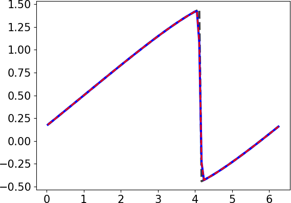
(a) SSP54 and SSP54-GMC

baseline: $\delta=1.64\times 10^{-4}$

GMC: $\delta=1.64\times 10^{-4}$

(b) RK76 and RK76-GMC

Figure 3: Nonlinear Burgers problem (66) with smooth initial data (67). The dashed gray lines depict the exact solution at $t=2$. The WENO-RK solutions calculated on a uniform mesh of $N_{h}=100$ cells without and with GMC limiting are shown as dashed red and solid blue lines, respectively.

5.4 One-dimensional KPP problem

In the last test, we solve the one-dimensional KPP problem [30]. It equips the conservation law

$$\frac{\partial u}{\partial t}+\frac{\partial f(u)}{\partial x}=0\quad\mbox{ in }\quad\Omega=(0,1)$$ (68a)

with the nonlinear and nonconvex flux function

$$f(u)=\begin{cases}\frac{1}{4}u(1-u)&\mbox{ if }u<\frac{1}{2},\\ \frac{1}{2}u(u-1)+\frac{3}{16}&\mbox{ if }\frac{1}{2}\leq u.\end{cases}$$ (68b)

The initial condition is given by [11]

$$u(x,0)=\begin{cases}0&\mbox{ if }x\in[0,0.35],\\ 1&\mbox{ if }x\in(0.35,1].\end{cases}$$ (69)

We define the Lax-Friedrichs fluxes using $\lambda_{i+1/2}=1$ for all $i$. As remarked in [30], many second- and higher-order schemes produce solutions that do not converge to the entropy solution. To show this, we test a fifth-order polynomial reconstruction which yields the interface values

$$\hat{u}_{i}^{+} =\frac{1}{60}(-3u_{i-2}+27u_{i-1}+47u_{i}-13u_{i+1}+2u_{i+2}),$$ (70a)

$$\hat{u}_{i+1}^{-} =\frac{1}{60}(2u_{i-2}-13u_{i-1}+47u_{i}+27u_{i+1}-3u_{i+2}).$$ (70b)

The corresponding non-WENO semi-discretization is combined with the RK76 time integrator. The numerical solutions obtained with the resulting method on different mesh refinement levels are shown in Fig. 4a. Additionally, we perform a grid convergence study and summarize the results in Table 5a. It can be seen that the non-WENO method based on (70) fails to converge to the entropy solution. None of the limiters presented in this work can fix this problem as long as the bounds are global and the baseline scheme is highly oscillatory. However, the combination of the fifth-order WENO space discretization with the RK76 time discretization does converge to the entropy solution even if no limiting is performed; see Fig. 4b and Table 5b. The application of GMC flux limiters removes the small overshoots and undershoots generated by the baseline schemes. The bound-preserving SSP54-GMC and RK76-GMC solutions are shown in Figs 4c and 4d, respectively. Tables 5c and 5d summarize the results of our grid convergence studies for SSP54-GMC and RK76-GMC, respectively.

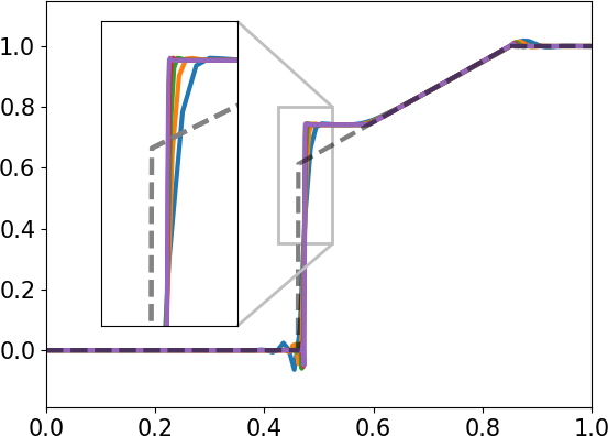
(a) RK76 (non-WENO)

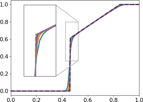
(b) RK76 (WENO)

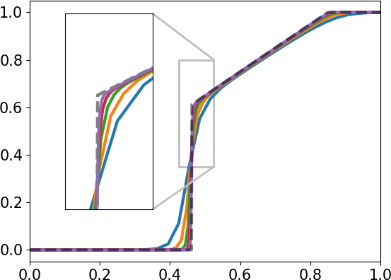
(c) SSP54-GMC

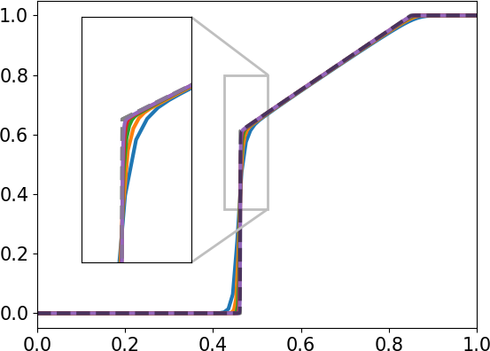
(d) RK76-GMC

Figure 4: Nonlinear problem (68) with non-smooth initial data (69). The exact solution at $t=1$ is shown as a dashed gray line. The remaining curves are numerical solutions obtained on different mesh refinement levels.

$N_{h}$	$E_{1}$	EOC	$\delta$
100	2.22e-02	–	-1.33e-01
200	2.04e-02	0.118	-1.34e-01
400	1.48e-02	0.463	-1.34e-01
800	1.44e-02	0.041	-1.34e-01
1600	1.40e-02	0.040	-1.34e-01

(a) RK76 (non-WENO)

$N_{h}$	$E_{1}$	EOC	$\delta$
100	2.84e-02	–	-3.57e-09
200	1.28e-02	1.15	-4.30e-09
400	7.29e-03	0.81	-3.62e-09
800	3.80e-03	0.93	-4.89e-09
1600	1.98e-03	0.94	-5.34e-09

(b) RK76 (WENO)

$N_{h}$	$E_{1}$	EOC	$\delta$
100	2.84e-02	–	-1.11e-15
200	1.28e-02	1.15	-1.09e-14
400	7.29e-03	0.81	-1.13e-14
800	3.80e-03	0.93	-5.62e-14
1600	1.98e-03	0.94	-5.80e-14

(c) SSP54-GMC

$N_{h}$	$E_{1}$	EOC	$\delta$
100	2.84e-02	–	-1.11e-15
200	1.28e-02	1.15	-1.18e-14
400	7.29e-03	0.81	-1.07e-14
800	3.80e-03	0.93	-5.31e-14
1600	1.98e-03	0.94	-5.31e-14

(d) RK76-GMC

Table 5: Grid convergence study for the nonlinear problem (68) with non-smooth data (69).

6 Conclusions

The convex limiting approaches explored in this work are applicable to a wide range of space discretizations combined with high-order Runge-Kutta time-stepping methods. Although only explicit finite volume schemes were considered in our numerical study, the same flux correction tools can be used to constrain high-order finite element discretizations and implicit RK methods. As shown in [33, 36, 37], convex limiting in space makes it possible to enforce semi-discrete entropy stability conditions in addition to maximum principles. Moreover, the new GMC limiter and its localized prototype proposed in [32] belong to the family of monolithic algebraic flux correction (AFC) schemes which lead to well-posed nonlinear problems and are backed by theoretical analysis [41].

Appendix A High-order baseline RK methods

In this appendix, we provide details of the three high-order explicit baseline RK methods for solving

$$\frac{\mathrm{d}u_{i}}{\mathrm{d}t}=F_{i}(\hat{u}):=-\frac{1}{|K_{i}|}\sum_{j\in\mathcal{N}_{i}}|S_{ij}|H_{ij}(\hat{u}).$$ (71)

A.1 Fourth-order strong stability preserving (SSP54) RK method

The SSP-RK time integrator that we consider in this work is the 4th-order method proposed in [29] and [44]. The Butcher form of its intermediate stages is as follows:

$$y^{(1)} =u^{n}+0.391752226571890\Delta tF(u^{n}),$$

$$y^{(2)} =0.444370493651235u^{n}+0.555629506348765y^{(1)}+0.368410593050371\Delta tF(y^{(1)}),$$

$$y^{(3)} =0.620101851488403u^{n}+0.379898148511597y^{(2)}+0.251891774271694\Delta tF(y^{(2)}),$$

$$y^{(4)} =0.178079954393132u^{n}+0.821920045606868y^{(3)}+0.544974750228521\Delta tF(y^{(3)}),$$

$$y^{(5)} =0.517231671970585y^{(2)}+0.096059710526147y^{(3)}+0.063692468666290\Delta tF(y^{(3)})$$

$$+0.386708617503269y^{(4)}+0.226007483236906\Delta tF(y^{(4)}).$$

Note that each stage is a convex combination of Euler steps. Therefore, if $F(\cdot)$ is a BP spatial discretization and $u^{n}$ is BP, then each stage is BP under appropriate time step restrictions. The RK update is given by $u^{n+1}=y^{(5)}$. Hence, if the stages are BP, $u^{n+1}$ is BP and no extra limiting is needed.

A.2 Fifth-order extrapolated Euler (ExE-RK5) RK method

The Butcher tableau of the 5th-order extrapolated Euler RK method is given by

(84)

The intermediate stages (written in Shu-Osher and Butcher form) are as follows:

$$y^{(1)} =u^{n} \approx u(t^{n}),$$

$$y^{(2)} =y^{(1)}+\frac{1}{2}\Delta tF(y^{(1)}) \approx u(t^{n}+\Delta t/2),$$

$$y^{(3)} =y^{(1)}+\frac{1}{3}\Delta tF(y^{(1)}) \approx u(t^{n}+\Delta t/3),$$

$$y^{(4)} =y^{(3)}+\frac{1}{3}\Delta tF(y^{(3)})=y^{(1)}+\frac{\Delta t}{3}[F(y^{(1)})+F(y^{(3)})] \approx u(t^{n}+2\Delta t/3),$$

$$y^{(5)} =y^{(1)}+\frac{1}{4}\Delta tF(y^{(1)}) \approx u(t^{n}+\Delta t/4),$$

$$y^{(6)} =y^{(5)}+\frac{1}{4}\Delta tF(y^{(5)})=y^{(1)}+\frac{\Delta t}{4}[F(y^{(1)})+F(y^{(5)})] \approx u(t^{n}+\Delta t/2),$$

$$y^{(7)} =y^{(6)}+\frac{1}{4}\Delta tF(y^{(6)})=y^{(1)}+\frac{\Delta t}{4}[F(y^{(1)})+F(y^{(5)})+F(y^{(6)})] \approx u(t^{n}+3\Delta t/4),$$

$$y^{(8)} =y^{(1)}+\frac{1}{5}\Delta tF(y^{(1)}) \approx u(t^{n}+\Delta t/5),$$

$$y^{(9)} =y^{(8)}+\frac{1}{5}\Delta tF(y^{(8)})=y^{(1)}+\frac{\Delta t}{5}[F(y^{(1)})+F(y^{(8)})] \approx u(t^{n}+2\Delta t/5),$$

$$y^{(10)} =y^{(9)}+\frac{1}{5}\Delta tF(y^{(9)})=y^{(1)}+\frac{\Delta t}{5}[F(y^{(1)})+F(y^{(8)})+F(y^{(9)})] \approx u(t^{n}+3\Delta t/5),$$

$$y^{(11)} =y^{(10)}+\frac{1}{5}\Delta tF(y^{(10)})=y^{(1)}+\frac{\Delta t}{5}[F(y^{(1)})+F(y^{(8)})+F(y^{(9)})+F(y^{(10)})] \approx u(t^{n}+4\Delta t/5).$$

Note that if $F(\cdot)$ is a BP spatial discretization and $u^{n}$ is BP, then each stage of this ExE-RK method is BP under appropriate time step restrictions. The approximations $y^{(1)}$, $y^{(2)}$, $y^{(3)}$, $y^{(5)}$, and $y^{(8)}$ are BP because they correspond to forward Euler updates of $u^{n}$. The remaining stages are BP since $y^{(m)}$ is a forward Euler update of a BP approximation $y^{(r)}$ for some $r\in\{1,\ldots,m-1\}$.

The Aitken-Neville interpolation yields the temporally 5th-order approximation

$$u^{\rm RK}= \frac{1}{24}\left[y^{(1)}+\Delta tF(y^{(1)})\right]-\frac{8}{3}\left[y^{(2)}+\frac{1}{2}\Delta tF(y^{(2)})\right]+\frac{81}{4}\left[y^{(4)}+\frac{1}{3}\Delta tF(y^{(4)})\right]$$

$$-\frac{128}{3}\left[y^{(7)}+\frac{1}{4}\Delta tF(y^{(7)})\right]+\frac{625}{24}\left[y^{(11)}+\frac{1}{5}\Delta tF(y^{(11)})\right].$$

Note that this Euler extrapolation method combines $S=5$ first-order approximations of $u^{n+1}$. Since this combination is not convex, $u^{\rm RK}$ is not necessarily BP even if $y^{(1)},\ldots,y^{(11)}$ are BP. To enforce the BP property of the final solution, we perform flux limiting using the Butcher form representation

$$u^{\rm RK}=u^{n}+\Delta t\Big{[} -\frac{4}{3}F(y^{(2)})+\frac{27}{4}F(y^{(3)})+\frac{27}{4}F(y^{(4)})-\frac{32}{3}F(y^{(5)})-\frac{32}{3}F(y^{(6)})-\frac{32}{3}F(y^{(7)})$$

$$+\frac{125}{24}F(y^{(8)})+\frac{125}{24}F(y^{(9)})+\frac{125}{24}F(y^{(10)}+\frac{125}{24}F(y^{(11)})\Big{]}.$$ (85)

A.3 Sixth-order (RK76) RK method

This 6th-order RK method, proposed in [8], consists of seven stages and has the Butcher tableau

(94)

The intermediate stages of this method are not Euler steps. If we require them to be BP, the numerical fluxes $H_{ij}$ should be constrained using the limiters from Section 3.3 in each stage. The BP property of the final solution $u^{\rm RK}$ can be enforced similarly using the limiter from Section 3.2.

Appendix B Flux-limited WENO discretization in 1D

In this appendix, we provide details of flux-corrected RK methods for one-dimensional hyperbolic conservation laws of the form $\frac{\partial u}{\partial t}+\frac{\partial f(u)}{\partial x}=0$. Although the underlying low-order and high-order approximations are of little interest per se, we present their one-dimensional formulations as well. We assume the mesh is uniform and, therefore, the mesh size $|K_{i}|=\Delta x$ is constant.

B.1 The low-order method

In one space dimension, the common interface $S_{ij}$ of control volumes with indices $i$ and $j=i+1$ is the point $x_{i+1/2}=\frac{1}{2}(x_{i}+x_{i+1})$. The 1D version of the FE-LLF approximation (38) is given by

$$u_{i}^{\rm FE}=u_{i}^{n}-\frac{\Delta t}{\Delta x}[H^{\rm FE}_{i+1/2}-H^{\rm FE}_{i-1/2}],$$ (95)

where

$$H^{\rm FE}_{i+1/2}=\frac{f(u_{i}^{n})+f(u_{i+1}^{n})}{2}-\lambda_{i+1/2}\frac{u_{i+1}^{n}-u_{i}^{n}}{2}$$

is the first-order numerical flux and $\lambda_{i+1/2}$ is an upper bound for the wave speed of the Riemann problem associated with the states $u_{i}^{n}$ and $u_{i+1}^{n}$. The bar state form of (95) is given by

$$u_{i}^{\rm FE}=u_{i}^{n}+\frac{\Delta t}{\Delta x}[\lambda_{i+1/2}(\bar{u}^{L}_{i+1/2}-u_{i}^{n})+\lambda_{i-1/2}(\bar{u}^{L}_{i-1/2}-u_{i}^{n})]=u_{i}^{n}+\frac{\Delta t}{\Delta x}d_{i}(\bar{u}_{i}^{L}-u_{i}^{n}),$$

where

$$\bar{u}_{i+1/2}^{L}=\frac{u_{i+1}^{n}+u_{i}^{n}}{2}-\frac{f(u_{i+1}^{n})-f(u_{i}^{n})}{2\lambda_{i+1/2}},\qquad\bar{u}_{i-1/2}^{L}=\frac{u_{i}^{n}+u_{i-1}^{n}}{2}+\frac{f(u_{i-1}^{n})-f(u_{i}^{n})}{2\lambda_{i-1/2}},$$

$$\bar{u}_{i}^{L}=\frac{1}{d_{i}}[\lambda_{i+1/2}\bar{u}_{i+1/2}^{L}+\lambda_{i-1/2}\bar{u}_{i-1/2}^{L}],\qquad d_{i}=\lambda_{i+1/2}+\lambda_{i-1/2}.$$

This representation proves that the method is bound-preserving (BP) with respect to the local bounds $u_{i}^{\max}=\max\{u_{i-1}^{n},u_{i}^{n},u_{i+1}^{n}\}$ and $u_{i}^{\min}=\min\{u_{i-1}^{n},u_{i}^{n},u_{i+1}^{n}\}$, provided

$$\Delta t\leq\frac{\Delta x}{\lambda_{i+1/2}+\lambda_{i-1/2}}.$$ (96)

However, the method is only first-order accurate in space and time.

B.2 The baseline high-order method

The unlimited form of an explicit Runge-Kutta method (with a WENO discretization) is given by

$$u_{i}^{\rm RK}=u_{i}^{n}-\frac{\Delta t}{\Delta x}[H_{i+1/2}^{\text{RK}}-H_{i-1/2}^{\text{RK}}],\qquad H_{i+1/2}^{\text{RK}}=\sum_{m=1}^{M}b_{m}H_{i+1/2}^{(m)},$$ (97)

where $M$ is the number of stages of the RK method and $b_{m}$ are the Butcher weights of the final RK update. The Lax-Friedrichs flux $H_{i+1/2}^{(m)}=H\big{(}\hat{y}_{i}^{(m)}(x_{i+1/2}),\hat{y}_{i+1}^{(m)}(x_{i+1/2}),1\big{)}$ is calculated using the interface values of the high-order WENO reconstructions $\hat{y}^{(m)}_{i}(x)$ and $\hat{y}^{(m)}_{i+1}(x)$ in cells $K_{i}$ and $K_{i+1}$, respectively. These WENO reconstructions are obtained from the $m$-th stage cell averages

$$y_{i}^{(m)}=u_{i}^{n}-\frac{\Delta t}{\Delta x}\sum_{s=1}^{m-1}a_{ms}\big{[}H_{i+1/2}^{(s)}-H_{i-1/2}^{(s)}\big{]},$$ (98)

where $a_{ms},\ s=1,\ldots,m-1$ are the coefficients of the $m$-th row in the Butcher tableau (56). Method (97) is high-order in space and time. In particular, we combine a fifth-order WENO spatial discretization with the three explicit RK methods in A. The use of WENO numerical fluxes produces a solution which is typically (almost) non-oscillatory. However, this solution is not BP in general.

B.3 Spatial GMC limiting in 1D

Let us now apply the GMC space limiters from Section 2 to the high-order semi-discretization

$$\Delta x\frac{\mathrm{d}u_{i}}{\mathrm{d}t}=-[H_{i+1/2}^{\rm WENO}-H_{i-1/2}^{\rm WENO}],$$ (99)

where $H_{i+1/2}^{\rm WENO}=H(\hat{u}_{i}(x_{i+1/2}),\hat{u}_{i+1}(x_{i+1/2}),1)$ is the high-order WENO flux. Using the corresponding low-order flux $H_{i+1/2}^{\rm LLF}=H(u_{i},u_{i+1},1)$, the baseline scheme (99) can be written as

$$\Delta x\frac{\mathrm{d}u_{i}}{\mathrm{d}t}=-\big{[}\big{(}H_{i+1/2}^{\rm LLF}-F_{i+1/2}\big{)}-\big{(}H_{i-1/2}^{\rm LLF}-F_{i-1/2}\big{)}\big{]}.$$ (100)

The one-dimensional GMC limiter replaces the antidiffusive flux $F_{i+1/2}=H_{i+1/2}^{\rm LLF}-H_{i+1/2}^{\rm WENO}$ by its limited counterpart $F_{i+1/2}^{*}=\alpha_{i+1/2}F_{i+1/2}$. The correction factor $\alpha_{i+1/2}$ is calculated as follows:

$$P^{+}_{i} =\max\{0,F_{i+1/2}\}+\max\{0,-F_{i-1/2}\}, P^{-}_{i} =\min\{0,F_{i+1/2}\}+\min\{0,-F_{i-1/2}\},$$ (101a)

$$Q_{i}^{+} =d_{i}(u^{\max}_{i}-\bar{u}_{i}^{L})+\gamma(u^{\max}_{i}-u_{i}^{n}), Q_{i}^{-} =d_{i}(u^{\min}_{i}-\bar{u}_{i}^{L})+\gamma d_{i}(u^{\min}_{i}-u_{i}^{n}),$$ (101b)

$$R^{\pm}_{i} =\begin{cases}1&\mbox{if }\phantom{|}P^{\pm}_{i}\phantom{|}=0,\\ \min\left\{1,\frac{Q_{i}^{\pm}}{P_{i}^{\pm}}\right\}&\mbox{if }|P^{\pm}_{i}|>0,\end{cases} \alpha_{i+1/2} =\begin{cases}\min\{R^{+}_{i},R^{-}_{i+1}\}&\mbox{ if }\ F_{i+1/2}>0,\\ \min\{R^{-}_{i},R^{+}_{i+1}\}&\mbox{ if }\ F_{i+1/2}\leq 0.\end{cases}$$ (101c)

An SSP-RK time discretization of the flux-corrected WENO scheme

$$\Delta x\frac{\mathrm{d}u_{i}}{\mathrm{d}t}=-\big{[}\big{(}H_{i+1/2}^{\rm LLF}-F_{i+1/2}^{*}\big{)}-\big{(}H_{i-1/2}^{\rm LLF}-F_{i-1/2}^{*}\big{)}\big{]}$$ (102)

is BP under the time step restriction

$$\Delta t\leq\frac{\mu(1+\gamma)\Delta x}{\lambda_{i+1/2}+\lambda_{i-1/2}},$$ (103)

where $\mu\in(0,1]$ is the SSP coefficient of the RK method and $\gamma\geq 0$ is the GMC relaxation parameter.

B.4 Space-time GMC limiting in 1D

The final stage (97) of a baseline high-order WENO-RK scheme can be written as

$$u_{i}^{\rm RK}=u_{i}^{n}-\frac{\Delta t}{\Delta x}\big{[}H_{i+1/2}^{\text{RK}}-H_{i-1/2}^{\text{RK}}\big{]}=u_{i}^{n}-\frac{\Delta t}{\Delta x}\big{[}(H^{\rm FE}_{i+1/2}-F^{\rm RK}_{i+1/2})-(H^{\rm FE}_{i-1/2}-F^{\rm RK}_{i-1/2}\big{)}\big{]},$$

where $F^{\rm RK}_{i+1/2}=H_{i+1/2}^{{\rm FE}}-H_{i+1/2}^{{\rm RK}}$ is the raw antidiffusive flux. Using this representation, space-time GMC limiting can be performed as in B.3 using $H^{\rm FE}_{i+1/2}$ in place of $H^{\rm LLF}_{i+1/2}$ and $F^{\rm RK}_{i+1/2}$ in place of $F_{i+1/2}$. The implementation of GMC for intermediate RK stages is similar.

Remark 7.

The FCT version of the space-time limiter uses $u_{i}^{\rm FE}$ defined by (95) to construct

$$Q_{i}^{+}=\frac{\Delta x}{\Delta t}(u^{\max}_{i}-u_{i}^{\rm FE}),\qquad Q_{i}^{-}=\frac{\Delta x}{\Delta t}(u^{\min}_{i}-u_{i}^{\rm FE})$$

for calculation of the correction factors $R_{i}^{\pm}$ and $\alpha_{ij}$ in (101c).

References

- [1] T. Arbogast, C.-S. Huang, X. Zhao, and D. N. King, A third order, implicit, finite volume, adaptive Runge–Kutta WENO scheme for advection-diffusion equations. Computer Methods Appl. Mech. Engrg. 368 (2020) 113155.
- [2] T. Barth and D.C. Jespersen, The design and application of upwind schemes on unstructured meshes. AIAA Paper, 89-0366, 1989.
- [3] F. Blanchini, Set invariance in control. Automatica 35(11) (1999) 1747–1767.
- [4] K. Deimling, Ordinary differential equations in Banach spaces (Vol. 596). (2006) Springer.
- [5] J.P. Boris and D.L. Book, Flux-Corrected Transport: I. SHASTA, a fluid transport algorithm that works. J. Comput. Phys. 11 (1973) 38–69.
- [6] Z. Horváth, Invariant cones and polyhedra for dynamical systems. In Proceeding of the International Conference in Memoriam Gyula Farkas (2005) 65–74.
- [7] T. A. Burton, A fixed-point theorem of Krasnoselskii. Appl. Math. Lett. 11 (1998) 85–88.
- [8] J. C. Butcher, On Runge-Kutta processes of high order. J. of the Australian Mathematical Society 4-2, (1964) 179–194.
- [9] C.J. Cotter and D. Kuzmin, Embedded discontinuous Galerkin transport schemes with localised limiters. J. Comput. Phys. 311 (2016) 363–373.
- [10] K. Duraisamy, K. Baeder, and J.-G. Liu, Concepts and application of time-limiters to high resolution schemes. J. of Sci. Comput. 19 (2003) 139–162.
- [11] A. Ern and J.-L. Guermond, Weighting the edge stabilization. SIAM J. Numer. Anal. 51 (2013) 1655–1677.
- [12] D. Feng, I. Neuweiler, U. Nackenhorst, and T. Wick, A time-space flux-corrected transport finite element formulation for solving multi-dimensional advection-diffusion-reaction equations. J. Comput. Phys. 396 (2019) 31-53.
- [13] S. Gottlieb, D. Ketcheson, and C.-W. Shu, Strong Stability Preserving Runge-Kutta and Multistep Time Discretizations. World Scientific, 2011.
- [14] S. Gottlieb, C.-W. Shu, and E. Tadmor, Strong stability-preserving high-order time discretization methods. SIAM Review 43 (2001) 89–112.
- [15] J.-L. Guermond, M. Nazarov, B. Popov, and I. Tomas, Second-order invariant domain preserving approximation of the Euler equations using convex limiting. SIAM J. Sci. Computing 40 (2018) A3211-A3239.
- [16] J.-L. Guermond, R. Pasquetti, and B. Popov, Entropy viscosity method for nonlinear conservation laws. J. Comput. Phys. 230 (2011) 4248–4267.
- [17] J.-L. Guermond and B. Popov, Invariant domains and first-order continuous finite element approximation for hyperbolic systems. SIAM J. Numer. Anal. 54 (2016) 2466–2489.
- [18] E. Hairer, S. P. Norsett, and G. Wanner, Solving Ordinary Differential Equations I: Nonstiff Problems. Second edition, Springer, 1993.
- [19] R. Anderson, V. Dobrev, Tz. Kolev, D. Kuzmin, M. Quezada de Luna, R. Rieben, and V. Tomov, High-order local maximum principle preserving (MPP) discontinuous Galerkin finite element method for the transport equation. J. Comput. Phys. 334 (2017) 102–124.
- [20] H. Hajduk, Monolithic convex limiting in discontinuous Galerkin discretizations of hyperbolic conservation laws. Preprint arXiv:2007.01212 [math.NA], 2020.
- [21] A. Harten, High resolution schemes for hyperbolic conservation laws. J. Comput. Phys. 49 (1983) 357–393.
- [22] A. Harten, On a class of high resolution total-variation-stable finite-difference-schemes. SIAM J. Numer. Anal. 21 (1984) 1-23.
- [23] X.Y. Hu, N. A. Adams, and C.-W. Shu, Positivity-preserving method for high-order conservative schemes solving compressible Euler equations. J. Comput. Phys. 242 (2013) 169–180.
- [24] W. Hundsdorfer, D. I. Ketcheson, and I. Savostianov, Error analysis of explicit partitioned Runge-Kutta schemes for conservation laws. J. Sci. Comput. 63 (2015) 633–653.
- [25] A. Jameson, Computational algorithms for aerodynamic analysis and design. Appl. Numer. Math. 13 (1993) 383–422.
- [26] A. Jameson, Positive schemes and shock modelling for compressible flows. Int. J. Numer. Methods Fluids 20 (1995) 743-776.
- [27] D. I. Ketcheson, C. B. MacDonald, and S. J. Ruuth, Spatially partitioned embedded Runge-Kutta methods. SIAM J. Numer. Anal. 51 (2013) 2887–2910.
- [28] D. I. Ketcheson and U. bin Waheed, A comparison of high-order explicit Runge-Kutta, extrapolation, and deferred correction methods in serial and parallel. Comm. App. Math. and Comp. Sci. 9 (2014) 175–200.
- [29] J. F. B. M. Kraaijevanger, Contractivity of Runge-Kutta methods. BIT, 31 (1991) 482–528.
- [30] A. Kurganov, G. Petrova, and B. Popov, Adaptive semidiscrete central-upwind schemes for nonconvex hyperbolic conservation laws. SIAM J. Sci. Comput. 29 (2007) 2381–2401.
- [31] A. Kurganov and E. Tadmor, New high-resolution central schemes for nonlinear conservation laws and convection-diffusion equations. J. Comput. Phys. 160 (2000) 241–282.
- [32] D. Kuzmin, Monolithic convex limiting for continuous finite element discretizations of hyperbolic conservation laws. Comput. Methods Appl. Mech. Engrg. 361 (2020) 112804.
- [33] D. Kuzmin, Entropy stabilization and property-preserving limiters for discontinuous Galerkin discretizations of scalar hyperbolic problems. J. Numer. Math. (2020), https://doi.org/10.1515/jnma-2020-0056.
- [34] D. Kuzmin, A new perspective on flux and slope limiting in discontinuous Galerkin methods for hyperbolic conservation laws. Comput. Methods Appl. Mech. Engrg. 373 (2021) 113569.
- [35] D. Kuzmin, H. Hajduk, and A. Rupp, Locally bound-preserving enriched Galerkin methods for the linear advection equation. Computers & Fluids 205 (2020) 104525.
- [36] D. Kuzmin and M. Quezada de Luna, Algebraic entropy fixes and convex limiting for continuous finite element discretizations of scalar hyperbolic conservation laws. Comput. Methods Appl. Mech. Engrg. 372 (2020) 113370.
- [37] D. Kuzmin and M. Quezada de Luna, Entropy conservation property and entropy stabilization of high-order continuous Galerkin approximations to scalar conservation laws. Computers & Fluids 213 (2020) 104742.
- [38] D. Kuzmin, M. Quezada de Luna, and C. Kees, A partition of unity approach to adaptivity and limiting in continuous finite element methods. Computers & Math. with Applications 78 (2019) 944–957.
- [39] J.-L. Lee, R. Bleck, and A. E. MacDonald, A multistep flux-corrected transport scheme. J. Comput. Phys. 229 (2010) 9284–9298.
- [40] R.J. LeVeque, Finite Volume Methods for Hyperbolic Problems. Cambridge University Press, 2002.
- [41] C. Lohmann, Physics-Compatible Finite Element Methods for Scalar and Tensorial Advection Problems. Springer Spektrum, 2019.
- [42] C. Lohmann, D. Kuzmin, J.N. Shadid, and S. Mabuza, Flux-corrected transport algorithms for continuous Galerkin methods based on high order Bernstein finite elements. J. Comput. Phys. 344 (2017) 151-186.
- [43] C.-W. Shu, High order weighted essentially nonoscillatory schemes for convection dominated problems. SIAM Review 51 (2009) 82–126.
- [44] R. J. Spiteri and S. J. Ruuth, A new class of optimal high-order strong stability-preserving time discretization methods. SIAM J. Numer. Anal. 40 (2002) 469–491.
- [45] S.T. Zalesak, Fully multidimensional flux-corrected transport algorithms for fluids. J. Comput. Phys. 31 (1979) 335–362.
- [46] X. Zhang and C.-W. Shu, On positivity-preserving high order discontinuous Galerkin schemes for compressible Euler equations on rectangular meshes. J. Comput. Phys. 229 (2010) 8918–8934.
- [47] X. Zhang and C.-W. Shu, Maximum-principle-satisfying and positivity-preserving high-order schemes for conservation laws: survey and new developments. Proceedings of the Royal Society A: Mathematical, Physical and Engineering Sciences 467 (2011) 2752–2776.