From Two-Class Linear Discriminant Analysis to
Interpretable Multilayer Perceptron Design

Abstract

A closed-form solution exists in two-class linear discriminant analysis (LDA), which discriminates two Gaussian-distributed classes in a multi-dimensional feature space. In this work, we interpret the multilayer perceptron (MLP) as a generalization of a two-class LDA system so that it can handle an input composed by multiple Gaussian modalities belonging to multiple classes. Besides input layer $l_{in}$ and output layer $l_{out}$, the MLP of interest consists of two intermediate layers, $l_{1}$ and $l_{2}$. We propose a feedforward design that has three stages: 1) from $l_{in}$ to $l_{1}$: half-space partitionings accomplished by multiple parallel LDAs, 2) from $l_{1}$ to $l_{2}$: subspace isolation where one Gaussian modality is represented by one neuron, 3) from $l_{2}$ to $l_{out}$: class-wise subspace mergence, where each Gaussian modality is connected to its target class. Through this process, we present an automatic MLP design that can specify the network architecture (i.e., the layer number and the neuron number at a layer) and all filter weights in a feedforward one-pass fashion. This design can be generalized to an arbitrary distribution by leveraging the Gaussian mixture model (GMM). Experiments are conducted to compare the performance of the traditional backpropagation-based MLP (BP-MLP) and the new feedforward MLP (FF-MLP).

I Introduction

The multilayer perceptron (MLP), proposed by Rosenblatt in 1958 [1], has a history of more than 60 years. However, while there are instances of theoretical investigations into why the MLP works (e.g., the classic articles of Cybenko [2], and Hornik, Stinchcombe and White [3]), the majority of the efforts have focused on applications such as speech recognition [4], economic time series [5], image processing [6], and many others.

One-hidden-layer MLPs with suitable activation functions are shown to be universal approximators [2, 3, 7]. Yet, this only shows the existence but does not provide guideline in network design [8]. Sometimes, deeper networks could be more efficient than shallow wider networks. The MLP design remains to be an open problem. In practice, trials and errors are made in determining the layer number and the neuron number of each layer. The process of hyper parameter finetuning is time consuming. We attempt to address these two problems simultaneously in this work: MLP theory and automatic MLP network design.

For MLP theory, we will examine the MLP from a brand new angle. That is, we view an MLP as a generalization form of the classical two-class linear discriminant analysis (LDA). The input to a two-class LDA system is two Gaussian distributed sources, and the output is the predicted class. The two-class LDA is valuable since it has a closed-form solution. Yet, its applicability is limited due to the severe constraint in the problem set-up. It is desired to generalize the LDA so that an arbitrary combination of multimodal Gaussian sources represented by multiple object classes can be handled. If there exists such a link between MLP and two-class LDA, analytical results of the two-class LDA can be leveraged for the understanding and design of the MLP. The generalization is possible due to the following observations.

• The first MLP layer splits the input space with multiple partitioning hyperplanes. We can also generate multiple partitioning hyperplanes with multiple two-class LDA systems running in parallel.

• With specially designed weights, each neuron in the second MLP layer can activate one of the regions formed by the first layer hyperplanes.

• A sign confusion problem arises when two MLP layers are in cascade. This problem is solved by applying the rectified linear unit (ReLU) operation to the output of each layer.

In this paper, we first make an explicit connection between the two-class LDA and the MLP design. Then, we propose a general MLP architecture that contains input layer $l_{in}$, output layer $l_{out}$, two intermediate layers, $l_{1}$ and $l_{2}$. Our MLP design consists of three stages:

• Stage 1 (from input layer $l_{in}$ to $l_{1}$): Partition the whole input space flexibly into a few half-subspace pairs, where the intersection of half-subspaces yields many regions of interest.

• Stage 2 (from intermediate layer $l_{1}$ to $l_{2}$): Isolate each region of interest from others in the input space.

• Stage 3 (from intermediate layer $l_{2}$ to output layer $l_{out}$): Connect each region of interest to its associated class.

The proposed design can determine the MLP architecture and weights of all links in a feedforward one-pass manner without trial and error. No backpropagation is needed in network training.

In contrast with traditional MLPs that are trained based on end-to-end optimization through backpropagation (BP), it is proper to call our new design the feedforward MLP (FF-MLP) and traditional ones the backpropagation MLP (BP-MLP). Intermediate layers are not hidden but explicit in FF-MLP. Experiments are conducted to compare the performance of FF-MLPs and BP-MLPs. The advantages of FF-MLPs over BP-MLPs are obvious in many areas, including faster design time and training time.

The rest of the paper is organized as follows. The relationship between the two-class LDA and the MLP is described in Sec. II. A systematic design of an interpretable MLP in a one-pass feedforward manner is presented in Sec. III. Several MLP design examples are given in Sec. IV. Observations on the BP-MLP behavior are stated in Sec. V. We compare the performance of BP-MLP and FF-MLP by experiments in Sec. VI. Comments on related previous work are made in Sec. VII. Finally, concluding remarks and future research directions are given in Sec. VIII.

II From Two-Class LDA to MLP

II-A Two-Class LDA

Without loss of generality, we consider two-dimensional (2D) random vectors, denoted by ${\bf x}\in R^{2}$, as the input for ease of visualization. They are samples from two classes, denoted by $C_{1}$ and $C_{2}$, each of which is a Gaussian-distributed function. The two distributions can be expressed as $\mathcal{N}(\mu_{1},\Sigma_{1})$ and $\mathcal{N}(\mu_{2},\Sigma_{2})$, where $\bm{\mu_{1}}$ and $\bm{\mu_{2}}$ are their mean vectors and $\bm{\Sigma_{1}}$ and $\bm{\Sigma_{2}}$ their covariance matrices, respectively. Fig. 1(a) shows an example of two Gaussian distributions, where the blue and orange dots are samples from classes $C_{1}$ and $C_{2}$, respectively. Each Gaussian-distributed modality is called a Gaussian blob.

(a)

(b)

Figure 1: Illustration of (a) two Gaussian blobs separated by a line in a 2D plane, and (b) a one-layer two-neuron perceptron system.

A linear classifier can be used to separate the two blobs, known as the two-class linear discriminant analysis (LDA), in closed form. LDA assumes homoscedasticity, that is, the covariances of different classes are identical: $\bm{\Sigma_{1}}=\bm{\Sigma_{2}}=\bm{\Sigma}$. In this case, the decision boundary can be formulated into the form of [9][10]

$$\bm{w}^{T}\bm{x}+b=0,$$ (1)

where

$${\bf w}=(w_{1},w_{2})^{T}=\bm{\Sigma}^{-1}(\bm{\mu_{1}}-\bm{\mu_{2}}).$$ (2)

$$b=\frac{1}{2}\bm{\mu_{2}}^{T}\bm{\Sigma}^{-1}\bm{\mu_{2}}-\frac{1}{2}\bm{\mu_{1}}^{T}\bm{\Sigma}^{-1}\bm{\mu_{1}}+\log{\frac{p}{1-p}},$$ (3)

where $p=P(y=1)$. Then, sample ${\bf x}$ is classified to class $C_{1}$ if $\bm{w}^{T}\bm{x}+b$ evaluates positive. Otherwise, sample ${\bf x}$ is classified to class $C_{2}$.

II-B One-Layer Two-Neuron Perceptron

We can convert the LDA in Sec. II-A to a one-layer two-neuron perceptron system as shown in Fig. 1(b). The input consists of two nodes, denoting the first and the second dimensions of random vector ${\bf x}$. The output consists of two neurons in orange and green, respectively. The two orange links have weight $w_{1}$ and $w_{2}$ that can be determined based on Eq. (2). The bias $b$ for the orange node can be obtained based on Eq. (3). Similarly, the two green links have weight $-w_{1}$ and $-w_{2}$ and the green node has bias $-b$. The rectified linear unit (ReLU), defined as

$$\mbox{ReLU}(y)=\max(0,y),$$ (4)

is chosen to be the activation function in the neuron. The activated responses of the two neurons are shown in the right part of Fig. 1(b). The left (or right) dark purple region in the top (or bottom) subfigure means zero responses. Responses are non-zero in the other half. We see more positive values as moving further to the right (or left).

One may argue that there is no need to have two neurons in Fig. 1(b). One neuron is sufficient in making correct decision. Although this could be true, some information of the two-class LDA system is lost in a one-neuron system. The magnitude of the response value for samples in the left region is all equal to zero if only the orange output node exists. This degrades the classification performance. In contrast, by keeping both orange and green nodes, we can preserve the same amount of information as that in the two-class LDA.

One may also argue that there is no need to use the ReLU activation function in this example. Yet, ReLU activation is essential when the one-layer perceptron is generalized to a multi-layer perceptron as explained below. We use $\tilde{{\bf x}}$ to denote the mirror (or the reflection) of ${\bf x}$ against the decision line in Fig. 1(a) as illustrated by the pair of green dots. Clearly, their responses are of the opposite sign. The neuron response in the next stage is the sum of multiple response-weight products. Then, one cannot distinguish the following two cases:

• a positive response multiplied by a positive weight,

• a negative response multiplied by a negative weight;

since both contribute to the output positively. Similarly, one cannot distinguish the following two cases, either:

• a positive response multiplied by a negative weight,

• a negative response multiplied by a positive weight;

since both contribute to the output negatively. As a result, the roles of ${\bf x}$ and its mirror $\tilde{{\bf x}}$ are mixed together. The sign confusion problem was first pointed out in [11]. This problem can be resolved by the ReLU nonlinear activation.

II-C Need of Multilayer Perceptron

(a)

(b)

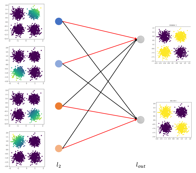
(c)

Figure 2: MLP design for Example 1 (XOR): (a) weights between input layer $l_{in}$ and layer $l_{1}$, (b) weights between layer $l_{1}$ and layer $l_{2}$, where red links represent weight of 1 and black links represent weights $-P$, where $P$ is assumed to be a sufficiently large positive number, (c) weights between $l_{2}$ and $l_{out}$, where red links represent weight of 1 and black links represent weight of 0.

Samples from multiple classes cannot be separated by one linear decision boundary in general. One simple example is given below.

Example 1 (XOR). The sample distribution of the XOR pattern is given in Fig. 2(a). It has four Gaussian blobs belonging to two classes. Each class corresponds to the “exclusive-OR” output of coordinates’ signs of inputs of a blob. That is, Gaussian blobs located in the quadrant where x-axis and y-axis have the same sign belong to class 0. Otherwise, they belong to class 1. The MLP has $l_{in}$, $l_{1}$, $l_{2}$ and $l_{out}$ four layers and three stages of links. We will examine the design stage by stage in a feedforward manner.

II-C1 Stage 1 (from $l_{in}$ to $l_{1}$)

Two partitioning lines are needed to separate four Gaussian blobs – one vertical and one horizontal ones as shown in the figure. Based on the discussion in Sec. II-A, we can determine two weight vectors, ${\bf w^{\prime}}$ and ${\bf w^{\prime\prime}}$, which are vectors orthogonal to the vertical and horizontal lines, respectively. In other words, we have two LDA systems that run in parallel between the input layer and the first intermediate layer of the MLP as shown in Fig. 2(a). Layer $l_{1}$ has four neurons. They are partitioned into two pairs of similar color: blue and light blue as one pair and orange and light orange as another pair. The responses of these four neurons are shown in the figure. By appearance, the dimension goes from two to four from $l_{in}$ to $l_{1}$. Actually, each pair of nodes offers a complementary representation in one dimension. For example, the blue and light blue nodes cover the negative and the positive regions of the horizontal axis, respectively.

II-C2 Stage 2 (from $l_{1}$ to $l_{2}$)

To separate four Gaussian blobs in Example 1 completely, we need layer $l_{2}$ as shown in Fig. 2(b). The objective is to have one single Gaussian blob represented by one neuron in layer $l_{2}$. We use the blob in the first quadrant as an example. It is the top node in layer $l_{2}$. The light blue and the orange nodes have nonzero responses in this region, and we can set their weights to 1 (in red). There is however a side effect - undesired responses in the second and the fourth quadrants are brought in as well. The side effect can be removed by subtracting responses from the blue and the light orange nodes. In Fig. 2(b), we use red and black links to represent weight of $1$ and $-P$, where $P$ is assumed to be a sufficiently large positive number, respectively. With this assignment, we can preserve responses in the first quadrant and make responses in the other three quadrants negative. Since negative responses are clipped to zero by ReLU, we obtain the desired response.

II-C3 Stage 3 (from $l_{2}$ to $l_{out}$)

The top two nodes belong to one class and the bottom two nodes belong to another class in this example. The weight of a link is set to one if it connects a Gaussian blob to its class. Otherwise, it is set to zero. All bias terms are zero.

III Design of Feedforward MLP (FF-MLP)

In this section, we generalize the MLP design for Example 1 so that it can handle an input composed by multiple Gaussian modalities belonging to multiple classes. The feedforward design procedure is stated in Sec. III-A. Pruning of partitioning hyperplanes is discussed in Sec. III-B. Finally, the designed FF-MLP architecture is summarized in Sec. III-C.

III-A Feedfoward Design Procedure

We examine an $N$-dimensional sample space formed by $G$ Gaussian blobs belonging to $C$ classes, where $G\geq C$. The MLP architecture is shown in Fig. 3. Again, it has layers $l_{in}$, $l_{1}$, $l_{2}$ and $l_{out}$. Their neuron numbers are denoted by $D_{in}$, $D_{1}$, $D_{2}$ and $D_{out}$, respectively. Clearly, we have

$$D_{in}=N,\quad D_{out}=C.$$ (5)

We will show that

$$D_{1}\leq 2\left(\begin{array}[]{c}G\\ 2\end{array}\right),\quad G\leq D_{2}\leq 2^{G(G-1)/2}.$$ (6)

We examine the following three stages one more time but in a more general setting.

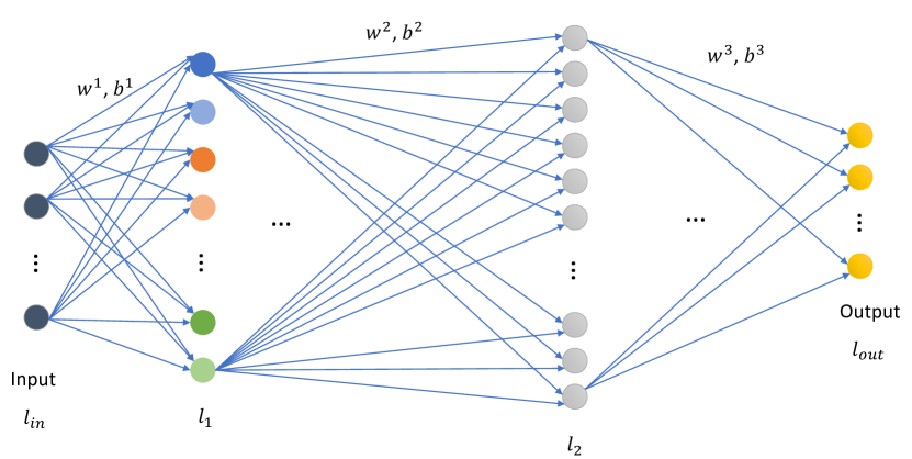
Figure 3: Proposed MLP design: the MLP network with $l_{1}$ and $l_{2}$ two intermediate layers, where neurons in layer $l_{1}$ are drawn in pairs (e.g., blue and light blue nodes) representing two sides of a decision boundary and where each neuron in layer $l_{2}$ represents an isolated region of interest.

III-A1 Stage 1 (from $l_{in}$ to $l_{1}$) - Half-Space Partitioning

When the input contains $G$ Gaussian blobs of identical covariances, we can select any two to form a pair and use a two-class LDA to separate them. Since there are $L=C^{G}_{2}=G(G-1)/2$ pairs, we can run $L$ LDA systems in parallel and, as a result, the first intermediate layer has $2L$ neurons. This is an upper bound since some partitioning hyperplanes can be pruned sometimes. Each LDA system corresponds to an $(N-1)$-dimensional hyperplane that partitions the $N$-dimensional input space into two half-spaces represented by a pair of neurons. The weights of the incident links are normal vectors of the hyperplane of the opposite signs. The bias term can be also determined analytically. Interpretation of MLPs as separating hyper-planes is not new (see discussion on previous work in Sec. VII-B).

III-A2 Stage 2 (from $l_{1}$ to $l_{2}$) - Subspace Isolation

The objective of Stage 2 is to isolate each Gaussian blob in one subspace represented by one or more neurons in the second intermediate layer. As a result, we need $G$ or more neurons to represent $G$ Gaussian blobs. By isolation, we mean that responses of the Gaussian blob of interest are preserved while those of other Gaussian blobs are either zero or negative. Then, after ReLU, only one Gaussian blob of positive responses is preserved (or activated) while others are clipped to zero (or deactivated). We showed an example to isolate a Gaussian blob in Example 1. This process can be stated precisely below.

We denote the set of $L$ partitioning hyperplanes by $H_{1},H_{2},\cdots,H_{L}$. Hyperplane $H_{l}$ divides the whole input space into two half-spaces $S_{l,0}$ and $S_{l,1}$. Since a neuron of layer $l_{1}$ represents a half-space, we can use $S_{l,0}$ and $S_{l,1}$ to label the pair of neurons that supports hyperplane $H_{l}$. The intersection of $L$ half-spaces yields a region denoted by $R$, which is represented by binary sequence ${\bf s}(R)=``c_{1},c_{2},\cdots,c_{L}"$ of length $L$ if it lies in half-space $S_{l,c_{l}}$, $l=1,2,\cdots,L$. There are at most $2^{L}=2^{G(G-1)/2}$ partitioned regions, and each of them is represented by binary sequence ${\bf s}(R)$ in layer $l_{2}$. We assign weight one to the link from neuron $S_{l,c_{l}}$ in layer $l_{1}$ to neuron ${\bf s}(R)=``c_{1},c_{2},\cdots,c_{L}"$ in layer $l_{2}$, and weight $-P$ to the link from neuron $S_{l,\bar{c_{l}}}$, where $\bar{c_{l}}$ is the logical complement of $c_{l}$, to the same neuron in layer $l_{2}$.

The upper bound of $D_{2}$ given in Eq. (6) is a direct consequence of the above derivation. However, we should point out that this bound is actually not tight. There is a tighter upper bound for $D_{2}$, which is

$$D_{2}\leq\sum_{i=0}^{N}\left(\begin{array}[]{c}L\\ i\end{array}\right).$$ (7)

III-A3 Stage 3 (from $l_{2}$ to $l_{out}$) - Class-wise Subspace Mergence

Each neuron in layer $l_{2}$ represents one Gaussian blob, and it has $C$ outgoing links. Only one of them has the weight equal to one while others have the weight equal to zero since it only belongs to one class. Thus, we connect a Gaussian blob to its target class with weight “one” and delete it from other classes with weight “0”.

Since our MLP design does not require end-to-end optimization, no backprogagation is needed in the training. It is interpretable and its weight assignment is done in a feedforward manner. To differentiate the traditional MLP based on backpropagation optimization, we name the traditional one “BP-MLP” and ours “FF-MLP”. FF-MLP demands the knowledge of sample distributions, which are provided by training samples.

For general sample distributions, we can approximate the distribution of each class by a Gaussian mixture model (GMM). Then, we can apply the same technique as developed before. The number of mixture components is a hyper-parameter in our design. It affects the quality of the approximation. When the number is too small, it may not represent the underlying distribution well. When the number is too large, it may increase computation time and network complexity. More discussion on this topic is given in Example 4.

It is worth noting that the Gaussian blobs obtained by this method are not guaranteed to have the same covariances. Since we perform GMM on samples of each class separately, it is hard to control the covariances of blobs of different classes. This does not meet the homoscedasticity assumption of LDA. In the current design, we apply LDA[9] to separate the blobs even if they do not share the same covariances. Improvement is possible by adopting heteroscedastic variants of LDA [12].

III-B Pruning of Partitioning Hyperplanes

Stage 1 in our design gives an upper bound on the neuron and link numbers at the first intermediate layer. To give an example, we have 4 Gaussian blobs in Example 1 while the presented MLP design has 2 LDA systems only. It is significantly lower than the upper bound - $6=C^{4}_{2}$. The number of LDA systems can be reduced because some partitioning hyperplanes are shared in splitting multiple pairs. In Example 1, one horizontal line partitions two Gaussian pairs and one vertical line also partitions two Gaussian pairs. Four hyperplanes degenerate to two. Furthermore, the 45- and 135-degree lines can be deleted since the union of the horizontal and the vertical lines achieves the same effect. We would like to emphasize that the redundant design may not affect the classification performance of the MLP. In other words, pruning may not be essential. Yet, it may be desired to reduce the MLP model size with little training accuracy degradation in some applications. For this reason, we present a systematic way to reduce the link number between $l_{in}$ and $l_{1}$ and the neuron number $D_{1}$ in $l_{1}$ here.

We begin with a full design that has $M=G(G-1)/2$ LDA systems in Stage 1. Thus, $D_{1}=2M$ and the number of links between $l_{in}$ and $l_{1}$ is equal to $2NM$. We develop a hyperplane pruning process based on the importance of an LDA system based on the following steps.

1. Delete one LDA and keep remaining LDAs the same in Stage 1. The input space can still be split by them.

2. For a partitioned subspace enclosed by partitioning hyperplanes, we use the majority class as the prediction for all samples in the subspace. Compute the total number of misclassified samples in the training data.

3. Repeat Steps 1 and 2 for each LDA. Compare the number of misclassified samples due to each LDA deletion. Rank the importance of each LDA based on the impact of its deletion. An LDA is more important if its deletion yields a higher error rate. We can delete the ”least important” LDA if the resulted error rate is lower than a pre-defined threshold.

Since there might exist correlations between multiple deleted LDA systems, it is risky to delete multiple LDA systems simultaneously. Thus, we delete one partitioning hyperplane (equivalently, one LDA) at a time, run the pruning algorithm again, and evaluate the next LDA for pruning. This process is repeated as long as the minimum resulted error rate is less than a pre-defined threshold (and there is more than one remaining LDA). The error threshold is a hyperparameter that balances the network model size and the training accuracy.

It is worth noting that it is possible that one neuron in $l_{2}$ covers multiple Gaussian blobs of the same class after pruning, since the separating hyperplanes between Gaussian blobs of the same class may have little impact on the classification accuracy.

III-C Summary of FF-MLP Architecture and Link Weights

We can summarize the discussion in the section below. The FF-MLP architecture and its link weights are fully specified by parameter $L$, which is the number of partitioning hyperplanes, as follows.

1. the number of the first layer neurons is $D_{1}=2L$,

2. the number of the second layer is $D_{2}\leq 2^{L}$,

3. link weights in Stage 1 are determined by each individual 2-class LDA,

4. link weights in Stage 2 are either 1 or -P, and

5. link weights in Stage 3 are either 1 or 0.

IV Illustrative Examples

In this section, we provide more examples to illustrate the FF-MLP design procedure. The training sample distributions of several 2D examples are shown in Fig. 4.

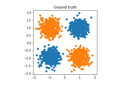
(a)

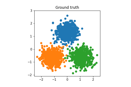
(b)

(c)

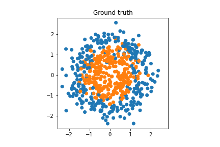
(d)

(e)

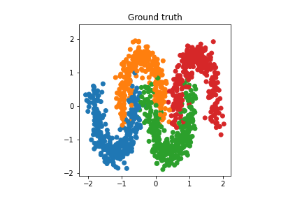
(f)

Figure 4: Training sample distributions of 2D examples: (a) Example 1: XOR, (b) Example 2: 3-Gaussian-blobs, (c) Example 3: 9-Gaussian-blobs, (d) Example 4: circle-and-ring, (e) Example 5: 2-new-moons and (f) Example 6: 4-new-moons, where different classes are in different colors.

Example 2 (3-Gaussian-blobs). There are three Gaussian-distributed classes in blue, orange and green as shown in Fig. 4(b). The three Gaussian blobs have identical covariance matrices. We use three lines and $D_{1}=6$ neurons in layer $l_{1}$ to separate them in Stage 1. Fig. 5(a) shows neuron responses in layer $l_{1}$. We see three neuron pairs: 0 and 3, 1 and 4, and 2 and 5. In Stage 2, we would like to isolate each Gaussian blob in a certain subspace. However, due to the shape of activated regions in Fig. 5(b), we need two neurons to preserve one Gaussian blob in layer $l_{2}$. For example, neurons 0 and 1 can preserve the Gaussian blob in the top as shown in Fig. 5(b).

If three partitioning lines $h_{1}$, $h_{2}$, $h_{3}$ intersect at nearly the same point as illustrated in Fig. 8(a), we have 6 nonempty regions instead of 7. Our FF-MLP design has $D_{in}=2$, $D_{1}=6$, $D_{2}=6$ and $D_{out}=3$. The training accuracy and the testing accuracy of the designed FF-MLP are 99.67% and 99.33%, respectively. This shows that the MLP splits the training data almost perfectly and fits the underlying data distribution very well.

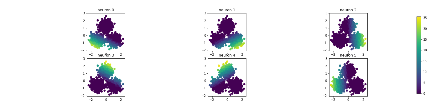
(a) 1st intermediate layer

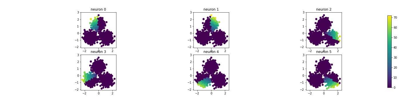
(b) 2nd intermediate layer

Figure 5: Response heatmaps for 3 Gaussian blobs in Example 2 in (a) layer $l_{1}$ and (b) layer $l_{2}$.

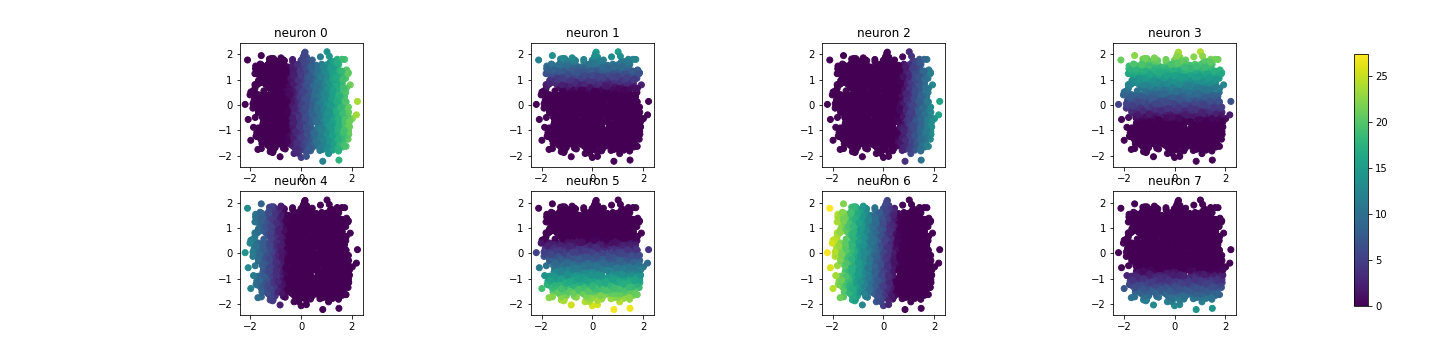
(a)

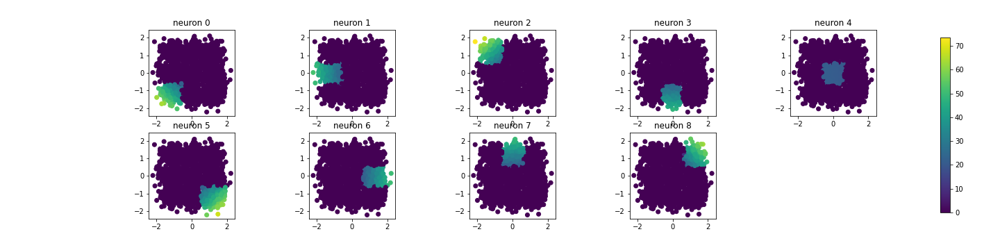
(b)

Figure 6: Neuron responses of the 9-Gaussian-blobs in Example 3 in (a) layer $l_{1}$ and (b) layer $l_{2}$.

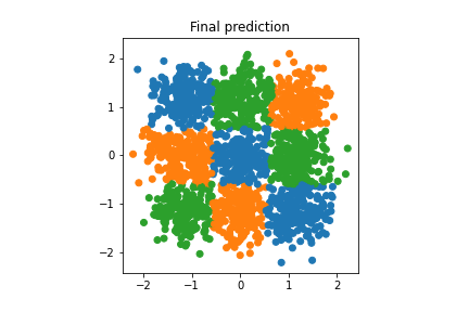
(a) Th=0.3

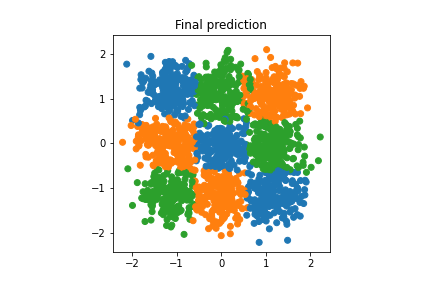
(b) Th=0.1

Figure 7: Comparison of classification results of FF-MLP for Example 3 with two different error thresholds: (a) Th=0.3 and (b) Th=0.1.

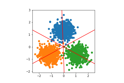
(a) Example 2

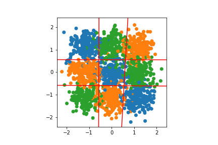
(b) Example 3

Figure 8: Partitioning lines for (a) Example 2 and (b) Example 3.

Example 3 (9-Gaussian-blobs). It contains 9 Gaussian blobs of the same covariance matrices aligned in 3 rows and 3 columns as shown in Fig. 4(c). In Stage 1, we need $C^{9}_{2}=36$ separating lines at most. We run the pruning algorithm with the error threshold equal to 0.3 and reduce the separating lines to 4, each of which partition adjacent rows and columns as expected. Then, there are $D_{1}=8$ neurons in layer $l_{1}$. The neuron responses in layer $l_{1}$ are shown in Fig. 6(a). They are grouped in four pairs: 0 and 4, 1 and 5, 2 and 6, and 3 and 7. In Stage 2, we form 9 regions, each of which contains one Gaussian blob as shown in Fig. 6(b). As shown in Fig. 8, we have two pairs of nearly parallel partitioning lines. Only 9 nonempty regions are formed in the finite range. The training and testing accuracy are 88.11% and 88.83% respectively. The error threshold affects the number of partitioning lines. When we set the error threshold to 0.1, we have 27 partitioning lines and $54$ neurons in layer $l_{1}$. By doing so, we preserve all needed boundaries between blobs of different classes. The training and testing accuracy are 89.11% and 88.58%, respectively. The performance difference is very small in this case.

(a)

(b)

Figure 9: Visualization of the 2-new-moons example: (a) the generated random samples from the fitted GMMs with 2 components per class and (b) the classification result of FF-MLP with error threshold equal to 0.1.

Figure 10: Classification results of FF-MLP for Example 6, where each new moon is approximated by 3 Gaussian components.

Example 4 (Circle-and-Ring). It contains an inner circle as one class and an outer ring as the other class as shown in Fig. 4(d)[9]. To apply our MLP design, we use one Gaussian blob to model the inner circle and approximate the outer ring with 4 and 16 Gaussian components, respectively. For the case of 4 Gaussian components, blobs of different classes can be separated by 4 partitioning lines. By using a larger number of blobs, we may obtain a better approximation to the original data. The corresponding classification results are shown in Figs. 12(a) and (b). We see that the decision boundary of 16 Gaussian components is smoother than that of 4 Gaussian components.

Example 5 (2-New-Moons). It contains two interleaving new moons as shown in Fig. 4(e)[9]. Each new moon corresponds to one class. We use 2 Gaussian components for each class and show the generated samples from the fitted GMMs in Fig. 9(a), which appears to be a good approximation to the original data visually. By applying our design to the Gaussian blobs, we obtain the classification result as shown in Fig. 9(b), which is very similar to the ground truth (see Table I).

Example 6 (4-New-Moons). It contains four interleaving new moons as shown in Fig. 4(f)[9], where each moon is a class. We set the number of blobs to 3 for each moon and the error threshold to 0.05. There are 9 partitioning lines and 18 neurons in layer $l_{1}$, which in turn yields 28 region neurons in layer $l_{2}$. The classification results are shown in Fig. 10. We can see that the predictions are similar to the ground truth and fit the underlying distribution quite well. The training accuracy is 95.75% and the testing accuracy is 95.38%.

V Observations on BP-MLP Behavior

Even when FF-MLP and BP-MLP adopt the same MLP architecture designed by our proposed method, BP-MLP has two differences from FF-MLP: 1) backpropagation (BP) optimization of the cross-entropy loss function and 2) network initialization. We report observations on the effects of BP and different initializations in Secs. V-A and V-B, respectively.

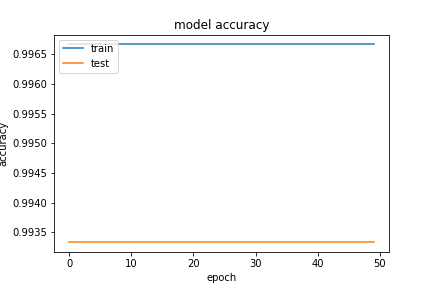
(a) 3-Gaussian-blobs

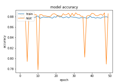
(b) 9-Gaussian-blobs, Th=0.3

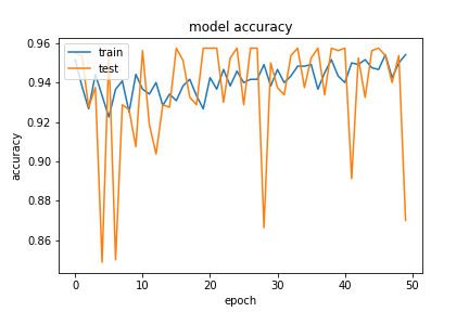
(c) 4-new-moons

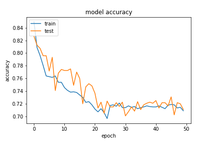
(d) 9-Gaussian-blobs, Th=0.1

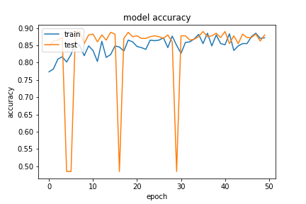
(e) circle-and-ring

Figure 11: Training and testing accuracy curves of BP-MLP as functions of the epoch number for (a) 3-Gaussian-blobs, (b) 9-Gaussian-blobs (Th=0.3), (c) 4-new-moons, (d) 9-Gaussian-blobs (Th=0.1) and (e) circle-and-ring, where the network is initialized by the proposed FF-MLP.

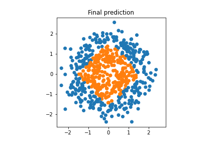
(a) FF-MLP, 4 Components

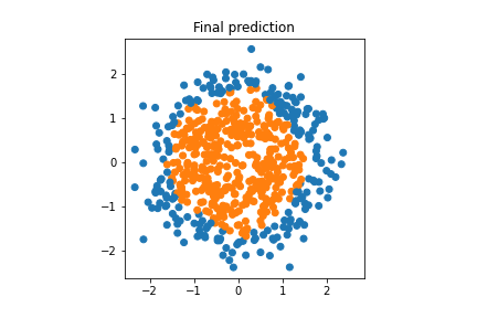
(b) FF-MLP, 16 Components

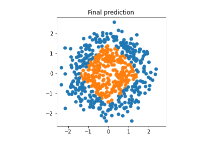
(c) BP-MLP, 4 Components

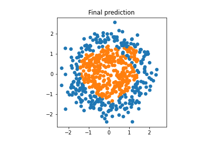
(d) BP-MLP, 16 Components

Figure 12: Classification results for the circle-and-ring example with (a) FF-MLP, 4 components, (b) FF-MLP, 16 components, (c) BP-MLP with FF-MLP initialization, 4 components, and (d) BP-MLP with FF-MLP initialization, 16 components.

V-A Effect of Backpropagation (BP)

We initialize a BP-MLP with weights and biases of the FF-MLP design and conduct BP using the gradient descent (SGD) optimizer with 0.01 learning rate and zero momentum. We observe four representative cases, and show the training and testing accuracy curves as a function of the epoch number in Figs. 11(a)-(e).

• BP has very little effect.
  One such example is the 3-Gaussian-blobs case. Both training and testing curves remain at the same level as shown in Fig. 11(a).

• BP has little effect on training but a negative effect on testing.
  The training and testing accuracy curves for the 9-Gaussian-blobs case are plotted as a function of the epoch number in Fig. 11(b). The network has 8 neurons in $l_{1}$ and 9 neurons in $l_{2}$, which is the same network architecture as in Fig. 7(a). Although the training accuracy remains at the same level, the testing accuracy fluctuates with several drastic drops. This behavior is difficult to explain, indicating the interpretability challenge of BP-MLP.

• BP has negative effects on both training and testing.
  The training and testing accuracy curves for 4-new-moons case are plotted as a function of the epoch number in Fig. 11(c). Both training and testing accuracy fluctuate and several drastic drops are observed for the testing accuracy. As shown in Table I, the final training and testing accuracy are lower compared to the FF-MLP results. The predictions for the training samples are shown in Fig. 14(a), which is worse than the ones in Fig. 10. Another example is the 9-Gaussian-blobs case with error threshold equal to 1. The training and testing accuracy decrease during training. The final training and testing accuracy are lower than FF-MLP as shown in Table I.

• BP has positive effect on both training and testing.
  For the circle-and-ring example when the outer ring is approximated with 16 components, the predictions for the training samples after BP are shown in Fig. 12(d). We can see the improvement in the training and testing accuracy in Table I. However, similar to the 9-Gaussian-blobs and 4-new-moons cases, we also observe the drastic drops of the testing accuracy during training.

V-B Effect of Initializations

We compare different initialization schemes for BP-MLP. One is to use FF-MLP and the other is to use the random initialization. We have the following observations.

• Either initialization works.
  For some datasets such as the 3-Gaussian-blob data, their final classification performance is similar using either random initialization or FF-MLP initialization.

• In favor of the FF-MLP initialization.
  We compare the BP-MLP classification results for 9-Gaussian-blobs with FF-MLP and random initializations in Fig. 13. The network has 8 neurons in $l_{1}$ and 9 neurons in $l_{2}$, which is the same network architecture as in Fig. 7(a). The advantage of the FF-MLP initialization is well preserved by BP-MLP. In contrast, with the random initialization, BP tends to find smooth boundaries to split data, which does not fit the underlying source data distribution in this case.

• Both initializations fail.
  We compare the BP-MLP classification results for 4-new-moons with FF-MLP and random initializations in Fig. 14. The result with the random initialization fails to capture the concave moon shape.

Generally speaking, BP-MLP with random initialization tends to over-simplify the boundaries and data distribution as observed in both 9-Gaussian-blobs and 4-new-moons.

(a) FF-MLP initialization

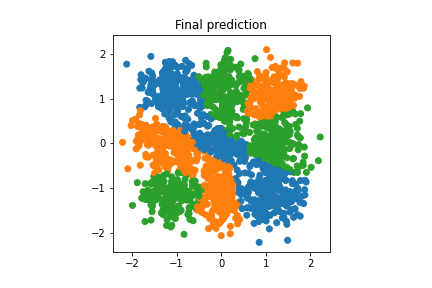
(b) random initialization

Figure 13: Comparison of BP-MLP classification results for 9-Gaussian-blobs with (a) FF-MLP initialization and (b) random initialization.

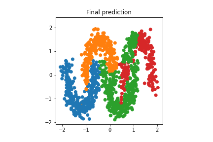
(a) FF-MLP initialization

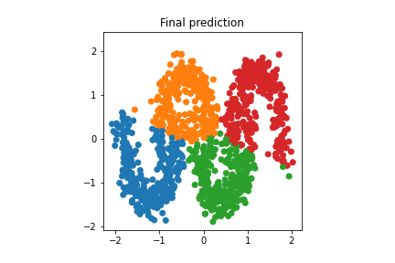
(b) random initialization

Figure 14: Comparison of BP-MLP classification results for 4-new-moons with (a) FF-MLP initialization and (b) random initialization.

VI Experiments

VI-A Classification Accuracy for 2D Samples

We compare training and testing classification performance among FF-MLP, BP-MLP with FF-MLP initialization, and BP-MLP with random initialization for Examples 1-6 in the last section in Table I. The integers in parentheses in the first row for BP-MLP are the epoch numbers. In the first column, the numbers in parentheses for the 9-Gaussian-blobs are error thresholds, the numbers in parentheses for the circle-and-ring are Gaussian component numbers for outer-ring’s approximations. For BP-MLP with random initialization, we report means and standard deviations of classification accuracy over 5 runs. We used the Xavier uniform initializer [13] for random initialization. We trained the network for two different epoch numbers; namely, 15 epochs and 50 epochs in different runs.

Dataset	FF-MLP		BP-MLP with FF-MLP init.(50)		BP-MLP with random init. (50)		BP-MLP with random init. (15)
	train	test	train	test	train	test	train	test
XOR	100.00	99.83	100.00	99.83	99.83 $\pm$ 0.16	99.42 $\pm$ 0.24	93.20 $\pm$ 11.05	92.90 $\pm$ 11.06
3-Gaussian-blobs	99.67	99.33	99.67	99.33	99.68 $\pm$ 0.06	99.38 $\pm$ 0.05	99.48 $\pm$ 0.30	99.17 $\pm$ 0.48
9-Gaussian-blobs (0.1)	89.11	88.58	70.89	71.08	84.68 $\pm$ 0.19	85.75 $\pm$ 0.24	78.71 $\pm$ 2.46	78.33 $\pm$ 3.14
9-Gaussian-blobs (0.3)	88.11	88.83	88.06	88.58	81.62 $\pm$ 6.14	81.35 $\pm$ 7.29	61.71 $\pm$ 9.40	61.12 $\pm$ 8.87
circle-and-ring (4)	88.83	87.25	89.00	86.50	81.93 $\pm$ 7.22	82.80 $\pm$ 5.27	70.57 $\pm$ 13.42	71.25 $\pm$ 11.27
circle-and-ring (16)	83.17	80.50	85.67	88.00	86.20 $\pm$ 1.41	85.05 $\pm$ 1.85	66.20 $\pm$ 9.33	65.30 $\pm$ 11.05
2-new-moons	88.17	91.25	88.17	91.25	83.97 $\pm$ 1.24	87.60 $\pm$ 0.52	82.10 $\pm$ 1.15	86.60 $\pm$ 0.58
4-new-moons	95.75	95.38	87.50	87.00	86.90 $\pm$ 0.25	84.00 $\pm$ 0.33	85.00 $\pm$ 0.98	82.37 $\pm$ 0.76

TABLE I: Comparison of training and testing classification performance between FF-MLP, BP-MLP with FF-MLP initialization and BP-MLP with random initialization. The best (mean) training and testing accuracy are highlighted in bold.

Let us focus on test accuracy. FF-MLP has better test performance with the following settings:

• XOR (99.83%)

• 9-Gaussian-blobs with error threshold 0.1 or 0.3 (88.58% and 88.83% respectively);

• circle-and-ring with 4 Gaussian components for the outer ring (87.25%);

• 2-new-moons (91.25%)

• 4-new-moons (95.38%).

Under these settings, FF-MLP outperforms BP-MLP with FF-MLP initialization or random initialization.

VI-B Classification Accuracy for Higher-Dimensional Samples

Besides 2D samples, we test FF-MLP for four higher-dimensional datasets. The datasets are described below.

• Iris Dataset. The Iris plants dataset [9, 14] is a classification dataset with 3 different classes and 150 samples in total. The input dimension is 4.

• Wine Dataset. The Wine recognition dataset [9, 15] has 3 classes with 59, 71, and 48 samples respectively. The input dimension is 13.

• B.C.W. Dataset. The breast cancer wisconsin (B.C.W) dataset [9, 15] is a binary classification dataset. It has 569 samples in total. The input dimension is 30.

• Pima Indians Diabetes Dataset. The Pima Indians diabetes dataset [16] is for diabetes prediction. It is a binary classification dataset with 768 8-dimensional entries. In our experiments, we removed the samples with the physically impossible value zero for glucose, diastolic blood pressure, triceps skin fold thickness, insulin, or BMI. We used only the remaining 392 samples.

We report the training and testing accuracy results of FF-MLP, BP-MLP with random initialization and trained with 15 and 50 epochs in Table II. For BP-MLP, the means of classification accuracy and the standard deviations over 5 runs are reported.

Dataset	$D_{in}$	$D_{out}$	$D_{1}$	$D_{2}$	Accuracy
					FF-MLP		BP-MLP/random init. (50)		BP-MLP/random init. (15)
					train	test	train	test	train	test
Iris	4	3	4	3	96.67	98.33	65.33 $\pm$ 23.82	64.67 $\pm$ 27.09	47.11 $\pm$ 27.08	48.33 $\pm$ 29.98
Wine	13	3	6	6	97.17	94.44	85.66 $\pm$ 4.08	79.72 $\pm$ 9.45	64.34 $\pm$ 7.29	61.39 $\pm$ 8.53
B.C.W	30	2	2	2	96.77	94.30	95.89 $\pm$ 0.85	97.02 $\pm$ 0.57	89.79 $\pm$ 2.41	91.49 $\pm$ 1.19
Pima	8	2	18	88	91.06	73.89	80.34 $\pm$ 1.74	75.54 $\pm$ 0.73	77.02 $\pm$ 2.89	73.76 $\pm$ 1.45

TABLE II: Training and testing accuracy results of FF-MLP and BP-MLP with random initialization for four higher-dimensional datasets. The best (mean) training and testing accuracy are highlighted in bold.

For the Iris dataset, we set the number of Gaussian components to 2 in each class. The error threshold is set to 0.05. There are 2 partitioning hyperplanes and, thus, 4 neurons in layer $l_{1}$. The testing accuracy for FF-MLP is 98.33%. For BP-MLP with random initialization trained for 50 epochs, the mean test accuracy is 64.67%. In this case, it seems that the network may have been too small for BP-MLP to arrive at a good solution.

For the wine dataset, we set the number of Gaussian components to 2 in each class. The error threshold is set to 0.05. There are 3 partitioning hyperplanes and thus 6 neurons in layer $l_{1}$. The testing accuracy for FF-MLP is 94.44%. Under the same architecture, BP-MLP with random initialization and 50 epochs gives the mean test accuracy of 79.72%. FF-MLP outperforms BP-MLP.

For the B.C.W. dataset, we set the number of Gaussian components to 2 per class. The error threshold is set to 0.05. There are 1 partitioning hyperplanes and thus 2 neurons in layer $l_{1}$. The testing accuracy for FF-MLP is 94.30%. The mean testing accuracy for BP-MLP is 97.02%. BP-MLP outperforms FF-MLP on this dataset.

Finally, for the Pima Indians dataset, we set the number of Gaussian components to 4 per class. The error threshold is set to 0.1. There are 9 partitioning hyperplanes and thus 18 neurons in layer $l_{1}$. The testing accuracy for FF-MLP is 73.89% while that for BP-MLP is 75.54% on average. BP-MLP outperforms FF-MLP in terms of testing accuracy.

VI-C Computational Complexity

We compare the computational complexity of FF-MLP and BP-MLP in Table III, Tesla V100-SXM2-16GB GPU was used in the experiments. For FF-MLP, we show the time of each step of our design and its sum in the total column. The steps include: 1) preprocessing with GMM approximation (stage 0), 2) fitting partitioning hyperplanes and redundant hyperplane deletion (stage 1), 3) Gaussian blob isolation (stage 2), and 4) assigning each isolated region to its corresponding output class (stage 3). For comparison, we show the training time of BP-MLP in 15 epochs and 50 epochs (in two separate runs) under the same network with random initialization.

Dataset	GMM	Boundary	Region	Classes	Total	BP (15)	BP (50)
		construction	representation	assignment
XOR	0.00000	0.01756	0.00093	0.00007	0.01855	2.88595 $\pm$ 0.06279	8.50156 $\pm$ 0.14128
3-Gaussian-blobs	0.00000	0.01119	0.00126	0.00008	0.01253	2.78903 $\pm$ 0.07796	8.26536 $\pm$ 0.17778
9-Gaussian-blobs (0.1)	0.00000	0.22982	0.00698	0.00066	0.23746	2.77764 $\pm$ 0.14215	8.34885 $\pm$ 0.28903
9-Gaussian-blobs (0.3)	0.00000	2.11159	0.00156	0.00010	2.11325	2.79140 $\pm$ 0.06179	8.51242 $\pm$ 0.24676
circle-and-ring (4)	0.02012	0.01202	0.00056	0.00006	0.03277	1.50861 $\pm$ 0.14825	3.79068 $\pm$ 0.28088
circle-and-ring (16)	0.04232	0.05182	0.00205	0.00020	0.09640	1.43951 $\pm$ 0.15573	3.80061 $\pm$ 0.13775
2-new-moons	0.01835	0.01111	0.00053	0.00006	0.03006	1.44454 $\pm$ 0.06723	3.64791 $\pm$ 0.08565
4-new-moons	0.03712	11.17161	0.00206	0.00021	11.21100	1.98338 $\pm$ 0.04357	5.71387 $\pm$ 0.14150
Iris	0.02112	0.02632	0.00011	0.00002	0.04757	0.73724 $\pm$ 0.01419	1.60543 $\pm$ 0.14658
Wine	0.01238	0.03551	0.00015	0.00003	0.04807	0.81173 $\pm$ 0.01280	1.72276 $\pm$ 0.07268
B.C.W	0.01701	0.03375	0.00026	0.00003	0.05106	1.08800 $\pm$ 0.05579	2.73232 $\pm$ 0.12023
Pima	0.03365	0.16127	0.00074	0.00039	0.19604	0.96707 $\pm$ 0.03306	2.32731 $\pm$ 0.10882

TABLE III: Comparison of computation time in seconds of FF-MLP (left) and BP-MLP (right) with 15 and 50 epochs. The mean and standard deviation of computation time in 5 runs are reported for BP-MLP. The shortest (mean) running time is highlighted in bold.

As shown in Table III FF-MLP takes 1 second or less in the network architecture and weight design. The only exceptions are 4-new-moons and 9-Gaussian-blobs with an error threshold of 0.3. Most computation time is spent on boundary construction, which includes hyperplane pruning. To determine the hyperplane to prune, we need to repeat the temporary hyperplane deletion and error rate computation for each hyperplane. This is a very time-consuming process. If we do not prune any hyperplane, the total computation time can be significantly shorter at the cost of a larger network size. Generally speaking, for non-Gaussian datasets, GMM approximation and fitting partitioning hyperplanes and redundant hyperplane deletion take most execution time among all steps. For datasets consisting of Gaussian blobs, no GMM approximation is needed. For BP-MLP, the time reported in Table III does not include network design time but only the training time with BP. It is apparent from the table that the running time in the FF-MLP design is generally shorter than that in the BP-MLP design.

VII Comments on Related Work

We would like to comment on prior work that has some connection with our current research.

VII-A BP-MLP Network Design

Design of the BP-MLP network architectures has been studied by quite a few researchers in the last three decades. It is worthwhile to review efforts in this area as a contrast of our FF-MLP design. Two approaches in the design of BP-MLPs will be examined in this and the next subsections: 1) viewing architecture design as an optimization problem and 2) adding neurons and/or layers as needed in the training process.

VII-A1 Architecture Design as an Optimization Problem

One straightforward idea to design the BP-MLP architecture is to try different sizes and select the one that gives the best performance. A good search algorithm is needed to reduce the trial number. For example, Doukim et al. [17] used a coarse-to-fine two-step search algorithm to determine the number of neurons in a hidden layer. First, a coarse search was performed to refine the search space. Then, a fine-scale sequential search was conducted near the optimum value obtained in the first step. Some methods were also proposed for both structure and weight optimization. Ludermir et al. [18] used a tabu search [19] and simulated annealing [20] based method to find the optimal architecture and parameters at the same time. Modified bat algorithm [21] was adopted in [22] to optimize the network parameters and architecture. The MLP network structure and its weights were optimized in [23] based on backpropagation, tabu search, heuristic simulated annealing, and genetic algorithms [24].

VII-A2 Constructive Neural Network Learning

In constructive design, neurons can be added to the network as needed to achieve better performance. Examples include: [25, 26, 27]. To construct networks, an iterative weight update approach [28] can be adopted [26, 27, 29, 30]. Neurons were sequentially added to separate multiple groups in one class from the other class in [31]. Samples of one class were separated from all samples of another class with a newly added neuron at each iteration. Newly separated samples are excluded from consideration in search of the next neuron. The input space is split into pure regions that contain only samples of the same class while the output of a hidden layer is proved to be linearly separable.

Another idea to construct networks is to leverage geometric properties [28], e.g., [32, 33, 34, 35, 36]. Spherical threshold neurons were used in [32]. Each neuron is activated if

$$\theta_{low}\leq d(\bm{W},\bm{X})\leq\theta_{high},$$ (8)

where $\bm{W}$, $\bm{X}$, $\theta_{low}$ and $\theta_{high}$ are the weight vector, the input vector, lower and higher thresholds respectively, and $d(\cdot)$ represents the distance function. That is, only samples between two spheres of radii $\theta_{low}$ and $\theta_{high}$ centered at the $\bm{W}$ are activated. At each iteration, a newly added neuron excludes the largest number of samples of the same class in the activated region from the working set. The hidden representations are linearly separable by assigning weights to the last layer properly. This method can determine the thresholds and weights without backpropagation.

VII-B Relationship with Work on Interpretation of Neurons as Partitioning Hyperplanes

The interpretation of neurons as partitioning hyperplanes was done by some researchers before. As described in Sec. VII-A2, Marchand et al. [31] added neurons to split the input space into pure regions containing only samples of the same class. Liou et al. [37] proposed a three-layer network. Neurons in the first layer represent cutting hyperplanes. Their outputs are represented as binary codes because of the use of threshold activation. Each region corresponds to a vertex of a multidimensional cube. Neurons in the second layer represent another set of hyperplanes cutting through the cube. They split the cube into multiple parts again. Each part may contain multiple vertices, corresponding to a set of regions in the input space. The output of the second layer is vertices in a multidimensional cube. The output layer offers another set of cuts. Vertices at the same side are assigned the same class, which implies the mergence of multiple regions. The weights and biases of links can be determined by BP. Neurons are added if the samples cannot be well differentiated based on the binary code at the layer output, which is done layer by layer. Cabrelli et al. [38] proposed a two-layer network for convex recursive deletion (CoRD) regions based on threshold activation. They also interpreted hidden layers as separating hyperplanes that split the input space into multiple regions. For each neuron, a region evaluates 0 or 1 depending on the side of the hyperplane that it lies in. Geometrically, the data points in each region lie in a vertex of a multidimensional cube. Their method does not require BP to update weights.

Results in [31, 37, 38] rely on threshold neurons. One clear drawback of threshold neurons is that they only have 0 or 1 binary outputs. A lot of information is lost if the input has a response range (rather than a binary value). FF-MLP uses the ReLU activation and continuous responses can be well preserved. Clearly, FF-MLP is much more general. Second, if a sample point is farther away from the boundary, its response is larger. We should pay attention to the side of the partitioning hyperplane a sample lies as well as the distance of a sample from the hyperplane. Generally, the response value carrys the information of the point position. This affects prediction confidence and accuracy. Preservation of continuous responses helps boost the classification accuracy.

We should point out one critical reason for the simplicity of the FF-MLP design. That is, we are not concerned with separating classes but Gaussian blobs in the first layer. Let us take the 9-Gaussian-blobs belonging to 3 classes as an example. There are actually $3^{9}$ ways to assign 9 Gaussian blobs to three classes. If we are concerned with class separation, it will be very complicated. Instead, we isolate each Gaussian blob through layers $l_{1}$ and $l_{2}$ and leave the blob-class association to the output layer. This strategy greatly simplifies our design.

VII-C Relationship with LDA and SVM

An LDA system can be viewed as a perceptron with specific weight and bias as explained in Sec. II. The main difference between an LDA system and a perceptron is the method to obtain their model parameters. While the model parameters of an LDA system are determined analytically from the training data distribution, the parameters of MLP are usually learned via BP.

There is a common ground between FF-MLP and the support-vector machine (SVM) classifier. That is, in its basic form, an SVM constructs the maximum-margin hyperplane to separate two classes, where the two-class LDA plays a role as well. Here, we would like to emphasize their differences.

• SVM contains only one-stage while FF-MLP contains multiple stages in cascade. Since there is no sign confusion problem with SVM, no ReLU activation is needed. For nonlinear SVM, nonlinearity comes from nonlinear kernels. It is essential for FF-MLP to have ReLU to filter out negative responses to avoid the sign confusion problem due to multi-stage cascade.

• The multi-class SVM is built upon the integration of multiple two-class SVMs. Thus, its complexity grows quickly with the number of underlying classes. In contrast, FF-MLP partitions Gaussian blobs using LDA in the first stage. FF-MLP connects each Gaussian blob to its own class type in Stage 3.

We can use a simple example to illustrate the second item. If there are $G$ Gaussian blobs belonging to $C$ classes, we have $C^{G}$ ways in definining the blob-class association. All of them can be easily solved by a single FF-MLP with slightly modification of the link weights in Stage 3. In contrast, each association demands one SVM solution. We need $C^{G}$ SVM solutions in total.

VII-D Relationship with Interpretable Feedforward CNN

Kuo et al. gave an interpretation to convolutional neural networks (CNNs) and proposed a feedforward design in [39], where all CNN parameters can be obtained in one-pass feedforward fashion without back-propagation. The convolutional layers of CNNs were interpreted as a sequence of spatial-spectral signal transforms. The Saak and the Saab transforms were introduced in [40] and [39], respectively, for this purpose. The fully-connected (FC) layers of CNNs were viewed as the cascade of multiple linear least squared regressors. The work of interpretable CNNs was built upon the mathematical foundation in [11, 41]. Recently, Kuo et al. developed new machine learning theory called “successive subspace learning (SSL)” and applied it to a few applications such as image classification [42] [43], 3D point cloud classification [44], [45], face gender classification [46], etc.

Although the FC layers of CNNs can be viewed as an MLP, we should point out one difference between CNN/FC layers and classical MLPs. The input to CNNs is raw data (e.g. images) or near-raw data (e.g., spectrogram in audio processing). Convolutional layers of CNNs play the role of feature extraction. The output from the last convolutional layer is a high-dimensional feature vector and it serves as the input to FC layers for decision. Typically, the neuron numbers in FC layers are monotonically decreasing. In contrast, the input to classical MLPs is a feature vector of lower dimension. The neuron number of intermediate layers may go up and down. It is not as regular as the CNN/FC layers.

VIII Conclusion and Future Work

We made an explicit connection between the two-class LDA and the MLP design and proposed a general MLP architecture that contains two intermediate layers, denoted by $l_{1}$ and $l_{2}$, in this work. The design consists of three stages: 1) stage 1: from input layer $l_{in}$ to $l_{1}$, 2) stage 2: from intermediate layer $l_{1}$ to $l_{2}$, 3) stage 3: from intermediate layer $l_{2}$ to $l_{out}$. The purpose of stage 1 is to partition the whole input space flexibly into a few half-subspace pairs. The intersection of these half-subspaces yields many regions of interest. The objective of stage 2 is to isolate each region of interest from other regions of the input space. Finally, we connect each region of interest to its associated class based on training data. We use Gaussian blobs to illustrate regions of interest with simple examples. In practice, we can leverage GMM to approximate datasets of general shapes. The proposed MLP design can determine the MLP architecture (i.e. the number of neurons in layers $l_{1}$ to $l_{2}$) and weights of all links in a feedforward one-pass manner without any trial and error. Experiments were conducted extensively to compare the performance of FF-MLP and the traditional BP-MLP.

There are several possible research directions for future extension. First, it is worthwhile to develop a systematic pruning algorithm so as to reduce the number of partitioning hyperplanes in stage 1. Our current pruning method is a greedy search algorithm, where the one that has the least impact on the classification performance is deleted first. It does not guarantee the global optimality. Second, it is well known that BP-MLP is vulnerable to adversarial attacks. It is important to check whether FF-MLP encounters the same problem. Third, we did not observe any advantage of using the backpropagation optimization in the designed FF-MLP in Sec. VI. One conjecture is that the size of the proposed FF-MLP is too compact. The BP may help if the network size is larger. This conjecture waits for further investigation. Fourth, for a general sample distribution, we approximate the distribution with Gaussian blobs that may have different covariances. This does not meet the homoscedasticity assumption of the two-class LDA. It is possible to improve the system by replacing LDA with heteroscedastic variants.

References

- [1] F. Rosenblatt, “The perceptron: a probabilistic model for information storage and organization in the brain.” Psychological review, vol. 65, no. 6, p. 386, 1958.
- [2] G. Cybenko, “Approximation by superpositions of a sigmoidal function,” Mathematics of control, signals and systems, vol. 2, no. 4, pp. 303–314, 1989.
- [3] K. Hornik, M. Stinchcombe, and H. White, “Multilayer feedforward networks are universal approximators,” Neural Networks, vol. 2, no. 5, pp. 359–366, 1989.
- [4] A. Ahad, A. Fayyaz, and T. Mehmood, “Speech recognition using multilayer perceptron,” in IEEE Students Conference, ISCON’02. Proceedings., vol. 1. IEEE, 2002, pp. 103–109.
- [5] A. V. Devadoss and T. A. A. Ligori, “Forecasting of stock prices using multi layer perceptron,” International Journal of Web Technology, vol. 2, no. 2, pp. 49–55, 2013.
- [6] K. Sivakumar and U. B. Desai, “Image restoration using a multilayer perceptron with a multilevel sigmoidal function,” IEEE transactions on signal processing, vol. 41, no. 5, pp. 2018–2022, 1993.
- [7] Z. Lu, H. Pu, F. Wang, Z. Hu, and L. Wang, “The expressive power of neural networks: A view from the width,” in Advances in neural information processing systems, 2017, pp. 6231–6239.
- [8] B. C. Csáji et al., “Approximation with artificial neural networks.”
- [9] F. Pedregosa, G. Varoquaux, A. Gramfort, V. Michel, B. Thirion, O. Grisel, M. Blondel, P. Prettenhofer, R. Weiss, V. Dubourg, J. Vanderplas, A. Passos, D. Cournapeau, M. Brucher, M. Perrot, and E. Duchesnay, “Scikit-learn: Machine learning in Python,” Journal of Machine Learning Research, vol. 12, pp. 2825–2830, 2011.
- [10] T. Hastie, R. Tibshirani, and J. Friedman, The elements of statistical learning, 2nd ed. Springer, 2017.
- [11] C.-C. J. Kuo, “Understanding convolutional neural networks with a mathematical model,” Journal of Visual Communication and Image Representation, vol. 41, pp. 406–413, 2016.
- [12] K. S. Gyamfi, J. Brusey, A. Hunt, and E. Gaura, “Linear classifier design under heteroscedasticity in linear discriminant analysis,” Expert Systems with Applications, vol. 79, pp. 44 – 52, 2017. [Online]. Available: http://www.sciencedirect.com/science/article/pii/S0957417417301306
- [13] X. Glorot and Y. Bengio, “Understanding the difficulty of training deep feedforward neural networks,” in Proceedings of the thirteenth international conference on artificial intelligence and statistics, 2010, pp. 249–256.
- [14] R. A. Fisher, “The use of multiple measurements in taxonomic problems,” Annals of eugenics, vol. 7, no. 2, pp. 179–188, 1936.
- [15] D. Dua and C. Graff, “UCI machine learning repository,” 2017. [Online]. Available: http://archive.ics.uci.edu/ml
- [16] J. W. Smith, J. Everhart, W. Dickson, W. Knowler, and R. Johannes, “Using the adap learning algorithm to forecast the onset of diabetes mellitus,” in Proceedings of the Annual Symposium on Computer Application in Medical Care. American Medical Informatics Association, 1988, p. 261.
- [17] C. A. Doukim, J. A. Dargham, and A. Chekima, “Finding the number of hidden neurons for an mlp neural network using coarse to fine search technique,” in 10th International Conference on Information Science, Signal Processing and their Applications (ISSPA 2010). IEEE, 2010, pp. 606–609.
- [18] T. B. Ludermir, A. Yamazaki, and C. Zanchettin, “An optimization methodology for neural network weights and architectures,” IEEE Transactions on Neural Networks, vol. 17, no. 6, pp. 1452–1459, 2006.
- [19] F. Glover, “Future paths for integer programming and links to artificial intelligence,” Computers & Operations Research, vol. 13, no. 5, pp. 533–549, 1986.
- [20] S. Kirkpatrick, C. D. Gelatt, and M. P. Vecchi, “Optimization by simulated annealing,” science, vol. 220, no. 4598, pp. 671–680, 1983.
- [21] X.-S. Yang, “A new metaheuristic bat-inspired algorithm,” in Nature inspired cooperative strategies for optimization (NICSO 2010). Springer, 2010, pp. 65–74.
- [22] N. S. Jaddi, S. Abdullah, and A. R. Hamdan, “Optimization of neural network model using modified bat-inspired algorithm,” Applied Soft Computing, vol. 37, pp. 71–86, 2015.
- [23] C. Zanchettin, T. B. Ludermir, and L. M. Almeida, “Hybrid training method for mlp: optimization of architecture and training,” IEEE Transactions on Systems, Man, and Cybernetics, Part B (Cybernetics), vol. 41, no. 4, pp. 1097–1109, 2011.
- [24] D. E. Goldberg, Genetic Algorithms in Search, Optimization and Machine Learning, 1st ed. USA: Addison-Wesley Longman Publishing Co., Inc., 1989.
- [25] R. G. Parekh, J. Yang, and V. Honavar, “Constructive neural network learning algorithms for multi-category real-valued pattern classification,” 1997.
- [26] M. Mezard and J.-P. Nadal, “Learning in feedforward layered networks: The tiling algorithm,” Journal of Physics A: Mathematical and General, vol. 22, no. 12, p. 2191, 1989.
- [27] M. Frean, “The upstart algorithm: A method for constructing and training feedforward neural networks,” Neural computation, vol. 2, no. 2, pp. 198–209, 1990.
- [28] R. Parekh, J. Yang, and V. Honavar, “Constructive neural-network learning algorithms for pattern classification,” IEEE Transactions on neural networks, vol. 11, no. 2, pp. 436–451, 2000.
- [29] I. Stephen, “Perceptron-based learning algorithms,” IEEE Transactions on neural networks, vol. 50, no. 2, p. 179, 1990.
- [30] F. F. Mascioli and G. Martinelli, “A constructive algorithm for binary neural networks: The oil-spot algorithm,” IEEE Transactions on Neural Networks, vol. 6, no. 3, pp. 794–797, 1995.
- [31] M. Marchand, M. Golea, and P. Ruján, “A convergence theorem for sequential learning in two-layer perceptrons,” EPL (Europhysics Letters), vol. 11, no. 6, p. 487, 1990.
- [32] J. Yang, R. Parekh, and V. Honavar, “Distal: An inter-pattern distance-based constructive learning algorithm,” Intelligent Data Analysis, vol. 3, no. 1, pp. 55–73, 1999.
- [33] E. Alpaydin, “Gal: Networks that grow when they learn and shrink when they forget,” International journal of pattern recognition and Artificial Intelligence, vol. 8, no. 01, pp. 391–414, 1994.
- [34] M. Marchand, “Learning by minimizing resources in neural networks,” Complex Systems, vol. 3, pp. 229–241, 1989.
- [35] N. K. Bose and A. K. Garga, “Neural network design using voronoi diagrams,” IEEE Transactions on Neural Networks, vol. 4, no. 5, pp. 778–787, 1993.
- [36] K. P. Bennett and O. L. Mangasarian, “Neural network training via linear programming,” University of Wisconsin-Madison Department of Computer Sciences, Tech. Rep., 1990.
- [37] C.-Y. Liou and W.-J. Yu, “Ambiguous binary representation in multilayer neural networks,” in Proceedings of ICNN’95-International Conference on Neural Networks, vol. 1. IEEE, pp. 379–384.
- [38] C. Cabrelli, U. Molter, and R. Shonkwiler, “A constructive algorithm to solve” convex recursive deletion”(cord) classification problems via two-layer perceptron networks,” IEEE Transactions on Neural Networks, vol. 11, no. 3, pp. 811–816, 2000.
- [39] C.-C. J. Kuo, M. Zhang, S. Li, J. Duan, and Y. Chen, “Interpretable convolutional neural networks via feedforward design,” Journal of Visual Communication and Image Representation, vol. 60, pp. 346–359, 2019.
- [40] C.-C. J. Kuo and Y. Chen, “On data-driven saak transform,” Journal of Visual Communication and Image Representation, vol. 50, pp. 237–246, 2018.
- [41] C.-C. J. Kuo, “The cnn as a guided multilayer recos transform [lecture notes],” IEEE signal processing magazine, vol. 34, no. 3, pp. 81–89, 2017.
- [42] Y. Chen and C.-C. J. Kuo, “Pixelhop: A successive subspace learning (ssl) method for object recognition,” Journal of Visual Communication and Image Representation, p. 102749, 2020.
- [43] Y. Chen, M. Rouhsedaghat, S. You, R. Rao, and C.-C. J. Kuo, “Pixelhop++: A small successive-subspace-learning-based (ssl-based) model for image classification,” arXiv preprint arXiv:2002.03141, 2020.
- [44] M. Zhang, H. You, P. Kadam, S. Liu, and C.-C. J. Kuo, “Pointhop: An explainable machine learning method for point cloud classification,” IEEE Transactions on Multimedia, 2020.
- [45] M. Zhang, Y. Wang, P. Kadam, S. Liu, and C.-C. J. Kuo, “Pointhop++: A lightweight learning model on point sets for 3d classification,” arXiv preprint arXiv:2002.03281, 2020.
- [46] M. Rouhsedaghat, Y. Wang, X. Ge, S. Hu, S. You, and C.-C. J. Kuo, “Facehop: A light-weight low-resolution face gender classification method,” arXiv preprint arXiv:2007.09510, 2020.