A black-box adversarial attack for poisoning clustering

Abstract

Clustering algorithms play a fundamental role as tools in decision-making and sensible automation processes. Due to the widespread use of these applications, a robustness analysis of this family of algorithms against adversarial noise has become imperative. To the best of our knowledge, however, only a few works have currently addressed this problem. In an attempt to fill this gap, in this work, we propose a black-box adversarial attack for crafting adversarial samples to test the robustness of clustering algorithms. We formulate the problem as a constrained minimization program, general in its structure and customizable by the attacker according to her capability constraints. We do not assume any information about the internal structure of the victim clustering algorithm, and we allow the attacker to query it as a service only. In the absence of any derivative information, we perform the optimization with a custom approach inspired by the Abstract Genetic Algorithm (AGA). In the experimental part, we demonstrate the sensibility of different single and ensemble clustering algorithms against our crafted adversarial samples on different scenarios. Furthermore, we perform a comparison of our algorithm with a state-of-the-art approach showing that we are able to reach or even outperform its performance. Finally, to highlight the general nature of the generated noise, we show that our attacks are transferable even against supervised algorithms such as SVMs, random forests and neural networks.

1 Introduction

The state of the art in machine learning and computer vision has greatly improved over the course of the last decade, to the point that many algorithms are commonly used as effective aiding tools in security (spam/malware detection [1], face recognition [2]) or decision making (road-sign detection [3], cancer detection [4], financial sentiment analysis [5]) related tasks. The increasing pervasiveness of these applications in our everyday life poses an issue about the robustness of the employed algorithms against sophisticated forms of non-random noise.

Adversarial learning has emerged over the past few years as a line of research focused on studying and addressing the aforementioned robustness issue. Perhaps, the most important result in this field is the discovery of adversarial noise, a wisely crafted form of noise that, if applied to an input, does not affect human judgment but can significantly decrease the performance of the learning models [6, 7]. Adversarial noise has been applied with success to fool models used in security scenarios such as spam filtering [8, 9, 10] or malware detection [11], but also in broader scenarios such as image classification [12].

The vast majority of the works done so far in this field deals with supervised learning. However, its unsupervised counterpart is equally present in sensible applications, such as fraud detection, image segmentation, and market analysis, not to mention the plethora of security-based applications for detecting dangerous or illicit activities [13, 14, 15, 16, 17].

It follows that the robustness of unsupervised algorithms used by those applications is crucial to give credibility to the results provided. Among the unsupervised tasks, in this work, we focus our attention on instance clustering with feature and image data.

The majority of clustering algorithms are not differentiable, thus adversarial gradient-based approaches – widely used in supervised settings – are not directly applicable. Since, in general, the machine learning field is currently dominated by gradient-based methods, this may represent a possible reason for the limited interest in this field. Nonetheless, the problem has been addressed in a complete white-box setting in [18, 11, 19], where some gradient-free attack algorithms have been proposed. In these works, the authors usually leverage the internal behavior of the clustering methods under study to craft ad-hoc adversarial noise. To the best of our knowledge, little work has been done against black-box algorithms. The design of black-box adversarial attacks, not only can help in finding common weaknesses of clustering algorithms but can also pave the road towards general rules for the formulation of robust clustering algorithms. In this work, we propose an algorithm to craft adversarial examples in a gradient-free fashion, without knowing the identity of the target clustering method. We assume that the attacker can only perform queries to it. Furthermore, we argue that, due to its general nature, the noise generated by our adversarial algorithm can also be applied to fool effectively supervised methods.

The main contributions of our work are as follows: (a) We design a new black-box gradient-free optimization algorithm to fool data clustering algorithms, and provide convergence guarantees. (b) We propose a new objective function that takes into consideration the attacker’s capability constraints, motivating its suitability in this setting. (c) We perform experiments on three different datasets against different clustering methods, showing that our algorithm can significantly affect the clustering performance. (d) Following the work of [20], we perform a transferability analysis, showing that our crafted adversarial samples are suitable to fool supervised algorithms.

2 Related Work

Several works use clustering for extracting data patterns in a given dataset. For instance, the work of [21] proposed Malheur, a tool for behavioral malware detection that combines clustering and classification for detecting novel malware categories. [14] have proposed AnDarwin, a software for detecting plagiarism in Android applications. In this approach, clustering is used to handle large numbers of applications, unlike previous methods that compare apps pairwise. More recently, [22] have presented a tool for anomaly detection in networking by using a clustering algorithm. Despite the greater need to have robust clustering algorithms, only a few works address their security problems.

The first works on the analysis of adversarial manipulations against clustering algorithms were proposed in [18] and [23]. The authors observed that some samples could be misclustered by positioning them close to the original cluster boundary, so that a new fringe cluster is formed.

[11] provided a theoretical formulation for the adversarial clustering problem and proposed a perfect-knowledge attack to fool single-linkage hierarchical clustering. In particular, the authors defined two different attack strategies: poisoning and obfuscation. The former infects data to violate the system availability and deteriorate the clustering results. The latter taints a target set of samples to violate the system integrity. In our threat model, we share the same aims of the poisoning strategy; however, differently from what has been done in [11], we extend the application of poisoning by allowing the attacker to manipulate already existing samples in the dataset instead of injecting new ones. Later on, in [24], the previous work was extended by proposing a threat model against complete-linkage hierarchical clustering. [19] defined a threat algorithm to fool DBSCAN-based algorithms by selecting and then merging arbitrary clusters.

All the aforementioned works assume that the attacker has perfect knowledge about the clustering algorithm under attack. In our work, we overcome this assumption by proposing a gradient-free algorithm to fool clustering algorithms in a generalized black-box setting, meaning that the attacker has no prior knowledge about the clustering algorithm and its parameters. We design our algorithm as an instance of an Abstract Genetic Algorithm [25], in which the adversarial noise improves generation by generation.

Recently, a similar problem has been addressed in [26], where it has been proposed a derivative-free, black-box attack strategy to target clustering algorithms working on linearly separable tasks. The approach consists of manipulating only one specific input sample feature-by-feature to corrupt the clustering decision boundary. However, our method is still different, since:

• It has been designed for attacking generic clustering algorithms (not only linearly separable ones).

• We propose a way to address multi-clustering problems by allowing the attacker to manipulate samples coming from different clusters.

• We prove that our algorithm has significant convergence properties to find the optimal perturbation for multiple samples and features at the same time.

• We penalize our solutions by considering the number of manipulated features in addition to the maximum acceptable noise threshold.

3 Methodology

Let $\boldsymbol{\mathbf{X}}\in\mathbb{R}^{n\times d}$ denote a feature matrix representing the dataset to be poisoned, where $n$ is the number of samples and $d$ is the number of features. We define $\mathcal{C}:\mathbb{R}^{n\times d}\rightarrow\{1,\dots,K\}^{n}$ to be the target clustering algorithm, that separates $n$ samples into $K$ different classes ($1\leq K\leq n$). We remark that by querying the clustering algorithm, the attacker can retrieve the number of clusters, and they may also change during the evaluation.

We consider the problem of crafting an adversarial mask $\boldsymbol{\mathbf{\epsilon}}$, to be injected into $\boldsymbol{\mathbf{X}}$, such that the clustering partitions $\mathcal{C}(\boldsymbol{\mathbf{X}})$ and $\mathcal{C}(\boldsymbol{\mathbf{X}}+\boldsymbol{\mathbf{\epsilon}})$ are different to a certain degree. In real scenarios, the attacker may follow some policies on the nature of the attack, usually imposed by intrinsic constraints on the problem at hand [27]. We model the scenario in which the attacker may want to perturb a specific subset of samples $T\subseteq\{1,\dots,n\}$, in such a way that the attack is less human-detectable. i.e. by constraining the norm of $\boldsymbol{\mathbf{\epsilon}}$ [28, 29]. In our work, the attacker’s capability constraints [27] are thus defined by (a) an attacker’s maximum power $\delta$, which is the maximum amount of noise allowed to be injected in a single entry $\boldsymbol{\mathbf{x}}_{ij}$, (b) an attacker’s maximum effort $\gamma$, which is the maximum number of manipulable entries of $\boldsymbol{\mathbf{X}}$. Further, we assume the attacker has access to the feature matrix $\boldsymbol{\mathbf{X}}$, and she can query the clustering algorithm $\mathcal{C}$ under attack. Similarly to [26] the adversary exercises a causative influence by manipulating part of the data to be clustered without any further information about the victim’s algorithm $\mathcal{C}$.

Given these considerations, an optimization program for our task is proposed as follows: —s— ϵ ∈E_T,δϕ(C(X), C(X + ϵ)) where $\phi$ is a similarity measure between clusterings, and

$$~{}\mathcal{E}_{T,\delta}=\{\boldsymbol{\mathbf{v}}\in\mathbb{R}^{n\times d},\|\boldsymbol{\mathbf{v}}\|_{\infty}<\delta\land\boldsymbol{\mathbf{v}}_{i}=\boldsymbol{\mathbf{0}}\ \forall i\notin T\}$$ (1)

is the adversarial attack space, which defines the space of all possible adversarial masks that satisfy the maximum power constraints and perturb only the samples in $T$. A problem without such capability constraints can be denoted with $\mathcal{E}_{\boldsymbol{\mathbf{X}},\infty}$. Note that $\gamma$ is not directly referenced in $\mathcal{E}_{T,\delta}$ but is bounded by $T$ itself, namely $\gamma=|T|\cdot d$.

We further elaborate Program 3 by searching for low Power & Effort (P&E) noise masks, in order to enforce the non-detectability of the attack. To this end, we adopt a similar strategy as in [30], which adds a penalty term $\lambda\|\boldsymbol{\mathbf{\epsilon}}\|_{p}$ to the cost function, usually with $p=0,2$ or $\infty$. Following this approach, we reformulate Program 3 by including a penalty term that takes into consideration both the attacker’s P&E which leverages the $\infty$ and $0$ norms, respectively. The optimization program becomes: —s— ϵ ∈E_T,δϕ(C(X), C(X + ϵ)) + λ∥ϵ∥_0 ∥ϵ∥_∞ This choice keeps the optimization program interpretable since it establishes a straightforward connection to our minimization desiderata (low P&E). In addition, our penalty term can be seen as a proxy function for $\|\boldsymbol{\mathbf{\epsilon}}\|_{p}$, granting similar regularization properties to the optimization. Indeed the P&E penalty is an upper bound to the single norm term, as the following lemma shows:

Lemma 1.

Let $\boldsymbol{\mathbf{x}}\in\mathbb{R}^{n}$, and $p,q\in\mathbb{R}\cup\{+\infty\}$ such that $1\leq p\leq q<+\infty$ then:

$$\|\boldsymbol{\mathbf{x}}\|_{p}\leq\|\boldsymbol{\mathbf{x}}\|_{0}\|\boldsymbol{\mathbf{x}}\|_{q}$$ (2)

Proof.

The case $\boldsymbol{\mathbf{x}}=\boldsymbol{\mathbf{0}}$ is trivial. Suppose that $\forall i$, $x_{i}\neq 0$, then for a known result on the equivalence of norms in $\mathbb{R}^{n}$ [31] we know that $\|\boldsymbol{\mathbf{x}}\|_{p}\leq n^{(1/p-1/q)}\|\boldsymbol{\mathbf{x}}\|_{q}$, thus:

$$\|\boldsymbol{\mathbf{x}}\|_{p} \leq n^{(1/p-1/q)}\|\boldsymbol{\mathbf{x}}\|_{q}\leq n^{1/p}\|\boldsymbol{\mathbf{x}}\|_{q}\leq n\|\boldsymbol{\mathbf{x}}\|_{q}$$

$$=\|\boldsymbol{\mathbf{x}}\|_{0}\|\boldsymbol{\mathbf{x}}\|_{q}$$ (3)

Suppose now, without loss of generality that $\boldsymbol{\mathbf{x}}=(x_{1},\dots,x_{m},0,\dots,0)^{\top}$, such that $\forall i\in\{1,\dots,m\}$, $x_{i}\neq 0$ . Consider its projection $\boldsymbol{\mathbf{x}}^{\prime}$ onto the axes $1,\dots,m$, then $\forall p\geq 0$, $\|\boldsymbol{\mathbf{x}}\|_{p}=\|\boldsymbol{\mathbf{x}}^{\prime}\|_{p}$. Thus Equation 3 holds since:

$$\|\boldsymbol{\mathbf{x}}\|_{p}=\|\boldsymbol{\mathbf{x}}^{\prime}\|_{p}\leq m\|\boldsymbol{\mathbf{x}}^{\prime}\|_{q}=\|\boldsymbol{\mathbf{x}}\|_{0}\|\boldsymbol{\mathbf{x}}\|_{q}$$

∎

3.1 Threat Algorithm

The approach we used to optimize Program (3), takes its inspiration from Genetic Algorithms (GA) [32]. These methods nicely fit our black-box setting since they do not require any particular property on the function to be optimized. Furthermore, our algorithm possesses solid convergence properties. In Section 3.3 we show that our algorithm is an instance of the Abstract Genetic Algorithm (AGA), as presented in [33, 25], and we give a proof of its convergence.

An additional constraint, usually imposed in real-world scenarios, is represented by the limited number of queries that can be performed to the algorithm under attack [34]. Classical approaches in GAs usually create large, fixed-size populations at each generation, and this, in turn, requires to compute the fitness score multiple times, querying $\mathcal{C}$ for each individual in the population, thereby making the process query-inefficient. To address this issue, we propose a growing size population approach. We start with a population $\Theta$ of size equal to $1$ and, generation by generation, we grow it by producing a new individual. To still harness the explorative power of GAs, we use a high mutation rate, and we allow the population set $\Theta$ to grow by keeping trace of all the previously computed individuals. In the case of memory-aware applications, our method can be extended by controlling the size of $\Theta$, in particular, by pruning low-fitness candidates. However, in our experiments, we adopted a different technique aimed to speed up the convergence of the optimization algorithm by reducing the number of generations (cf. Section 3.2).

Algorithm 1 Black-box poisoning

1:  Input: $\boldsymbol{\mathbf{X}}\in\mathbb{R}^{n\times d},\mathcal{C},\delta,T,G,l$

2:  Output: optimal adversarial mask $\boldsymbol{\mathbf{\epsilon}}^{*}$

3:  

4:  Initialize $\boldsymbol{\mathbf{\epsilon}}^{(0)}\in\mathcal{E}_{T,\delta}$ randomly

5:  $\Theta=\{\boldsymbol{\mathbf{\epsilon}}^{(0)}\}$

6:  

7:  for $g=0$ to $G-1$ do

8:     $\boldsymbol{\mathbf{\epsilon}}_{ch}^{(g+1)}=\texttt{choice}(\Theta,l)$

9:     $\boldsymbol{\mathbf{\epsilon}}_{cr}^{(g+1)}=\texttt{crossover}(\boldsymbol{\mathbf{\epsilon}}^{(g)},\boldsymbol{\mathbf{\epsilon}}_{ch}^{(g+1)})$

10:     $\boldsymbol{\mathbf{\epsilon}}^{(g+1)}=\texttt{mutation}(\boldsymbol{\mathbf{\epsilon}}_{cr}^{(g+1)},\delta,T)$

11:     $\Theta=\Theta\cup\{\boldsymbol{\mathbf{\epsilon}}^{(g+1)}\}$

12:  end for

13:  return: $\boldsymbol{\mathbf{\epsilon}}^{*}=\operatorname{arg\,min}_{\boldsymbol{\mathbf{\epsilon}}\in\Theta}l(\boldsymbol{\mathbf{\epsilon}})$

Algorithm 1 describes our optimization approach. It takes as input the feature matrix $\boldsymbol{\mathbf{X}}$, the clustering algorithm $\mathcal{C}$, the target samples $T$, the maximum attacker’s power $\delta$, the total number of generations $G$ (the attacker’s budget in term of queries) and the attacker’s objective function $l$ (which in our case is the one defined in Program (3)). The resulting output is the optimal adversarial noise mask $\boldsymbol{\mathbf{\epsilon}}^{*}$ that minimizes $l$. At each generation, a new adversarial mask $\boldsymbol{\mathbf{\epsilon}}^{(g+1)}$ is generated and added to a population set $\Theta$ containing all previous masks.

The core parts of our optimization process are the stochastic operators – choice, crossover and mutation – that we use for crafting new candidate solutions with a better fitness score. In the following, we describe their implementation.

Choice

The choice operator is used to decide which candidates will be chosen to generate offspring. We adopt a roulette wheel approach [32], where only one candidate is selected with a probability proportional to its fitness score, which in turn is inversely proportional to the attacker’s objective function $l$. Given a candidate $\boldsymbol{\mathbf{\epsilon}}^{(i)}$, its probability to be chosen for the production process $p(\boldsymbol{\mathbf{\epsilon}}^{(i)})$ is equal to:

$$p(\boldsymbol{\mathbf{\epsilon}}^{(i)})=\frac{\exp(-l(\boldsymbol{\mathbf{\epsilon}}^{(i)}))}{\sum_{\boldsymbol{\mathbf{\epsilon}}\in\Theta}\exp(-l(\boldsymbol{\mathbf{\epsilon}}))}$$ (4)

We remark that our choice operator picks just one adversarial noise mask that is then used in the crossover step.

Crossover

The crossover operator simulates the reproduction phase, by combining different candidate solutions (parents) for generating new ones (offspring). Commonly, crossover operators work with binary-valued strings, however, since our candidates are matrices in $\mathcal{E}_{T,\delta}$, we propose a variant. Given two candidates $\boldsymbol{\mathbf{\epsilon}}^{\prime},\boldsymbol{\mathbf{\epsilon}}^{\prime\prime}\in\mathcal{E}_{T,\delta}$, the new offspring is generated starting from $\boldsymbol{\mathbf{\epsilon}}^{\prime}$, then with probability equal to $p_{c}$ each entry $i,j$ is swapped with the entry $i,j$ in $\boldsymbol{\mathbf{\epsilon}}^{\prime\prime}$. The crossover operator has probability $p_{c}$ of being applied; in the case of failure, $\boldsymbol{\mathbf{\epsilon}}^{\prime}$ itself is chosen as an offspring.

Mutation

The mutation is a fundamental operator, usually applied to the offspring generated by the crossover, to introduce genetic variation in the current population. Our operator mutates each entry $\epsilon_{ij}$ s.t. $i\in T$ with probability $p_{m}$ by adding an uniformly distributed random noise in the range $[-\delta,\delta]$. The resulting perturbation matrix, is subsequently clipped to preserve the constraints dictated by $\mathcal{E}_{T,\delta}$.

Moreover, to enforce the low attacker’s effort desiderata, we also perform zero-mutation, meaning that each entry of the mask is set to zero with probability $p_{z}$.

Time complexity analysis

In this section we provide a time complexity analysis for Algorithm 1. In step 8, the objective function is computed, requiring, in turn, to execute the clustering algorithm $\mathcal{C}$ with complexity $O(\mathcal{C}(nd))$. Step 9 performs a cross-over between two adversarial masks, in $O(nd)$ time. The mutation of Step 10 is similarly computed in $O(nd)$ time. The overall time complexity is, thus, given by $O(G(\mathcal{C}(nd)+2nd))=O(G\mathcal{C}(nd))$, with G equal to the number of generations. The complexity of the clustering algorithm $\mathcal{C}(nd)$ is a key point in the efficiency of the attack. As an example, considering $K$-means, we have a polynomial-time of $O(G(ndKt+2n))=O(GndKt)$, with $K$ being the number of clusters and $t$ the number of iterations for the clustering algorithm.

3.2 Speeding up the convergence

By just generating a new individual at each generation, our proposed method has the major drawback of being slow at converging. To counter this problem, inspired by the work of [35], we decided to “imprint” a direction to the generated adversary mask to move the adversarial samples towards the target cluster. Since we lack the gradient information, the centroids information is leveraged instead. We propose the following approach: each adversarial mask $\boldsymbol{\mathbf{\epsilon}}\in\mathcal{E}_{T,\delta}$ is generated with the additional constraint that $\forall i,j$ $\epsilon_{ij}\geq 0$. After this, the mask is multiplied by a direction matrix $\boldsymbol{\mathbf{\psi}}$ with $\psi_{ij}=\operatorname{sgn}(c_{j}^{(t)}-c_{j}^{(v)})$, $\boldsymbol{\mathbf{c}}^{(t)}$ and $\boldsymbol{\mathbf{c}}^{(v)}$ being respectively the target and victim cluster centroids estimated from the victim data. The estimation is performed averaging the samples in the corresponding cluster. This variant can be easily implemented by changing the initialization of $\boldsymbol{\mathbf{\epsilon}}^{(0)}$ and the mutation step only. It follows that the resulting adversarial attack space is now reduced to $\mathcal{E}_{T,\delta}^{\prime}\subset\mathcal{E}_{T,\delta}$. We still grant that the capability constraints are respected and the convergence properties hold, although the quality of the found optimum may be inferior. In addition, we noticed that, without using this strategy, the optimization algorithm was more sensitive to the choice of hyper-parameters. Therefore, we have decided to adopt this strategy, which makes our algorithm more efficient and less sensitive to the choice of hyper-parameters.

3.3 Convergence properties

In general, GAs do not guarantee any convergence property [36]. However, under some more restrictive assumptions, it can be shown that they converge to an optimum. In this section, we show that our algorithm can be thought of as an instance of the Abstract Genetic Algorithm (AGA) as presented in [25, 33]. Subsequently, we give a proof of convergence. Below, we show the AGA pseudo-code:

Algorithm 2 Abstract Genetic Algorithm (pseudo-code)

1:  Make initial population

2:  

3:  while not stopping condition do

4:     Choose parents from population

5:     Let the selected parents Produce children

6:     Extend the population by adding the children to it

7:     Select elements of the extended population to survive for the next cycle

8:  end while

9:  Output the optimum of the population

In [25, 33], the authors show that methods such as classical Genetic Algorithms and Simulated Annealing can be thought of as instances of Algorithm 2. Further, they prove their probabilistic convergence to a (global) optimum. Following the same theoretical framework, we show that our algorithm indeed satisfies all the conditions for convergence. Before doing so, we first present the framework and adapt our algorithm in order to comply with it.

Let $S$ be a set of candidates and $S^{*}$ be a set of finite lists over $S$, representing all the possible finite populations. A neighborhood function is a function $N:S\rightarrow S^{*}$ that assigns neighbors to each individual in $S$. A parent-list, is a list of candidates able to generate offspring, with $P\subseteq S^{*}$ denoting the set of all parent-list. In our algorithm, a population is represented by a list $[\boldsymbol{\mathbf{\epsilon}}^{(0)},\dots,\boldsymbol{\mathbf{\epsilon}}^{(g)}]$, therefore $S=\mathcal{E}_{T,\delta}$, $S^{*}=\mathcal{E}_{T,\delta}^{*}$, $P=\{[\boldsymbol{\mathbf{\epsilon}}^{(i)},\boldsymbol{\mathbf{\epsilon}}^{(j)}]\mid\boldsymbol{\mathbf{\epsilon}}^{(i)},\boldsymbol{\mathbf{\epsilon}}^{(j)}\in\mathcal{E}_{T,\delta}\}$.

Let $f:X\rightarrow Y$ be a function belonging to $\mathcal{F}$, the set of all functions from $X$ to $Y$. Further, let $(\Omega,\mathcal{A},\mathbb{P})$ be a probability space and $g:\Omega\rightarrow\mathcal{F}$ be random variable. We define the randomized $f$ to be the function $f(\omega,x)=g(\omega)(x)$. Following this definition and [25], Algorithm 2 can be then detailed as follows:

Algorithm 3 Abstract Genetic Algorithm

1:  Create an $x\in S^{*}$

2:  

3:  while not stopping condition do

4:     draw $\alpha$, $\beta$ and $\gamma$

5:     $q=f_{c}(\alpha,x)$

6:     $y=\bigcup_{z\in q}f_{p}(\beta,z)$

7:     $x^{\prime}=x\cup y$

8:     $x=f_{s}(\gamma,x^{\prime})$

9:  end while

10:  output the actual population

with $f_{c}:A\times S^{*}\rightarrow\mathcal{P}(P)$ being the choice function, $f_{p}:B\times P\rightarrow\mathcal{P}(S)$ being the production function and $f_{s}:C\times S^{*}\rightarrow S^{*}$ being the selection function. In our case, we define:

1. $f_{c}(\alpha,x)=\{[\texttt{choice}(\alpha,x),x_{-1}]\},\ \forall\alpha\in A$

2. $f_{p}(\beta,[s_{1},s_{2}])=\texttt{mutation}(\beta,\texttt{crossover}(\beta,s_{1},s_{2}))),\ \forall\beta\in B$

3. $f_{s}(\gamma,x^{\prime})=x^{\prime}$ (Note that our selection is deterministic)

Where $x_{-1}$ is the most recent candidate in the population. In the above pseudo-code, we have explicitly stated the randomization of our procedures choice, mutation, crossover for clarity. The stochastic processes regulating the drawings of $\alpha$, $\beta$, and $\gamma$ always maintain the same distributions regardless of the current generation, meaning that the probability of generating a new population $x_{new}$ from another one $x_{old}$ does not change over the generations.

We now introduce and extend some definitions presented in [25]:

1. A neighborhood structure is connective if: $\forall s\in S,\forall t\in S:s\mapsto t$, where $\mapsto$ stands for the transitive closure of the relation $\{(s,t)\in S\times S\mid t\in N(s)\}$.

2. A choice function is generous if: (a) $\{[s,t]\mid s,t\in S\}\subseteq P$ and (b) $\forall x\in S^{*},\ \forall s_{1},s_{2}\in x:\mathbb{P}([s_{1},s_{2}]\in f_{c}(\alpha,x))>0$.

3. A production function is generous if: $\forall s_{1},s_{2}\in S,\ \forall t\in N(s_{1})\cup N(s_{2}):\mathbb{P}(t\in f_{p}(\beta,[s_{1},s_{2}]))>0$.

4. A selection function is generous if: $\forall x\in S^{*},\ \forall s\in x:\mathbb{P}(s\in f_{s}(\gamma,x))>0$.

5. A selection function is conservative if: $M_{x}\cap f_{s}(\gamma,x)\neq\emptyset$, with $M_{x}=\{s\in x\mid\forall t\in x:f(s)\leq f(t)\}$.

In [25] pag. 10, the authors further make a little technical assumption about the sets $A$, $B$, and $C$, requiring them to be countable, with positive probability for all their members. This is easily achieved in real applications considering the finiteness of the floating point representations.

Now we are ready to prove the following theorem:

Theorem 3.1.

Algorithm 3 almost surely reaches a global optimum.

Proof.

Given the previous considerations, the following statements hold:

1. Our neighborhood structure is connective: by the definition of our mutation operator, it holds that $N(\boldsymbol{\mathbf{\epsilon}}^{(i)})=\mathcal{E}_{T,\delta},\forall\boldsymbol{\mathbf{\epsilon}}^{(i)}\in\mathcal{E}_{T,\delta}$.

2. Our choice function is generous: this follows from (a) the definition of $P$, and from (b) the positivity of the softmax function in Equation 6.

3. Our production function is generous: See point 1.

4. Our selection function is generous: we allow all the candidates to survive with probability $1$.

5. Our selection function is conservative: see point 4.

The proof then follows from Theorem $3$ in [33], adjusting the generousness definitions with our versions presented above. The globality of the optimum comes from the fact that our algorithm performs a global search, instead of a local one. ∎

The same conclusions can be drawn for the speed-up heuristic, by just replacing each instance of $\mathcal{E}_{T,\delta}$, with $\mathcal{E}_{T,\delta}^{\prime}$.

4 Experimental results

In this section, we present an experimental evaluation of the proposed methodology of attack.

4.1 Robustness analysis

We ran the experiments on three real-world datasets: FashionMNIST [37], CIFAR-$10$ [38] and $20$ Newsgroups [39]. We focused our analysis on both two- and multiple-way clustering problems. For FashionMNIST and $20$ Newsgroups, we simulated the former scenario in which an attacker wants to perturb samples of one victim cluster $C_{v}$ towards a target cluster $C_{t}$. For CIFAR-$10$, we allowed the attacker to move samples from multiple victim clusters towards a target one by simply running multiple times our algorithm with a different victim cluster for each run. In the experiments, we chose $T$ to contain the $s|C_{v}|$ nearest neighbors belonging to the currently chosen victim cluster, with respect to the centroid of the target cluster. In particular, for FashionMNIST we used $20$ different values for $s$ and $\delta$, in the intervals $[0.01,0.6]$ and $[0.05,1]$ respectively; for CIFAR-$10$ we used $20$ different values for $s$ and $\delta$, in the intervals $[0.01,0.6]$ and $[0.01,1.5]$ respectively; for $20$ Newsgroups we used $15$ different values for $s$ and $\delta$, in the intervals $[0.01,0.3]$ and $[0.001,0.3]$ respectively.

We tested the robustness of three standard clustering algorithms: hierarchical clustering using Ward’s criterion [40], $K$-means++ [41] and the normalized spectral clustering [42] as presented in [43], with the [44] similarity measure. The code has been written in PyTorch [45] and it available at .

For the optimization program, we set $\lambda=\frac{1}{\alpha\cdot n\cdot d}$ with $\alpha=255$ as penalty term for our cost function. In addition, in the optimization algorithm, we set the probability of having crossover $p_{c}=0.85$, mutation $p_{m}=0.05$ and zero-mutation $p_{z}=0.001$. The total number of generations G, which correspond to the number of queries, was always set to $110$, using the heuristic proposed in Section 3.2. In addition, we repeated these experiments for five times, reporting the mean with the standard error.

In Program (3), we indicate with $\phi$ a function for measuring the similarity between two clustering partitions. In the literature, we can find several metrics used for the evaluation of clusterings [46, 47, 48, 49]; in addition, [11] proposed to adopt the following measure for the evaluation: $d(\boldsymbol{\mathbf{Y}},\boldsymbol{\mathbf{Y}}^{\prime})=\|\boldsymbol{\mathbf{Y}}\boldsymbol{\mathbf{Y}}^{\top}-\boldsymbol{\mathbf{Y}}^{\prime}{\boldsymbol{\mathbf{Y}}^{\prime}}^{\top}\|_{F}$, where $\|\cdot\|_{F}$ is the Frobenius norm, and $\boldsymbol{\mathbf{Y}},\boldsymbol{\mathbf{Y}}^{\prime}\in\mathbb{R}^{n\times k}$ are one-hot encodings of the clusterings $\mathcal{C}(\boldsymbol{\mathbf{X}})$ and $\mathcal{C}(\boldsymbol{\mathbf{X}}+\boldsymbol{\mathbf{\epsilon}})$ respectively. In our work, we decided to use the Adjusted Mutual Information (AMI) Score, proposed in [49] since it makes no assumptions about the cluster structure and, as highlighted in [50], it works well even in the presence of unbalanced clusters. Indeed, the clustering partition over the poisoned dataset might also create unbalanced clusters, especially if the attacker wants to move samples only from one towards the others.

The AMI score between two clustering partitions $U$ and $V$ is given by:

$$AMI(U,V)={\frac{MI(U,V)-\mathbb{E}[MI(U,V)]}{\max{\{H(U),H(V)\}}-\mathbb{E}[MI(U,V)]}}$$ (5)

where $MI(U,V)$ measures the mutual information shared by the two partitions, $\mathbb{E}[MI(U,V)]$ represents its expected mutual information and $\max{\{H(U),H(V)\}}$ is the maximum between the two entriopies, which is an upper bound for $MI(U,V)$. AMI is equal to $1$ when the two clustering partitions are identical, and $0$ when they are independent, that is, sharing no information about each other.

The reader can refer to Section 4.1.4 where a comparison analysis between different similarity functions is offered.

Figure 1: Robustness analysis with FashionMNIST (left), CIFAR-$10$ (middle), $20$ Newsgroups (right). The plots depict the decay of AMI by adversarially perturbing the datasets, with an increasing noise.

4.1.1 FashionMNIST

The FashionMNIST contains $70\,000$ grayscale images of size $28\times 28$ pixels [37]. In our experiments we randomly sampled $800$ images for class Ankle boot (victim cluster) and $800$ for class Shirt (target cluster). In Figure 1 (left), we report the obtained results. We observe that the three algorithms have similar behavior and their clustering accuracy consistently decreases with the increment of the adversarial noise level. In this case, $K$-means++ shows better performance than spectral clustering, therefore the spectral embedding of data samples seems less robust than raw features only. This fact may suggest that some embedding procedures devised for improving clustering accuracy do not necessarily guarantee robustness against adversarial attacks. However, we reserve further discussion on this in future work.

4.1.2 CIFAR-10

The CIFAR-$10$ contains $60\,000$ colour images of size $32\times 32$ pixels [38]. We randomly sampled $1\,600$ images from classes airplane, frog and automobile. We addressed the multi-way scenario by first moving samples from airplane and then from frog, always towards the target cluster automobile. Moreover, we used a ResNet50 for features extraction, and we performed clustering on the resulting feature space, obtaining better initial results in terms of AMI. In Figure 1 (middle), we show the performance of the three clustering algorithms under adversarial manipulations. We observe that our attacks significantly decrease the clustering quality for the three algorithms. Even if the ResNet50 features allow cluster algorithms to achieve better performance, they are still vulnerable to adversarial noise. Further, note how the gap in performance of spectral clustering and $K$-means++ has even increased when adopting a DNN-generated embedding.

We provide, in Figure 2, a visual representation of poisoning samples for CIFAR-10. We reconstructed the poisoning samples from the feature space using the feature collision strategy adopted in [51], where the target is exactly our poisoning sample.

4.1.3 20 Newsgroups

The $20$ Newsgroups is a dataset commonly used for text classification and clustering, which contains $20\,000$ newspaper articles divided into $20$ categories. The experiments were conducted with two highly unrelated categories of news, rec.sport.baseball (victim cluster) and talk.politics.guns (target cluster). We applied the a combination of TF-IDF [52] and LSA [53] to embed features into a lower dimensional space. The resulting feature matrix had dimension $1\,400\times 80$. In this case, we tested our method against two ensemble clustering algorithms, derived from $K$-means and spectral clustering algorithms (hierarchical clustering was not giving good enough clustering performance). The two algorithms use the Silhouette value [54], and the clustering with the maximum silhouette score is selected as the best one. In particular, we ran $20$ instances of the $K$-means algorithm with random centroids initializations, while, for spectral clustering, we ran $3$ instances of the algorithm proposed in [43] with $3$ different similarity measures. Given a sample pair $\boldsymbol{\mathbf{x}}_{i}$ and $\boldsymbol{\mathbf{x}}_{j}$, the measures are:

$$s_{ij} =\frac{\boldsymbol{\mathbf{x}}_{i}^{\top}\boldsymbol{\mathbf{x}}_{j}}{\|\boldsymbol{\mathbf{x}}_{i}\|_{2}\|\boldsymbol{\mathbf{x}}_{j}\|_{2}}$$ (6)

$$s_{ij} =\frac{(\boldsymbol{\mathbf{x}}_{i}-\bar{\boldsymbol{\mathbf{x}}})^{\top}(\boldsymbol{\mathbf{x}}_{j}-\bar{\boldsymbol{\mathbf{x}}})}{\|\boldsymbol{\mathbf{x}}_{i}-\bar{\boldsymbol{\mathbf{x}}}\|_{2}\|\boldsymbol{\mathbf{x}}_{j}-\bar{\boldsymbol{\mathbf{x}}}\|_{2}}$$ (7)

$$s_{ij} =d_{max}-\|\boldsymbol{\mathbf{x}}_{i}-\boldsymbol{\mathbf{x}}_{j}\|_{2}$$ (8)

Equation 6 represents the cosine similarity between two samples $\boldsymbol{\mathbf{x}}_{i}$ and $\boldsymbol{\mathbf{x}}_{j}$. Equation 7 is the Pearson correlation coefficient, with $\bar{\boldsymbol{\mathbf{x}}}$ being the sample mean. Moreover, we introduced a sparsification technique, clamping to $0$ all negative values, which improved the clustering performance. Finally, in Equation 8 we define $d_{max}=\max_{ij}\|\boldsymbol{\mathbf{x}}_{i}-\boldsymbol{\mathbf{x}}_{j}\|_{2}$.

Figure 1 (right) reports the performance of two clustering algorithms under adversarial manipulation. Ensemble methods are known to be more robust against random noise with respect to the normal behavior of the corresponding algorithms [55, 56]; however, our attacking model was able to fool them and significantly decreased their clustering performance. In this case, in low noise regime, spectral clustering seems to benefit the ensembling technique, however its behavior follows previous experiments.

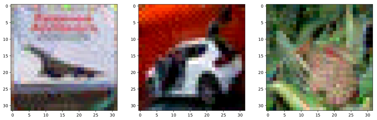
Figure 2: (Top row) clean samples from CIFAR-10. (Bottom row) the corresponding poisoning samples with $\delta$ = $0.1$.

4.1.4 Choice of the cost function

In our optimization program, we employed the AMI both for the cost function $\phi$ and the evaluation measure. Indeed, our optimization being not derivative-dependent, we could adopt the same function for the optimization and evaluation tasks.

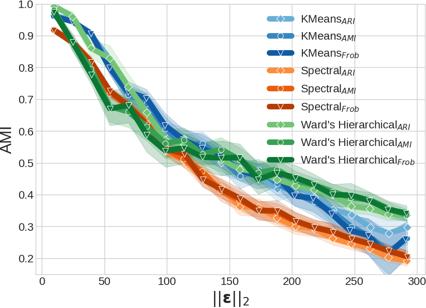
Figure 3: Robustness analysis on FashionMNIST by changing the similarity measure $\phi$ (left), and crafting the poisoning samples employing a surrogate dataset (right).

We decided to analyze the impact of the clustering similarity function $\phi$, with FashionMNIST, and see if there were significant differences among each other. In Figure 3 (left), shows the variation of results with $\phi$ equals to ARI [46], AMI [49] and the negated distance proposed in [11] (referred as “Frob”). The plot shows no substantial difference among the choices of $\phi$, suggesting that this hyperparameter does not significantly impact the optimization process.

4.1.5 Surrogate data

We ran additional experiments on a more challenging scenario by relaxing the knowledge assumption of the target data. In this scenario, the attacker does not have access to the target data and can only sample a surrogate dataset from the same distribution. To this end, we have randomly sampled two subsets of 1600 images, each extracted from FashionMNIST as detailed in Section 4.1.1. We use the first one to create the poisoning samples and then evaluate their effectiveness on the other one. Figure 3 (right) shows that our attack is strong enough to decrease the clustering performance even when the attacker has no access to the target dataset.

4.2 Comparison

To the best of our knowledge, the only work dealing with adversarial clustering in a black-box way is [26]. In this work, the authors presented a new type of attack called spill-over, in which the attacker wants to assign as many samples as possible to a wrong cluster by poisoning just one of them. They proposed a threat model against linearly separable clusters to generate such kind of adversarial noise.

Method	$\|\boldsymbol{\mathbf{\epsilon}}\|_{0}$	$\|\boldsymbol{\mathbf{\epsilon}}\|_{2}$	$\|\boldsymbol{\mathbf{\epsilon}}\|_{\infty}$	#Miss-clust
Spill-over	413	872.8	146.8	$2$
Spill-overclamp	412	828.2	146.8	$2$
Ours $(\delta=73.43)$	$151\pm 19.2$	$551.9\pm 36.3$	$73.4\pm 1.4$	$12.0\pm 0.0$
Ours $(\delta=146.87)$	$30\pm 7.6$	$479.1\pm 62.5$	$145.0\pm 3.7$	$12.0\pm 0.0$
Ours $(\delta=\infty)$	$29\pm 13.8$	$757.1\pm 203.2$	$246.25\pm 16.8$	$14.3\pm 2.4$

Table 1: Comparison on MNIST with digits 3&2.

Method	$\|\boldsymbol{\mathbf{\epsilon}}\|_{0}$	$\|\boldsymbol{\mathbf{\epsilon}}\|_{2}$	$\|\boldsymbol{\mathbf{\epsilon}}\|_{\infty}$	#Miss-clust
Spill-over	152	585.3	159.7	11
Spill-overclamp	151	463.2	131.7	9
Ours $(\delta=79.86)$	$117\pm 7.8$	$528.4\pm 30.1$	$79.8\pm 2.8$	$9.1\pm 0.4$
Ours $(\delta=159.72)$	$75\pm 22.4$	$782.7\pm 124.2$	$159.3\pm 1.3$	$12.0\pm 4.5$
Ours $(\delta=\infty)$	$46\pm 19.4$	$902.7\pm 205$	$248.3\pm 8.8$	$14.6\pm 4.5$

Table 2: Comparison on MNIST with digits 4&1.

To have a fair comparison, we performed spill-over attacks on the same settings of the aforementioned work, comparing the performance on MNIST and UCI Handwritten Digits datasets [57], targeting Ward’s hierarchical clustering algorithm. Further details can be found in Appendix.

For MNIST, we considered the digit pairs $4\&1$ and $3\&2$, while for Digits, we considered the digit pairs $4\&1$, and $8\&9$. Our algorithm was run with the $\delta=\Delta$ which is the maximum acceptable noise threshold found by the authors, with $\delta=\Delta/2$ and with $\delta=\infty$. We found the value of $\Delta$ used in [26] by looking at the source code. We imposed to attack just one sample ($|T|=1$), namely the nearest neighbor to the centroid of the target cluster. We performed our experiments $20$ times, reporting mean and std values.

Method	$\|\boldsymbol{\mathbf{\epsilon}}\|_{0}$	$\|\boldsymbol{\mathbf{\epsilon}}\|_{2}$	$\|\boldsymbol{\mathbf{\epsilon}}\|_{\infty}$	#Miss-clust
Spill-over	54	15.70	9.44	21
Spill-overclamp	54	15.70	9.44	21
Ours $(\delta=4.72)$	$12\pm 1.20$	$11.49\pm 1.25$	$4.7\pm 0$	$21\pm 0.0$
Ours $(\delta=9.44)$	$7\pm 2.85$	$13.86\pm 2.96$	$8.12\pm 1.24$	$21\pm 0.0$
Ours $(\delta=\infty)$	$4\pm 1.74$	$15.18\pm 3.16$	$10.94\pm 1.49$	$21\pm 0.0$

Table 3: Comparison on Digits with digits 8&9.

Method	$\|\boldsymbol{\mathbf{\epsilon}}\|_{0}$	$\|\boldsymbol{\mathbf{\epsilon}}\|_{2}$	$\|\boldsymbol{\mathbf{\epsilon}}\|_{\infty}$	#Miss-clust
Spill-over	14	23.93	11.89	24
Spill-overclamp	11	16.28	9.93	21
Ours $(\delta=5.94)$	$13\pm 1.70$	$16.27\pm 1.20$	$5.94\pm 0.0$	$24\pm 0.0$
Ours $(\delta=11.89)$	$7\pm 2.03$	$19.84\pm 1.96$	$11.13\pm 0.79$	$24\pm 0.0$
Ours $(\delta=\infty)$	$7\pm 2.36$	$21.06\pm 2.36$	$12.79\pm 4.34$	$24\pm 0.0$

Table 4: Comparison on Digits with digits 4&1.

The results are presented in Table 1-4 along with more details on the experiments. Although our algorithm achieves its best performance by moving more samples at once, we were able to match, or even exceed, the number of spill-over samples (#Miss-clust) achieved in [26], even when halving the attacker’s maximum power proposed by the authors. Moreover, the results show also that we were able to craft adversarial noise masks $\boldsymbol{\mathbf{\epsilon}}$, which were significantly less detectable in terms of $\ell_{0},\ell_{\infty}$.

In Table 5-6, we report a comparison for the $K$-means++ algorithm with UCI Wheat Seeds [58] and MoCap Hand Postures [59] dataset, repeating the same experimental setting of [26]. We obtain the same number of spill-over samples (#Miss-Clust) with significant lower Power & Effort.

Finally, in Figure 4 and 5, we show a qualitative assessment of the crafted adversarial spill-over samples. Note that the crafted adversarial examples of [26] do not preserve box-constraints commonly adopted for image data. Indeed, pixel intensities exceed $255$ and $16$ for MNIST and Digits, respectively. We also evaluated the performance of [26] by clamping the resulting adversarial examples (Spill-over_clamp), and we observe that the number of spill-over samples is reduced.

Method	$\|\boldsymbol{\mathbf{\epsilon}}\|_{0}$	$\|\boldsymbol{\mathbf{\epsilon}}\|_{2}$	$\|\boldsymbol{\mathbf{\epsilon}}\|_{\infty}$	#Miss-clust
Spill-over	7	0.42	0.30	$2$
Ours $(\delta=0.15)$	$3\pm 0.79$	$0.14\pm 0.04$	$0.10\pm 0.03$	$2.0\pm 0.0$
Ours $(\delta=0.30)$	$3\pm 0.76$	$0.28\pm 0.09$	$0.21\pm 0.06$	$2.0\pm 0.0$

Table 5: Comparison for Seeds.

Method	$\|\boldsymbol{\mathbf{\epsilon}}\|_{0}$	$\|\boldsymbol{\mathbf{\epsilon}}\|_{2}$	$\|\boldsymbol{\mathbf{\epsilon}}\|_{\infty}$	#Miss-clust
Spill-over	9	44.42	20.0	$5$
Ours $(\delta=10)$	$1\pm 0.48$	$5.13\pm 1.86$	$5.0\pm 1.86$	$5.0\pm 0.0$
Ours $(\delta=20)$	$1\pm 1.14$	$8.50\pm 6.61$	$7.74\pm 5.18$	$5.0\pm 0.0$

Table 6: Comparison for MoCap Hand Postures.

Figure 4: Spill-over samples for MNIST. The target sample (left), the corresponding adversarial sample crafted with the attack proposed in [26] (middle), and our adversarial sample with $\delta=146.87$

(right).

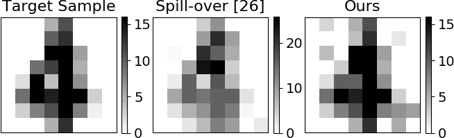
Figure 5: Spill-over samples for Digits. The target sample (left), the corresponding adversarial sample crafted with the attack proposed in [26] (middle), and our adversarial sample with $\delta=11.89$ (right).

In conclusion, [26] aims to find $\Delta$, which does not lead to the attack being considered an outlier using the , Coordinate-wise Min-Mahalanobis-Depth (COMD) measure, at the expense of existing box-constraints. Whereas our purpose consists of proposing an algorithm that can effectively corrupt a black-box clustering algorithm’s performance by minimizing the attacker’s power and effort (P&E). Indeed, our attacks, as shown in Table 3-6, show lower $\ell_{0}$ and $\ell_{\infty}$ compared to the attack obtained with [26]. These results suggest that our algorithm can craft effective poisoning attacks, even stronger than [26], with less P&E and satisfying the box-constraints

Ablation study

We provide an ablation study for the mutation and zero rate parameters, $p_{m}$ and $p_{z}$ respectively, keeping the crossover rate $p_{c}$ set to $0.85$ for the two pairs of MNIST digits. The high crossover rate is a common choice in Genetic Algorithms [60]. We use the same setting described in Section 4.2 with dataset MNIST 3&2 and MNIST 4&1.

Figure 6: Ablation study for mutation rate (x-axis) and zero rate (y-axis) for MNIST 3&2. (left) Number of miss clustered samples, (right) attacker’s effort, i.e., number of manipulated pixels.

Figure 7: Ablation study for mutation rate (x-axis) and zero rate (y-axis) for MNIST 4&1. (left) number of miss clustered samples, (right) attacker’s effort, i.e., number of manipulated pixels.

Fig. 6 and Fig. 7 reveal how the two hyperparameters affect the attacker’s effort and the strength of the attacks created. An increment of the zero rate implies attacks with less effort, while an increment of the mutation inverts this tendency thus generating more powerful attacks. From Figure 6-7 (left), we observe that the yellow regions at the bottom left determine a good compromise on having a small effort and good attack effectiveness. However, by increasing the attacker’s effort, we can generate even more effective attacks. The results of the ablation study with the two pairs of digits are similar, suggesting that the same set of hyperparameters can be chosen without significant differences, as also suggested by the wide bottom-left regions of Figure 6-7 (left) where the number of miss-clustered observations is constant. This behavior suggests that we do not really need an extensive hyperparameters tuning procedure to obtain effective poisoning attacks.

The results obtained against [26] use a combination of hyperparameters that allows the attacker’s effort to be kept low while still maintaining outstanding comparison results. However, a better choice of hyperparameters would have allowed us to further improve our results in terms of miss-clustered points and the attacker’s effort.

4.3 Empirical convergence

In addition to the theoretical results on convergence provided in Section 3.3, we propose an empirical analysis of convergence. In particular, for a pre-set configuration of $\delta$ and $s$, we performed a series of attacks on the FashionMNIST dataset, with an increasing number of generations/queries, evaluating the trend of objective function presented Program (3). The results are reported in Figure 8. It can be seen that our algorithm requires a relatively low number of queries to converge to a minimum, with the exception of $K$-means++ that presents a slower convergence than spectral clustering, most probably due to the nature of the feature embeddings used.

4.4 Transferability

In [20], the authors defined the concept of transferability of adversarial examples. In particular, an adversarial example generated to mislead a model $f$ is said to be transferable if it can mislead other models $f^{\prime}$. It was further observed that if the attacker has limited knowledge about the model under attack, she may train a substitute model, craft adversarial samples against it, and then devise them to fool the target model.

The authors analyzed this property only between classification algorithms. We extend this analysis showing that even adversarial samples crafted against clustering algorithms are suitable and can be transferred to fool supervised models successfully. To the best of our knowledge, this is the first work that proposes an analysis of transferability between unsupervised and supervised algorithms.

Figure 8: Convergence of objective function on FashionMNIST. $\delta=0.2$, $s=0.25$.

Figure 9: Transferability of adversarial examples against supervised classification models. By progressively incrementing the P&E of the perturbation matrix, our algorithm crafts adversarial samples that effectively decrease the performance of the algorithm evaluated on the two target classes.

We evaluated the transferability properties of our noise by attacking the $K$-means++ algorithm on $2\,000$ testing samples taken from labels FashionMNIST (Ankle boot, Shirt). In particular, we used the crafted adversarial samples to test the robustness of several classification models, trained on $60,000$ samples of FashionMNIST. The tested model are a linear and an RBF SVM [61], two random forest [62] with $10$ and $100$ trees respectively, and the Carlini & Wagner (C&W) deep net proposed in [64], following the same training setting. Table 7 shows the test accuracy on the full dataset and only for classes Ankle boot and Shirt.

Model	All classes	Two classes
Linear SVM	0.846	0.753
RBF SVM	0.882	0.8025
R. Forest 10	0.856	0.739
R. Forest 100	0.875	0.769
C&W net	0.915	0.866

Table 7: Test accuracies on FashionMNIST test dataset, for the chosen classifiers. The middle column presents the overall performance of the trained models. The right column presents the accuracy evaluated on the two target classes (Ankle boot and Shirt).

We report the results in Figure 9, where the accuracy over the poisoned samples only is reported. The results show clear evidence on the transferability of our adversarial noise, crafted against $K$-means++, to the tested classifiers. Note further that the C&W net is the most accurate model, performing slightly better than the RBF SVM, and the latter seems to be more sensitive to our adversarial noise.

5 Conclusions and Future Work

In this work, we have proposed a new black-box, derivative-free adversarial methodology to fool clustering algorithms and an optimization method inspired by genetic algorithms, able to find an optimal adversarial mask efficiently. We have conducted several experiments to test the robustness of classical single and ensemble clustering algorithms on different datasets, showing that they are vulnerable to our crafted adversarial noise. We have further compared our method with a state-of-the-art black-box adversarial attack strategy, showing that we outperform its results both in terms of attacker’s capability requirements and misclustering error. Finally, we have also seen that the crafted adversarial noise can be applied successfully to fool supervised algorithms too, introducing a new transferability property between clustering and classification models.

In our work, we have brought attention to many possible topics of research, which we summarize in the following. First of all, since our proposed method can be easily adaptable to more challenging problems, we plan to address the evasion problem on supervised models. Furthermore, to better characterize the robustness against different kinds of datasets, we plan to analyze the relationship between the sparsity of the data and the robustness of the clustering algorithms. Finally, as the work considers only the clustering problem, our analysis can be extended to different unsupervised tasks, such as unsupervised image segmentation, widespread in sensible applications as well.

Appendix

For the sake of completeness and reproducibility of the experimental setting, in the following, we report a detailed list of all hyperparameters used in our experiments. In particular Table 8 and 9 present all the hyperparameters used in our method for the comparison with [26].

Method	G	$\lambda$	$p_{c}$	$p_{m}$	$p_{z}$
Ours $(\delta=73.43)$	150	1	0.85	0.2	0.35
Ours $(\delta=146.87)$	150	1	0.85	0.01	0.20
Ours $(\delta=\infty)$	150	1	0.85	0.001	0.25

Method	G	$\lambda$	$p_{c}$	$p_{m}$	$p_{z}$
Ours $(\delta=73.43)$	150	1	0.85	0.2	0.35
Ours $(\delta=146.87)$	150	1	0.85	0.01	0.20
Ours $(\delta=\infty)$	150	1	0.85	0.001	0.25

Table 8: Comparison parameters for Digits dataset with digits 8&9 (left) and 4&1 (right).

Method	G	$\lambda$	$p_{c}$	$p_{m}$	$p_{z}$
Ours $(\delta=73.43)$	150	1	0.85	0.015	0.10
Ours $(\delta=146.87)$	150	1	0.85	0.015	0.25
Ours $(\delta=\infty)$	150	1	0.85	0.005	0.25

Method	G	$\lambda$	$p_{c}$	$p_{m}$	$p_{z}$
Ours $(\delta=73.43)$	150	1	0.85	0.02	0.05
Ours $(\delta=146.87)$	150	1	0.85	0.01	0.10
Ours $(\delta=\infty)$	150	1	0.85	0.001	0.15

Table 9: Comparison parameters for MNIST dataset with digits 3&2 (left) and 1&4 (right).

Table 10 contains the hyperparameters used by our algorithm during the comparison.

Method	G	$\lambda$	$p_{c}$	$p_{m}$	$p_{z}$
Ours $(\delta=0.15)$	20	1	0.85	0.01	0.10
Ours $(\delta=0.30)$	20	1	0.85	0.01	0.10

Method	G	$\lambda$	$p_{c}$	$p_{m}$	$p_{z}$
Ours $(\delta=10)$	50	1	0.85	0.15	0.20
Ours $(\delta=20)$	50	1	0.85	0.15	0.20

Table 10: Comparison parameters for Seeds (left) and MoCap Hand Postures (right).

References

- [1] B. Mallikarjunappa, D. Prabhakar, A novel method of spam mail detection using text based clustering approach, International Journal of Computer Applications 5.
- [2] M. Tapaswi, M. T. Law, S. Fidler, Video face clustering with unknown number of clusters, in: 2019 IEEE/CVF International Conference on Computer Vision, ICCV 2019, Seoul, Korea (South), October 27 - November 2, 2019, 2019, pp. 5026–5035.
- [3] S. Wali, M. A. Hannan, A. Hussain, S. Samad, An automatic traffic sign detection and recognition system based on colour segmentation, shape matching, and svm, Mathematical Problems in Engineering 2015 (2015) 1–11.
- [4] K. Kourou, T. Exarchos, K. Exarchos, M. Karamouzis, D. Fotiadis, Machine learning applications in cancer prognosis and prediction, Computational and Structural Biotechnology Journal 13.
- [5] S. Sohangir, D. Wang, A. Pomeranets, T. M. Khoshgoftaar, Big data: Deep learning for financial sentiment analysis, J. Big Data 5 (2018) 3.
- [6] C. Szegedy, W. Zaremba, I. Sutskever, J. Bruna, D. Erhan, I. J. Goodfellow, R. Fergus, Intriguing properties of neural networks, in: 2nd International Conference on Learning Representations, ICLR 2014, Banff, AB, Canada, April 14-16, 2014, Conference Track Proceedings, 2014.
- [7] R. Jia, P. Liang, Adversarial examples for evaluating reading comprehension systems, in: Proceedings of the 2017 Conference on Empirical Methods in Natural Language Processing, EMNLP 2017, Copenhagen, Denmark, September 9-11, 2017, 2017, pp. 2021–2031.
- [8] D. Lowd, C. Meek, Good word attacks on statistical spam filters, in: CEAS 2005 - Second Conference on Email and Anti-Spam, July 21-22, 2005, Stanford University, California, USA, 2005.
- [9] B. Biggio, G. Fumera, I. Pillai, F. Roli, A survey and experimental evaluation of image spam filtering techniques, Pattern Recognition Letters 32 (10) (2011) 1436–1446.
- [10] A. Attar, R. M. Rad, R. E. Atani, A survey of image spamming and filtering techniques, Artif. Intell. Rev. 40 (1) (2013) 71–105.
- [11] B. Biggio, I. Pillai, S. R. Bulò, D. Ariu, M. Pelillo, F. Roli, Is data clustering in adversarial settings secure?, in: AISec’13, Proceedings of the 2013 ACM Workshop on Artificial Intelligence and Security, Co-located with CCS 2013, Berlin, Germany, November 4, 2013, 2013, pp. 87–98.
- [12] K. Eykholt, I. Evtimov, E. Fernandes, B. Li, A. Rahmati, C. Xiao, A. Prakash, T. Kohno, D. Song, Robust physical-world attacks on deep learning visual classification, in: 2018 IEEE Conference on Computer Vision and Pattern Recognition, CVPR 2018, Salt Lake City, UT, USA, June 18-22, 2018, 2018, pp. 1625–1634.
- [13] R. Perdisci, I. Corona, G. Giacinto, Early detection of malicious flux networks via large-scale passive DNS traffic analysis, IEEE Trans. Dependable Sec. Comput. 9 (5) (2012) 714–726.
- [14] J. Crussell, C. Gibler, H. Chen, Andarwin: Scalable detection of semantically similar android applications, in: Computer Security - ESORICS 2013 - 18th European Symposium on Research in Computer Security, Egham, UK, September 9-13, 2013. Proceedings, 2013, pp. 182–199.
- [15] Y. Wang, Y. Xiang, J. Zhang, W. Zhou, B. Xie, Internet traffic clustering with side information, J. Comput. Syst. Sci. 80 (5) (2014) 1021–1036.
- [16] S. Pai, F. D. Troia, C. A. Visaggio, T. H. Austin, M. Stamp, Clustering for malware classification, J. Computer Virology and Hacking Techniques 13 (2) (2017) 95–107.
- [17] T. Chakraborty, F. Pierazzi, V. Subrahmanian, Ec2: Ensemble clustering and classification for predicting android malware families, IEEE Transactions on Dependable and Secure Computing PP (2017) 1–1.
- [18] J. G. Dutrisac, D. B. Skillicorn, Hiding clusters in adversarial settings, in: IEEE International Conference on Intelligence and Security Informatics, ISI 2008, Taipei, Taiwan, June 17-20, 2008, Proceedings, 2008, pp. 185–187.
- [19] J. Crussell, W. P. Kegelmeyer, Attacking DBSCAN for fun and profit, in: Proceedings of the 2015 SIAM International Conference on Data Mining, Vancouver, BC, Canada, April 30 - May 2, 2015, 2015, pp. 235–243.
- [20] N. Papernot, P. D. McDaniel, I. J. Goodfellow, Transferability in machine learning: from phenomena to black-box attacks using adversarial samples, CoRR abs/1605.07277. arXiv:1605.07277.
- [21] K. Rieck, P. Trinius, C. Willems, T. Holz, Automatic analysis of malware behavior using machine learning, Journal of Computer Security 19 (4) (2011) 639–668.
- [22] C. A. Hammerschmidt, S. Marchal, R. State, S. Verwer, Behavioral clustering of non-stationary IP flow record data, in: 12th International Conference on Network and Service Management, CNSM 2016, Montreal, QC, Canada, October 31 - Nov. 4, 2016, 2016, pp. 297–301.
- [23] D. B. Skillicorn, Adversarial knowledge discovery, IEEE Intelligent Systems 24 (6) (2009) 54–61.
- [24] B. Biggio, S. R. Bulò, I. Pillai, M. Mura, E. Z. Mequanint, M. Pelillo, F. Roli, Poisoning complete-linkage hierarchical clustering, in: Structural, Syntactic, and Statistical Pattern Recognition - Joint IAPR International Workshop, S+SSPR 2014, Joensuu, Finland, August 20-22, 2014. Proceedings, 2014, pp. 42–52.
- [25] A. E. Eiben, E. H. L. Aarts, K. M. van Hee, Global convergence of genetic algorithms: A markov chain analysis, in: Parallel Problem Solving from Nature, 1st Workshop, PPSN I, Dortmund, Germany, October 1-3, 1990, Proceedings, Vol. 496 of Lecture Notes in Computer Science, Springer, 1990, pp. 4–12.
- [26] A. Chhabra, A. Roy, P. Mohapatra, Suspicion-free adversarial attacks on clustering algorithms, in: The Thirty-Fourth AAAI Conference on Artificial Intelligence, AAAI 2020, The Thirty-Second Innovative Applications of Artificial Intelligence Conference, IAAI 2020, The Tenth AAAI Symposium on Educational Advances in Artificial Intelligence, EAAI 2020, New York, NY, USA, February 7-12, 2020, AAAI Press, 2020, pp. 3625–3632.
- [27] B. Biggio, F. Roli, Wild patterns: Ten years after the rise of adversarial machine learning, Pattern Recognition 84 (2018) 317–331.
- [28] S. Moosavi-Dezfooli, A. Fawzi, O. Fawzi, P. Frossard, Universal adversarial perturbations, in: 2017 IEEE Conference on Computer Vision and Pattern Recognition, CVPR 2017, Honolulu, HI, USA, July 21-26, 2017, 2017, pp. 86–94.
- [29] J. Su, D. V. Vargas, K. Sakurai, One pixel attack for fooling deep neural networks, IEEE Trans. Evolutionary Computation 23 (5) (2019) 828–841.
- [30] Y. Liu, X. Chen, C. Liu, D. Song, Delving into transferable adversarial examples and black-box attacks, in: 5th International Conference on Learning Representations, ICLR 2017, Toulon, France, April 24-26, 2017, Conference Track Proceedings, 2017.
- [31] R. A. Horn, C. R. Johnson, Matrix Analysis, 2nd Edition, Cambridge University Press, USA, 2012.
- [32] D. E. Goldberg, Genetic Algorithms in Search Optimization and Machine Learning, Addison-Wesley, 1989.
- [33] A. E. Eiben, E. H. L. Aarts, K. M. Van Hee, Global convergence of genetic algorithms: A markov chain analysis, in: H.-P. Schwefel, R. Männer (Eds.), Parallel Problem Solving from Nature, Springer Berlin Heidelberg, Berlin, Heidelberg, 1991, pp. 3–12.
- [34] M. Alzantot, Y. Sharma, S. Chakraborty, H. Zhang, C. Hsieh, M. B. Srivastava, Genattack: practical black-box attacks with gradient-free optimization, in: Proceedings of the Genetic and Evolutionary Computation Conference, GECCO 2019, Prague, Czech Republic, July 13-17, 2019, 2019, pp. 1111–1119.
- [35] I. J. Goodfellow, J. Shlens, C. Szegedy, Explaining and harnessing adversarial examples, in: 3rd International Conference on Learning Representations, ICLR 2015, San Diego, CA, USA, May 7-9, 2015, Conference Track Proceedings, 2015.
- [36] G. Rudolph, Convergence properties of evolutionary algorithms, Kovac, 1997.
- [37] H. Xiao, K. Rasul, R. Vollgraf, Fashion-mnist: a novel image dataset for benchmarking machine learning algorithms, CoRR abs/1708.07747.
- [38] A. Krizhevsky, Learning multiple layers of features from tiny images, 2009.
- [39] K. Lang, Newsweeder: Learning to filter netnews, in: Machine Learning, Proceedings of the Twelfth International Conference on Machine Learning, Tahoe City, California, USA, July 9-12, 1995, 1995, pp. 331–339.
- [40] J. H. Ward Jr, Hierarchical grouping to optimize an objective function, Journal of the American statistical association 58 (301) (1963) 236–244.
- [41] D. Arthur, S. Vassilvitskii, k-means++: the advantages of careful seeding, in: Proceedings of the Eighteenth Annual ACM-SIAM Symposium on Discrete Algorithms, SODA 2007, New Orleans, Louisiana, USA, January 7-9, 2007, 2007, pp. 1027–1035.
- [42] J. Shi, J. Malik, Normalized cuts and image segmentation, IEEE Trans. Pattern Anal. Mach. Intell. 22 (8) (2000) 888–905.
- [43] U. von Luxburg, A tutorial on spectral clustering, Statistics and Computing 17 (4) (2007) 395–416.
- [44] L. Zelnik-Manor, P. Perona, Self-tuning spectral clustering, in: Advances in Neural Information Processing Systems 17 [Neural Information Processing Systems, NIPS 2004, December 13-18, 2004, Vancouver, British Columbia, Canada], 2004, pp. 1601–1608.
- [45] A. Paszke, S. Gross, F. Massa, A. Lerer, J. Bradbury, G. Chanan, T. Killeen, Z. Lin, N. Gimelshein, L. Antiga, A. Desmaison, A. Kopf, E. Yang, Z. DeVito, M. Raison, A. Tejani, S. Chilamkurthy, B. Steiner, L. Fang, J. Bai, S. Chintala, Pytorch: An imperative style, high-performance deep learning library, in: H. Wallach, H. Larochelle, A. Beygelzimer, F. d’ Alché-Buc, E. Fox, R. Garnett (Eds.), Advances in Neural Information Processing Systems 32, Curran Associates, Inc., 2019, pp. 8024–8035.
- [46] L. Hubert, P. Arabie, Comparing partitions, Journal of classification 2 (1) (1985) 193–218.
- [47] A. Strehl, J. Ghosh, Cluster ensembles – a knowledge reuse framework for combining multiple partitions, Journal on Machine Learning Research (JMLR) 3 (2002) 583–617.
- [48] M. Meila, Comparing clusterings: an axiomatic view, in: Machine Learning, Proceedings of the Twenty-Second International Conference (ICML 2005), Bonn, Germany, August 7-11, 2005, 2005, pp. 577–584.
- [49] X. V. Nguyen, J. Epps, J. Bailey, Information theoretic measures for clusterings comparison: is a correction for chance necessary?, in: Proceedings of the 26th Annual International Conference on Machine Learning, ICML 2009, Montreal, Quebec, Canada, June 14-18, 2009, 2009, pp. 1073–1080.
- [50] S. Romano, X. V. Nguyen, J. Bailey, K. Verspoor, Adjusting for chance clustering comparison measures, J. Mach. Learn. Res. 17 (2016) 134:1–134:32.
- [51] A. Shafahi, W. R. Huang, M. Najibi, O. Suciu, C. Studer, T. Dumitras, T. Goldstein, Poison frogs! targeted clean-label poisoning attacks on neural networks, in: S. Bengio, H. M. Wallach, H. Larochelle, K. Grauman, N. Cesa-Bianchi, R. Garnett (Eds.), Advances in Neural Information Processing Systems 31: Annual Conference on Neural Information Processing Systems 2018, NeurIPS 2018, December 3-8, 2018, Montréal, Canada, 2018, pp. 6106–6116.
- [52] G. Salton, C. Buckley, Term-weighting approaches in automatic text retrieval, Inf. Process. Manag. 24 (5) (1988) 513–523.
- [53] T. K. Landauer, P. W. Foltz, D. Laham, An introduction to latent semantic analysis, Discourse Processes 25 (2-3) (1998) 259–284.
- [54] P. J. Rousseeuw, Silhouettes: A graphical aid to the interpretation and validation of cluster analysis, Journal of Computational and Applied Mathematics 20 (1987) 53 – 65.
- [55] D. W. Opitz, R. Maclin, Popular ensemble methods: An empirical study, J. Artif. Intell. Res. 11 (1999) 169–198.
- [56] N. Nguyen, R. Caruana, Consensus clusterings, in: Proceedings of the 7th IEEE International Conference on Data Mining (ICDM 2007), October 28-31, 2007, Omaha, Nebraska, USA, IEEE Computer Society, 2007, pp. 607–612.
-
[57]
E. Alpaydin, C. Kaynak,
Optical
Recognition of Handwritten Digits (1995).
URL https://archive.ics.uci.edu/ml/datasets/optical+recognition+of+handwritten+digits - [58] M. Charytanowicz, J. Niewczas, P. Kulczycki, P. A. Kowalski, S. Łukasik, S. Żak, Complete gradient clustering algorithm for features analysis of x-ray images, in: E. Pietka, J. Kawa (Eds.), Information Technologies in Biomedicine, Springer Berlin Heidelberg, Berlin, Heidelberg, 2010, pp. 15–24.
- [59] A. Gardner, J. Kanno, C. A. Duncan, R. R. Selmic, Measuring distance between unordered sets of different sizes, in: 2014 IEEE Conference on Computer Vision and Pattern Recognition, CVPR 2014, Columbus, OH, USA, June 23-28, 2014, IEEE Computer Society, 2014, pp. 137–143.
- [60] A. B. A. Hassanat, K. Almohammadi, E. Alkafaween, E. Abunawas, A. M. Hammouri, V. B. S. Prasath, Choosing mutation and crossover ratios for genetic algorithms - A review with a new dynamic approach, Inf. 10 (12) (2019) 390.
- [61] C. J. C. Burges, A tutorial on support vector machines for pattern recognition, Data Min. Knowl. Discov. 2 (2) (1998) 121–167.
- [62] L. Breiman, Random forests, Mach. Learn. 45 (1) (2001) 5–32.
- [63] F. Pedregosa, G. Varoquaux, A. Gramfort, V. Michel, B. Thirion, O. Grisel, M. Blondel, P. Prettenhofer, R. Weiss, V. Dubourg, et al., Scikit-learn: Machine learning in python, Journal of machine learning research 12 (Oct) (2011) 2825–2830.
- [64] N. Carlini, D. A. Wagner, Towards evaluating the robustness of neural networks, in: 2017 IEEE Symposium on Security and Privacy, SP 2017, San Jose, CA, USA, May 22-26, 2017, 2017, pp. 39–57.