Star Formation in CALIFA survey perturbed galaxies.
I. Effects of Tidal Interactions

Abstract

We explore the effects of tidal interactions on star formation (SF) by analysing a sample of CALIFA survey galaxies. The sample consists of tidally and non-tidally perturbed galaxies, paired at the closest stellar mass densities for the same galaxy type between subsamples. They are then compared, both on the resolved Star Formation Main Sequence (SFMS) plane and in annular property profiles. Star-forming regions in tidally perturbed galaxies exhibit flatter SFMS slopes compared to star-forming regions in non-tidally perturbed galaxies. Despite that the annular profiles show star-forming regions in tidally perturbed galaxies as being mostly older, their SF properties are never reduced against those ones proper of non-tidally perturbed galaxies. Star-forming regions in non-tidally perturbed galaxies are better candidates for SF suppression (quenching). The lowered SF with increasing stellar mass density in tidally perturbed galaxies may suggest a lower dependence of SF on stellar mass. Though the SFMS slopes, either flatter or steeper, are found independent of stellar mass density, the effect of global stellar mass can not be ignored when distinguishing among galaxy types. Since a phenomenon or property other than local/global stellar mass may be taking part in the modulation of SF, the integrated SF properties are related to the tidal perturbation parameter. We find weak, but detectable, positive correlations for perturbed galaxies suggesting that tidal perturbations induced by close companions increase the gas accretion rates of these objects.

1 Introduction

Characterizing the unlike or opposite natures of passive and forced galaxy evolution via quiescent and induced star formation (SF) has been vastly intriguing. Interactions are, undoubtedly, typical actuators of SF. In galaxy mergers and pairs, gravitational tidal effects use to induce SF by overruning the self-gravity of the progenitors (e.g. Barnes & Hernquist, 1991, 1996; Freedman Woods & Geller, 2007).

In galaxy mergers, enhanced conversions of both molecular and atomic gas may yield SF efficiencies of at least one order of magnitude larger (e.g. Mihos, Richstone & Bothun, 1992; Beck & Kovo, 1994; Mihos & Hernquist, 1994, 1996; Young, 1999; Li et al., 2008). For these cases, simulating the response of global SF is complex: it depends on orbital dynamics, aligned disk spin orientations of the progenitors, their gas fraction and distribution, mass ratios (e.g. Mihos, Richstone & Bothun, 1992; Mihos & Hernquist, 1996; Tissera et al., 2002; Bergvall, Laurikainen & Aalto, 2003; Cox, 2004; Perez et al., 2005; Davies et al., 2015); as well as models for prescribing SF and feedback (e.g. Springel, 2000; Barnes, 2004; Springel, Di Matteo & Hernquist, 2005; Hopkins et al., 2013). Whereas the lower-mass (secondary) galaxy in minor mergers appears to be the most affected by the interaction (e.g. Alonso-Herrero et al. 2012 and references therein), both galaxies in major mergers use to suffer of enhanced SF (e.g. Mastropietro et al., 2005; Freedman Woods & Geller, 2007; Davies et al., 2015; Moreno et al., 2015). Major mergers are relatively easy to identify whereas minor mergers, more frequent in the local Universe, may also contribute to drive galaxy evolution (Ventou et al. 2019 and references therein).

Though galaxy pairs also show molecular gas fraction enhancements due to tidal torques (e.g. Violino et al., 2018), passing-by encounters are less effective in triggering SF (e.g. Mihos, Richstone & Bothun, 1992; Freedman Woods & Geller, 2007). However, retrograde encounters of the flyby-passing disks may increase such that efectiveness (e.g. Wild et al., 2014). Not least in importance, the merger fraction and in general the build up of stellar mass greatly depend on the estimation of galaxy pairs (e.g. Yan-Chun et al., 2003; Keenan et al., 2013; Ventou et al., 2019).

Either hiked or weakly raised, most induced SF is centrally located (e.g. Hernquist & Mihos, 1995; Mihos & Hernquist, 1994, 1996; Springel, 2000; Mayer et al., 2001; Yuan et al., 2012; Hopkins et al., 2013; Moreno et al., 2015; Argudo-Fernández et al., 2016). This may be due to gas inflows (e.g. Capelo et al., 2015; Blecha et al., 2018) though important amounts of gas are either ejected by winds (e.g. Hopkins et al., 2008; Wild et al., 2014; López-Cobá et al., 2017, 2018) or stripped off from galaxies (e.g. Di Matteo et al., 2008; Bitsakis et al., 2010). Since off-central SF is either hard to trigger or so short-lived, interactions prevail as activators of gas inflows.

Additionally, galaxy environment peculiarly affects SF. Measurements of compaction/expansion of a collection of objects within a certain limited phase space have been done so far (e.g. Lewis et al., 2002; Gómez et al., 2003; Kauffmann et al., 2004; Gavazzi et al., 2010; Calvi et al., 2011; Vulcani et al., 2015; Schaefer et al., 2017). Recently, Zheng et al. (2017) model the morphology of the local cosmic density field. Girregularard et al. (2017) split into centrals and satellites to compare Stellar Population (SP) gradients. Gavazzi et al. (2010) and Girregularard et al. (2017) particularly discuss the biases a local density parameter may yield. If appearing far from a main agregate (i.e., being an outlier in the velocity distribution) the density of an object would be lower than the true one, that if there were indeed significant gravitational interactions in the aggregate. If background/foreground objects not physically related to the object and aggregate were present, evaluating the density of the former would be senseless.

Another concept in line with galaxy evolution is the so-called Star Formation Main Sequence (SFMS, e.g. Brinchmann et al., 2004; Elbaz et al., 2007; Salim et al., 2007; Peng et al., 2010; Whitaker et al., 2012; Speagle et al., 2014; Renzini & Peng, 2015; Cano-Díaz et al., 2016; Erfanianfar et al., 2016; Catalán-Torrecilla et al., 2017; Ellison et al., 2018a; López-Fernández et al., 2018; Sánchez et al., 2018a; Medling et al., 2018; Erroz-Ferrer et al., 2019). From internal to external processes, it has been assisting to identify what modulates SF, specially, up to $z\,\sim 1$. Great debate however has emerged due to either its uncertainties (e.g. Elbaz et al., 2007; Peng et al., 2010), or the fact that it should not be considered a linear relation (Erfanianfar et al., 2016), mainly, at log₁₀ M${}_{*}\,$(M_⊙) $>\,$10. Certainly, a flat slope characterizes the SFMS for these masses (Whitaker et al., 2012; Erfanianfar et al., 2016), often related to bulge-dominated galaxies, what gives the sequence a large dispersion (Schiminovich et al., 2007; Salim et al., 2007; Whitaker et al., 2012; González-Delgado et al., 2016). A quite broad sequence for late type galaxies has even been reported due to the stochasticity of the star-forming regions (Vulcani et al., 2019).

If adapting a linear model, the SFMS logarithmic slope has resulted quite fluctuating (e.g. Elbaz et al., 2007; Speagle et al., 2014; Renzini & Peng, 2015; Cano-Díaz et al., 2016; Maragkoudakis et al., 2017; Sánchez et al., 2018a). Speagle et al. (2014) show this is due to its dependence on time evolution and other not less important factors (Initial Mass Function, IMF; Star Formation Rate SFR tracers; SP models; etc.). By confirming this time dependency, López-Fernández et al. (2018) and Sánchez et al. (2018a) have unveiled the cosmic SF quenching not as simple as a one-event process since a fraction of high-$z$ passive galaxies have become rejuvenated at lower redshifts and ended quenched later on.

By featuring the SFR intensity ($\mathrm{\Sigma_{SFR}}$) and stellar mass surface density ($\Sigma_{*}$) in a spatially-resolved SFMS, Cano-Díaz et al. (2016) and González-Delgado et al. (2016) predict a slightly steeper integrated (global) sequence. This appears to have its origin in the spatially-resolved sequence (Hsieh et al., 2017; Maragkoudakis et al., 2017; Cano-Díaz et al., 2019). Generally, the resolved SFMS assists to figure out how complex the regulation of SF is (external, global and local actuators, Medling et al., 2018). For instance, by integrating galaxy components, Catalán-Torrecilla et al. (2017) show massive disks as having undergone efficient SF suppression. Hsieh et al. (2017) find reduced fractions of H ii regions from the periphery of quenched galaxies. Later, from SFMS offsets, Ellison et al. (2018a) show that SF enhancements/suppressions occur inside-out. Hall et al. (2018) find sequences with contrasting patterns which may result from the rate of mass inflows. Cano-Díaz et al. (2019) propose that local SF is indirectly modulated by galaxy morphology.

A pair of goals are introduced with all this background. To get insight on centrally driven/located gas/SF and their plausible relation with tidal interactions (e.g. Ellison et al. 2018b and references therein), we compare the $\mathrm{\Sigma_{SFR}}$ (SFR kpc^-2) annular profiles of star-forming regions within tidally and non-tidally perturbed galaxies. Instead of a local density measurement, we treat each tidally perturbed object by simply considering its closest neighbour. There is no distinction, for instance, if centrals or satellites, but just galaxies under tidal torques, neither in rigorous established pairs nor in groups nor in clusters. The quite challenging task of establishing a general characterization of environment justifies this approach since different estimations are relevant for different physical effects (Walcher et al., 2014).

Secondly, as close encounters use to unbalance SF, we look for a possible dependence of the resolved SFMS on unlike degrees of interaction. To do so, the star-forming regions within our non-tidally/tidally perturbed galaxies are pictured in the $\mathrm{\Sigma_{SFR}}$-$\Sigma_{*}$ plane.

For a good direction of both goals we use:

1. Integral Field Spectroscopy (IFS), perfectly suitable to spatially split up detailed distributions of any property of concern. The Calar Alto Legacy Integral Field Area (CALIFA, Sánchez et al., 2012a; Husemann et al., 2013; García-Benito et al., 2015; Sánchez et al., 2016a) survey is used for this purpose. The CALIFA survey favorably presents the best compromise among near-by coverage ($0.005\leq\,z\,\leq 0.03$), spatial coverage (mostly to 2.5 effectuve radius), spatial resolution ($\sim 1\,$kpc), number of targets ($>600$) and target sampling ($\sim 4,000$ spectra per target).

2. Synthesis of Stellar Populations (SSPs) by applying detailed spectral synthesis techniques (e.g. Cid Fernandes et al., 2005; Asari et al., 2007).

This paper is ordered as follows. Methods to obtain the SP properties are described in Section 2. Our samples are defined in Section 3. We present resolved SFMSs and our property profiles in Section 4. We discuss both results in Section 5. Summary and conclusions are stated in Section 6.

We use a cosmological set of $\mathrm{H_{0}}\,=72\,\mathrm{h_{72}^{-1}}\,\mathrm{km\,s^{-1}\,Mpc^{-1}}$, $\Omega_{\mathrm{M}}\,=\,0.3$ and $\Omega_{\mathrm{\Lambda}}\,=\,0.7$; a Chabrier (2003) IMF for SFR and stellar mass (M_∗) estimations; and a 0.05 level of significance for all statistics.

2 Methods

2.1 Stellar component subtraction and emission line fitting

One spectrum is contained in the third (wavelength) dimension of each spaxel. These are extracted, read, and selected only those with at least one non-NULL value (typically $\sim$4 000, i.e., $\sim$78 % of a data cube). Our processing pipeline rebins this selection to the resolution of the starlight code (SSPs, Cid Fernandes et al., 2005). The code version relies on the MILES base of spectral libraries (Sánchez-Blázquez et al., 2006; Falcón-Barroso et al., 2011) and uses the simple SPs of Bruzual & Charlot (2003) synthesis models (Chabrier 2003 IMF). starlight satisfactorily solves spectra with no NULLs along the wavelength dimension (typically $\sim$3 000, i.e., $\sim$60 % of a data cube). The nearly pure nebular spectra, result from subtracting the stellar syntheses, are taken to fit the emission lines of interest by adapting Gaussian profiles. Central wavelength, amplitude and associated dispersion for each line are initial parameters. Iterations are done till finding the minimum $\chi^{2}$ value (residual) between the observed line and the best profile. Isolated lines are fit individually whereas multiple profiles ($G=G_{1}+G_{2}+...+G_{n}$) are constructed for blended lines. The signal-to-noise (S/N) at the observed central wavelength of each emission line serves to estimate flux uncertainties. Full width at half maximum (FWHM) and wavelength displacements are also estimated.

2.2 Galaxy morphologies and colours

The CALIFA survey Collaboration (hereafter “the Collaboration”) carried out a morphological re-classification for all galaxies of the CALIFA survey Mother Sample (MS, i.e., the set of candidates for the survey observations, see Walcher et al. 2014, W-14 from now on). On Sloan Digital Sky Survey (SDSS) images (r and i bands), five collaborators based their respective visual classifications on the following: 1) E, S, or I for elliptical, spiral or irregular; 2) 0-7 for E; 0, 0a, a, ab, b, bc, c, cd, d and m for S; or r for I; 3) B for barred, A for unbarred or AB if unsure; and 4) merger features, yes (Y) or no (N). The five classifications were combined to obtain each mean by ignoring outliers. Appendix A lists the resultant morphologies for the galaxies involved in this work.

Galaxy colours are determined from colour magnitude diagrams (CMDs) which use SDSS/DR7 (Abazajian et al., 2009) model magnitudes (see Fig. 3). The Eqs. giving the cuts to select “red” and “blue” galaxies are:

$$\begin{split}g-r\,=\,-0.0371\times(\mathrm{M}_{r}+24)+0.81\;\;\mathrm{and}\\ g-r\,=\,(-0.0371\times(\mathrm{M}_{r}+24)+0.81)-0.12,\end{split}\vskip 12.0pt plus 4.0pt minus 4.0pt$$ (1)

where M_r is the r-band absolute magnitude. Both Eqs. are within a 0.98 confidence interval and represent correlations for the “red sequence” and “blue cloud” respectively. We derive them by using Eqs. 1 and 2 of Schawinski et al. (2014) on data of all SDSS/DR7 objects. Finally, “green” galaxies are in-between cuts.

2.3 Star-forming regions, SFRs and stellar masses

2.3.1 Star-forming regions, SFR & $\varSigma_{SFR}$ estimations

Prior to define the star-forming regions, the dominant source of gas excitation is determined. The Baldwin, Phillips & Terlevich (1981) diagram (BPT, their fig. 5) is the standard tool for this. Line demarcations used for pure star-forming galaxy (SFG) and active galactic nucleus (AGN) excitations are respectively those of Kauffmann et al. (2003a) and Kewley et al. (2001). In-between excitation is often dubbed as Transition Object (TO). Torres-Papaqui et al. (2012b) demarcate Seyfert 2 (Sy2) excitation and Low Ionization (Nuclear) Emission line Regions (LI(N)ERs).

Our pipeline for analysis applies then the SFG spectral characterization of Cid Fernandes et al. (2007, 2010) and Asari et al. (2007). It requires that the four emission lines that construct the BPT diagram fulfill the line criteria of Table 1 (first-row). If a “resolved” BPT diagram can be extracted from a galaxy, this will be an Emission Line Galaxy (ELG) since both the H$\alpha$ and N [II]$\lambda$6583 lines have a S/N $\geq$3 (Cid Fernandes et al., 2010; Torres-Papaqui et al., 2012a). It is implicit, later in the text, the preference given to objects containing star-forming regions. Active objects like these are the cornerstone to portray galaxy evolution in terms of SP properties. To assign the dominant excitation source (see Table LABEL:tab:A1), the comparison of line ratios is done by previously integrating (summing up) all resolved fluxes of each involved line.

For star-forming regions, we proceed as follows. For all galaxy sets, the pipeline for analysis selects spectra which pass the full line criteria for H$\alpha$, and only the flux criterion for the rest lines of the BPT. This is due to two facts: 1) the H$\alpha$ line emission is our SFR tracer, and 2) if all line criteria is applied on the rest lines, the [N ii] one, mainly, reduces the number of star-forming regions, usually, in blue galaxies. Next, we truncate each set by using an EW cut-off. Besides of proving strong excitation, an EW (H$\alpha$) cut-off of $\geq$ 6 Å characterizes both, star-forming regions with [O ii]-[O iii] line S/N $\geq$3 (Cid Fernandes et al., 2010), and H ii regions with big fractions of young SPs (Sánchez et al., 2014). This truncation by itself effectively omits spaxels of observation artefacts and those of foreground stars.

Table 1: Emission line and mass-and-age criteria (e.g. Cid Fernandes et al., 2007, 2010; Asari et al., 2007).

starlight S/N		Observed		Line
(continuum	Emission	emission	Emission	displacement
window:	line flux ($\times\,10^{-16}$	line $\sigma$	line	$\lambda_{lab}-\lambda_{obs}$
5075–5125 Å)	$\mathrm{erg\,s^{-1}\,cm^{-2}}$ Å-1)	($\mathrm{km\,s^{-1}}$)	S/N	(Å)
$\geq 5$	1000$\geq$ flux $\geq 0.1$	$<400$	$\geq 3$	$<10$
$\geq 10$	$\ldots$	$\ldots$	$\ldots$	$\ldots$

For the extinction of H$\alpha$ flux, the pipeline re-iterates, in each truncated set, the full line criteria on now the H$\beta$ line. Such that line mostly succeeds the criteria. For just several galaxies, failed spectra are a $\sim$5 % or less. Extinction correction is not applied in these failed cases. We use an intrinsic Balmer ratio of 2.86 for Case B recombination at T${}_{e}=10,000\,$K and n${}_{e}=100\,\mathrm{cm^{-3}}$ (Hummer & Storey, 1987). We use equation 1 of Catalán-Torrecilla et al. (2015):

$$A\left(H\alpha\right)=\left[\frac{K_{H\alpha}}{-0.40\left(K_{H\alpha}-K_{H\beta}\right)}\right]\cdot\log_{10}{\left[\frac{F_{H\alpha}/F_{H\beta}}{2.86}\right]},\vskip 12.0pt plus 4.0pt minus 4.0pt$$ (2)

where $K_{H\alpha}=2.54$ and $K_{H\beta}=3.61$ are the extinction coefficients from the Galaxy extinction curve (Cardelli, Clayton & Mathis, 1989). If $F_{H\alpha}/F_{H\beta}<$2.86, no extinction is assumed. The pipeline then takes each EW-truncated, extinction-corrected set to assign excitation sources to each single region. Only those with SFG excitation are selected for the conversion of Asari et al. (2007):

$$\mathrm{SFR}\,(\mathrm{M_{\odot}\,yr^{-1}})=5.2\times 10^{-42}\,L_{H\alpha}\,(\mathrm{erg\,s^{-1}}),\vskip 12.0pt plus 4.0pt minus 4.0pt$$ (3)

which uses a Chabrier (2003) IMF ($0.1$–$100\,\mathrm{M_{\odot}}$) to ensure the most ionizing stars and a SF constancy of the order of their lifetime ($\sim$10 Myr). Notice then that, regardless of the dominant excitation source determined earlier, the star-forming regions are defined as those spaxels whose spectra show EW (H$\alpha$) $\geq$ 6 Å and that lay below the Kauffmann et al. (2003a) demarcation in the BPT.

Global SFRs are the sum of SFRs of all star-forming regions. These resolved rates are indeed measurements of $\mathrm{\Sigma_{SFR}}$ (each spaxel has an angular surface of 1 arcsec²). Obeying the Hubble flow, the distance to each galaxy is estimated and with it the correction factor for linear surface scale (kpc², see Fig. 1 and Table LABEL:tab:A1).

2.3.2 Global stellar mass and median age

Total stellar masses and mean SP ages are extracted from the starlight output. The former are the current masses in stars whilst the latter are the mean light-weighted stellar ages according to Cid Fernandes et al. (2005, their equation 2). To estimate both global M_∗ and SP median age for each galaxy, we use the S/N for a meaningful SP fit for integrated spectra (second-row criterion of Table 1, Cid Fernandes et al., 2010). Global M_∗ is the sum of resolved contributions whilst SP median age is the median of the age distributions of all spaxels. In our spectral sets, the restriction of above effectively omits spurious spectra of background galaxies but not of foreground stars so these are manually masked. Likewise the SFR, the M_∗ of each star-forming region is indeed a measurement of $\mathrm{\Sigma}_{*}$.

3 Galaxy samples

3.1 The tidal perturbation parameter

W-14 looked for neighbours of each CALIFA survey galaxy. In the SDSS/DR8 (Aihara et al., 2011), these neighbours are objects: 1) classified as galaxies, 2) within 200 kpc from the CALIFA survey targets, 3) with reliable values of Petrosian radii, 4) spanning sizes of at least 2 kpc, and 5) with good quality flags.

Once the neighbours are identified, W-14 calculate what we use as criterion of segregation, the tidal perturbation parameter (f, Byrd et al., 1986; Varela et al., 2004):

$$\textit{f}=\mathrm{log}\displaystyle\left(\frac{F_{prim}}{F_{sec}}\right)=3\,\mathrm{log}\displaystyle\left(\frac{R}{b}\right)+0.4\,(m_{sec}-m_{prim}).$$ (4)

$F_{prim}$ indicates the tidal force exerted by the primary galaxy; $F_{sec}$, the internal force in the outskirts of the secondary; $m_{prim}$ and $m_{sec}$, their respective apparent magnitudes; R, the secondary disk radius; and b, the perigalactic distance of the primary. Varela et al. (2004) discuss that only for very eccentric orbits and when the primary is around the apocentre f would fail in pointing true perturbed galaxies (also see Schaefer et al., 2019). They verify that errors of 20 % in b and/or mass, result in errors of at most a few tenths in f. For equal primary and secondary galaxy masses, f$\geq$$-$2 implies b close enough to clearly induce global instability (Byrd & Howard, 1992). On the other hand, Varela et al. (2004) obtain the f distribution of the Coma cluster which shows no galaxies with f$<$$-$4.5. Assuming that an aggregate as rich as a cluster is not a place for a typical non-tidally-perturbed galaxy, they adopt this criterion for no perturbation (so that an f$\geq$$-$4.5 implies tidal perturbation).

W-14 find f and the galaxy interaction state well correlated. The latter results from separated eye-classifications of SDSS images (r and i bands) within the Collaboration. They find f $=\,-$4.0 ($\sigma\,=$ 1.7) for non-interacting galaxies and f $=\,-$2.9 ($\sigma\,=$ 2.0) for interacting ones.

3.2 The observational strategy

The MS was selected from the SDSS/DR7 photometric catalogue to include all galaxies with an r-band isophotal diameter of 45”$<d<$79.2” (0.005$<z<$0.03). The selection of these candidates is mainly based on visibility and to fit the PMAS/PPak field-of-view (see W-14). The PMAS (Roth et al., 2005)/PPak (Kelz et al., 2006; Bershady et al., 2010) integral field spectrograph, mounted on the Calar Alto 3.5 m telescope, was used to perform the survey observations. Mostly all these were selected from the MS. A three dithering scheme was adopted to fill the gaps among PPak fibers. With this, the vignetting trouble and spatial resolution are respectively reduced and improved (Sánchez et al., 2012a). Two different but complementary set ups were used to perform all observations. The one of medium resolution is used here ($\lambda/\Delta\lambda\,\sim$850 at $\sim$5 000 Å, FWHM $\sim$6 Å). Its main purpose is to study the SPs and the properties of the ionized gas by including as much emission line species as possible (i.e., the widest wavelength range, 3745-7300 Å).

The improved spectrophotometric calibration and registering of the images are finally remarked. The scaling of the absolute flux levels of the datacubes to SDSS/DR7 broad-band photometry is better than a 15 % (DR1, Husemann et al., 2013). Later, it improves to $\sim$8 % due to a new registering procedure (DR2, DR3, García-Benito et al., 2015; Sánchez et al., 2016a). Predicted SDSS fluxes for the PPak fibers are compared with those of the spaxel spectra themselves at each pointing position. The photometric scale factor at the best matching position is used to rescale the absolute photometry of each particular pointing of the spectra. The reliability of the nebular fluxes is reinforced. However, for irregular cases such as edge-on galaxies, the registering fails so the previous calibration is re-used.

3.3 The selection of the samples

The CALIFA survey consists of 667 objects. From them, 542 are a subset of the MS. The fraction of 529 out of 542 was observed in the widest wavelength range. From it, 454 objects have f estimations (W-14). Under the criterion of Varela et al. (2004), i.e. f$<$$-$4.5 for no perturbation, 101 are non-tidally perturbed and 353 are tidally perturbed.

We obtain the resolved BPT diagram, with a median star-forming region fraction of 0.85, for 62 out of the 101 non-tidally-perturbed objects (61 %). Such 62 ones are then ELGs (see Section 2.3.1) and 41/62 of them are Late Type Spirals (LTSs, see Table LABEL:tab:A1). The f parameter cumulative distribution function of the 62 objects is also nearly normal (see Fig. 1, bottom). This effective set of non-tidally perturbed objects is called hereafter the control sample. Similarly, we obtain the resolved BPT diagram, with 0.81 as the median fraction of star-forming regions, for 231 out of the 353 tidally-perturbed objects (65 %). These are ELGs as well. To perform fair comparisons of SP properties, we construct from these perturbed ELGs, ten subsets with 62 objects each that mimic as close as possible five fundamental properties of the control sample. These properties are M_∗, redshift (z), morphological group, galaxy colour and the dominant excitation source (see Table LABEL:tab:A1). The reasons behind these fundamentals are the following.

1. M_∗ to control differences in SF records.

2. z to minimize contrasts in spatial or surface scales and number of star-forming regions.

3. Morphological group since morphology contributes (at least) to stabilize SF (e.g. Martig et al. 2009, Martig et al. 2013, González-Delgado et al. 2015, Cano-Díaz et al. 2019, Méndez-Abreu et al. 2019, Koyama et al. 2019).

4. Galaxy colour for homogeneous photometry.

5. The dominant source of gas excitation to balance the influence of a plausible massive black hole (AGN feedback, e.g. Schawinski et al., 2007; Fabian, 2012; Cicone et al., 2014).

From the 231 perturbed ELGs, the ten samples, trials A to J (62 objects each), are built in a two-step procedure. Trials A to E are obtained first sort ascending the control sample by M_∗. The most approximated case in the above five properties to each single control object is selected. The trials are filled-in simultaneously in order to avoid, when possible, common cases within them. Secondly, trials F to J are obtained, this time sort descending the M_∗ of the control sample. Trials A to E use a total of 139/231 (60 %) perturbed galaxies with 13 common cases within them five. Likewise, trials F to J use 133/231 (58 %) perturbed galaxies with 17 common cases within them all. Notice a trend of increasing common cases as the fraction of usage decreases. In sum, the ten trials have a usage of 162/231 (70 %, see Table LABEL:tab:A1).

Figure 1 (top) shows the contrasts in distributions for fundamental M_∗ and z. For the former, the ten perturbed samples tightly follow the distribution of the control one whilst results of the statistical tests are nearly one. For z, the dashed-line distributions closely follow the control one with statistical results of at least 0.7. The rest properties, surface scale, cos $\phi$ and f parameter are later treated in Section 3.4. Figure 2 illustrates the morphological group-galaxy colour relation. Notice that all panels show an increment of blue objects and a decrement of red ones as the morphological group becomes later. Frequencies of all perturbed samples by group and colour little differ from those of the control one. Figure 3 plots the CMD for each pair of comparisons. Similarly, frequencies and percentages of colour perturbed galaxies are well balanced with respect to those of control objects. Moreover, most of the area enclosed by the density contours overlap. At the statistical level, differences between each pair of probability distributions (D_2DKS, bottom-right) support the null hypothesis of a common parent distribution. Finally, the frequencies related to the dominant source of gas excitation are listed. The control sample consists of 52/10 SFG/AGN-like type objects. In the same way, contents of samples tA to tJ are 50/12, 51/11, 51/11, 52/10, 51/11, 49/13, 50/12, 50/12, 50/12, 49/13 SFG/AGN-like types respectively.

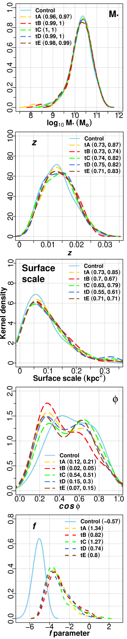
Figure 1: Fundamental properties: Kernel density estimations for the distributions of fundamental M_∗ and z (top). Distributions of surface scale, inclination angle ($\phi$) and f parameter are also included (middle to bottom). The perturbed samples, trials A to J, are shorten as tA to tJ. For M_∗ to $cos\,\phi$, results from the Anderson-Darling (AD) and permutation (equal densities) tests are shown for each perturbed sample against the control one. The skewness ($S$) as a normality test, is shown for the f parameter. Decisions are fairly normal ($-0.5\leq\,S$ $\leq 0.5$), moderately skewed ($-1\leq\,S<\,-0.5$, $0.5\,<S\,\leq 1$) and highly skewed ($S<\,-1$, $S>\,1$).

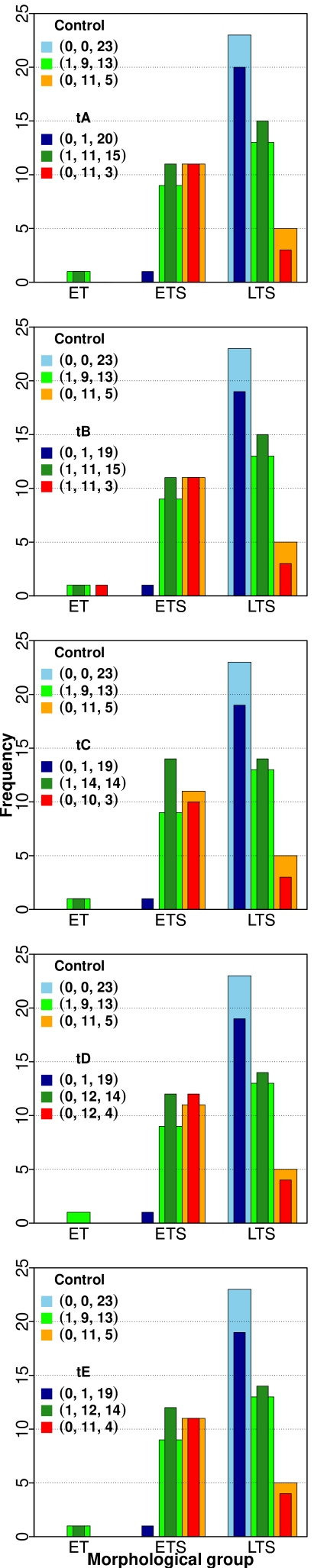
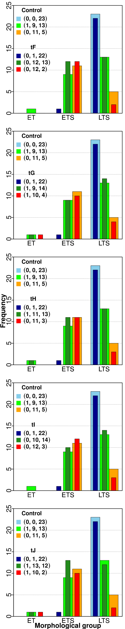
Figure 2: Fundamental properties: the morphological group-galaxy colour relation between control (Control) and perturbed samples (tA to tJ). Colour frequencies in parenthesis are ordered by morphological group (i.e. early type, ET; early type spiral, ETS; late type spiral, LTS).

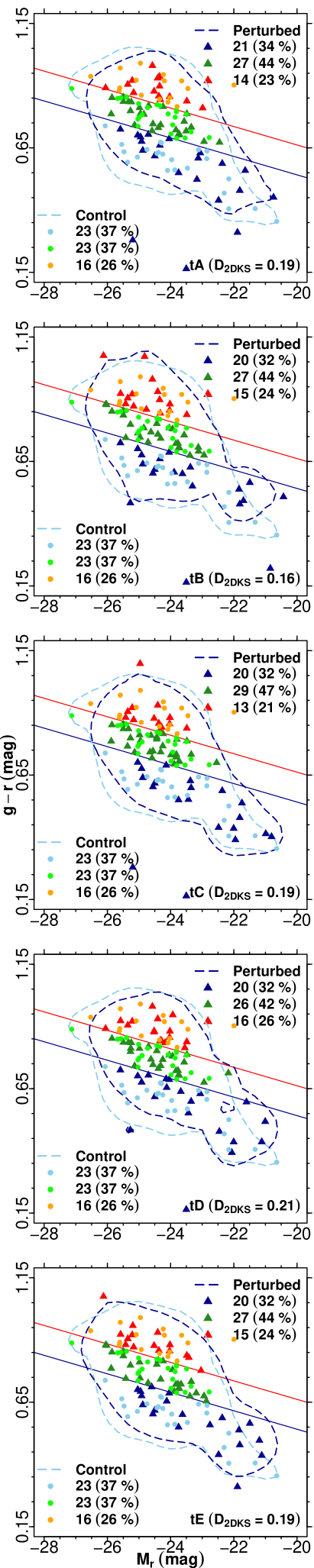
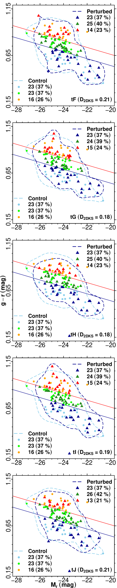
Figure 3: Fundamental properties: CMDs showing the distributions for control (Control) and perturbed samples (tA to tJ). The colour solid lines are explained in Section 2.2. The number of colour galaxies with their respective percentages, as well as 0.1 Kernel density contours (dashed lines) are indicated for each sample. From the 2D K-S/Peacock two-sample test, each bottom-right corner gives the maximum absolute difference (D_2DKS) between each empirical cumulative probability distribution.

3.4 Sample comparison

Contrasts in spatial scales of the single star-forming regions and in galaxy inclinations with respect to the plane of the sky can be both sources of observational bias. Density estimations for the spatial or surface scale, cos $\phi$ and f parameter distributions are shown in Fig. 1 (see also Table LABEL:tab:A1). For surface scales, the dashed-line distributions resemble the control one with statistical results of at least 0.6. These scales directly depend on z so the density estimations and statistical results of the scales will always be as good as those of z. In contrast, the cos $\phi$ distributions are the odd case. The density estimations evidently differ: the perturbed samples are biased towards larger inclinations. We therefore relocate the coordinates of each spaxel by deprojecting them on those galaxies that show a disk component. The number of non-deprojected cases is larger for the perturbed samples (tA to tJ) consequence of their higher bias. Non-deprojected cases, i.e. low cos $\phi$ values for trials tA to tJ are 13, 17, 8, 11, 15, 12, 16, 13, 13, and 17 respectively. Likewise, they are 6 for the control sample. Regarding the f parameter distributions, skewness is used as a measure of normality. The control sample distribution, close to be fairly normal, is moderately (negatively) skewed. On the contrary, the distributions of the perturbed samples are positively skewed, most of them highly (outliers).

Having shown alike surface scales for resolved regions, we now explore contrasts in frequencies of star-forming regions among samples and per single galaxy. Table 2 lists these frequencies by splitting the control and perturbed samples according to the source of gas excitation. No known phenomenon prevents most of the available gas to turn into stars in SFG Blue and SFG LTS objects so both are the ones shown apart only for the sake of briefness. SFG Green and SFG Red types are included in the SFG subsample and are shown apart from Section 4 on. Even fairer comparisons will be conducted adopting this subsampling (not done in AGN-like galaxies due to the size limitation). Notice, from Table 2 (top), well balanced galaxy frequencies. In the case of the totals of star-forming regions (Table 2, middle), disproportions are the lack of SFG Blue early type spirals (ETSs) in control galaxies and the AGN-like case of perturbed galaxies almost doubling those frequencies of control ones (by a factor of $\sim$1.9). This last contrast is not expected since differences in galaxy frequencies are not as great as double. Even the respective z distributions exhibit no marked biases. Moreover, excluding the AGN-like subsample (with factors of $\sim$1.3 and $\sim$1.6), median and mean frequencies per single galaxy (Table 2, bottom) differ not much (largest factors are of $\sim$1.1). Anderson-Darling (AD) tests for the distributions of numbers of star-forming regions support this. Likelihoods are 0.59, 0.58, 0.75 and 0.48 for SFG Blue, SFG LTS, SFG and AGN-like respectively. In sum, numbers of star-forming regions in AGN-like galaxies are the most dissimilar ones.

Table 2: Frequency summaries of galaxies (top) and star-forming regions (middle) as defined in Section 2.3.1. Star-forming region statistics per single galaxy (bottom).

	Control					Perturbed
	SFG	SFG		AGN		SFG	SFG		AGN
	Blue	LTS	SFG	-like		Blue	LTS	SFG	-like
ETSs	$\ldots$	$\ldots$	12	09		01	$\ldots$	13	11
LTSs	23	40	40	01		20	37	37	1
Total	23	40	52	10		21	37	50	12
ETSs	$\ldots$	$\ldots$	04 396	1 024		01 462	$\ldots$	05 818	1 900
LTSs	21 223	31 001	31 001	0 218		20 803	31 907	31 907	0 412
Total	21 223	31 001	35 397	1 242		22 265	31 907	37 725	2 312
median	925	746	628	098		0 894	713	628	127
mean	923	775	681	124		1 060	862	754	193
$\sigma$	442	428	435	093		0 664	599	586	157

3.5 H$\alpha$ flux percentage radii

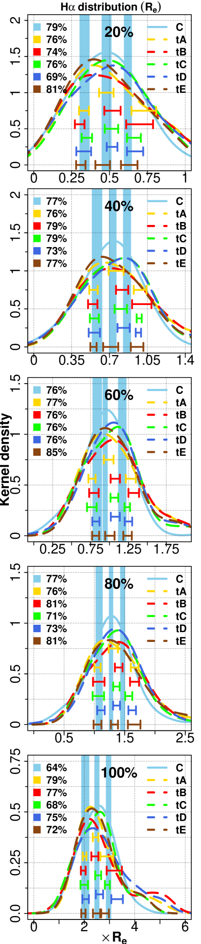
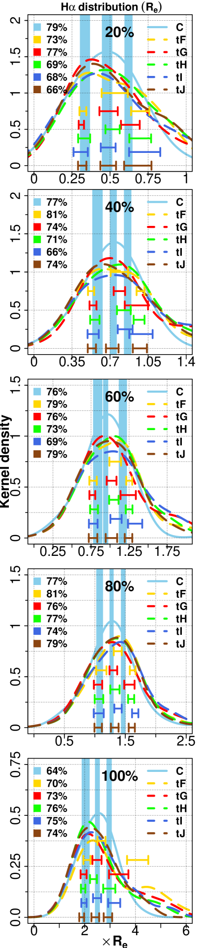
Figure 4: Kernel density estimations for our H$\alpha$-flux-percentage radius/R_e fractions, i.e., the H$\alpha$ emission line distribution as a function of R_e (20 to 100 %, from top bottom). Control (C) and perturbed samples, trials A to E and F to J (tA to tE, left and tF to tJ, right). At each left are the percentages of fractions (one fraction per galaxy) within $\pm$ 1 $\sigma$ width centred at each distribution median. Light-blue columns are the Monte Carlo standard deviations (MCsds, i.e. $\pm$ 1 $\sigma$ width from Monte Carlo simulations) corresponding to and centred at the 1st, 2nd (median) and 3rd quartiles (Qs) of the control distribution. Likewise, coloured ranges represent the same for each perturbed sample distribution.

All annular profiles compile single-galaxy data and depict each sample or subsample SP properties by concentric annuli. These are defined by the boundaries of deprojected radii which encircle percentages of the all-excitation H$\alpha$ flux (20, 40, 60, 80 and 100 %). From each galaxy set of spectra solved by starlight, the total H$\alpha$ flux is computed by ignoring the excitation source and flux outliers. The flux percentages are then computed and so the encircling radii. Since such those fluxes are meant for sectioning only, they are not extinction-corrected. Besides, their respective spectra sometimes show no H$\beta$ line emission detections (poor line S/N ratios). See Appendix B for an additional but important note on these annular profiles.

As noticed already, the H$\alpha$ flux, related to the data per se, is used to depict the radial extension instead of photometric extents such as the effective radius (R_e). To prove the reliability of the encircling-H$\alpha$-flux radii, Fig. 4 plots Kernel density estimations of the H$\alpha$ emission line distribution of our sampled galaxies as a function of R_e (half-light radius of the r band in an elliptical aperture, see W-14). Table 3 lists medians, 3rd quartiles (Qs) and standard deviations. Statistical test results between samples for the sets of these radial fractions are also included. At each percentage radius/R_e fraction in Fig. 4 (panels 20 to 100 %), numbers at left indicate the percentages of fractions (one fraction per galaxy) close to the median of each respective set, i.e., within $\pm$ 1 $\sigma$ width range centred in the median. In general, a bit more than a 70 % of the fractions are near the median in each distribution. Moreover, medians of fractions in Table 3 are in good agreement with the standard definition of R_e. For instance, medians for the mid-radius (60 %) are the ones closest to unity (see also Table LABEL:tab:A1). These H$\alpha$ flux percentage radii are then credible distance normalizers and may be used as indicators of galaxy extensions.

From Monte Carlo simulations, standard deviations (MCsds) for medians, 1st and 3rd Qs are obtained for the distributions of percentage radius/R_e fractions. They are drawn as columns for the control sample, and as ranges for trials tA to tJ (see Fig. 4). If contrasting the ranges with respect to the columns, the former are biased towards higher fractions, specifically, medians and 3rd Qs. Also see that the curves are much different from the 1st Q on (right skewed). If comparing medians and 3rd Qs by computing fractions from Table 3, we find no significant difference for medians: 31/50 fractions advantage perturbed samples by $<$10 %. Third Qs are slightly different: 27/50 fractions advantage perturbed samples by $>$10 %. Differences in standard deviations are the most significant: 33/50 advantage perturbed galaxies by $>$20 %. We look at last at the statistical tests (AD-P) of Table 3. If arranging the likelihoods in the $l>$0.5, 0.25$<l\leq$0.5 and $l\leq$0.25 groups, frequencies for AD-permutation tests are respectively 6-4, 15-17 and 29-29. A likelihood for similitude of $\leq$0.25 describes the most both sample distribution functions. In sum, it may be said that the H$\alpha$ line emission appears to be a little more dispersed for perturbed galaxies.

4 Results

Table 3: Medians, 3rd quartiles (Qs) and standard deviations (median-3rdQ-$\sigma$) of the percentage radius/R_e fractions (e.g. $\times$ R_e). AD and permutation test results (AD-P) for each radial set of fractions between control and each perturbed sample (tA to tJ) are also listed.

H$\alpha$ flux percentage radii
20%	40%	60%	80%	100%
Control
0.48-0.62-0.27	0.73-0.86-0.30	0.94-1.17-0.33	1.28-1.47-0.40	2.50-2.96-0.63
tA
0.48-0.73-0.33	0.76-0.98-0.38	0.99-1.28-0.40	1.31-1.67-0.48	2.45-2.89-0.89
0.27-0.26	0.22-0.18	0.20-0.24	0.16-0.12	0.41-0.18
tB
0.52-0.70-0.34	0.82-1.00-0.44	1.08-1.32-0.49	1.40-1.66-0.60	2.42-3.19-1.09
0.24-0.23	0.11-0.11	0.06-0.10	0.06-0.09	0.21-0.06
tC
0.51-0.66-0.29	0.80-0.97-0.36	1.06-1.23-0.38	1.36-1.57-0.43	2.55-2.91-0.77
0.54-0.80	0.21-0.36	0.17-0.28	0.23-0.37	0.81-0.76
tD
0.52-0.67-0.27	0.83-0.97-0.33	1.08-1.25-0.35	1.37-1.62-0.38	2.60-3.30-0.98
0.46-0.49	0.24-0.28	0.24-0.44	0.26-0.34	0.18-0.16
tE
0.45-0.63-0.31	0.71-0.95-0.38	1.00-1.24-0.42	1.33-1.66-0.56	2.49-2.82-0.75
0.81-0.61	0.36-0.28	0.19-0.51	0.12-0.23	0.75-0.39
tF
0.53-0.70-0.31	0.79-0.98-0.42	1.07-1.25-0.47	1.38-1.62-0.62	2.66-4.09-1.31
0.28-0.25	0.17-0.21	0.12-0.19	0.09-0.30	0.02-0.01
tG
0.49-0.63-0.29	0.79-0.94-0.37	1.02-1.24-0.45	1.30-1.57-0.52	2.49-3.34-1.14
0.51-0.36	0.21-0.16	0.22-0.24	0.44-0.38	0.10-0.01
tH
0.52-0.70-0.28	0.83-0.97-0.34	1.05-1.25-0.37	1.33-1.60-0.46	2.35-2.97-0.96
0.32-0.30	0.22-0.21	0.20-0.24	0.34-0.39	0.27-0.04
tI
0.49-0.73-0.34	0.84-0.98-0.41	1.08-1.33-0.46	1.38-1.66-0.51	2.49-3.16-1.00
0.23-0.11	0.08-0.02	0.05-0.03	0.08-0.13	0.29-0.15
tJ
0.49-0.68-0.27	0.72-0.97-0.36	1.02-1.24-0.42	1.33-1.61-0.47	2.42-2.92-0.82
0.43-0.24	0.29-0.11	0.28-0.32	0.33-0.46	0.54-0.25

4.1 Resolved SFMSs

Table 4: Frequency summary from the annular comparisons between samples for all subsamples (see Table LABEL:tab:C1). Numbers in parenthesis are totals of star-forming regions and annular means. Columns titled as “Fig. 5” list the frequencies from the comparisons in Fig. 5. Acronyms (first column) mean frequencies of Different Slopes (DS), of Perturbed samples having the Flattest slope (PF) and frequencies of Different Distribution functions (DD).

Annuli (H$\alpha$ flux percentages)

Fig.

Annuli (H$\alpha$ flux percentages)

Fig.

20%

40%

60%

80%

100%

5

20%

40%

60%

80%

100%

5

AGN-like (36 552, 7 310)

SFG Red (68 654, 13 731)

DS

10/10

07/10

03/10

07/10

10/10

4/5

08/10

06/10

04/10

07/10

10/10

4/5

PF

00/10

00/7

03/3

01/7

10/10

1/4

03/8

04/6

00/4

00/7

03/10

1/4

DD

07/10

9/10

09/10

9/10

010/10

5/5

10/10

9/10

09/10

08/10

010/10

5/5

SFG ETS (122 322, 24 464)

SFG Green (208 180, 41 636)

DS

08/10

10/10

9/10

08/10

010/10

5/5

08/10

06/10

03/10

04/10

08/10

4/5

PF

01/8

00/10

00/9

00/8

00/10

0/5

00/8

02/6

03/3

04/4

08/8

3/4

DD

10/10

10/10

09/10

10/10

010/10

5/5

10/10

09/10

09/10

10/10

08/10

5/5

SFG Blue (376 698, 75 340)

SFG LTS (531 210, 106 242)

DS

09/10

10/10

10/10

02/10

03/10

3/5

10/10

10/10

10/10

06/10

05/10

5/5

PF

09/9

10/10

10/10

01/2

02/3

3/3

10/10

10/10

10/10

06/6

04/5

5/5

DD

9/10

10/10

10/10

09/10

09/10

5/5

10/10

10/10

10/10

06/10

10/10

5/5

SFG (653 532, 130 706)

All (690 084, 138 017)

DS

09/10

10/10

010/10

05/10

05/10

5/5

09/10

10/10

10/10

07/10

08/10

5/5

PF

09/9

10/10

010/10

05/5

04/5

5/5

09/9

10/10

10/10

07/7

08/8

5/5

DD

10/10

10/10

10/10

08/10

10/10

5/5

10/10

10/10

10/10

09/10

10/10

5/5

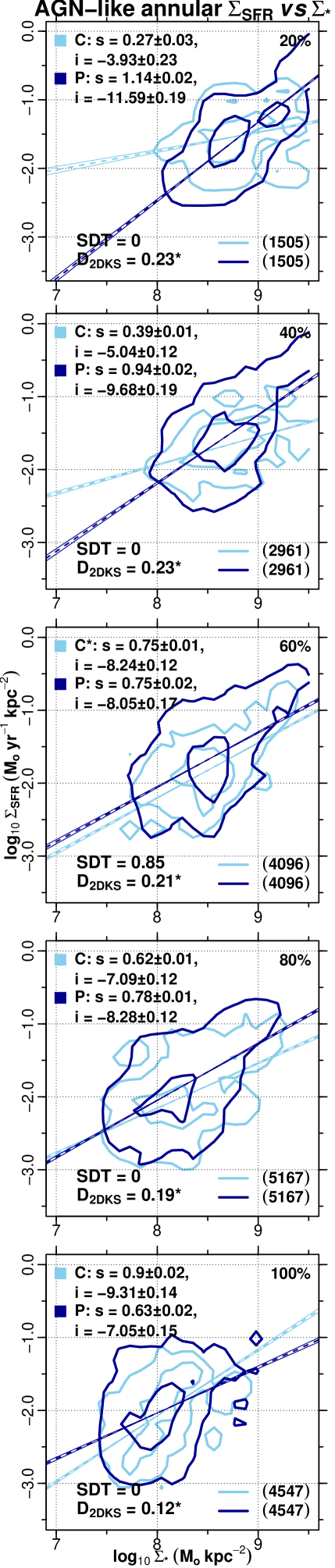
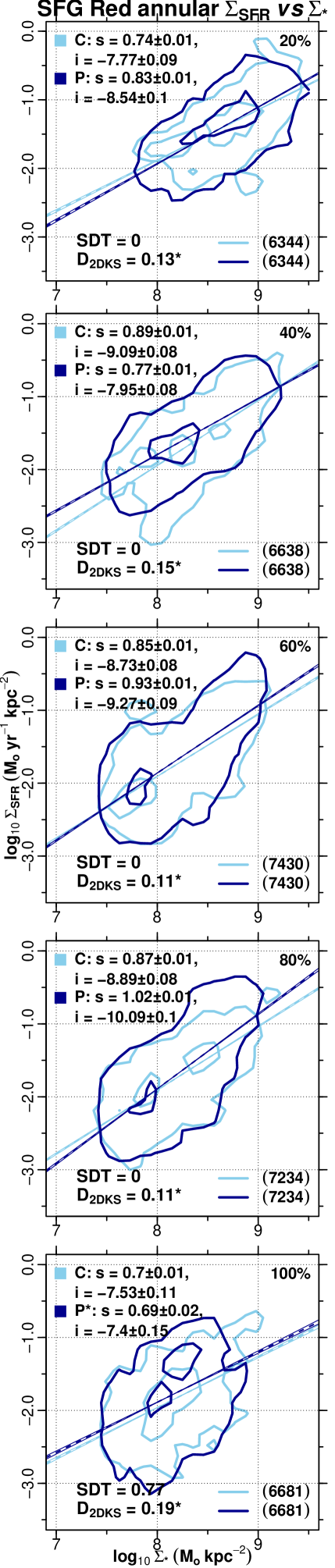
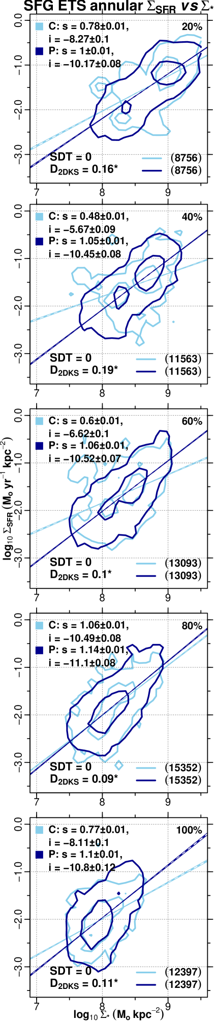
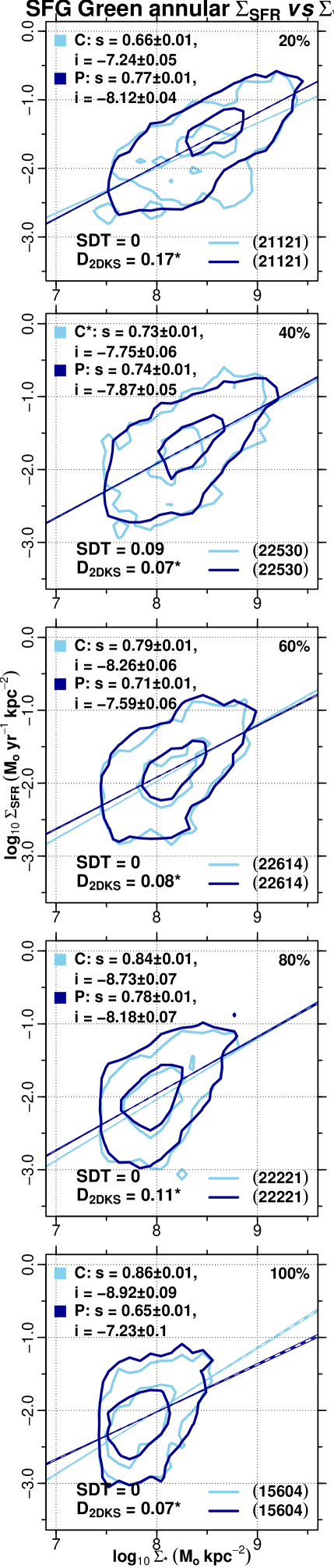
Figure 5: Annular-resolved SFMSs. The perturbed star-forming regions (dark blue) are paired with their control ones (light blue) closest in $\mathrm{\Sigma}_{*}$ (i.e., paired by the minimum $\mathrm{\Sigma}_{*}$ difference). All star-forming regions in each comparison set (i.e. trials tA to tJ each one with its respective control sample regions, see Appendix C) are considered in order to get average linear model coefficients. From left to right: Kernel density estimations (0.1 and 0.9 contour densities from outside-in) of the star-forming regions inhabiting AGN-like, SFG Red, SFG ETS and SFG Green galaxies. Control (C) and perturbed (P) linear regression coefficients: slope (s) and intercept (i) (models for all annular sequences are statistically significant). Though not perceptible in all annuli, the error intervals are drawn for all fits. Asterisks indicate, from significance difference tests (SDTs), the sample (C or P) with s closer to that one if combining both-sample regions (Section 5.4). Likewise, SDTs are shown for each pair of sample slopes. 2D K-S/Peacock two-sample test differences ($\mathrm{D_{2DKS}}$, Yuanhui, 2017) are finally included. Asterisks indicate that both distribution functions come from a different parent distribution.

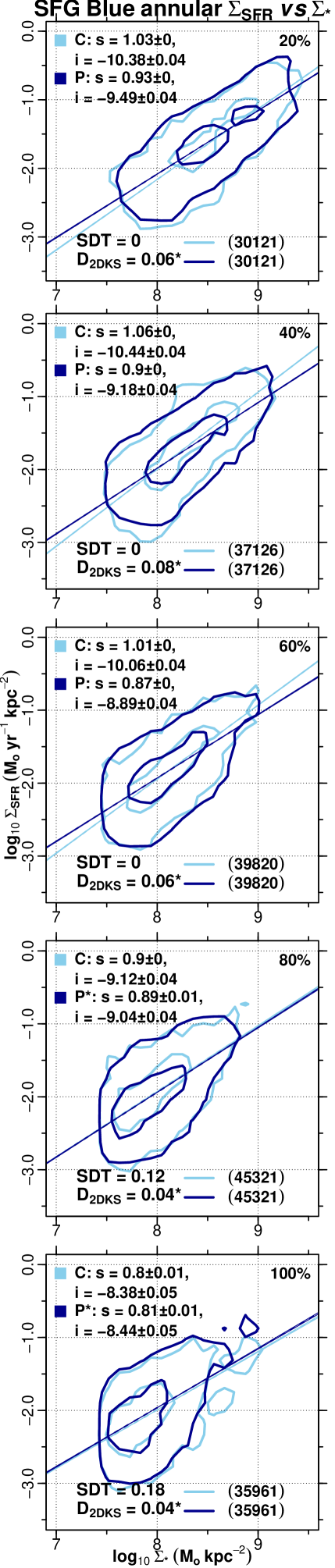
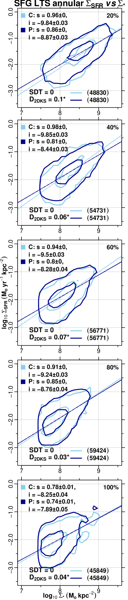
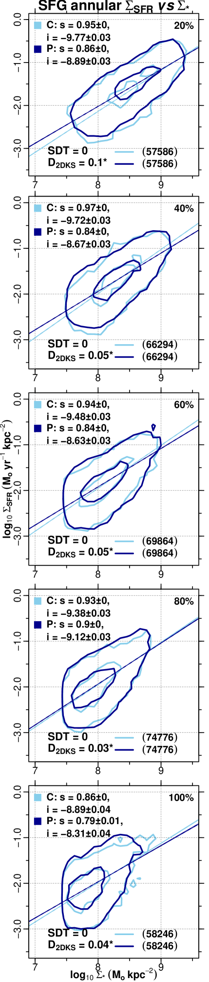
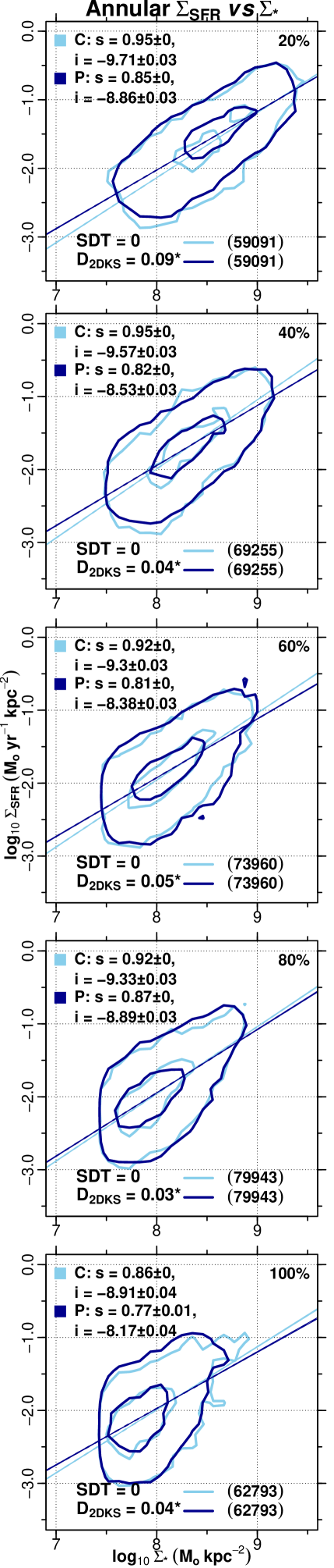
Figure 5: Annular-resolved SFMSs (cont.). Same caption as above but for SFG Blue, SFG LTS, SFG and all galaxies.

Galaxies with H ii regions, small fractions of old stars and little light concentration yield the SFMS, the tight correlation of both global M_∗ and SFR. It has been confirmed that a local (resolved) correlation also holds for $\Sigma_{*}$ and $\mathrm{\Sigma_{SFR}}$ (e.g. Sánchez et al., 2013; Cano-Díaz et al., 2016; González-Delgado et al., 2016; Hsieh et al., 2017; Cano-Díaz et al., 2019; Vulcani et al., 2019). Analyses which evidence the global correlation as a consequence of the resolved one have increased recently. However, Erroz-Ferrer et al. (2019) and Cano-Díaz et al. (2019) (hereafter CD-19) have shown that regions with low $\Sigma_{*}$ noticeably flatten the resolved relation. CD-19 exhibit that below the 7.5 M_⊙ kpc^-2 threshold, H$\alpha$ flux detection limits, apertures and other observational constraints affect the data and they warn about them in other surveys. Similarly, Hall et al. (2018) find that galaxies and regions of others spatially below this threshold do not follow the SFMS. Due to this issue, from this Section on and in Appendices B and C, we treat only star-forming regions above the CD-19 threshold.

Table LABEL:tab:C1 lists, in annular comparison sets, the linear regression coefficients of control and perturbed samples (tA to tJ) on the SFMS plane. Specifically, slopes for the same predictor ($\Sigma_{*}$) across two models (control and perturbed galaxies) are compared. To do so, an interaction term between samples and $\Sigma_{*}$ is included in the model function. In this way, the p-value of the interaction term represents a significance difference test (SDT) between both sample slopes. Importantly, sample slopes are suggested to be different when the SDT value falls below the statistical level. In each comparison set of Table LABEL:tab:C1, slopes marked with * are the closest ones to the slopes resulting from combining both sample data (a topic treated afterwards, Section 5.4). Only SDTs with values above the statistical level are considered for this and that slope with the highest test value is marked. On the other hand, for comparisons, only cases of different slopes are used. Lastly, from the K-S/Peacock two-sample test, $\mathrm{D_{2DKS}}$ differences marked with * reject the null hypothesis of a parent distribution as the origin. With all this in mind, we summarize Table LABEL:tab:C1 comparisons between samples for all subsamples in Table 4.

Starting with frequencies of Different Slopes (DS), annuli having those greater than 5/10 are identified. Notice that at least in 3/5 annuli this condition is satisfied. That is the case of SFG Green, SFG Blue and SFGs. SFG ETS and all galaxies meet the condition in all annuli. So, in general, models of linear regression (slopes) on the resolved SFMS differ between control and perturbed samples. Second, from the above cases of different slopes, we find those in which the Perturbed sample has the Flattest slope (PF). Similarly, we distinguish those annuli in which the fraction exceeds a half. This restriction is poorly met in AGN-like and SFG Red objects (2/5, 1/5 annuli respectively) and is not in SFG ETSs. For the others occurs the opposite: 3/5 annuli for SFG Green, 4/5 for SFG Blue and 5/5 for the rest. This means, for both samples, that the $\Sigma_{*}$-$\Sigma_{\mathrm{SFR}}$ relation might be correlated with the galaxy subsample (the stellar mass concentration specifically). Finally for all annuli, and regardless of the subsample, the 2D distributions of control and perturbed samples point to differ in regard of their origins. All fractions of frequencies of Different Distribution functions (DD) are greater than a half.

To explore the mean trends of linear regression models of all samples on the SFMS plane, Fig. 5 plots all star-forming regions in the annular comparison sets of Table LABEL:tab:C1. In the same way, columns of Table 4 allusive to Fig. 5 list the annular frequencies result of the sample comparisons. DS frequencies are found in at least 3/5 annuli so, on average, linear regression slopes differ too. The previous trend of PF frequencies repeats: the lowest fractions belong to AGN-like, SFG Red and SFG ETS objects whereas a significant increment starts from the SFG Green subsample. As same as before, regardless of annulus and subsample, the 2D distributions do not share a parent one as a common origin.

Moreover, some important notes from inspecting Fig. 5.

• By concentric annuli:

  1. All positions of 0.1 and 0.9 contour densities clearly show a trend of both $\Sigma_{*}$ and $\Sigma_{\mathrm{SFR}}$ decreasing from the centre (Maragkoudakis et al., 2017).

  2. The standard deviations of both s and i diminish from the centre for control but remain rather constant for perturbed galaxies. Picturing the stellar dynamics might distinguish perturbed galaxies as having disordered SF processes along all annuli.

  3. Excluding SFG Red objects, the highest $\mathrm{D_{2DKS}}$ differences go inwards. This might support contrasts in the transfer of gas to the centres.

• By galaxy subsamples:

  1. Compared with those of all galaxies, the density distributions of AGN-like, SFG Red, SFG ETS and SFG Green objects are quite unlike. The most dissimilar distributions between samples belong also to these galaxies (greater $\mathrm{D_{2DKS}}$ differences). Section 5 explores whether these facts are consequence of the amounts of star-forming regions that inhabit each subsample (see Table 4).

  2. As noticed already, a singular trend characterizes the flattening/steepening of the sample slopes. That trend might depend on the stellar mass concentration that according to the literature may distinguish our subsamples (AGN-like, SFG Red and SFG ETS objects distinguished by the highest $\Sigma_{*}$ values, e.g. Appendix B). By finding steeper slopes for Sc-Scd/Sd-Sdm types in the disk-component SFMS, Catalán-Torrecilla et al. (2017) propose quenched SF in Sb-Sbc more massive disks. Following this, control AGN-like, SFG Red and SFG ETS galaxies would be at a quenching stage. The same for perturbed SFG Green, SFG Blue, SFG LTS, and SFG galaxies. Section 5 explores whether suppressions or (re)activations of SF (quenching or rejuvenation) are at play.

In sum, on the SFMS plane, star-forming regions in control and perturbed galaxies show models of linear regression that differ, inclinations of the model fits that depend on the galaxy subsample and 2D distributions with unlike origins.

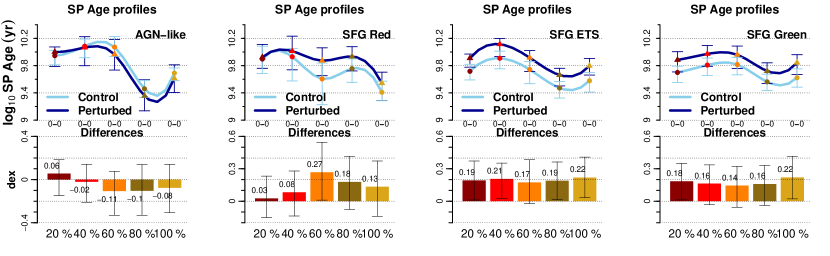
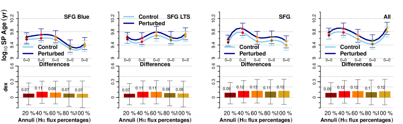
Figure 6: Annular profiles: SP age. All profiles use the amounts of annular star-forming regions per sample and subsample as in Fig. 5. Five consecutive-outward annuli denote the radial extension (see Section 3.5). “Differences” (bar heights by always subtracting the control values from the perturbed ones) are the medians of the annular distributions of differences (differences by pairing sample spaxels which are the closest in $\mathrm{\Sigma_{*}}$). Bar lines depict the interquartile ranges (IQRs, 1st to 3rd) of the distributions of differences. Symbols are both sample values giving each Difference. Symbol lines depict the IQRs of the annular distributions. On each pair of these, AD-permutation tests are performed (likelihoods right below the profiles).

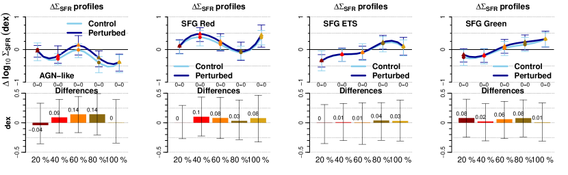
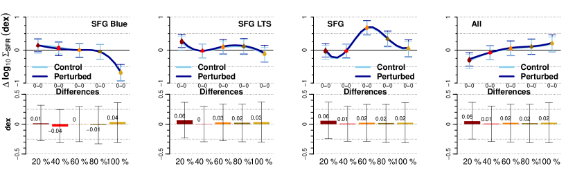
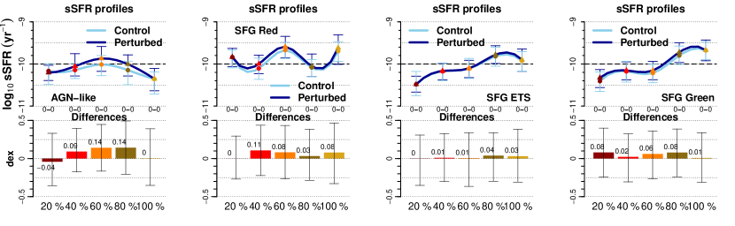
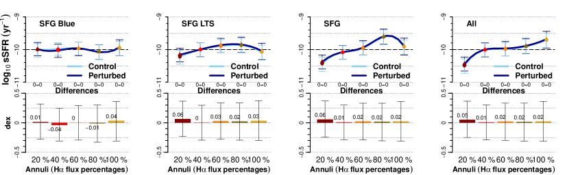
Figure 7: Annular profiles: (top) $\mathrm{\Delta\,\Sigma_{SFR}}$ using the annular linear fits of all sampled regions on the SFMS plane, (bottom) sSFR ($\mathrm{\Sigma_{SFR}}\,\Sigma_{*}^{-1}$) where dashed lines denote the Peng et al. (2010) threshold between SFGs and quiescent objects. Same information as in caption of Fig. 6.

4.2 Annular profiles

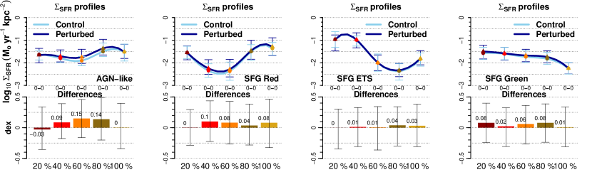
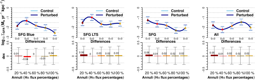
Figure 8: Annular profiles: $\mathrm{\Sigma_{SFR}}$. Same information as in caption of Fig. 6.

The distributions of the profiled SP properties along this work belong to all regions in the annular sets of comparisons of Table LABEL:tab:C1. So, as in Fig. 5, our profiles show the median trends across trials tA to tJ all against the control sample. Figures 6 and 7 profile the SP age, $\mathrm{\Delta\,\Sigma_{SFR}}$ and sSFR. “Differences” are the medians of the annular distributions of differences whilst symbols are both sample values giving those Differences. Line segments are the corresponding interquartile ranges (IQRs) of each respective distribution. Between samples, the distributions are compared by AD-permutation tests (likelihoods right below the profiles). Starting with age and excluding the AGN-like subsample, star-forming SPs are clearly older for perturbed samples. Differences and their IQRs are significantly extended above zero dex whereas most of the corresponding ones for AGN-like objects are well below. IQRs of symbols for AGN-like objects between samples clearly differ too. In perturbed galaxies of this type, SPs but the central ones tend to be younger.

Figure 7 (top) profiles the offsets with the annular SFMSs of the SPs in all galaxies regardless of the samples. Notice clear Differences, favorable for perturbed samples, in AGN-like, SFG Red and SFG Green objects. Major extensions of the IQRs are above zero in 3/5 annuli and IQRs of symbols in those annuli are the most dissimilar. Perturbed SFG LTS, SFG and all type galaxies show favorable slight Differences only in the centres. Major extensions of IQRs of these Differences are clearly above zero. Total extensions of IQRs for central symbols of these perturbed subsamples are slightly biased towards higher offsets. For SFG ETS and SFG Blue subsamples, there are no consequential Differences ($<$10 %). IQRs of their Differences are more balanced around zero. Moreover, only the control AGN-like subsample has negative offsets (reduced) along all annuli. Reduced cases are also those of SFG ETS, SFG Green and all types: no matter the samples, IQRs of central symbols are totally below zero and increments towards the periphery are apparent.

Notice the Differences and their IQRs of the sSFR (Fig. 7 bottom) in good agreement with those of the $\mathrm{\Delta\,\Sigma_{SFR}}$. On this basis, all notes regarding the $\mathrm{\Delta\,\Sigma_{SFR}}$ are valid for the sSFR. Moreover, the threshold of Peng et al. (2010) serves as a similar reference as the zero line for the $\mathrm{\Delta\,\Sigma_{SFR}}$. Based on this, two similarities and two discrepancies can be seen between the $\mathrm{\Delta\,\Sigma_{SFR}}$ and sSFR profiles. These are respectively: 1) SFG ETS, SFG Green and all types keep showing clear increments from the centre (SFG LTS and SFG sSFR profiles now added); 2) unexpectedly, SFG Red objects centrally increased in $\mathrm{\Delta\,\Sigma_{SFR}}$ and above the threshold in sSFR; 3) centres of galaxies in all subsamples but SFG Red and SFG Blue being below Peng et al. 2010 threshold (including their IQRs) and; 4) SFG Blue objects having a flat sSFR profile along the threshold. On the other hand, recall the younger SPs in perturbed AGN-like galaxies. Two facts now certainly explain this singularity: 1) regions in this subsample are increased in $\Sigma_{\mathrm{{SFR}}}$ and are currently more able to form stars (e.g. Sánchez et al., 2018b) and 2) perturbed AGN-like galaxies contain almost twice as many star-forming regions than their control analogues (Table 2).

The $\mathrm{\Sigma_{SFR}}$ is next profiled in Fig. 8. The agreement of the Differences and their IQRs between $\mathrm{\Delta\,\Sigma_{SFR}}$ and sSFR apparently persists in the $\mathrm{\Sigma_{SFR}}$. This is a mere coincidence and has nothing to do with a common property ($\mathrm{\Sigma_{SFR}}$) influencing the computations. The previous allows us to state, as in the case of $\mathrm{\Delta\,\Sigma_{SFR}}$ and sSFR, that the favorable Differences for perturbed samples are: 1) mostly dominant in AGN-like, SFG Red and SFG Green subsamples (3/5 annuli); 2) little, but evidently increased only centrally in SFG LTS, SFG and all subsamples and; 3) very likely, neither increased nor reduced in SFG ETS and SFG Blue ones. Notice, in addition, that the statistical tests on the annular distributions result in the lowest likelihoods regardless of the property and subsample.

In general, the SFR properties of regions in perturbed galaxies are practically never inferior. This is despite the fact that these regions are older.

5 Discussion

5.1 Amounts of regions and their SFMS distributions

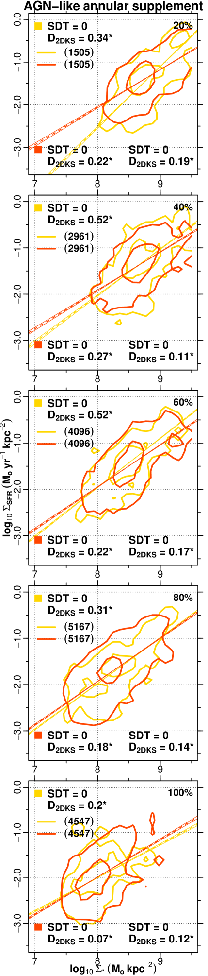
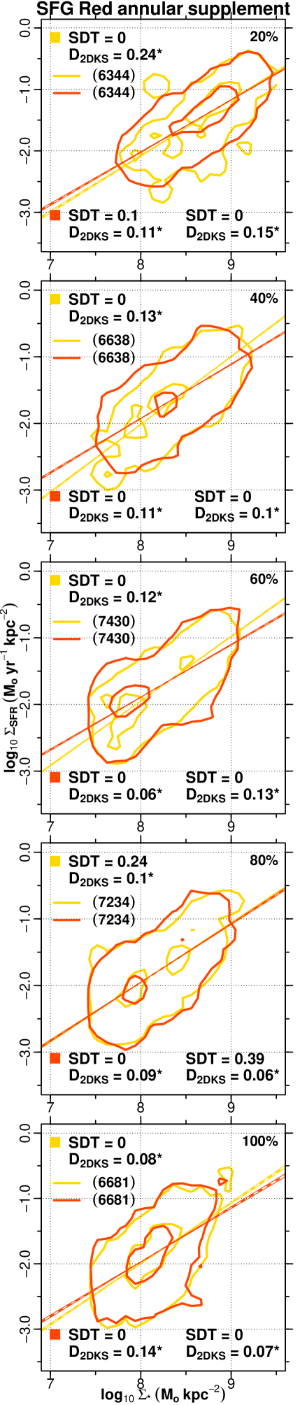
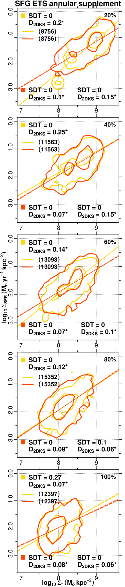
Figure 9: Supplemental, annular-resolved SFMSs. Perturbed star-forming regions (red) are paired with their control ones (gold) at the closest $\mathrm{\Sigma}_{*}$. All supplemental star-forming regions in each comparison set (i.e. trials tA to tJ each one with its respective control sample regions, see Appendix C) are considered. From left to right: Kernel density estimations (0.1 and 0.9 contour densities from outside-in) of the supplemental star-forming regions corresponding to AGN-like, SFG Red, SFG ETS and SFG Green galaxies. Models for all annular sequences are statistically significant (error intervals are drawn for all fits). SDTs and $\mathrm{D_{2DKS}}$ differences (asterisks indicate both distribution functions coming from a different parent one) following colour squares (gold, control; red, perturbed) give the test results between regions (Fig. 5 1st part) and their supplemental ones within the same sample. SDTs and $\mathrm{D_{2DKS}}$ differences at the bottom-right give the results between supplemental regions only.

In Section 4.1 we show that the density distributions on the SFMS plane of four subsamples: AGN-like, SFG Red, SFG ETS and SFG Green, are dissimilar compared with those of all subsamples. Between samples, $\mathrm{D_{2DKS}}$ differences are also greater among these subsamples than those among the other types. Table 4 lists the totals of star-forming regions used in each subsample. Notice a significant unbalance for AGN-like, SFG Red, SFG ETS and SFG Green subsamples with respect to the rest. To get a better understanding of a possible dependence of the SFMS distributions (the density distributions on the SFMS plane) on the amount of star-forming regions, in Fig. 9 we show the supplemental SFMSs. These help to characterize regions from all galaxies except those corresponding to each one of the four subsamples, i.e., Fig. 5 1st part. Notice that the selection of these supplemental regions is done at the closest $\Sigma_{*}$ values. These supplemental regions are distinguished either within control (gold contours) or within all the perturbed samples (red contours). The reasoning is the following: if the parameters derived from these supplemental distributions are alike to those of Fig. 5 1st part, we would prove a dependence on the amount of regions. The contrary would mean that the SF processes (which characterize the regions and the supplemental ones) are different.

It turns out from Fig. 9, that SDTs point to equal slopes in only four annuli: two for SFG Red (20 and 80 % annuli, red and gold squares) and one for SFG ETS and SFG Green each (100 and 100 % annuli, gold and red squares, respectively). Regarding $\mathrm{D_{2DKS}}$ differences, all suggest that the density functions being compared do not have their respective origins in a common parent distribution. In sum, there are no similitudes between regions and their supplemental ones, at the closest $\Sigma_{*}$ values and at the same number of regions for the perturbed samples and the control one. The dissimilarities between density distributions mentioned above do not depend neither on the amounts nor on the stellar mass concentration of the regions. On the other hand, by looking at the parameters comparing both supplemental regions between samples (bottom-right in all panels of Fig. 9), in 18/20 annuli, the SDTs suggest different slopes. From these frequencies, the fit corresponding to perturbed samples (red) is the flattest in 16 cases ($\mathrm{D_{2DKS}}$ differences also point to uncommon origins). Therefore the linear fits, either flatter or steeper, do not depend on the $\Sigma_{*}$ of the regions but on some other property characterizing the galaxy types defining our subsamples. A possible explanation involving the M_∗ along with the perturbation parameter is treated in Section 5.3.

The one certainty is that most of the slopes for perturbed objects are flatter, than the corresponding ones for control objects, at the $\Sigma_{*}$ values closest to those ones found in AGN-like, SFG Red, SFG ETS and SFG Green types. Concluding, the dominant trend for the galaxies in this study (i.e. the majority of regions, see Table 4) is that perturbed ones show lowered intensities of the SFR with increasing stellar mass density.

5.2 Suppressions and/or (re)activations of SF

Section 4.1 shows slopes with a peculiar behaviour on the SFMS plane. These are flatter and steeper, for control and perturbed galaxies respectively, in AGN-like, SFG Red and SFG ETS objects. Then the slopes switch, to either flatter or steeper, in SFG Green, SFG Blue, SFG LTS, SFG and all objects. Since the former group of subsamples is distinguished by higher concentration of stellar mass (see Appendix B), this peculiar slope behaviour might depend on $\Sigma_{*}$. In the scenario proposed by Catalán-Torrecilla et al. (2017), control AGN-like, SFG Red and SFG ETS galaxies would be at a quenching stage (same for those in perturbed SFG Green, SFG Blue, SFG LTS and SFG subsamples).

However, the results in Section 5.1 suggest that this may not be the case. Steeper slopes for regions in perturbed galaxies do not repeat at stellar mass densities which are the closest to those found in AGN-like, SFG Red, SFG ETS and even SFG Green objects. To clarify on this matter, the SFR ($\mathrm{\Delta\,\Sigma_{SFR}}$, sSFR and $\mathrm{\Sigma_{SFR}}$) profiles (Figs. 7 and 8) are reviewed for traces of suppression (quenching) and/or (re)activation (rejuvenation) of SF. Along each property scale, we contrast the positions of central values relative to those ones of the rest annuli. This approach is justified since changes in central regions (either enhancement or suppression) dominate the regulation of SF (Ellison et al., 2018a).

Starting with the $\mathrm{\Delta\,\Sigma_{SFR}}$, SFG Blue and SFG LTS galaxies show central offsets above the rest annuli. In AGN-like objects, the central offset exceeds three of the rest annuli. SFG Red galaxies have its central offset below three of the rest annuli. The rest galaxy types show evident increments from the centre. Regarding sSFRs, the SFG Red subsample central annulus appears diminished by two annuli. Though quite aligned with all the rest, the central annulus in SFG Blue objects is diminished by two annuli. The central sSFRs and their IQRs in the rest subsamples evidence increments as going outwards (not at all in AGN-like objects due to the periphery). Lastly, the central $\mathrm{\Sigma_{SFR}}$ is diminished against the periphery in AGN-like and SFG Red subsamples. The same may be for all subsamples together. In SFG Blue and SFG LTS types, the central intensity is just diminished against that one of the next annulus. It is in SFG ETS, SFG Green and SFG objects where the centre is evidently dominant. Summarizing, the three profiles show diminished central values (against one annuli at least) in AGN-like, SFG Red and all subsamples. These three types of galaxies are then the clearest ones suffering from quenching.

Though AGN-like types are clear candidates for quenching, some attributes distinguish the perturbed objects. Their age profile indicates younger SPs along all annuli but the central one. In the middle (40, 60 and 80 % annuli), perturbed samples clearly advantage the control one in the three SFR profiles just discussed. In average, numbers of star-forming regions for perturbed samples double control frequencies. This all suggests rejuvenation of the mid-annular SPs in perturbed AGN-like objects.

Finally, the favorable central Differences (Figs. 7 and 8) for perturbed SFG LTS, SFG and, specially, all galaxies, place control objects as the closest candidates for quenching. An interesting fact is why perturbed galaxies mostly exhibit flatter slopes on the SFMS plane (Table 4 and Section 5.1). Perhaps the influence of stellar mass density is somehow weakened. Something else might be regulating the SF in perturbed galaxies.

5.3 A correlation between SF and tidal effects

Peng et al. (2010) estimate the mean local density of galaxies at different redshifts. There are no detectable differences in SFMS and mean sSFR for SFGs between the lowest and highest density Qs. Ellison et al. (2018a) find a similar result. By doing a dynamical analysis, Erfanianfar et al. (2016) compile secure X-ray-detected galaxies to explore the SFMS too. At $0.15<\,z\,<0.50$ they find a flattening caused by red-disk dominated galaxies. Notice that the galactic vicinities in these analyses are expressed by density fields whereas our approach sets the need of ensuring physically related objects, i.e. tidally-related, particularly. As a result, on the SFMS plane, most of the star-forming regions in perturbed galaxies reproduce flatter linear models than those ones for regions in control objects (Section 4.1). This $\mathrm{\Sigma_{SFR}}$ reduction with $\mathrm{\Sigma_{*}}$ points to quenched SF since, indeed, SPs in the perturbed objects are mostly older. However, this assumption is questionable since regions in perturbed objects are practically never inferior in the SFR profiled properties (Section 4.2). Contrasts are clearly favorable for perturbed AGN-like, SFG Red and SFG Green galaxies. For perturbed SFG LTS, SFG and all galaxies, contrasts are also favorable, though only in the centres. Though the SFR profiled properties confirm that a SF suppression has likely started in the centres (Section 5.2), this is regardless of either control or perturbed samples. Moreover, SPs in perturbed AGN-like objects are younger than SPs in their control analogues and the SFR profiled properties of the former are evidently higher. In sum, the flattening on the SFMS plane may not be due to SF quenching but due to a less dependent $\mathrm{\Sigma_{SFR}}$ on $\Sigma_{*}$. Tidal effects might be contributing to drive SF in these regions. This hypothesis would explain the (sometimes little but perceptible) contrasts in the SFR properties.

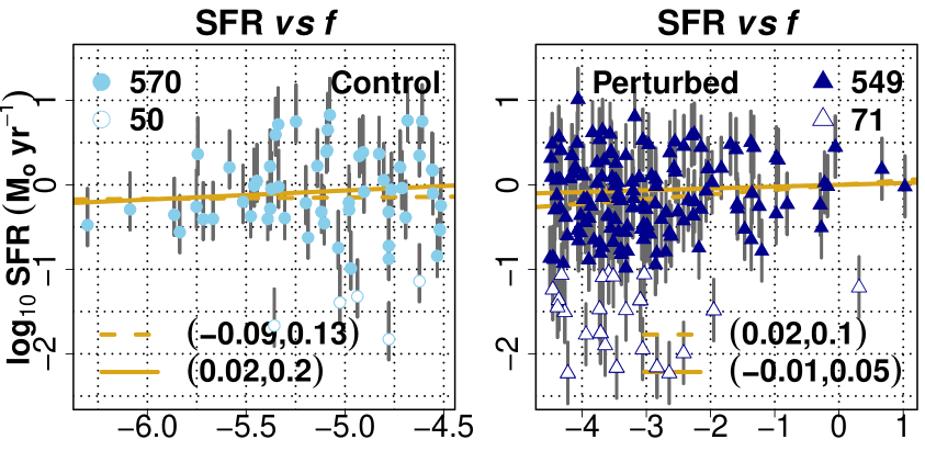
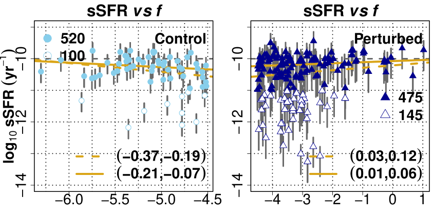
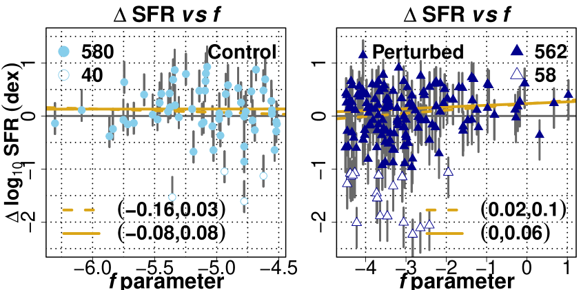
Figure 10: The SFR properties against the f parameter for control (Control) and perturbed (Perturbed, tA to tJ) samples. Black-dashed lines for the sSFR as the Peng et al. (2010) threshold between SFGs and quiescent objects. The SFR offset ($\Delta$ SFR) is computed from a linear fit (SFMS) on the data of all samples. Line segments of points as the IQRs of each property distribution in each sample. Numbers after filled and empty symbols are the frequencies of points above and below, respectively, the thresholds of $-$1, for SFR and $\Delta$ SFR, and $-$11, for sSFR. Gold lines are robust linear model fits, for all points (dashed), and for filled ones (solid). Intervals at 95 % confidence level (bottom) enclose the true values of the model slopes (gold fits). Complementary statistical results in Table 5.

A possible correlation with tidal effects is then explored. We first combined our resolved results alongside the f parameter global measurements (defined in Section 3.1). When pairing the spaxels at a specific value of $\Sigma_{*}$ (the annular median of a galaxy in any sample or the median difference between both annular sets of a galaxy in a sample and the rest galaxies in the other sample) there are always cases of galaxies in a sample with more than one $\Sigma_{*}$ value as the closest to another one of another galaxy in the other sample. This issue makes f parameters to have more than one resolved property value at the same time, having, as a consequence, perceptible effects on the correlation. Notice, in contrast, that our resolved-to-resolved correlations are free from this issue. Figure 10 uses therefore integrated SFR properties of the samples at tight M_∗ distributions (see Fig. 1). As we previously did (Figs. 5 and 9), the average trend is shown for perturbed samples by plotting them altogether alongside versions of the control set. From robust model regression, 95 % confidence intervals of the resultant slopes (gold lines) are included. Moreover, Table 5 lists the summary of the linear model and correlation results. By looking at the gold dashed lines in Fig. 10, notice positive intervals for perturbed samples and negative lower ends for the control one. From the corresponding slopes, “dashed” rows in Table 5, perturbed samples have both linear model and correlation p-values below the statistical level. There seems to be a little but detectable increment of the SFR properties in perturbed galaxies with f. By definition, galaxies in the control sample are not experiencing gravitational torques that disturb their secular growth of stellar mass. Intervals and linear fits should be roughly balanced and flat, meaning that the tidal perturbation scale for the control sample is rather unimportant. If we now look on how the perturbed galaxies are distributed, we notice scarcities of high values for high parameters along with abundances of low values for low parameters. To measure the effect of these unbalances, we recalculate the slope confidence interval and correlation coefficient for points $\geq$ log${}_{10}\,-$1 M_⊙ yr^-1, $\geq$ log${}_{10}\,-$11 yr^-1 and $\geq\,-$1 dex, for the SFR, sSFR and $\Delta$ SFR respectively (gold solid lines in Fig. 10 and “solid” rows in Table 5). We find, for the perturbed samples, that though the intervals are reduced, slopes keep on being most likely positive and that the slope and correlation coefficient fail now on being significant only for the SFR. For the control sample, the only property that strongly varies is precisely the SFR. Since sSFR and $\Delta$ SFR increments continue for perturbed galaxies, we may conclude that tidal perturbations play somehow a role as a SF driver.

In contrast, Catalán-Torrecilla et al. (2017) find M_∗ as the absolute driver. In this regard, we recall the trend of steeper slopes (on the SFMS plane) for regions in perturbed AGN-like, SFG Red and SFG ETS subsamples. The reason may certainly involve the characterisctic M_∗ values for galaxies of these types. Perhaps M_∗ is too dominant so any effect of tidal perturbations (flattening included) is wiped out. We explore the M_∗-f parameter distributions for only perturbed galaxies. The ones in these three types are biased towards higher stellar masses and towards lower perturbation parameters. The opposite occurs for galaxies in the rest subsamples. Unfortunately, the anticorrelations result of comparing both global measurements are not statistically significant.

5.4 An effect of perturbed galaxies on the SFMS

Table 5: Summary of results for the SFR properties against the f parameter. Robust linear model slope s, its standard error e and model p-value. Pearson correlation coefficient ($\mathrm{r_{P}}$) and related p-value. “dashed” and “solid” rows in reference to the linear fits of Fig. 10 (dashed and solid gold lines).

	Control						Perturbed
	s	e	p-value	$\mathrm{r_{P}}$	p-value		s	e	p-value	$\mathrm{r_{P}}$	p-value
	log10 SFR (M⊙ yr-1)
dashed	00.017	00.056	00.760	$-$0.007	00.867		00.055	00.021	00.006	00.114	00.004
solid	00.107	00.047	00.021	00.082	00.050		00.021	00.017	00.210	00.061	00.155
	log10 sSFR (yr-1)
dashed	$-$0.276	00.046	00	$-$0.213	00		00.077	00.022	00.001	00.136	00.001
solid	$-$0.140	00.034	00	$-$0.201	00		00.035	00.012	00.005	00.134	00.004
	$\Delta$ log10 SFR (dex)
dashed	$-$0.066	00.050	00.180	$-$0.086	00.033		00.060	00.019	00.002	00.129	00.001
solid	00.002	00.042	00.964	$-$0.025	00.550		00.033	00.016	00.035	00.090	00.033

Table 6: Samples hosting the best representative linear regression models (slopes) of those ones when compiling the data of both samples in each respective annular comparison set (see Table LABEL:tab:C1). Perturbed samples are labeled as usually (tA to tJ). The control one (C) has an additional letter which indicates to what perturbed sample is compared to. Small fonts indicate that the slopes are the flattest ones of each set. “f1” gives the frequencies of best representatives. “f2” gives the frequencies where the sample slope is the flattest one (small fonts) and “f3” tells, from f2, the cases that belong to the perturbed sample.

Annuli (H$\alpha$ flux percentages)
	20%	40%	60%	80%	100%	f1	f2	f3
AGN-like	tD	tB tD tI tJ	tA tB tC tD tE tF tG tH tI tJ	tA tB CD tE tG CI CJ	tA tB tD tE tH tI	28/50	13/28	12/13
SFG Red	tA tB CC tD tE tG tH	CA CB CC CD CE	tB tC tD tE tG tH tI tJ	tG tH tI	tG tJ	25/50	8/25	7/8
SFG ETS	CB CE CG CI	$\ldots$	CG	CA CB CC CD CE CF tG CH CI CJ	$\ldots$	15/50	12/15	0/12
SFG Green	tD CG	tB CC tD CE CH CJ	tA tB tE tF tH CI tJ	tA tB tE tF tH tI tJ	tB tE tF tH tJ	27/50	18/27	15/18
SFG Blue	CA CC tG	$\ldots$	CC	tA tB CC CD tE tF tG tH tI tJ	tA tB tD tE tG tH tI tJ	22/50	11/22	10/11
SFG LTS	CA CE	$\ldots$	$\ldots$	tA tC tE tF	tA tB tD tE tJ	11/50	5/11	5/5
SFG	CA CE	CA	tA tE	tA tB tC tE tF tH tI tJ	tA tB tD tE tJ	18/50	13/18	13/13
all	CA CE	CA	tE	tA tC tE tF tI	tA tB tC tD tE tJ	15/50	11/15	11/11
f1	23/80	17/80	30/80	54/80	37/80
f2	9/23	3/17	16/30	37/54	26/37
f3	4/9	2/3	14/16	27/37	26/26

Cano-Díaz et al. (2016) report a SFMS of $s\,=\,$0.72, $i\,=\,-$7.95 with $\mathrm{\sigma}\,=$ 0.16 dex. As same as CD-19, who obtain $s\,=\,$0.94, $i\,=\,-$10.00 and $\mathrm{\sigma}\,=$ 0.27 dex, we use the OLS method and their threshold in $\Sigma_{*}$. We neither intend to compare the global and local SFMSs within our data, nor to explore the flattening below the threshold. Therefore, we do not bin the data as CD-19 do. All star-forming regions in all samples give $s\,=\,$0.84, $i\,=\,-$8.69 with $\mathrm{\sigma}\,=$ 0.34 dex. Regions in the control sample give $s\,=\,$0.87, $i\,=\,-$8.94 with $\mathrm{\sigma}\,=$ 0.33 dex whereas regions in all perturbed samples give $s\,=\,$0.81, $i\,=\,-$8.44 with $\mathrm{\sigma}\,=$ 0.35 dex. The following remarks emerge from this. First, the sequences reported above still come from pairing the star-forming regions at the closest $\Sigma_{*}$ (see Fig. 5 for all galaxies). Second, our scatters are as high as the ones reported by Maragkoudakis et al. (2017), Hall et al. (2018) and Vulcani et al. (2019). And last, we look for any effect perturbed galaxies may cause on the SFMS.

The high scatters are due to systematic diversities and subgalactic population generalities in the sequences of the galaxies analysed by Maragkoudakis et al. (2017), Hall et al. (2018) and Vulcani et al. (2019). Hall et al. (2018) add the varying global environments where galaxies above the CD-19 threshold belong to. In our case, the fact of SF properties not only driven by stellar mass (Section 5.3) may be considered a cause too.

Concerning the last remark, Table LABEL:tab:C1 lists the linear regression results in annular comparison sets. Slopes marked with * are the best representatives (closest ones from SDTs) of the slopes resulting from compiling both sample data in the corresponding comparison set. Table 6 lists the samples, either perturbed (tA to tJ) or control (initial C), hosting these representatives. Small fonts indicate that the slope is the flattest of the set (see Table LABEL:tab:C1). “f1” gives the frequencies of best representatives found. “f2” follows suit for the flattest slopes in each set. Lastly, “f3” tells the frequencies where the flattest slope belongs to the perturbed sample. Notice first from Table 6 that the frequencies of best representatives, f1, can not be ignored either annularly (row) or by subsample (column). They represent, at least, 21 % (17/80, 40 % annulus) and 22 % (11/50, SFG LTS subsample) respectively. Similarly, from these representatives, the frequencies of being the flattest slope, f2, are far from being unimportant either annularly or by subsample too. They represent 18 % (3/17, 40 % annulus) and 32 % (8/25, SFG Red subsample) respectively and even more. Finally, from these f2 frequencies, the cases in which the perturbed sample is majority, f3, are all but the 20 % annulus (4/9), and the SFG ETS (0/12) subsample. We conclude from this all that perturbed galaxies tend to flatten the SFMS.

Few best representatives emerge from Fig. 5 (5/40). The reason is that the probability of finding the best match gets reduced with the accuracy of the model, e.g. very low slope errors sometimes of the order of zero (thousandths). Though the frequencies of these representatives are favorable for perturbed galaxies (3/5), the few cases prevent us from doing a meaningful analysis.

5.5 Central and off-central distinctions

Barrera-Ballesteros et al. (2015) compare the EW (H$\alpha$) distributions of CALIFA survey merging and isolated SFGs. Their results are based on a central and an extended projected apertures. Their sample distributions in the central aperture exhibit a low likelihood of coming from a common parent distribution. Distributions of their extended aperture exhibit the opposite. This contrast proves the SF differences/similitudes along inner/outer extents between merging and isolated objects. In contrast, our H$\alpha$ line emission distributions as function of R_e (percentage radius/R_e fractions, see Table 3) suggest that the bigger discrepancies between the control and perturbed samples are found within middle radii (40, 60 and 80 %). AD and permutation tests on our EW (H$\alpha$) distributions result in likelihoods of practically zero along the annular sequence for all subsamples. In addition, from the KS-Peacock two-sample tests in Table LABEL:tab:C1, we obtain annular medians per subsample considering only D_2DKS values marked with *. The resulting trend is similar as that one from Fig. 5, i.e. higher values distinguish the central 2D distributions whereas lower, rather constant values characterize the off-central ones.

Furthermore, Moreno et al. (2015) use smooth particle hydrodynamics to quantify the induced SF extent in galaxy-pair encounters. The merger phase is ignored due to its complexity. They find that, whenever enhanced SF is triggered in the nucleus, this is always followed by suppression of activity at larger galactocentric radii. We find no evidence of this in our profiles but slight increments in the centres of the perturbed SFG LTS, SFG and all subsamples. Perturbed AGN-like, SFG Red and SFG Green show pronounced enhancements and SFG ETS and SFG Blue seem to show no enhancements at all. Notice that important differences characterize both works. In the sectioning of the radial extension, Moreno et al. (2015) use concentric spherical shells of variable widths whereas we use deprojected annuli with widths result of comparing fixed fractions of flux. They also integrate the SFRs all along the interaction time scale whereas we give instantaneous-interacting snapshots. However, our H$\alpha$ line emission distributions (as function of R_e) showing the lowest likelihoods of equality within middle radii seem to agree.

Moreno et al. (2015) also affirm that the interaction time scale must be long enough for the pair configuration to exhibit both enhancement and suppression. According to their figure 3, suppression disappears for primary galaxies in post-interacting stages (coalescence and post-coalescence) whilst the SF burst remains. To test both, this and the rejuvenation theories, we review the interaction scenarios of perturbed AGN-like galaxies since these are the most favorable ones in the SFR properties. SDSS composed fields containing these galaxies are eye-ball reviewed by two members of the author list. To approximate the role at play (primary or secondary), absolute magnitudes (r and g bands) are compared with those of their respective closest companions. After an impartial evaluation of each scenario, we find that perturbed AGN-like galaxies are mostly primaries (33/37) but only four appear actually coalescing and only three have signatures of post-interaction. For primaries in interaction stages, figure 3 of Moreno et al. (2015) depicts an enhancement and the slightest suppression. Figures 7 and 8 (AGN-like only) illustrate central suppressions (already catalogued as quenching signatures) and then mostly enhancements.

In general, we find signatures of both central and off-central distinctions and also of rejuvenation within our data.

6 Summary and conclusions

By means of the tidal perturbation parameter, CALIFA survey ELGs are sampled into tidally and non-tidally perturbed (control) objects, the former, on a galaxy-pair approach. Ten samples consisting of tidally-perturbed objects match, as proper as possible, the stellar mass and redshift distributions as well as the morphological and photometric properties of the control sample. Even the global source of gas excitation is brought to balance. Powerful tools such as IFS and spectral synthesis of SPs allow us to obtain spatially-resolved properties for the highly-reliable (deprojected) star-forming regions inhabiting these galaxies. Resolved comparisons are conducted at the closest stellar mass densities. Even fairer, AGN-like plus SFG galaxies split up into colours and morphological groups are further distinguished. Several effects on SF consequently emerge:

1. As distributed on the SFMS plane, most of regions in perturbed galaxies exhibit flatter slopes than those for regions in the control analogues (Fig. 5). Though regions in perturbed objects are indeed older than those in control ones, their offsets with the average SFMS, current-to-past rates and SFR intensities are never inferior (Figs. 7 and 8). Contrasts are favorable indeed for perturbed AGN-like, SFG Red and SFG Green galaxies. For perturbed SFG LTS, SFG and all galaxies, contrasts are also favorable, though only in the centres. Inside-out quenching signatures are found in AGN-like, SFG Red and all subsamples irrespective of either control or perturbed.

2. Steeper slopes for regions in perturbed AGN-like, SFG Red and SFG ETS objects do not repeat for regions closest in stellar mass density taken from the rest subsamples (Fig. 9). Dissimilarities in density distributions on the SFMS plane between the former and all types together neither depend nor on the amounts nor on the stellar mass concentration of the regions. Besides, linear fits, either flatter or steeper, do not depend on the stellar mass density of the star-forming regions.

3. Regions in perturbed AGN-like galaxies tend to be younger and the differences that advantage them in offset, specific rate and intensitiy are notable (Figs. 6 to 8). A review of the interaction scenarios of these galaxies suggests that they are mostly primaries, however, their signs of suppressed central SF are related to quenching.

4. For perturbed galaxies, weak but detectable correlations result from relating their integrated properties (SFR, its offset and the sSFR) to their tidal perturbation parameters (Fig. 10). We can give just conjectures regarding this weakness that go from depletions of the gas reservoirs to encounters located not at the pericentre. The correlations may explain the typical SFMS flattening that mostly characterizes the regions in these galaxies. Those exceptions might be explained by a dominant stellar mass, so that no local effect is detected. In sum, SF may also depend on the gravitational torques exerted by the closest companions.

5. On the SFMS plane, slopes for regions combined from control and perturbed galaxies are regularly best represented by the flatter slopes for regions in perturbed galaxies (Table 6). The inclusion of the regions in perturbed objects tends to flatten the SFMS.

On the contrary, Schaefer et al. (2019) find tidal interactions neither influencing total sSFRs nor the scale radius of SF relative to the scale radius of the stellar light. However, after discussing all systematics that the estimation of the f parameter may involve, they do not discard the possibility of tidal interactions enhancing SF in either close pairs or low mass galaxy groups. They propose that either minor mergers or the simple infall of gas from the in-between intergalactic medium are real facts in gas-rich galaxy pairs (Janowiecki et al., 2017).

The slight central differences in the SF properties favorable for perturbed galaxies (of SFG LTS, SFG and all types) may reflect contrasts in mass accretion rates (Hall et al., 2018). Since their SF suppression is less than that at the centres of control objects (of the same types), tidal perturbations may be driving gas inflows (Moreno et al., 2015; Ellison et al., 2018b). We intend to confirm this with a forthcoming analysis of oxygen abundances.

DATA AVAILABILITY

The data underlying this article will be shared on reasonable request to the corresponding author.

Appendix A The tidally-perturbed samples

Fundamental and other properties for control and perturbed objects (see Table LABEL:tab:A1). The latter are the closest, in the five fundamentals (M_∗, z, morphological group, galaxy colour and dominant excitation source), to each single control object.

Table 7: Fundamental properties for control (f$<-4.5$) and perturbed (f$\geq-4.5$) objects. Some other properties are also listed.

	Global		Morpho-			Dominant					H$\alpha$ flux	Median	Number	Global
	M∗		logy	Morpho-	Galaxy	excitation	Surface				60 %	SP age	of star-	SFR
NED	log10		(Collabo-	logical	colour	source	scale	Axis	f	Depro-	radius	log10	forming	log10
name	(M⊙)a	$z$b	ration)c	groupd	typee	(BPT)f	(kpc2)g	ratioh	parameter.i	jection.j	/Rek	(yr)l	regionsm	($\mathrm{M}_{\odot}\,\mathrm{yr}^{-1}$)n
Control objects (62)
NGC7691	09.93	0.01355	SbcB(N)	LTS	blue	SFG	0.0748	0.78	$-$6.303	Y	0.90	09.54	0272	$-$0.4764
UGC12857	09.75	0.00827	SbcA(N)	LTS	green	SFG	0.0278	0.23	$-$6.088	N	0.91	09.58	0652	$-$0.2916
NGC2639	10.97	0.01069	SaA(N)	ETS	green	LINER	0.0466	0.51	$-$5.864	Y	0.87	09.80	0145	$-$0.3551
UGC09759	09.99	0.01142	SabA(N)	ETS	green	SFG	0.0531	0.45	$-$5.836	N	1.28	09.60	0101	$-$0.5609
NGC2906	10.36	0.00716	SbcA(N)	LTS	green	SFG	0.0209	0.51	$-$5.752	Y	1.23	09.76	0758	$-$0.2604
NGC7625	10.11	0.00522	SaA(N)	ETS	green	SFG	0.0134	0.78	$-$5.745	Y	0.57	09.61	0605	00.3630
UGC04280	10.18	0.01173	SbAB(N)	ETS	green	SFG	0.0560	0.38	$-$5.717	Y	1.01	09.67	0322	$-$0.4068
NGC7716	10.12	0.00859	SbA(N)	ETS	green	SFG	0.0301	0.71	$-$5.668	Y	1.17	09.70	1089	$-$0.4038
NGC5657	10.33	0.01304	SbcB(N)	LTS	green	SFG	0.0700	0.53	$-$5.585	Y	0.59	09.63	0600	00.2055
NGC5622	10.25	0.01290	SbcA(N)	LTS	blue	SFG	0.0678	0.50	$-$5.516	Y	1.01	09.55	0718	$-$0.2027
UGC08004	10.02	0.02059	ScdAB(N)	LTS	blue	SFG	0.1744	0.38	$-$5.477	Y	0.93	09.43	0416	$-$0.3718
NGC5016	10.15	0.00866	SbcA(N)	LTS	blue	SFG	0.0306	0.73	$-$5.460	Y	0.85	09.63	1015	$-$0.0118
NGC5630	09.83	0.00899	SdmB(N)	LTS	blue	SFG	0.0321	0.32	$-$5.446	Y	0.99	09.36	1557	00.0453
UGC03899	09.50	0.01293	SdA(N)	LTS	blue	SFG	0.0682	0.43	$-$5.391	Y	0.80	09.40	0315	$-$0.4043
UGC10123	10.30	0.01260	SabA(N)	ETS	red	SFG	0.0636	0.19	$-$5.379	Y	1.52	09.66	0436	00.2172
UGC09919	09.64	0.01057	ScA(N)	LTS	blue	SFG	0.0476	0.12	$-$5.378	N	0.73	09.51	0400	$-$0.2832
UGC04308	10.28	0.01181	ScB(N)	LTS	green	SFG	0.0569	0.76	$-$5.372	Y	1.17	09.49	1214	$-$0.0489
NGC2558	10.51	0.01663	SbAB(N)	ETS	red	TO	0.1126	0.63	$-$5.358	Y	1.24	09.82	0020	$-$1.6662
NGC4047	10.63	0.01140	SbcA(N)	LTS	blue	SFG	0.0523	0.79	$-$5.351	Y	0.89	09.60	1753	00.5927
NGC0234	10.46	0.01474	ScAB(N)	LTS	blue	SFG	0.0886	0.85	$-$5.338	Y	0.99	09.53	1123	00.7139
NGC2543	10.25	0.00809	SbcB(N)	LTS	red	SFG	0.0267	0.60	$-$5.336	Y	0.68	09.61	0920	$-$0.0243
UGC09291	09.84	0.00966	ScdA(N)	LTS	blue	SFG	0.0379	0.52	$-$5.305	Y	0.93	09.54	1101	$-$0.3947
NGC5980	10.77	0.01371	SbcA(N)	LTS	green	SFG	0.0776	0.34	$-$5.248	Y	1.38	09.58	1076	00.7486
UGC03944	09.90	0.01301	SbcAB(N)	LTS	blue	SFG	0.0690	0.49	$-$5.198	Y	1.16	09.49	0925	$-$0.2168
NGC6941	11.03	0.02070	SbB(N)	ETS	red	SFG	0.1746	0.73	$-$5.187	Y	1.08	09.62	0120	$-$0.6252
IC1528	10.17	0.01271	SbcAB(N)	LTS	blue	SFG	0.0650	0.36	$-$5.140	Y	0.93	09.54	1047	00.2215
NGC4711	10.41	0.01360	SbcA(N)	LTS	blue	SFG	0.0754	0.44	$-$5.119	Y	1.15	09.47	0395	$-$0.3203
UGC12224	09.93	0.01169	ScA(N)	LTS	green	SFG	0.0557	0.83	$-$5.105	Y	0.88	09.58	0835	$-$0.4564
NGC0976	10.64	0.01432	SbcA(N)	LTS	red	SFG	0.0822	0.81	$-$5.094	Y	1.29	09.63	0200	00.3896
NGC5665	10.18	0.00754	ScAB(N)	LTS	blue	SFG	0.0232	0.84	$-$5.090	Y	0.52	09.53	1359	00.4064
NGC0716	10.46	0.01501	SbAB(N)	ETS	red	SFG	0.0919	0.64	$-$5.087	Y	0.68	09.57	0467	00.6500
NGC0873	10.61	0.01345	ScdA(N)	LTS	blue	SFG	0.0737	0.86	$-$5.077	Y	0.84	09.45	1242	00.8266
NGC0991	09.32	0.00574	ScdAB(N)	LTS	blue	SFG	0.0134	0.92	$-$5.034	Y	0.93	09.50	1549	$-$0.7466
UGC08662	08.76	0.00671	ScdA(N)	LTS	blue	SFG	0.0182	0.14	$-$5.026	N	0.87	09.31	0269	$-$1.3929
NGC1542	10.45	0.01244	SabAB(N)	ETS	red	SFG	0.0631	0.38	$-$4.980	Y	0.64	09.95	0089	$-$0.2117
UGC00841	09.91	0.01856	SbcA(N)	LTS	green	SFG	0.1404	0.25	$-$4.979	Y	0.91	09.46	0265	$-$0.2975
UGC09071	09.12	0.00606	ScdA(N)	LTS	blue	SFG	0.0150	0.22	$-$4.970	Y	0.96	09.73	0751	$-$0.9902
NGC3182	10.11	0.00700	E7A(N)	ET	green	TO	0.0200	0.83	$-$4.937	N	0.32	10.04	0074	$-$1.3217
NGC5519	10.69	0.02484	SbB(N)	ETS	green	SFG	0.2514	0.71	$-$4.927	Y	0.31	09.68	0115	00.3414
NGC0237	10.33	0.01382	ScB(N)	LTS	blue	SFG	0.0778	0.57	$-$4.909	Y	1.20	09.47	1292	00.3828
NGC0551	10.54	0.01720	SbcAB(N)	LTS	red	SFG	0.1206	0.43	$-$4.904	Y	1.23	09.64	0463	$-$0.0822
NGC2540	10.44	0.02088	SbcB(N)	LTS	blue	SFG	0.1777	0.71	$-$4.827	Y	0.85	09.54	0742	00.3664
UGC09777	10.33	0.01579	SbcA(N)	LTS	green	SFG	0.1016	0.60	$-$4.804	Y	0.62	09.72	0256	00.0554
NGC0693	10.00	0.00500	SmAB(N)	LTS	blue	SFG	0.0102	0.31	$-$4.779	N	0.41	10.02	0877	$-$0.3220
NGC5587	10.27	0.00770	SaA(N)	ETS	green	TO	0.0242	0.34	$-$4.778	Y	0.99	10.04	0059	$-$1.8274
NGC5772	10.84	0.01629	SabA(N)	ETS	red	TO	0.1081	0.57	$-$4.778	Y	0.98	09.77	0121	$-$0.8776
UGC09598	10.47	0.01868	SbcAB(N)	LTS	green	SFG	0.1422	0.35	$-$4.778	Y	1.23	09.9	0174	$-$0.7234
NGC2595	10.49	0.01430	ScAB(N)	LTS	green	SFG	0.0833	0.70	$-$4.765	Y	0.84	09.76	0497	$-$0.0590
NGC6155	10.16	0.00809	ScA(N)	LTS	blue	SFG	0.0267	0.68	$-$4.721	Y	1.05	09.91	1289	00.2068
UGC11680NED01	11.02	0.02590	SbB(N)	ETS	red	Sy2	0.2734	0.77	$-$4.711	Y	1.28	09.81	0075	$-$0.0397
NGC1093	10.55	0.01743	SbcB(N)	LTS	green	TO	0.1238	0.62	$-$4.693	Y	0.95	09.86	0218	$-$0.3868
UGC12633	10.57	0.01416	SabAB(N)	ETS	red	SFG	0.0817	0.69	$-$4.683	Y	0.24	09.89	0098	00.7609
NGC2596	10.51	0.01964	SbcA(N)	LTS	green	SFG	0.1572	0.35	$-$4.623	Y	1.09	09.76	0656	00.3467
UGC00036	10.86	0.02079	SabAB(N)	ETS	red	TO	0.1771	0.60	$-$4.623	Y	0.64	09.92	0014	$-$1.1411
NGC6478	11.06	0.02265	ScA(N)	LTS	red	SFG	0.2091	0.42	$-$4.609	Y	1.12	09.58	0725	00.7504
UGC02134	10.60	0.01530	SbA(N)	ETS	red	SFG	0.0954	0.40	$-$4.559	Y	1.21	09.87	0505	00.1796
NGC7311	11.06	0.01518	SaA(N)	ETS	red	SFG	0.0939	0.49	$-$4.555	Y	1.30	09.84	0449	00.1682
UGC02628	10.49	0.02259	SbcAB(N)	LTS	red	SFG	0.2079	0.29	$-$4.555	Y	1.02	09.68	0300	$-$0.1012
NGC5289	10.32	0.00842	SabA(N)	ETS	green	TO	0.0289	0.41	$-$4.533	Y	0.81	09.99	0284	$-$0.8426
UGC09892	10.21	0.01889	SbcA(N)	LTS	green	SFG	0.1454	0.29	$-$4.520	Y	0.85	09.84	0187	$-$0.5297
UGC02443	09.68	0.00847	ScdA(N)	LTS	blue	SFG	0.0292	0.55	$-$4.519	Y	2.36	09.85	0816	$-$0.5359
NGC5559	10.62	0.01733	SbB(N)	ETS	green	TO	0.1224	0.27	$-$4.515	Y	1.38	09.79	0232	$-$0.2455
Perturbed objects (162)
UGC08778	10.11	0.01088	SbA(N)	ETS	green	TO	0.0482	0.21	$-$4.499	Y	2.01	10.06	0099	$-$0.8684
NGC2253	10.55	0.01201	SbcB(N)	LTS	green	SFG	0.0588	0.87	$-$4.483	Y	1.39	09.85	0910	00.3125
IC2487	10.43	0.01439	ScAB(N)	LTS	green	SFG	0.0844	0.22	$-$4.475	Y	1.26	09.87	0700	00.0875
UGC08107	11.14	0.02768	SaA(Y)	ETS	red	TO	0.3122	0.39	$-$4.465	Y	0.79	09.44	0353	00.4787
IC0674	11.00	0.02488	SabB(N)	ETS	red	TO	0.2522	0.65	$-$4.456	Y	1.79	09.80	0045	$-$1.2419
IC0776	09.26	0.00820	SdmA(I)	LTS	blue	SFG	0.0274	0.56	$-$4.455	Y	0.81	09.42	0597	$-$0.8567
NGC5957	10.02	0.00605	SbB(N)	ETS	green	TO	0.0149	0.75	$-$4.434	Y	1.09	09.90	0914	$-$0.8806
UGC05520	09.65	0.01102	ScdB(N)	LTS	blue	SFG	0.0495	0.48	$-$4.423	Y	1.08	09.78	0894	$-$0.2964
NGC0681	10.27	0.00589	SaAB(N)	ETS	red	SFG	0.0141	0.65	$-$4.397	N	0.65	10.11	0720	00.0517
UGC08250	09.97	0.01748	ScA(N)	LTS	blue	LINER	0.1246	0.19	$-$4.392	N	0.67	09.75	0400	$-$0.1283
UGC11262	09.85	0.01848	ScA(N)	LTS	green	SFG	0.1392	0.39	$-$4.382	Y	1.61	09.71	0070	$-$1.4503
NGC5443	10.25	0.00614	SabA(N)	ETS	green	SFG	0.0154	0.33	$-$4.363	Y	1.00	10.08	0128	$-$1.3654
NGC5610	10.58	0.01700	SbB(N)	ETS	green	SFG	0.1178	0.25	$-$4.363	Y	1.29	09.56	0463	00.0571
NGC1659	10.63	0.01548	SbcAB(N)	LTS	blue	LINER	0.0976	0.59	$-$4.361	Y	1.05	09.51	1265	00.5620
UGC09542	10.31	0.01830	ScA(N)	LTS	green	TO	0.1364	0.26	$-$4.341	Y	1.12	09.77	0423	00.0548
NGC1070	10.99	0.01355	SbA(N)	ETS	green	SFG	0.0748	0.82	$-$4.339	Y	1.19	09.96	0258	$-$0.2783
IC2101	10.39	0.01489	ScdAB(N)	LTS	green	SFG	0.0903	0.18	$-$4.331	Y	1.33	09.77	0595	00.4057
NGC5635	11.04	0.01434	SaA(N)	ETS	red	SFG	0.0838	0.42	$-$4.320	Y	1.36	10.10	0099	$-$1.0682
UGC09448	09.41	0.00739	SbA(N)	ETS	green	TO	0.0223	0.17	$-$4.294	N	1.03	09.96	0238	$-$0.9316
NGC5205	09.64	0.00593	SbcB(N)	LTS	blue	SFG	0.0143	0.67	$-$4.269	Y	1.24	09.80	0247	$-$1.5098
NGC0755	09.48	0.00568	ScdB(N)	LTS	blue	SFG	0.0131	0.31	$-$4.255	Y	1.06	09.70	1467	$-$0.3851
NGC6154	10.89	0.01999	SabB(N)	ETS	green	SFG	0.1628	0.65	$-$4.230	Y	1.20	09.94	0152	$-$0.6049
NGC5378	10.27	0.00977	SbB(N)	ETS	green	TO	0.0389	0.63	$-$4.221	Y	1.11	10.13	0024	$-$2.2320
NGC5402	09.94	0.01013	ScA(N)	LTS	blue	Sy2	0.0418	0.23	$-$4.191	N	0.71	09.79	0463	00.0721
UGC12519	10.29	0.01471	ScAB(N)	LTS	green	SFG	0.0882	0.21	$-$4.158	N	1.80	09.76	0905	00.3456
UGC01057	10.23	0.02087	ScAB(N)	LTS	green	SFG	0.1775	0.30	$-$4.142	Y	2.00	09.54	0654	00.1335
UGC09182	10.25	0.01557	ScdAB(N)	LTS	blue	SFG	0.0988	0.21	$-$4.107	Y	0.82	09.73	0891	00.2101
NGC6132	10.19	0.01661	SbcA(N)	LTS	blue	SFG	0.1125	0.36	$-$4.098	Y	1.26	09.69	0781	00.1853
NGC0214	10.89	0.01499	SbcAB(N)	LTS	green	SFG	0.0916	0.66	$-$4.075	Y	0.99	09.89	0760	00.4913
UGC04262	10.64	0.01893	SbcAB(N)	LTS	green	SFG	0.1460	0.71	$-$4.065	Y	2.36	09.86	0307	$-$0.5367
NGC7536	10.51	0.01563	ScdAB(Y)	LTS	green	SFG	0.3267	0.39	$-$4.063	Y	1.17	09.83	0905	01.0104
NGC5376	10.28	0.00695	SbAB(N)	ETS	green	SFG	0.0197	0.62	$-$4.055	Y	1.13	10.00	0377	$-$0.6639
UGC07145	10.30	0.02203	SbcA(N)	LTS	green	SFG	0.1978	0.39	$-$4.022	Y	2.11	09.77	0211	$-$0.5680
NGC5522	10.62	0.01529	SbAB(N)	ETS	red	SFG	0.0953	0.30	$-$4.021	Y	1.20	09.69	0267	$-$0.3633
IC0159	10.05	0.01310	SdmB(N)	LTS	blue	TO	0.0700	0.78	$-$3.976	Y	0.75	09.37	1265	00.1069
NGC4961	09.72	0.00855	ScdB(N)	LTS	blue	SFG	0.0298	0.66	$-$3.974	Y	1.08	09.43	1517	$-$0.1727
NGC2480	09.19	0.00766	SdmA(Y)	LTS	blue	SFG	0.0239	0.68	$-$3.949	Y	0.17	09.52	0297	$-$0.4456
UGC04176	08.15	0.01053	SdAB(N)	LTS	blue	SFG	0.0451	0.38	$-$3.940	Y	1.10	09.20	0136	$-$1.7739
UGC02239	10.24	0.01593	SabAB(N)	ETS	red	SFG	0.1034	0.25	$-$3.923	N	1.46	09.93	0186	$-$0.1682
UGCA021	08.86	0.00663	SdmB(N)	LTS	blue	SFG	0.0181	0.94	$-$3.895	Y	0.52	09.55	0592	$-$0.8915
NGC4210	10.21	0.00916	SbB(N)	ETS	green	SFG	0.0342	0.73	$-$3.892	Y	1.35	09.83	0965	$-$0.3979
IC1151	09.74	0.00726	ScdB(N)	LTS	blue	SFG	0.0215	0.49	$-$3.862	Y	0.99	09.64	1736	$-$0.2545
UGC00005	10.95	0.02438	SbcA(N)	LTS	green	SFG	0.2422	0.54	$-$3.837	Y	3.06	09.66	0497	00.6163
UGC08231	09.26	0.00825	SdAB(N)	LTS	blue	SFG	0.0278	0.37	$-$3.815	Y	1.22	09.42	1017	$-$0.6526
NGC6060	10.72	0.01506	SbA(N)	ETS	red	SFG	0.0925	0.40	$-$3.768	Y	1.07	09.89	0416	00.2584
UGC01918	10.57	0.01688	SbB(N)	ETS	red	SFG	0.1161	0.54	$-$3.767	Y	0.58	10.00	0054	00.0168
NGC7364	10.75	0.01620	SabA(N)	ETS	green	TO	0.1069	0.65	$-$3.730	Y	0.68	09.76	0309	00.5343
NGC0787	10.84	0.01586	SaA(N)	ETS	red	TO	0.1026	0.81	$-$3.728	Y	1.19	10.09	0040	$-$1.4729
IC5376	10.62	0.01672	SbA(N)	ETS	red	TO	0.1139	0.27	$-$3.723	N	0.94	09.94	0126	$-$0.6881
UGC04550	09.35	0.00692	SbAB(N)	ETS	green	SFG	0.0195	0.23	$-$3.713	N	0.57	09.84	0359	$-$0.8116
NGC3619	10.30	0.00507	S0aA(N)	ET	green	TO	0.0105	0.85	$-$3.711	Y	0.76	10.17	0179	$-$1.7572
NGC2916	10.57	0.01227	SbcA(N)	LTS	green	TO	0.0614	0.59	$-$3.690	Y	1.16	09.70	1342	00.0936
UGC10257	10.44	0.01273	SbcA(N)	LTS	blue	SFG	0.0661	0.23	$-$3.683	N	0.83	09.85	0653	$-$0.1470
NGC0257	10.86	0.01743	ScA(N)	LTS	green	SFG	0.1238	0.58	$-$3.682	Y	1.10	09.78	1006	00.6436
UGC10796	09.24	0.01026	ScdAB(N)	LTS	blue	SFG	0.0429	0.49	$-$3.681	Y	0.98	09.19	0355	$-$0.7426
NGC5267	10.96	0.01968	SabB(N)	ETS	red	SFG	0.1578	0.49	$-$3.677	Y	1.42	09.90	0043	$-$1.0934
UGC01938	10.40	0.02108	SbcAB(N)	LTS	red	TO	0.1811	0.25	$-$3.658	N	2.27	09.74	0539	00.2880
NGC5720	10.85	0.02593	SbcB(N)	LTS	red	SFG	0.2740	0.65	$-$3.641	Y	1.38	09.74	0052	$-$1.9005
NGC5406	10.89	0.01802	SbB(N)	ETS	red	SFG	0.1323	0.88	$-$3.598	Y	1.29	09.64	0315	$-$0.3642
NGC4185	10.56	0.01289	SbcAB(N)	LTS	green	SFG	0.0677	0.64	$-$3.586	Y	0.98	10.01	0146	$-$1.0448
MCG-01-10-015	10.04	0.01377	ScAB(N)	LTS	green	SFG	0.0772	0.27	$-$3.577	Y	0.76	09.72	0487	$-$0.3776
UGC00148	10.38	0.01397	ScA(N)	LTS	blue	TO	0.0796	0.23	$-$3.564	N	0.63	09.75	0918	00.5970
NGC7608	10.09	0.01158	SbcA(N)	LTS	red	SFG	0.0546	0.24	$-$3.555	Y	0.91	09.91	0170	$-$0.5153
NGC5656	10.56	0.01073	SbA(N)	ETS	blue	SFG	0.0469	0.63	$-$3.550	Y	1.24	09.87	1462	00.3910
UGC04461	10.30	0.01664	SbcA(N)	LTS	blue	SFG	0.1129	0.31	$-$3.542	Y	0.78	09.71	0766	00.3693
UGC01659	10.74	0.02755	ScB(N)	LTS	green	TO	0.3093	0.41	$-$3.531	Y	1.65	09.74	0377	00.0858
UGC03253	10.35	0.01389	SbB(N)	ETS	red	SFG	0.0786	0.62	$-$3.515	Y	1.19	09.94	0202	$-$0.6800
NGC4149	10.29	0.01030	SaAB(N)	ETS	green	SFG	0.0407	0.19	$-$3.513	N	0.93	10.04	0032	$-$1.0868
NGC7631	10.53	0.01245	SbA(N)	ETS	green	SFG	0.0632	0.44	$-$3.488	Y	1.26	09.99	0362	$-$0.4097
UGC04245	10.39	0.01733	SbcAB(N)	LTS	green	SFG	0.1224	0.36	$-$3.483	Y	2.12	09.84	0319	$-$0.0105
NGC2730	10.14	0.01282	ScdB(N)	LTS	blue	TO	0.0670	0.64	$-$3.474	Y	1.08	09.65	1950	00.0553
UGC02311	10.79	0.02381	SbcB(N)	LTS	green	TO	0.2310	0.55	$-$3.472	Y	1.31	09.79	0417	00.2532
NGC5971	10.10	0.01121	SbAB(N)	ETS	green	SFG	0.0512	0.49	$-$3.462	Y	1.83	10.03	0083	$-$2.1670
UGC04425	10.06	0.01967	ScB(N)	LTS	green	SFG	0.1577	0.28	$-$3.441	Y	0.92	09.78	0178	00.0230
UGC09113	09.92	0.01070	SbAB(N)	ETS	green	SFG	0.0467	0.35	$-$3.440	N	0.60	09.92	0331	$-$0.1634
UGC00809	09.83	0.01391	ScdA(N)	LTS	blue	SFG	0.0788	0.19	$-$3.434	N	1.60	09.76	0501	$-$0.1131
NGC5675	10.79	0.01317	SaAB(N)	ETS	red	SFG	0.0707	0.39	$-$3.432	N	1.23	09.99	0074	$-$0.5581
ESO540-G003	10.02	0.01107	SbAB(N)	ETS	green	SFG	0.0499	0.47	$-$3.396	Y	1.20	09.97	0247	$-$0.7691
IC2361	09.86	0.00698	SbcA(N)	LTS	blue	SFG	0.0199	0.33	$-$3.393	N	0.50	09.97	0314	$-$0.1884
UGC09901	09.47	0.01061	ScA(N)	LTS	blue	TO	0.0458	0.24	$-$3.387	N	0.84	09.83	0376	$-$0.8232
NGC7738	11.09	0.02235	SbB(N)	ETS	red	SFG	0.2036	0.31	$-$3.321	Y	0.64	09.86	0115	$-$0.5630
NGC2565	10.59	0.01203	SbB(N)	ETS	green	SFG	0.0589	0.46	$-$3.319	Y	2.56	09.93	0152	$-$0.9845
NGC7653	10.54	0.01417	SbA(N)	ETS	green	SFG	0.0818	0.88	$-$3.319	Y	0.97	09.57	1551	00.3455
UGC04197	10.43	0.01504	SabAB(N)	ETS	red	TO	0.0922	0.17	$-$3.316	N	0.85	10.06	0016	$-$1.4840
NGC6004	10.43	0.01274	SbcB(N)	LTS	green	TO	0.0661	0.94	$-$3.295	Y	0.86	09.62	0370	$-$0.4912
NGC6310	10.48	0.01140	SbA(N)	ETS	green	SFG	0.0530	0.22	$-$3.291	Y	1.23	10.09	0102	$-$0.7871
NGC7787	10.57	0.02229	SabAB(N)	ETS	red	TO	0.1981	0.63	$-$3.219	Y	0.91	09.50	0044	00.0345
MCG-02-02-030	10.33	0.01177	SbAB(N)	ETS	green	SFG	0.0565	0.34	$-$3.210	Y	1.41	09.82	0415	$-$0.2701
NGC1324	11.00	0.01884	SbA(N)	ETS	red	TO	0.1446	0.27	$-$3.207	Y	0.75	09.79	0255	$-$0.0722
UGC10205	10.93	0.02190	S0aA(N)	ET	red	SFG	0.1941	0.58	$-$3.198	Y	0.61	09.51	0062	$-$0.1628
NGC7489	10.60	0.02071	SbcA(N)	LTS	red	TO	0.1748	0.55	$-$3.179	Y	1.32	09.61	1644	00.8046
MCG-02-02-040	10.18	0.01137	ScdAB(N)	LTS	blue	SFG	0.0527	0.23	$-$3.111	N	0.55	09.85	0602	00.0841
UGC11649	10.27	0.01257	SabB(N)	ETS	red	TO	0.0644	0.88	$-$3.093	Y	1.31	09.84	0091	$-$1.3683
NGC3614	10.01	0.00777	SbcAB(N)	LTS	green	SFG	0.0246	0.72	$-$3.071	Y	0.62	09.91	0922	$-$0.5268
NGC1349	11.06	0.02195	E6A(N)	ET	red	SFG	0.1963	0.89	$-$3.057	N	0.97	09.92	0010	$-$1.9488
NGC0768	10.53	0.02312	ScB(N)	LTS	green	SFG	0.2178	0.55	$-$3.053	Y	0.90	09.29	0713	00.5283
NGC5735	10.18	0.01254	SbcB(N)	LTS	green	SFG	0.0641	0.83	$-$3.051	Y	1.05	09.53	0930	$-$0.2584
UGC05359	10.68	0.02815	SbB(N)	ETS	green	SFG	0.3229	0.37	$-$3.044	Y	0.96	09.75	0135	$-$0.6451
MCG-01-10-019	10.15	0.01755	SbcAB(N)	LTS	green	SFG	0.1255	0.58	$-$3.044	Y	0.89	09.70	0370	$-$0.4729
NGC5659	10.41	0.01503	SbA(N)	ETS	green	TO	0.0921	0.30	$-$3.032	Y	1.11	09.75	0078	$-$1.0610
UGC02367	11.08	0.02468	SabA(N)	ETS	red	SFG	0.2482	0.36	$-$3.005	Y	0.69	09.91	0054	$-$0.2896
IC0995	09.53	0.01048	ScdAB(N)	LTS	blue	SFG	0.0448	0.22	$-$3.003	N	0.78	09.75	0584	$-$0.5507
NGC2410	10.66	0.01559	SbAB(N)	ETS	red	SFG	0.0990	0.32	$-$2.989	Y	1.64	09.75	0101	$-$0.4837
UGC12810	10.70	0.02697	SbcB(N)	LTS	green	SFG	0.2963	0.38	$-$2.964	Y	0.79	09.65	0695	00.4747
NGC2487	10.68	0.01619	SbB(N)	ETS	red	SFG	0.1068	0.67	$-$2.945	Y	1.04	09.83	0239	$-$0.5833
NGC0165	10.55	0.01958	SbB(N)	ETS	green	TO	0.1562	0.82	$-$2.918	Y	0.93	09.84	0102	00.1074
UGC07012	09.58	0.01043	ScdAB(N)	LTS	blue	SFG	0.0443	0.54	$-$2.861	Y	0.78	09.54	0920	$-$0.2278
UGC09401	10.95	0.01878	SaAB(N)	ETS	red	Sy2	0.1437	0.42	$-$2.857	Y	1.34	09.97	0038	$-$0.9445
NGC4470	09.99	0.00816	ScA(N)	LTS	blue	SFG	0.0271	0.66	$-$2.852	Y	0.89	09.69	1495	00.0678
NGC3815	10.36	0.01256	SbcA(N)	LTS	blue	SFG	0.0643	0.42	$-$2.847	Y	1.25	09.66	0864	$-$0.0183
NGC2572	10.89	0.02658	SaAB(N)	ETS	red	SFG	0.2879	0.49	$-$2.836	Y	1.21	09.97	0037	$-$0.8077
NGC5614	11.10	0.01289	SaA(Y)	ETS	green	SFG	0.0677	0.95	$-$2.834	N	0.83	10.10	0008	$-$2.1610
NGC5731	09.43	0.00845	SdAB(N)	LTS	blue	TO	0.0291	0.32	$-$2.764	Y	1.11	09.35	0653	$-$0.4100
UGC05358	09.27	0.00968	SdB(N)	LTS	blue	SFG	0.0382	0.33	$-$2.698	y	0.98	09.53	0352	$-$0.7942
NGC5714	10.02	0.00757	SbA(N)	ETS	green	SFG	0.0234	0.13	$-$2.693	Y	1.10	09.93	0756	$-$0.3268
UGC01123	10.55	0.01627	SabA(N)	ETS	red	TO	0.1079	0.31	$-$2.643	N	1.90	09.92	0007	$-$2.2320
UGC05244	09.44	0.00999	SbcA(N)	LTS	blue	LINER	0.0407	0.22	$-$2.637	N	0.56	09.67	0495	$-$0.5615
UGC02690	09.82	0.02090	ScdAB(N)	LTS	blue	SFG	0.1780	0.40	$-$2.634	Y	1.74	09.63	0484	00.3788
NGC0941	09.39	0.00555	ScdA(N)	LTS	blue	SFG	0.0126	0.87	$-$2.614	Y	0.83	09.60	2104	$-$0.6081
NGC7819	10.19	0.01660	ScA(N)	LTS	blue	SFG	0.1123	0.53	$-$2.568	Y	0.93	09.71	0656	00.2006
NGC7321	11.07	0.02371	SbcB(N)	LTS	green	TO	0.2291	0.69	$-$2.555	Y	1.04	09.70	0774	00.5092
UGC05598	10.21	0.01883	SbA(N)	ETS	green	SFG	0.1445	0.30	$-$2.545	Y	0.85	09.77	0410	00.1507
UGC05396	10.21	0.01798	SbcAB(N)	LTS	green	SFG	0.1317	0.27	$-$2.503	Y	0.88	09.74	0287	$-$0.3202
UGC08781	11.08	0.02513	SbB(N)	ETS	red	SFG	0.2573	0.52	$-$2.419	Y	1.94	09.94	0008	$-$1.9950
UGC05108	10.97	0.02711	SbB(N)	ETS	red	SFG	0.2995	0.77	$-$2.419	Y	1.07	09.84	0085	$-$0.4272
UGC09165	10.63	0.01772	SaA(N)	ETS	red	SFG	0.1280	0.24	$-$2.416	N	0.54	09.89	0127	00.4543
NGC0192	10.83	0.01386	SabA(N)	ETS	red	SFG	0.0783	0.31	$-$2.347	Y	0.85	09.94	0115	$-$0.1839
NGC7591	10.82	0.01634	SbcB(N)	LTS	red	SFG	0.1088	0.59	$-$2.296	Y	0.72	09.78	0443	00.5792
UGC02319	10.46	0.02344	SbcA(N)	LTS	red	SFG	0.2238	0.25	$-$2.270	Y	0.97	09.79	0155	$-$0.3660
NGC0001	10.77	0.01511	SbcA(N)	LTS	green	TO	0.0930	0.80	$-$2.252	Y	0.76	09.91	0478	00.6000
NGC5730	09.80	0.00853	ScdA(N)	LTS	green	SFG	0.0296	0.20	$-$2.250	Y	1.19	09.86	1082	$-$0.2019
NGC2449	10.77	0.01652	SabAB(N)	ETS	red	SFG	0.1112	0.50	$-$2.181	Y	0.94	09.93	0062	$-$0.7484
NGC0444	09.85	0.01605	ScdA(N)	LTS	blue	TO	0.1050	0.24	$-$2.150	N	0.69	09.61	0587	$-$0.2877
NGC0496	10.41	0.02005	ScdA(N)	LTS	green	TO	0.1639	0.58	$-$2.147	Y	0.91	09.74	0919	00.4443
UGC09873	09.99	0.01867	SbA(N)	ETS	green	SFG	0.1420	0.21	$-$2.069	Y	0.93	09.74	0324	$-$0.0757
NGC5480	09.99	0.00641	ScdA(N)	LTS	blue	SFG	0.0167	0.67	$-$2.040	Y	1.19	09.53	1744	00.1900
UGC09665	10.03	0.00843	SbA(N)	ETS	green	SFG	0.0290	0.23	$-$1.976	N	0.78	09.83	0749	00.0248
NGC5379	09.69	0.00599	SabAB(N)	ETS	green	SFG	0.0146	0.37	$-$1.950	Y	0.41	10.07	0060	$-$1.4878
NGC0477	10.57	0.01963	SbcAB(N)	LTS	green	SFG	0.1570	0.66	$-$1.832	Y	0.72	09.79	0653	00.1941
NGC1094	10.72	0.02150	SbAB(N)	ETS	green	SFG	0.1884	0.71	$-$1.689	Y	1.13	09.48	0592	00.4774
NGC3994	10.57	0.01036	SbcAB(N)	LTS	green	SFG	0.0438	0.47	$-$1.602	Y	0.64	09.50	0412	00.4170
NGC0036	11.02	0.01992	SbB(N)	ETS	red	SFG	0.1617	0.65	$-$1.584	Y	0.72	09.83	0157	$-$0.2341
NGC5000	10.64	0.01864	SbcB(N)	LTS	green	SFG	0.1415	0.60	$-$1.581	Y	1.10	09.91	0121	$-$0.2875
NGC5425	09.63	0.00702	ScdAB(N)	LTS	blue	SFG	0.0201	0.27	$-$1.468	N	1.53	09.84	1044	$-$0.5270
UGC00312	10.25	0.01449	SdB(N)	LTS	blue	SFG	0.0856	0.35	$-$1.371	Y	1.25	09.71	1529	00.5029
UGC09080	09.24	0.01019	ScA(N)	LTS	blue	SFG	0.0423	0.14	$-$1.366	N	1.35	09.67	0360	$-$0.6498
NGC2604	09.77	0.00707	SdB(N)	LTS	blue	SFG	0.0204	0.88	$-$1.354	Y	0.82	09.38	2143	$-$0.1008
NGC3991	10.17	0.01076	SmA(N)	LTS	blue	SFG	0.0472	0.22	$-$1.325	N	0.43	09.43	1110	00.4420
NGC5829	09.84	0.01873	ScA(N)	LTS	blue	TO	0.1430	0.76	$-$1.243	Y	1.12	09.48	0300	$-$0.2554
UGC08733	09.27	0.00779	SdmB(N)	LTS	green	SFG	0.0249	0.49	$-$1.202	Y	1.04	09.33	0757	$-$0.7846
UGC12494	09.49	0.01622	SdB(N)	LTS	blue	TO	0.1072	0.35	$-$0.978	Y	1.45	09.67	0456	$-$0.3431
UGC12688	10.08	0.01740	ScdAB(Y)	LTS	green	SFG	0.1234	0.29	$-$0.975	Y	1.24	09.42	0594	00.3194
UGC10331	10.08	0.01517	ScAB(Y)	LTS	blue	SFG	0.0938	0.26	$-$0.946	N	0.50	09.73	0808	00.2916
NGC5320	10.18	0.00882	SbcAB(N)	LTS	blue	SFG	0.0317	0.55	$-$0.806	Y	0.87	09.61	1785	$-$0.2310
UGC04210	09.88	0.01678	ScdA(N)	LTS	green	SFG	0.1147	0.23	$-$0.292	Y	1.15	09.78	0284	$-$0.2391
NGC5951	09.53	0.00622	ScdAB(N)	LTS	blue	SFG	0.0158	0.22	$-$0.274	Y	0.53	09.65	1108	$-$0.5091
VV488NED02	10.45	0.01648	SbAB(Y)	ETS	red	SFG	0.1095	0.18	$-$0.226	N	0.62	09.93	0314	00.0229
UGC09476	10.07	0.01079	SbcA(N)	LTS	blue	SFG	0.0474	0.63	$-$0.178	Y	1.18	09.58	1300	$-$0.0202
NGC7549	10.41	0.01546	SbcB(N)	LTS	red	SFG	0.0993	0.75	$-$0.057	Y	0.60	09.57	0383	00.4454
UGC04722	08.45	0.00593	SdmA(N)	LTS	blue	SFG	0.0143	0.19	00.313	N	0.44	08.54	0268	$-$1.2170
NGC0523	10.73	0.01573	SdAB(Y)	LTS	red	SFG	0.0449	0.24	00.669	Y	1.76	09.42	0458	00.1845
NGC3395	09.70	0.00533	ScdAB(Y)	LTS	blue	SFG	0.0116	0.53	01.027	Y	0.78	09.13	2557	$-$0.0233
a Global stellar mass (see Section 2.3.2).
b Raw redshift measured from the CALIFA cube.
c Reclassification of morphologies (see Section 2.2).
d Sbc and later types as Late Type Spirals (LTSs). All the rest as Early Type Spirals (ETSs) (which include a few Early Types, ETs).
e CMD (see Section 2.2 and Fig. 3).
f [O iii]/H$\beta$ against [N ii]/H$\alpha$ (BPT diagnostic diagram, Baldwin, Phillips & Terlevich, 1981).
g Equivalence of 1 arcsec2.
h Semiminor to semimajor axis ratio from light moment analyses (see W-14). Also $cos\,\phi$, i.e., the cosine of the inclination angle (see Fig. 1).
i Tidal perturbation parameter (see Section 3.1).
j Deprojection: Yes (Y), no (N). Relocation of each spaxel coordinates on a disk plane.
k H$\alpha$ emission distribution: radius containing 60 % of the H$\alpha$ flux as a function of Re (see Section 3.5).
l Median SP age (see Section 2.3.2).
m Number of star-forming regions (see Section 2.3.1).
n Global SFR (see Section 2.3.1).

Appendix B An important note on the annular profiles

To minimize the influence of stellar mass, in each annular set of spaxel properties, the perturbed spaxels from each trial (tA to tJ, see Section 3.3) are paired with control ones by minimizing their differences in $\mathrm{\Sigma}_{*}$. The medians of these annular differences are plotted as the bars in the $\mathrm{\Sigma}_{*}$ profiles of Fig. 11. All profiles of Section 4 plot each annular difference of the respective property in the same way as the median differences of Fig. 11. Notice, for the $\Sigma_{*}$, that control and perturbed sample profiles overlap since all bar heights are $\sim$0 dex (rounded numbers at two figures). Besides, from comparing each annular distribution pair, an important fraction of the AD-permutation tests gives high likelihoods. Cases in which at least one likelihood (either AD or permutation) does not reach the half are identified in Figs. 11 and 12. The reason why is the unbalance in the number of spaxels or star-forming regions to be paired (see Section 3.4). Such unbalances reduce the probability of finding the best minimum absolute difference between paired spaxels. To review this issue, we further show the involved distributions and perform on them the Mann-Whitney (MW) test. The null hypothesis of this test is that the distributions to be compared differ by a location shift (mainly the median). Notice that the third numbers, i.e. the MW p-values in the identified cases (AGN-like, SFG Red and SFG ETS panels of Fig. 11), are much greater than the statistical level so the null hypothesis is rejected. Moreover, by looking at the distributions of Fig. 12, the only dissimilar ones are those for the central annulus. As suggested by the MW test, the medians and also the IQRs are alike except the distribution tails, specifically, those of the control sample (20 % annulus). In sum, results for the centres of AGN-like, SFG Red and SFG ETS galaxies are the only ones that must be taken with care (both AD and permutation tests do not suggest similitude).

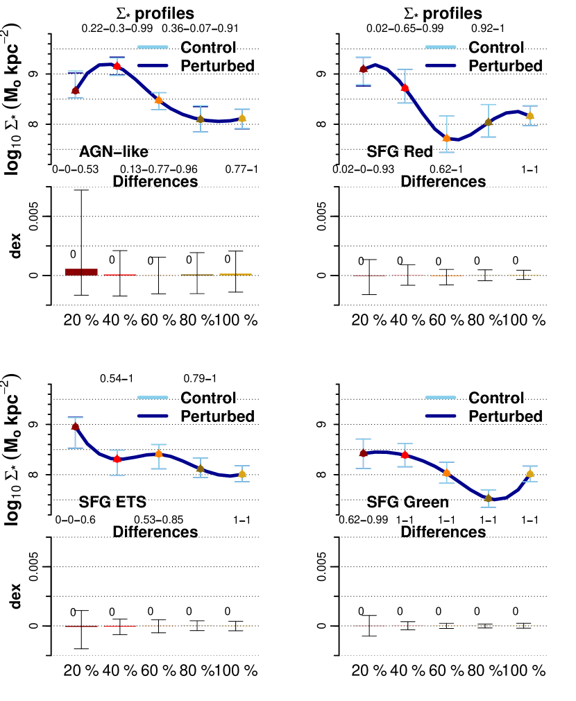
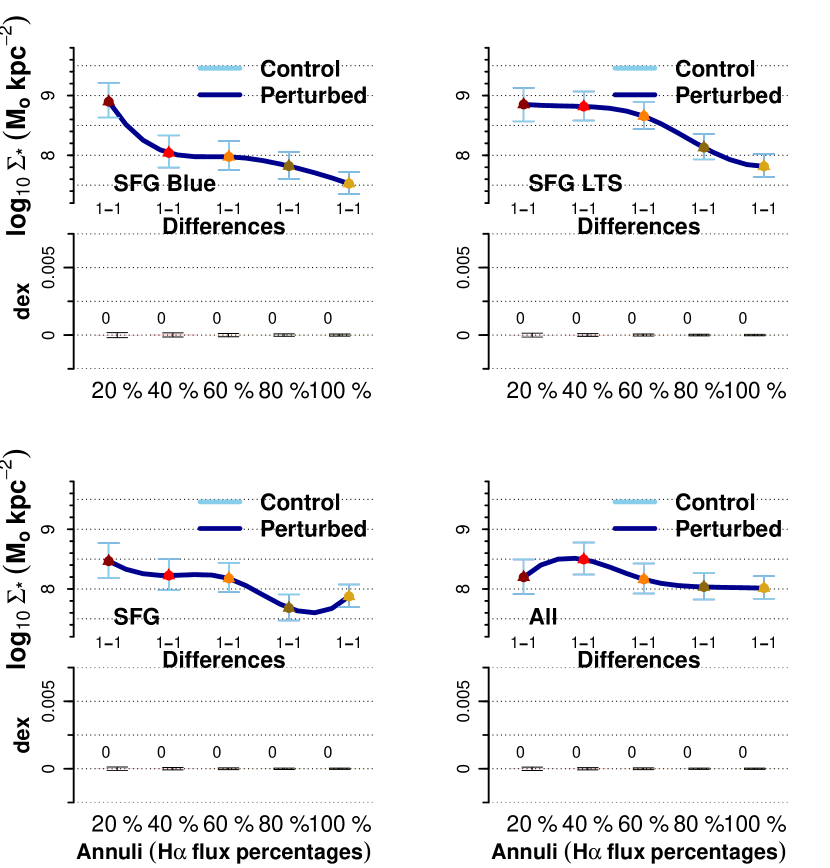
Figure 11: Annular profiles: $\mathrm{\Sigma}_{*}$. Throughout this work, all profiles use the amounts of annular star-forming regions per sample and subsample as in Fig. 5. Five consecutive-outward annuli denote the radial extension (see Section 3.5). “Differences” (bar heights by always subtracting the control values from the perturbed ones) are the medians of the annular distributions of differences (differences by pairing sample spaxels which are the closest in $\mathrm{\Sigma_{*}}$). Bar lines depict the interquartile ranges (IQRs, 1st to 3rd) of the distributions of differences. Symbols are both sample values giving each Difference. Symbol lines depict the IQRs of the annular distributions of each sample. Above and below the profiles, likelihoods from AD-permutation tests are found for each pair of sample distributions. Finally, a third statistics, Mann-Whitney (MW) test p-value, is given when at least one of the other two statistics results in a value lower than 0.5 (see text).

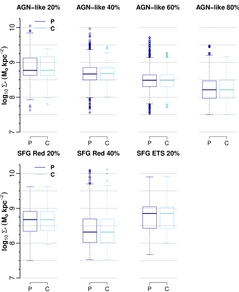
Figure 12: $\mathrm{\Sigma}_{*}$ distributions (P, perturbed, against C, control) for the annular cases of Fig. 11 in which at least one of the statistical tests results in a likelihood lower than 0.5.

Appendix C Resolved SFMSs

The annular comparison sets are shown in Table LABEL:tab:C1. It lists the linear regression coefficients of control and tA to tJ samples all on the SFMS plane. In each set, slopes marked with * are the closest ones to the slopes which result from the data in the respective set. Only significance difference tests (SDTs, see Section 4.1) with values above the statistical level are considered for this and that slope with the highest test value is marked (see Section 5.4). The criterion is that slopes are suggested to be different when the SDT value falls below the statistical level. Only these cases of different slopes are considered for comparisons (see Section 4.1). At last, from the K-S/Peacock two-sample test, $\mathrm{D_{2DKS}}$ differences marked with * reject the null hypothesis of a parent distribution as the origin.

Table 8: Comparison annular sets: control (C) and perturbed galaxies (tA-tJ, see text) on the SFMS plane. Linear regression slope (s) and intercept (i, M_⊙ yr^-1 kpc^-2) both with standard error (e). All models are statistically significant but two for control galaxies in the AGN-like sets (20 % annulus, 3rd and 4th from left to right). Slopes with * are the closest to the ones if combining both sample data. Significance difference tests (SDTs) per pair of slopes are shown too. $\mathrm{D_{2DKS}}$ differences (the maximum absolute ones between cumulative probability distributions, Peacock 1983, Yuanhui 2017) with * suggest that both distribution functions come from different parent ones. Finally, numbers of paired star-forming regions with annular totals at the very left (see Fig. 5).

	C	tA	C	tB	C	tC	C	tD	C	tE	C	tF	C	tG	C	tH	C	tI	C	tJ
	AGN-like
20 % s	$-$0.24	$-$1.18	$-$0.43	$-$1.16	$-$0.10	$-$0.99	$-$0.12	$-$1.38*	$-$0.29	$-$1.02	$-$0.24	$-$1.29	$-$0.53	$-$1.45	$-$0.25	$-$1.19	$-$0.33	$-$1.14	$-$0.31	$-$1.00
e	$-$0.09	$-$0.07	$-$0.11	$-$0.09	$-$0.14	$-$0.10	$-$0.22	$-$0.12	$-$0.07	$-$0.06	$-$0.08	$-$0.06	$-$0.15	$-$0.15	$-$0.08	$-$0.07	$-$0.08	$-$0.06	$-$0.06	$-$0.05
i	$-$3.61	$-$12.00	$-$5.31	$-$11.77	$-$2.34	$-$10.22	$-$0.36	$-$13.79	$-$4.05	$-$10.45	$-$3.63	$-$12.85	$-$6.20	$-$14.33	$-$3.70	$-$12.11	$-$4.44	$-$11.57	$-$4.20	$-$10.44
e	$-$0.76	$-$0.61	$-$0.95	$-$0.82	$-$1.29	$-$0.88	$-$1.99	$-$1.13	$-$0.65	$-$0.51	$-$0.66	$-$0.52	$-$1.29	$-$1.32	$-$0.75	$-$0.59	$-$0.67	$-$0.51	$-$0.55	$-$0.47
SDT	$-$0.00		$-$0.00		$-$0.00		$-$0.00		$-$0.00		$-$0.00		$-$0.00		$-$0.00		$-$0.00		$-$0.00
D2DKS	$-$0.37*		$-$0.15		$-$0.56*		$-$0.61*		$-$0.19		$-$0.22*		$-$0.26		$-$0.37*		$-$0.20*		$-$0.40*
1505	138		168		94		66		146		197		78		142		219		257
40 % s	$-$0.38	$-$1.10	$-$0.47	$-$0.65*	$-$0.29	$-$1.23	$-$0.42	$-$0.64*	$-$0.32	$-$1.16	$-$0.38	$-$1.01	$-$0.41	$-$1.17	$-$0.39	$-$1.00	$-$0.43	$-$0.56*	$-$0.44	$-$0.57*
e	$-$0.04	$-$0.06	$-$0.06	$-$0.10	$-$0.05	$-$0.07	$-$0.06	$-$0.08	$-$0.05	$-$0.07	$-$0.04	$-$0.05	$-$0.06	$-$0.10	$-$0.04	$-$0.05	$-$0.05	$-$0.07	$-$0.04	$-$0.06
i	$-$4.96	$-$11.17	$-$5.75	$-$7.30	$-$4.20	$-$12.31	$-$5.29	$-$7.12	$-$4.47	$-$11.60	$-$4.96	$-$10.19	$-$5.27	$-$11.56	$-$5.03	$-$10.20	$-$5.37	$-$6.54	$-$5.48	$-$6.47
e	$-$0.34	$-$0.52	$-$0.55	$-$0.82	$-$0.46	$-$0.66	$-$0.52	$-$0.74	$-$0.41	$-$0.64	$-$0.35	$-$0.46	$-$0.48	$-$0.86	$-$0.32	$-$0.47	$-$0.44	$-$0.60	$-$0.36	$-$0.52
SDT	$-$0.00		$-$0.11		$-$0.00		$-$0.04		$-$0.00		$-$0.00		$-$0.00		$-$0.00		$-$0.12		$-$0.09
D2DKS	$-$0.20*		$-$0.19*		$-$0.26*		$-$0.22*		$-$0.47*		$-$0.34*		$-$0.35*		$-$0.19*		$-$0.14		$-$0.24*
2961	360		214		267		236		116		297		262		404		311		494
60 % s	$-$0.82	$-$0.87*	$-$0.60	$-$0.22*	$-$0.91	$-$1.00*	$-$0.46	$-$0.45*	$-$0.90	$-$0.91*	$-$0.81	$-$0.83*	$-$0.61	$-$0.64*	$-$0.79	$-$0.85*	$-$0.61	$-$0.41*	$-$0.55	$-$0.37*
e	$-$0.04	$-$0.05	$-$0.07	$-$0.01	$-$0.04	$-$0.05	$-$0.06	$-$0.07	$-$0.05	$-$0.06	$-$0.04	$-$0.05	$-$0.06	$-$0.10	$-$0.04	$-$0.05	$-$0.06	$-$0.07	$-$0.04	$-$0.06
i	$-$8.78	$-$9.03	$-$6.96	$-$3.74	$-$9.62	$-$10.25	$-$5.82	$-$5.56	$-$9.47	$-$9.38	$-$8.68	$-$8.66	$-$6.99	$-$6.96	$-$8.56	$-$8.93	$-$6.99	$-$5.24	$-$6.55	$-$4.92
e	$-$0.34	$-$0.44	$-$0.55	$-$0.82	$-$0.38	$-$0.47	$-$0.48	$-$0.57	$-$0.39	$-$0.52	$-$0.34	$-$0.43	$-$0.49	$-$0.86	$-$0.33	$-$0.42	$-$0.48	$-$0.59	$-$0.37	$-$0.50
SDT	$-$0.47		$-$0.00		$-$0.21		$-$0.90		$-$0.96		$-$0.78		$-$0.82		$-$0.34		$-$0.03		$-$0.02
D2DKS	$-$0.21*		$-$0.16		$-$0.19*		$-$0.28*		$-$0.29*		$-$0.21*		$-$0.38*		$-$0.20*		$-$0.17*		$-$0.27*
4096	522		251		423		375		203		423		350		585		349		615
80 % s	$-$0.68	$-$0.87*	$-$0.51	$-$0.34*	$-$0.64	$-$0.87	$-$0.55*	$-$0.77	$-$0.70	$-$0.96*	$-$0.63	$-$0.89	$-$0.52	$-$0.30*	$-$0.66	$-$0.88	$-$0.49*	$-$0.38	$-$0.53*	$-$0.52
e	$-$0.04	$-$0.04	$-$0.06	$-$0.06	$-$0.04	$-$0.04	$-$0.05	$-$0.05	$-$0.05	$-$0.05	$-$0.04	$-$0.04	$-$0.06	$-$0.07	$-$0.04	$-$0.04	$-$0.07	$-$0.07	$-$0.05	$-$0.05
i	$-$7.65	$-$9.00	$-$6.23	$-$4.81	$-$7.24	$-$8.98	$-$6.51	$-$8.12	$-$7.80	$-$9.74	$-$7.23	$-$9.13	$-$6.28	$-$4.41	$-$7.47	$-$9.09	$-$6.02	$-$5.15	$-$6.40	$-$6.22
e	$-$0.30	$-$0.32	$-$0.52	$-$0.52	$-$0.35	$-$0.37	$-$0.41	$-$0.39	$-$0.40	$-$0.45	$-$0.31	$-$0.31	$-$0.47	$-$0.54	$-$0.31	$-$0.31	$-$0.56	$-$0.54	$-$0.38	$-$0.37
SDT	$-$0.00		$-$0.06		$-$0.00		$-$0.00		$-$0.00		$-$0.00		$-$0.02		$-$0.00		$-$0.26		$-$0.87
D2DKS	$-$0.25*		$-$0.14*		$-$0.18*		$-$0.30*		$-$0.22*		$-$0.20*		$-$0.20*		$-$0.22*		$-$0.10		$-$0.15*
5167	656		443		441		429		362		626		429		692		340		749
100 % s	$-$0.86	$-$0.69*	$-$0.92	$-$0.66*	$-$0.94	$-$0.62	$-$0.78	$-$0.60*	$-$0.91	$-$0.66*	$-$1.07	$-$0.77	$-$0.79	$-$0.37	$-$0.92	$-$0.72*	$-$0.87	$-$0.53*	$-$0.94	$-$0.59
e	$-$0.05	$-$0.05	$-$0.07	$-$0.09	$-$0.05	$-$0.06	$-$0.06	$-$0.06	$-$0.06	$-$0.06	$-$0.05	$-$0.06	$-$0.06	$-$0.07	$-$0.05	$-$0.05	$-$0.08	$-$0.09	$-$0.05	$-$0.06
i	$-$8.97	$-$7.59	$-$9.41	$-$7.38	$-$9.60	$-$7.01	$-$8.35	$-$6.74	$-$9.34	$-$7.36	$-$10.59	$-$8.21	$-$8.44	$-$4.90	$-$9.41	$-$7.76	$-$9.02	$-$6.37	$-$9.62	$-$6.72
e	$-$0.38	$-$0.38	$-$0.59	$-$0.69	$-$0.42	$-$0.46	$-$0.44	$-$0.46	$-$0.45	$-$0.49	$-$0.44	$-$0.44	$-$0.47	$-$0.56	$-$0.41	$-$0.41	$-$0.64	$-$0.75	$-$0.42	$-$0.45
SDT	$-$0.01		$-$0.02		$-$0.00		$-$0.02		$-$0.00		$-$0.00		$-$0.00		$-$0.00		$-$0.01		$-$0.00
D2DKS	$-$0.13*		$-$0.17*		$-$0.17*		$-$0.21*		$-$0.16*		$-$0.13*		$-$0.21*		$-$0.13*		$-$0.18*		$-$0.13*
4547	572		315		429		406		439		604		354		565		252		611
	SFG Red
20 % s	$-$0.77	$-$0.94*	$-$0.81	$-$0.90*	$-$0.76*	$-$0.95	$-$0.80	$-$0.90*	$-$0.80	$-$0.91*	$-$0.60	$-$0.87	$-$0.84	$-$0.72*	$-$0.82	$-$0.65*	$-$0.82	$-$0.57	$-$0.55	$-$0.92
e	$-$0.04	$-$0.04	$-$0.04	$-$0.04	$-$0.04	$-$0.04	$-$0.04	$-$0.04	$-$0.04	$-$0.04	$-$0.03	$-$0.03	$-$0.04	$-$0.04	$-$0.03	$-$0.04	$-$0.03	$-$0.04	$-$0.03	$-$0.03
i	$-$8.11	$-$9.48	$-$8.41	$-$9.12	$-$7.98	$-$9.54	$-$8.34	$-$9.12	$-$8.31	$-$9.22	$-$6.57	$-$8.97	$-$8.69	$-$7.73	$-$8.47	$-$7.11	$-$8.46	$-$6.36	$-$6.17	$-$9.34
e	$-$0.33	$-$0.33	$-$0.34	$-$0.34	$-$0.35	$-$0.34	$-$0.33	$-$0.33	$-$0.32	$-$0.31	$-$0.22	$-$0.25	$-$0.31	$-$0.39	$-$0.30	$-$0.38	$-$0.29	$-$0.35	$-$0.22	$-$0.24
SDT	$-$0.00		$-$0.10		$-$0.00		$-$0.06		$-$0.03		$-$0.00		$-$0.03		$-$0.00		$-$0.00		$-$0.00
D2DKS	$-$0.19*		$-$0.16*		$-$0.20*		$-$0.17*		$-$0.17*		$-$0.29*		$-$0.16*		$-$0.11*		$-$0.11*		$-$0.25*
6344	565		588		531		613		603		660		620		636		718		810
40 % s	$-$0.89*	$-$0.84	$-$0.88*	$-$0.80	$-$0.87*	$-$0.87	$-$0.89*	$-$0.77	$-$0.87*	$-$0.81	$-$0.84	$-$1.04	$-$1.06	$-$0.67	$-$0.92	$-$0.65	$-$0.94	$-$0.62	$-$0.76	$-$0.94
e	$-$0.03	$-$0.03	$-$0.03	$-$0.03	$-$0.03	$-$0.03	$-$0.03	$-$0.03	$-$0.03	$-$0.03	$-$0.04	$-$0.04	$-$0.04	$-$0.05	$-$0.03	$-$0.03	$-$0.03	$-$0.03	$-$0.04	$-$0.03
i	$-$9.04	$-$8.48	$-$8.97	$-$8.20	$-$8.89	$-$8.73	$-$9.11	$-$7.98	$-$8.89	$-$8.31	$-$8.61	$-$10.25	$-$10.56	$-$7.15	$-$9.29	$-$6.99	$-$9.44	$-$6.71	$-$7.97	$-$9.35
e	$-$0.27	$-$0.24	$-$0.26	$-$0.26	$-$0.28	$-$0.25	$-$0.26	$-$0.26	$-$0.27	$-$0.26	$-$0.32	$-$0.33	$-$0.34	$-$0.43	$-$0.24	$-$0.23	$-$0.24	$-$0.24	$-$0.30	$-$0.27
SDT	$-$0.25		$-$0.07		$-$0.97		$-$0.01		$-$0.21		$-$0.00		$-$0.00		$-$0.00		$-$0.00		$-$0.00
D2DKS	$-$0.18*		$-$0.15*		$-$0.18*		$-$0.15*		$-$0.15*		$-$0.17*		$-$0.12		$-$0.16*		$-$0.18*		$-$0.22*
6638	739		763		706		789		778		385		438		740		669		631
60 % s	$-$0.84	$-$0.99	$-$0.86	$-$0.94*	$-$0.84	$-$0.99*	$-$0.85	$-$0.93*	$-$0.85	$-$0.93*	$-$0.87	$-$1.22	$-$0.86	$-$0.99*	$-$0.85	$-$0.83*	$-$0.85	$-$0.82*	$-$0.83	$-$1.00*
e	$-$0.03	$-$0.03	$-$0.03	$-$0.03	$-$0.03	$-$0.03	$-$0.03	$-$0.03	$-$0.03	$-$0.03	$-$0.05	$-$0.05	$-$0.05	$-$0.06	$-$0.03	$-$0.03	$-$0.03	$-$0.03	$-$0.04	$-$0.04
i	$-$8.64	$-$9.78	$-$8.77	$-$9.38	$-$8.63	$-$9.76	$-$8.74	$-$9.30	$-$8.75	$-$9.35	$-$8.87	$-$11.71	$-$8.78	$-$9.91	$-$8.72	$-$8.48	$-$8.71	$-$8.36	$-$8.53	$-$9.83
e	$-$0.25	$-$0.25	$-$0.24	$-$0.26	$-$0.27	$-$0.27	$-$0.24	$-$0.25	$-$0.26	$-$0.27	$-$0.39	$-$0.39	$-$0.43	$-$0.49	$-$0.24	$-$0.25	$-$0.24	$-$0.26	$-$0.30	$-$0.30
SDT	$-$0.00		$-$0.06		$-$0.00		$-$0.08		$-$0.09		$-$0.00		$-$0.08		$-$0.54		$-$0.40		$-$0.00
D2DKS	$-$0.14*		$-$0.12*		$-$0.12*		$-$0.11*		$-$0.10*		$-$0.17*		$-$0.10		$-$0.12*		$-$0.13*		$-$0.18*
7430	825		902		800		932		886		352		500		824		757		652
80 % s	$-$0.85	$-$1.10	$-$0.85	$-$1.11	$-$0.83	$-$1.06	$-$0.86	$-$1.10	$-$0.83	$-$1.07	$-$0.84	$-$1.31	$-$0.99	$-$1.01*	$-$0.91	$-$0.88*	$-$0.92	$-$0.89*	$-$0.85	$-$1.15
e	$-$0.03	$-$0.03	$-$0.03	$-$0.04	$-$0.03	$-$0.04	$-$0.03	$-$0.04	$-$0.03	$-$0.04	$-$0.05	$-$0.05	$-$0.04	$-$0.05	$-$0.03	$-$0.03	$-$0.03	$-$0.03	$-$0.04	$-$0.04
i	$-$8.68	$-$10.71	$-$8.73	$-$10.75	$-$8.51	$-$10.40	$-$8.77	$-$10.66	$-$8.51	$-$10.45	$-$8.63	$-$12.40	$-$9.89	$-$10.05	$-$9.22	$-$8.98	$-$9.26	$-$8.99	$-$8.67	$-$11.02
e	$-$0.24	$-$0.28	$-$0.24	$-$0.29	$-$0.26	$-$0.30	$-$0.24	$-$0.29	$-$0.25	$-$0.31	$-$0.38	$-$0.42	$-$0.32	$-$0.43	$-$0.22	$-$0.28	$-$0.22	$-$0.29	$-$0.30	$-$0.34
SDT	$-$0.00		$-$0.00		$-$0.00		$-$0.00		$-$0.00		$-$0.00		$-$0.77		$-$0.47		$-$0.47		$-$0.00
D2DKS	$-$0.12*		$-$0.12*		$-$0.12*		$-$0.12*		$-$0.12*		$-$0.19*		$-$0.12*		$-$0.09		$-$0.09		$-$0.14*
7234	758		866		768		880		853		377		667		760		772		533
100 % s	$-$0.70	$-$1.08	$-$0.65	$-$0.96	$-$0.64	$-$1.00	$-$0.70	$-$1.01	$-$0.64	$-$0.98	$-$0.73	$-$1.25	$-$0.71	$-$0.49*	$-$0.74	$-$0.39	$-$0.71	$-$0.42	$-$0.76	$-$1.09*
e	$-$0.05	$-$0.06	$-$0.04	$-$0.06	$-$0.05	$-$0.06	$-$0.05	$-$0.06	$-$0.05	$-$0.06	$-$0.06	$-$0.08	$-$0.04	$-$0.05	$-$0.04	$-$0.05	$-$0.04	$-$0.05	$-$0.06	$-$0.08
i	$-$7.54	$-$10.44	$-$7.14	$-$9.51	$-$7.04	$-$9.80	$-$7.56	$-$9.95	$-$7.08	$-$9.72	$-$7.80	$-$11.85	$-$7.63	$-$5.90	$-$7.89	$-$5.04	$-$7.66	$-$5.26	$-$8.07	$-$10.53
e	$-$0.38	$-$0.51	$-$0.35	$-$0.47	$-$0.40	$-$0.52	$-$0.36	$-$0.50	$-$0.38	$-$0.50	$-$0.52	$-$0.67	$-$0.33	$-$0.41	$-$0.32	$-$0.42	$-$0.31	$-$0.42	$-$0.47	$-$0.63
SDT	$-$0.00		$-$0.00		$-$0.00		$-$0.00		$-$0.00		$-$0.00		$-$0.00		$-$0.00		$-$0.00		$-$0.00
D2DKS	$-$0.25*		$-$0.23*		$-$0.26*		$-$0.22*		$-$0.24*		$-$0.27*		$-$0.12*		$-$0.13*		$-$0.13*		$-$0.29*
6681	606		741		622		727		727		461		876		719		778		424
	SFG ETS
20 % s	$-$0.64	$-$1.09	$-$0.90*	$-$0.95	$-$0.69	$-$1.01	$-$0.80	$-$1.04	$-$0.88*	$-$0.97	$-$0.80	$-$1.06	$-$0.80*	$-$0.69	$-$0.68	$-$1.01	$-$0.81*	$-$0.90	$-$0.81	$-$1.13
e	$-$0.04	$-$0.03	$-$0.04	$-$0.03	$-$0.03	$-$0.03	$-$0.03	$-$0.03	$-$0.04	$-$0.03	$-$0.04	$-$0.03	$-$0.04	$-$0.03	$-$0.04	$-$0.03	$-$0.04	$-$0.03	$-$0.03	$-$0.03
i	$-$7.05	$-$10.94	$-$9.35	$-$-9.79	$-$7.47	$-$10.26	$-$8.41	$-$10.59	$-$9.16	$-$9.97	$-$8.43	$-$10.71	$-$8.44	$-$7.40	$-$7.41	$-$10.32	$-$8.56	$-$9.28	$-$8.53	$-$11.30
e	$-$0.32	$-$0.27	$-$0.31	$-$0.26	$-$0.30	$-$0.23	$-$0.28	$-$0.23	$-$0.31	$-$0.25	$-$0.32	$-$0.25	$-$0.37	$-$0.29	$-$0.31	$-$0.25	$-$0.34	$-$0.28	$-$0.30	$-$0.23
SDT	$-$0.00		$-$0.26		$-$0.00		$-$0.00		$-$0.04		$-$0.00		$-$0.04		$-$0.00		$-$0.08		$-$0.00
D2DKS	$-$0.23*		$-$0.15*		$-$0.18*		$-$0.14*		$-$0.15*		$-$0.16*		$-$0.19*		$-$0.19*		$-$0.18*		$-$0.18*
8756	790		940		1033		1015		923		774		798		859		800		824
40 % s	$-$0.46	$-$1.09	$-$0.56	$-$1.04	$-$0.40	$-$0.92	$-$0.51	$-$1.06	$-$0.54	$-$1.00	$-$0.50	$-$1.11	$-$0.56	$-$0.90	$-$0.36	$-$1.08	$-$0.63	$-$1.03	$-$0.48	$-$1.18
e	$-$0.03	$-$0.03	$-$0.03	$-$0.03	$-$0.03	$-$0.03	$-$0.03	$-$0.03	$-$0.03	$-$0.03	$-$0.03	$-$0.03	$-$0.05	$-$0.04	$-$0.03	$-$0.03	$-$0.04	$-$0.04	$-$0.03	$-$0.02
i	$-$5.44	$-$10.83	$-$6.29	$-$10.37	$-$4.96	$-$9.38	$-$5.89	$-$10.57	$-$6.15	$-$10.07	$-$5.75	$-$10.97	$-$6.35	$-$9.19	$-$4.63	$-$10.77	$-$6.91	$-$10.29	$-$5.66	$-$11.57
e	$-$0.27	$-$0.24	$-$0.27	$-$0.24	$-$0.24	$-$0.22	$-$0.26	$-$0.22	$-$0.28	$-$0.25	$-$0.28	$-$0.24	$-$0.40	$-$0.39	$-$0.26	$-$0.23	$-$0.37	$-$0.31	$-$0.28	$-$0.21
SDT	$-$0.00		$-$0.00		$-$0.00		$-$0.00		$-$0.00		$-$0.00		$-$0.00		$-$0.00		$-$0.00		$-$0.00
D2DKS	$-$0.18*		$-$0.20*		$-$0.18*		$-$0.17*		$-$0.18*		$-$0.20*		$-$0.21*		$-$0.20*		$-$0.23*		$-$0.23*
11563	1120		1236		1521		1348		1189		1113		857		1246		841		1092
60 % s	$-$0.47	$-$1.14	$-$0.62	$-$1.10	$-$0.36	$-$0.89	$-$0.66	$-$1.06	$-$0.67	$-$1.13	$-$0.68	$-$1.07	$-$0.87*	$-$1.01	$-$0.51	$-$1.08	$-$0.80	$-$1.18	$-$0.67	$-$1.14
e	$-$0.04	$-$0.03	$-$0.04	$-$0.03	$-$0.03	$-$0.02	$-$0.03	$-$0.02	$-$0.04	$-$0.03	$-$0.04	$-$0.03	$-$0.06	$-$0.05	$-$0.04	$-$0.03	$-$0.04	$-$0.03	$-$0.03	$-$0.02
i	$-$5.58	$-$11.13	$-$6.77	$-$10.79	$-$4.71	$-$9.07	$-$7.11	$-$10.49	$-$7.22	$-$11.09	$-$7.32	$-$10.55	$-$8.92	$-$10.12	$-$5.89	$-$10.70	$-$8.39	$-$11.52	$-$7.21	$-$11.13
e	$-$0.33	$-$0.23	$-$0.29	$-$0.22	$-$0.28	$-$0.20	$-$0.29	$-$0.21	$-$0.33	$-$0.25	$-$0.30	$-$0.24	$-$0.48	$-$0.44	$-$0.30	$-$0.23	$-$0.37	$-$0.28	$-$0.29	$-$0.19
SDT	$-$0.00		$-$0.00		$-$0.00		$-$0.00		$-$0.00		$-$0.00		$-$0.06		$-$0.00		$-$0.00		$-$0.00
D2DKS	$-$0.13*		$-$0.10*		$-$0.13*		$-$0.10*		$-$0.10*		$-$0.09*		$-$0.09		$-$0.12*		$-$0.13*		$-$0.10*
13093	1191		1499		1750		1593		1347		1171		927		1334		995		1286
80 % s	$-$1.10*	$-$1.22	$-$1.06*	$-$1.15	$-$0.99*	$-$0.95	$-$1.09*	$-$1.17	$-$1.05*	$-$1.16	$-$1.06*	$-$1.21	$-$1.02	$-$1.19*	$-$1.04*	$-$1.18	$-$1.11*	$-$1.13	$-$1.08*	$-$1.18
e	$-$0.03	$-$0.03	$-$0.03	$-$0.03	$-$0.03	$-$0.03	$-$0.03	$-$0.03	$-$0.03	$-$0.03	$-$0.03	$-$0.03	$-$0.04	$-$0.05	$-$0.03	$-$0.03	$-$0.04	$-$0.03	$-$0.03	$-$0.03
i	$-$10.85	$-$11.72	$-$10.50	$-$11.20	$-$9.94	$-$9.56	$-$10.72	$-$11.41	$-$10.43	$-$11.29	$-$10.52	$-$11.71	$-$10.15	$-$11.58	$-$10.30	$-$11.43	$-$10.89	$-$11.05	$-$10.69	$-$11.45
e	$-$0.27	$-$0.24	$-$0.24	$-$0.23	$-$0.23	$-$0.22	$-$0.24	$-$0.22	$-$0.27	$-$0.25	$-$0.26	$-$0.24	$-$0.37	$-$0.39	$-$0.26	$-$0.24	$-$0.29	$-$0.28	$-$0.24	$-$0.22
SDT	$-$0.01		$-$0.03		$-$0.27		$-$0.03		$-$0.02		$-$0.00		$-$0.01		$-$0.00		$-$0.63		$-$0.01
D2DKS	$-$0.09*		$-$0.10*		$-$0.10*		$-$0.10*		$-$0.11*		$-$0.07*		$-$0.15*		$-$0.07*		$-$0.10*		$-$0.08*
15352	1431		1730		1957		1928		1534		1310		1101		1458		1305		1598
100 % s	$-$0.87	$-$1.20	$-$0.78	$-$1.11	$-$0.68	$-$0.90	$-$0.80	$-$1.13	$-$0.72	$-$1.08	$-$0.78	$-$1.20	$-$0.68	$-$1.08	$-$0.78	$-$1.02	$-$0.79	$-$1.05	$-$0.78	$-$1.24
e	$-$0.04	$-$0.05	$-$0.04	$-$0.04	$-$0.04	$-$0.04	$-$0.04	$-$0.04	$-$0.04	$-$0.05	$-$0.04	$-$0.05	$-$0.04	$-$0.05	$-$0.04	$-$0.05	$-$0.04	$-$0.05	$-$0.04	$-$0.04
i	$-$8.93	$-$11.51	$-$8.20	$-$10.91	$-$7.44	$-$9.13	$-$8.36	$-$11.07	$-$7.79	$-$10.66	$-$8.20	$-$11.50	$-$7.44	$-$10.70	$-$8.20	$-$11.55	$-$8.31	$-$10.38	$-$8.27	$-$11.85
e	$-$0.35	$-$0.38	$-$0.29	$-$0.34	$-$0.31	$-$0.33	$-$0.29	$-$0.33	$-$0.32	$-$0.36	$-$0.34	$-$0.39	$-$0.36	$-$0.44	$-$0.33	$-$0.37	$-$0.34	$-$0.39	$-$0.34	$-$0.35
SDT	$-$0.00		$-$0.00		$-$0.00		$-$0.00		$-$0.00		$-$0.00		$-$0.00		$-$0.00		$-$0.00		$-$0.00
D2DKS	$-$0.10*		$-$0.10*		$-$0.08*		$-$0.09*		$-$0.10*		$-$0.14*		$-$0.12*		$-$0.14*		$-$0.10*		$-$0.12*
12397	1052		1405		1448		1532		1362		1056		1004		1192		1093		1253
	SFG Green
20 % s	$-$0.68	$-$0.86	$-$0.64	$-$0.75	$-$0.59	$-$0.70	$-$0.75	$-$0.73*	$-$0.67	$-$0.82	$-$0.66	$-$0.77	$-$0.60*	$-$0.62	$-$0.62	$-$0.78	$-$0.71	$-$0.86	$-$0.64	$-$0.78
e	$-$0.02	$-$0.02	$-$0.02	$-$0.01	$-$0.02	$-$0.02	$-$0.02	$-$0.02	$-$0.02	$-$0.02	$-$0.02	$-$0.02	$-$0.02	$-$0.02	$-$0.02	$-$0.02	$-$0.02	$-$0.02	$-$0.02	$-$0.02
i	$-$7.46	$-$8.89	$-$7.13	$-$7.96	$-$6.73	$-$7.50	$-$7.99	$-$7.77	$-$7.36	$-$8.54	$-$7.27	$-$8.06	$-$6.79	$-$6.84	$-$6.93	$-$8.24	$-$7.72	$-$8.87	$-$7.14	$-$8.17
e	$-$0.14	$-$0.13	$-$0.13	$-$0.13	$-$0.13	$-$0.13	$-$0.15	$-$0.17	$-$0.16	$-$0.14	$-$0.17	$-$0.14	$-$0.16	$-$0.13	$-$0.15	$-$0.14	$-$0.16	$-$0.14	$-$0.18	$-$0.19
SDT	$-$0.00		$-$0.00		$-$0.00		$-$0.62		$-$0.00		$-$0.00		$-$0.58		$-$0.00		$-$0.00		$-$0.00
D2DKS	$-$0.14*		$-$0.21*		$-$0.17*		$-$0.17*		$-$0.19*		$-$0.20*		$-$0.16*		$-$0.15*		$-$0.19*		$-$0.16*
21121	2374		2457		2632		2173		1873		2136		1813		2110		1694		1859
40 % s	$-$0.73	$-$0.86	$-$0.73	$-$0.73*	$-$0.70*	$-$0.64	$-$0.75	$-$0.70*	$-$0.76*	$-$0.86	$-$0.73	$-$0.84	$-$0.69	$-$0.57	$-$0.74*	$-$0.72	$-$0.73	$-$0.84	$-$0.74*	$-$0.73
e	$-$0.02	$-$0.02	$-$0.02	$-$0.02	$-$0.02	$-$0.02	$-$0.02	$-$0.02	$-$0.03	$-$0.02	$-$0.02	$-$0.02	$-$0.02	$-$0.02	$-$0.02	$-$0.02	$-$0.02	$-$0.02	$-$0.02	$-$0.02
i	$-$7.78	$-$8.90	$-$7.79	$-$7.74	$-$7.53	$-$6.98	$-$7.98	$-$7.44	$-$8.01	$-$8.84	$-$7.73	$-$8.64	$-$7.46	$-$6.50	$-$7.82	$-$7.71	$-$7.76	$-$8.69	$-$7.83	$-$7.76
e	$-$0.19	$-$0.18	$-$0.19	$-$0.18	$-$0.16	$-$0.15	$-$0.17	$-$0.17	$-$0.22	$-$0.20	$-$0.17	$-$0.15	$-$0.18	$-$0.15	$-$0.19	$-$0.17	$-$0.18	$-$0.14	$-$0.18	$-$0.18
SDT	$-$0.00		$-$0.98		$-$0.03		$-$0.05		$-$0.00		$-$0.00		$-$0.00		$-$0.56		$-$0.00		$-$0.90
D2DKS	$-$0.06*		$-$0.09*		$-$0.13*		$-$0.10*		$-$0.08*		$-$0.09*		$-$0.08*		$-$0.07*		$-$0.06		$-$0.08*
22530	2320		2428		2693		2522		2226		2205		1716		2179		1881		2360
60 % s	$-$0.73	$-$0.80*	$-$0.78	$-$0.73*	$-$0.75	$-$0.59	$-$0.78	$-$0.65	$-$0.81	$-$0.81*	$-$0.84	$-$0.79*	$-$0.80	$-$0.53	$-$0.79	$-$0.75*	$-$0.78*	$-$0.81	$-$0.78	$-$0.72*
e	$-$0.03	$-$0.03	$-$0.02	$-$0.02	$-$0.02	$-$0.02	$-$0.02	$-$0.02	$-$0.02	$-$0.02	$-$0.02	$-$0.02	$-$0.02	$-$0.03	$-$0.02	$-$0.02	$-$0.02	$-$0.02	$-$0.02	$-$0.02
i	$-$7.80	$-$8.31	$-$8.21	$-$7.76	$-$8.00	$-$6.60	$-$8.24	$-$7.04	$-$8.51	$-$8.47	$-$8.73	$-$8.22	$-$8.35	$-$6.14	$-$8.31	$-$7.97	$-$8.24	$-$8.39	$-$8.18	$-$7.67
e	$-$0.21	$-$0.24	$-$0.19	$-$0.19	$-$0.17	$-$0.18	$-$0.16	$-$0.18	$-$0.20	$-$0.20	$-$0.18	$-$0.18	$-$0.19	$-$0.21	$-$0.19	$-$0.19	$-$0.20	$-$0.19	$-$0.17	$-$0.18
SDT	$-$0.08		$-$0.14		$-$0.00		$-$0.00		$-$1.00		$-$0.08		$-$0.00		$-$0.22		$-$0.53		$-$0.07
D2DKS	$-$0.08*		$-$0.10*		$-$0.11*		$-$0.11*		$-$0.09*		$-$0.09*		$-$0.08*		$-$0.06		$-$0.07*		$-$0.07*
22614	2257		2522		2606		2691		2420		2081		1547		2090		1912		2488
80 % s	$-$0.77	$-$0.85*	$-$0.87	$-$0.81*	$-$0.78	$-$0.59	$-$0.83	$-$0.69	$-$0.90	$-$0.93*	$-$0.89	$-$0.92*	$-$0.82	$-$0.58	$-$0.86	$-$0.90*	$-$0.80	$-$0.69*	$-$0.80	$-$0.81*
e	$-$0.03	$-$0.03	$-$0.03	$-$0.03	$-$0.02	$-$0.03	$-$0.02	$-$0.03	$-$0.03	$-$0.03	$-$0.02	$-$0.03	$-$0.03	$-$0.03	$-$0.03	$-$0.03	$-$0.03	$-$0.03	$-$0.02	$-$0.03
i	$-$8.22	$-$8.76	$-$8.97	$-$8.40	$-$8.28	$-$6.63	$-$8.70	$-$7.47	$-$9.21	$-$9.40	$-$9.18	$-$9.30	$-$8.62	$-$6.63	$-$8.92	$-$9.18	$-$8.47	$-$7.48	$-$8.46	$-$8.42
e	$-$0.25	$-$0.26	$-$0.20	$-$0.21	$-$0.19	$-$0.21	$-$0.19	$-$0.20	$-$0.21	$-$0.22	$-$0.20	$-$0.21	$-$0.26	$-$0.26	$-$0.22	$-$0.23	$-$0.23	$-$0.23	$-$0.19	$-$0.21
SDT	$-$0.07		$-$0.11		$-$0.00		$-$0.00		$-$0.35		$-$0.53		$-$0.00		$-$0.26		$-$0.00		$-$0.92
D2DKS	$-$0.11*		$-$0.15*		$-$0.12*		$-$0.13*		$-$0.12*		$-$0.09*		$-$0.09*		$-$0.12*		$-$0.09*		$-$0.08*
22221	2247		2518		2592		2699		2373		2099		1406		1913		1878		2496
100 % s	$-$0.80	$-$0.59	$-$0.88	$-$0.74*	$-$0.83	$-$0.37	$-$0.87	$-$0.69	$-$0.88	$-$0.77*	$-$0.94	$-$0.83*	$-$0.85	$-$0.35	$-$0.88	$-$0.88*	$-$0.86	$-$0.41	$-$0.84	$-$0.82*
e	$-$0.04	$-$0.04	$-$0.03	$-$0.04	$-$0.03	$-$0.04	$-$0.03	$-$0.04	$-$0.03	$-$0.04	$-$0.04	$-$0.04	$-$0.04	$-$0.05	$-$0.04	$-$0.04	$-$0.04	$-$0.04	$-$0.04	$-$0.04
i	$-$8.40	$-$6.70	$-$9.08	$-$7.97	$-$8.67	$-$5.03	$-$8.94	$-$7.53	$-$9.03	$-$8.19	$-$9.51	$-$8.60	$-$8.77	$-$4.93	$-$9.07	$-$9.01	$-$8.92	$-$5.35	$-$8.74	$-$8.52
e	$-$0.32	$-$0.33	$-$0.27	$-$0.30	$-$0.27	$-$0.29	$-$0.26	$-$0.29	$-$0.27	$-$0.29	$-$0.28	$-$0.33	$-$0.32	$-$0.36	$-$0.29	$-$0.34	$-$0.32	$-$0.34	$-$0.29	$-$0.31
SDT	$-$0.00		$-$0.01		$-$0.00		$-$0.00		$-$0.03		$-$0.04		$-$0.00		$-$0.97		$-$0.00		$-$0.68
D2DKS	$-$0.09*		$-$0.08*		$-$0.08*		$-$0.08*		$-$0.09*		$-$0.06		$-$0.14*		$-$0.07		$-$0.10*		$-$0.07*
15604	1619		1741		1662		1768		1758		1250		1096		1460		1455		1795
	SFG Blue
20 % s	$-$1.03*	$-$0.97	$-$1.00	$-$0.83	$-$1.02*	$-$0.99	$-$1.03	$-$0.87	$-$1.04	$-$0.91	$-$1.05	$-$0.95	$-$1.05	$-$0.99*	$-$1.04	$-$0.90	$-$1.03	$-$0.95	$-$1.02	$-$0.90
e	$-$0.01	$-$0.01	$-$0.01	$-$0.01	$-$0.01	$-$0.01	$-$0.02	$-$0.01	$-$0.02	$-$0.02	$-$0.02	$-$0.02	$-$0.01	$-$0.01	$-$0.02	$-$0.01	$-$0.01	$-$0.01	$-$0.01	$-$0.01
i	$-$10.39	$-$9.88	$-$10.11	$-$8.71	$-$10.31	$-$9.97	$-$10.37	$-$9.00	$-$10.47	$-$9.36	$-$10.55	$-$9.74	$-$10.54	$-$10.10	$-$10.48	$-$9.25	$-$10.39	$-$9.73	$-$10.34	$-$9.26
e	$-$0.13	$-$0.12	$-$0.11	$-$0.11	$-$0.13	$-$0.12	$-$0.13	$-$0.12	$-$0.14	$-$0.15	$-$0.13	$-$0.13	$-$0.13	$-$0.13	$-$0.13	$-$0.13	$-$0.11	$-$0.11	$-$0.12	$-$0.11
SDT	$-$0.01		$-$0.00		$-$0.10		$-$0.00		$-$0.00		$-$0.00		$-$0.01		$-$0.00		$-$0.00		$-$0.00
D2DKS	$-$0.06*		$-$0.07*		$-$0.07*		$-$0.10*		$-$0.07*		$-$0.06*		$-$0.05		$-$0.07*		$-$0.06*		$-$0.07*
30121	2687		3259		2983		2560		2412		3108		3075		2848		3694		3495
40 % s	$-$1.05	$-$0.97	$-$1.04	$-$0.88	$-$1.05	$-$0.93	$-$1.05	$-$0.90	$-$1.07	$-$0.93	$-$1.08	$-$0.84	$-$1.07	$-$0.91	$-$1.05	$-$0.90	$-$1.06	$-$0.88	$-$1.02	$-$0.88
e	$-$0.01	$-$0.01	$-$0.01	$-$0.01	$-$0.01	$-$0.01	$-$0.02	$-$0.02	$-$0.02	$-$0.01	$-$0.01	$-$0.01	$-$0.01	$-$0.01	$-$0.01	$-$0.01	$-$0.01	$-$0.01	$-$0.01	$-$0.01
i	$-$10.40	$-$9.78	$-$10.35	$-$9.02	$-$10.38	$-$9.38	$-$10.36	$-$9.19	$-$10.58	$-$9.42	$-$10.66	$-$8.71	$-$10.59	$-$9.27	$-$10.42	$-$9.21	$-$10.50	$-$8.99	$-$10.17	$-$8.99
e	$-$0.12	$-$0.11	$-$0.12	$-$0.12	$-$0.12	$-$0.11	$-$0.14	$-$0.13	$-$0.13	$-$0.12	$-$0.12	$-$0.11	$-$0.12	$-$0.12	$-$0.12	$-$0.11	$-$0.11	$-$0.10	$-$0.12	$-$0.11
SDT	$-$0.00		$-$0.00		$-$0.00		$-$0.00		$-$0.00		$-$0.00		$-$0.00		$-$0.00		$-$0.00		$-$0.00
D2DKS	$-$0.08*		$-$0.10*		$-$0.07*		$-$0.09*		$-$0.09*		$-$0.09*		$-$0.10*		$-$0.10*		$-$0.07*		$-$0.09*
37126	3676		3055		4016		2926		3565		4143		4022		3944		4287		3492
60 % s	$-$1.00	$-$0.87	$-$1.02	$-$0.87	$-$1.01*	$-$0.94	$-$1.01	$-$0.87	$-$1.03	$-$0.93	$-$1.04	$-$0.80	$-$1.01	$-$0.86	$-$1.00	$-$0.84	$-$1.02	$-$0.86	$-$1.02	$-$0.89
e	$-$0.01	$-$0.02	$-$0.01	$-$0.02	$-$0.01	$-$0.01	$-$0.02	$-$0.02	$-$0.02	$-$0.02	$-$0.01	$-$0.02	$-$0.01	$-$0.02	$-$0.01	$-$0.02	$-$0.01	$-$0.01	$-$0.01	$-$0.02
i	$-$9.93	$-$8.91	$-$10.08	$-$8.88	$-$10.03	$-$9.40	$-$10.04	$-$8.86	$-$10.17	$-$9.41	$-$10.25	$-$8.31	$-$10.00	$-$8.87	$-$9.97	$-$8.70	$-$10.07	$-$8.78	$-$10.11	$-$9.06
e	$-$0.11	$-$0.13	$-$0.12	$-$0.14	$-$0.12	$-$0.12	$-$0.13	$-$0.13	$-$0.12	$-$0.14	$-$0.12	$-$0.13	$-$0.12	$-$0.13	$-$0.11	$-$0.12	$-$0.11	$-$0.12	$-$0.12	$-$0.13
SDT	$-$0.00		$-$0.00		$-$0.00		$-$0.00		$-$0.00		$-$0.00		$-$0.00		$-$0.00		$-$0.00		$-$0.00
D2DKS	$-$0.06*		$-$0.07*		$-$0.09*		$-$0.06*		$-$0.05*		$-$0.08*		$-$0.06*		$-$0.07*		$-$0.06*		$-$0.06*
39820	4115		3091		4536		3526		3641		4021		4029		4327		4551		3983
80 % s	$-$0.92	$-$0.91*	$-$0.92	$-$0.86*	$-$0.91*	$-$0.97	$-$0.88*	$-$0.84	$-$0.89	$-$0.90*	$-$0.89	$-$0.84*	$-$0.89	$-$0.88*	$-$0.89	$-$0.86*	$-$0.90	$-$0.91*	$-$0.90	$-$0.90*
e	$-$0.01	$-$0.02	$-$0.02	$-$0.02	$-$0.02	$-$0.02	$-$0.02	$-$0.02	$-$0.02	$-$0.02	$-$0.02	$-$0.02	$-$0.02	$-$0.02	$-$0.01	$-$0.02	$-$0.01	$-$0.01	$-$0.01	$-$0.02
i	$-$9.29	$-$9.19	$-$9.26	$-$8.79	$-$9.19	$-$9.67	$-$8.95	$-$8.72	$-$9.08	$-$9.10	$-$9.04	$-$8.68	$-$9.05	$-$9.02	$-$9.04	$-$8.83	$-$9.09	$-$9.25	$-$9.16	$-$9.13
e	$-$0.12	$-$0.13	$-$0.13	$-$0.14	$-$0.12	$-$0.12	$-$0.13	$-$0.13	$-$0.14	$-$0.15	$-$0.13	$-$0.14	$-$0.13	$-$0.14	$-$0.12	$-$0.12	$-$0.11	$-$0.12	$-$0.12	$-$0.12
SDT	$-$0.54		$-$0.01		$-$0.00		$-$0.15		$-$0.86		$-$0.05		$-$0.75		$-$0.14		$-$0.37		$-$0.67
D2DKS	$-$0.04*		$-$0.05*		$-$0.05*		$-$0.07*		$-$0.03		$-$0.06*		$-$0.07*		$-$0.07*		$-$0.05*		$-$0.06*
45321	4695		3661		4948		4402		4039		4428		4431		4907		5039		4771
100 % s	$-$0.80	$-$0.84*	$-$0.79	$-$0.80*	$-$0.78	$-$1.01	$-$0.83	$-$0.81*	$-$0.79	$-$0.78*	$-$0.79	$-$0.62	$-$0.81	$-$0.73*	$-$0.80	$-$0.81*	$-$0.79	$-$0.83*	$-$0.81	$-$0.82*
e	$-$0.02	$-$0.02	$-$0.02	$-$0.02	$-$0.02	$-$0.02	$-$0.02	$-$0.02	$-$0.02	$-$0.02	$-$0.02	$-$0.02	$-$0.02	$-$0.02	$-$0.02	$-$0.02	$-$0.02	$-$0.02	$-$0.02	$-$0.02
i	$-$8.39	$-$8.65	$-$8.32	$-$8.34	$-$8.26	$-$9.96	$-$8.61	$-$8.50	$-$8.32	$-$8.17	$-$8.32	$-$6.98	$-$8.50	$-$7.79	$-$8.35	$-$8.48	$-$8.31	$-$8.59	$-$8.44	$-$8.58
e	$-$0.13	$-$0.15	$-$0.14	$-$0.16	$-$0.15	$-$0.15	$-$0.16	$-$0.17	$-$0.17	$-$0.18	$-$0.16	$-$0.18	$-$0.16	$-$0.18	$-$0.14	$-$0.15	$-$0.13	$-$0.15	$-$0.14	$-$0.15
SDT	$-$0.13		$-$0.88		$-$0.00		$-$0.60		$-$0.70		$-$0.00		$-$0.00		$-$0.53		$-$0.11		$-$0.47
D2DKS	$-$0.06*		$-$0.05*		$-$0.08*		$-$0.06*		$-$0.06*		$-$0.05*		$-$0.04		$-$0.06*		$-$0.05*		$-$0.06*
35961	3743		3418		3870		3398		3351		3604		3418		3448		3722		3989
	SFG LTS
20 % s	$-$0.95*	$-$0.92	$-$0.95	$-$0.83	$-$0.94	$-$0.86	$-$1.00	$-$0.83	$-$0.94*	$-$0.90	$-$0.97	$-$0.86	$-$0.97	$-$0.83	$-$0.98	$-$0.81	$-$0.98	$-$0.90	$-$0.96	$-$0.84
e	$-$0.01	$-$0.01	$-$0.01	$-$0.01	$-$0.01	$-$0.01	$-$0.01	$-$0.01	$-$0.01	$-$0.01	$-$0.01	$-$0.01	$-$0.01	$-$0.01	$-$0.01	$-$0.01	$-$0.01	$-$0.01	$-$0.01	$-$0.01
i	$-$9.74	$-$9.38	$-$9.71	$-$8.65	$-$9.64	$-$8.85	$-$10.12	$-$8.57	$-$9.64	$-$9.24	$-$9.92	$-$8.86	$-$9.88	$-$8.66	$-$9.97	$-$8.46	$-$9.99	$-$9.26	$-$9.79	$-$8.71
e	$-$0.10	$-$0.09	$-$0.09	$-$0.09	$-$0.10	$-$0.09	$-$0.10	$-$0.11	$-$0.11	$-$0.11	$-$0.10	$-$0.10	$-$0.10	$-$0.10	$-$0.10	$-$0.10	$-$0.10	$-$0.09	$-$0.10	$-$0.10
SDT	$-$0.02		$-$0.00		$-$0.00		$-$0.00		$-$0.03		$-$0.00		$-$0.00		$-$0.00		$-$0.00		$-$0.00
D2DKS	$-$0.09*		$-$0.11*		$-$0.12*		$-$0.15*		$-$0.10*		$-$0.11*		$-$0.06*		$-$0.09*		$-$0.09*		$-$0.11*
48830	4836		5364		5113		4331		3965		5130		4710		4735		5306		5340
40 % s	$-$0.98	$-$0.91	$-$0.99	$-$0.80	$-$0.98	$-$0.82	$-$0.98	$-$0.77	$-$1.02	$-$0.90	$-$0.99	$-$0.83	$-$0.98	$-$0.77	$-$0.98	$-$0.77	$-$0.98	$-$0.81	$-$0.96	$-$0.77
e	$-$0.01	$-$0.01	$-$0.01	$-$0.01	$-$0.01	$-$0.01	$-$0.01	$-$0.01	$-$0.01	$-$0.01	$-$0.01	$-$0.01	$-$0.01	$-$0.01	$-$0.01	$-$0.01	$-$0.01	$-$0.01	$-$0.01	$-$0.01
i	$-$9.80	$-$9.23	$-$9.86	$-$8.29	$-$9.84	$-$8.47	$-$9.82	$-$8.03	$-$10.14	$-$9.13	$-$9.89	$-$8.60	$-$9.85	$-$8.13	$-$9.85	$-$8.13	$-$9.86	$-$8.43	$-$9.64	$-$8.03
e	$-$0.10	$-$0.10	$-$0.11	$-$0.11	$-$0.10	$-$0.10	$-$0.11	$-$0.12	$-$0.12	$-$0.11	$-$0.11	$-$0.10	$-$0.10	$-$0.10	$-$0.10	$-$0.10	$-$0.09	$-$0.09	$-$0.11	$-$0.10
SDT	$-$0.00		$-$0.00		$-$0.00		$-$0.00		$-$0.00		$-$0.00		$-$0.00		$-$0.00		$-$0.00		$-$0.00
D2DKS	$-$0.05*		$-$0.07*		$-$0.09*		$-$0.08*		$-$0.05*		$-$0.06*		$-$0.07*		$-$0.08*		$-$0.07*		$-$0.07*
54731	5615		5010		5894		4889		5380		5620		5319		5617		5996		5391
60 % s	$-$0.94	$-$0.83	$-$0.94	$-$0.79	$-$0.94	$-$0.84	$-$0.95	$-$0.75	$-$0.96	$-$0.89	$-$0.96	$-$0.79	$-$0.93	$-$0.78	$-$0.93	$-$0.76	$-$0.94	$-$0.80	$-$0.93	$-$0.74
e	$-$0.01	$-$0.01	$-$0.01	$-$0.01	$-$0.01	$-$0.01	$-$0.01	$-$0.01	$-$0.01	$-$0.02	$-$0.01	$-$0.01	$-$0.01	$-$0.01	$-$0.01	$-$0.01	$-$0.01	$-$0.01	$-$0.01	$-$0.01
i	$-$9.49	$-$8.54	$-$9.51	$-$8.22	$-$9.50	$-$8.61	$-$9.52	$-$7.88	$-$9.67	$-$9.03	$-$9.66	$-$8.23	$-$9.42	$-$8.21	$-$9.40	$-$8.02	$-$9.50	$-$8.28	$-$9.36	$-$7.84
e	$-$0.10	$-$0.12	$-$0.11	$-$0.12	$-$0.10	$-$0.11	$-$0.11	$-$0.12	$-$0.11	$-$0.12	$-$0.11	$-$0.12	$-$0.10	$-$0.12	$-$0.10	$-$0.11	$-$0.10	$-$0.10	$-$0.11	$-$0.12
SDT	$-$0.00		$-$0.00		$-$0.00		$-$0.00		$-$0.00		$-$0.00		$-$0.00		$-$0.00		$-$0.00		$-$0.00
D2DKS	$-$0.06*		$-$0.08*		$-$0.11*		$-$0.09*		$-$0.06*		$-$0.07*		$-$0.05*		$-$0.06*		$-$0.07*		$-$0.07*
56771	6006		5016		6192		5556		5600		5283		5149		5907		6225		5837
80 % s	$-$0.92	$-$0.89*	$-$0.93	$-$0.84	$-$0.90	$-$0.90*	$-$0.90	$-$0.79	$-$0.90	$-$0.92*	$-$0.90	$-$0.86*	$-$0.92	$-$0.82	$-$0.91	$-$0.82	$-$0.91	$-$0.85	$-$0.91	$-$0.84
e	$-$0.01	$-$0.01	$-$0.01	$-$0.02	$-$0.01	$-$0.01	$-$0.01	$-$0.02	$-$0.02	$-$0.02	$-$0.02	$-$0.02	$-$0.01	$-$0.02	$-$0.01	$-$0.01	$-$0.01	$-$0.01	$-$0.01	$-$0.01
i	$-$9.29	$-$9.07	$-$9.39	$-$8.67	$-$9.16	$-$9.10	$-$9.18	$-$8.28	$-$9.19	$-$9.26	$-$9.16	$-$8.83	$-$9.27	$-$8.56	$-$9.19	$-$8.49	$-$9.25	$-$8.73	$-$9.25	$-$8.66
e	$-$0.11	$-$0.11	$-$0.11	$-$0.12	$-$0.11	$-$0.11	$-$0.11	$-$0.12	$-$0.12	$-$0.13	$-$0.12	$-$0.13	$-$0.11	$-$0.12	$-$0.11	$-$0.11	$-$0.10	$-$0.10	$-$0.11	$-$0.12
SDT	$-$0.23		$-$0.00		$-$0.95		$-$0.00		$-$0.53		$-$0.07		$-$0.00		$-$0.00		$-$0.00		$-$0.00
D2DKS	$-$0.04*		$-$0.05*		$-$0.06*		$-$0.05*		$-$0.04*		$-$0.03		$-$0.05*		$-$0.03		$-$0.03		$-$0.03
59424	6269		5315		6351		6053		5731		5594		5403		6122		6384		6202
100 % s	$-$0.79	$-$0.81*	$-$0.78	$-$0.78*	$-$0.77	$-$0.94	$-$0.80	$-$0.78*	$-$0.77	$-$0.79*	$-$0.77	$-$0.64	$-$0.78	$-$0.58	$-$0.77	$-$0.67	$-$0.79	$-$0.68	$-$0.79	$-$0.79*
e	$-$0.02	$-$0.02	$-$0.02	$-$0.02	$-$0.02	$-$0.02	$-$0.02	$-$0.02	$-$0.02	$-$0.02	$-$0.02	$-$0.02	$-$0.02	$-$0.02	$-$0.01	$-$0.02	$-$0.01	$-$0.02	$-$0.02	$-$0.02
i	$-$8.33	$-$8.42	$-$8.24	$-$8.21	$-$8.20	$-$9.37	$-$8.40	$-$8.19	$-$8.16	$-$8.25	$-$8.17	$-$7.09	$-$8.23	$-$6.66	$-$8.15	$-$7.40	$-$8.29	$-$7.43	$-$8.30	$-$8.31
e	$-$0.12	$-$0.14	$-$0.13	$-$0.15	$-$0.13	$-$0.14	$-$0.14	$-$0.16	$-$0.15	$-$0.16	$-$0.14	$-$0.17	$-$0.13	$-$0.15	$-$0.12	$-$0.13	$-$0.11	$-$0.13	$-$0.12	$-$0.14
SDT	$-$0.41		$-$0.98		$-$0.00		$-$0.36		$-$0.51		$-$0.00		$-$0.00		$-$0.00		$-$0.00		$-$0.88
D2DKS	$-$0.07*		$-$0.05*		$-$0.08*		$-$0.04*		$-$0.06*		$-$0.04*		$-$0.04*		$-$0.06*		$-$0.05*		$-$0.04*
45849	4916		4495		4706		4361		4474		4259		4386		4435		4862		4955
	SFG
20 % s	$-$0.94*	$-$0.93	$-$0.94	$-$0.82	$-$0.93	$-$0.85	$-$0.99	$-$0.83	$-$0.93*	$-$0.88	$-$0.96	$-$0.87	$-$0.96	$-$0.82	$-$0.97	$-$0.83	$-$0.97	$-$0.89	$-$0.95	$-$0.86
e	$-$0.01	$-$0.01	$-$0.01	$-$0.01	$-$0.01	$-$0.01	$-$0.01	$-$0.01	$-$0.01	$-$0.01	$-$0.01	$-$0.01	$-$0.01	$-$0.01	$-$0.01	$-$0.01	$-$0.01	$-$0.01	$-$0.01	$-$0.01
i	$-$9.66	$-$9.49	$-$9.65	$-$8.58	$-$9.53	$-$8.85	$-$10.04	$-$8.61	$-$9.58	$-$9.08	$-$9.85	$-$8.99	$-$9.81	$-$8.59	$-$9.90	$-$8.65	$-$9.91	$-$9.20	$-$9.78	$-$8.91
e	$-$0.09	$-$0.08	$-$0.08	$-$0.08	$-$0.09	$-$0.09	$-$0.09	$-$0.10	$-$0.10	$-$0.10	$-$0.09	$-$0.09	$-$0.09	$-$0.09	$-$0.10	$-$0.09	$-$0.09	$-$0.08	$-$0.09	$-$0.09
SDT	$-$0.37		$-$0.00		$-$0.00		$-$0.00		$-$0.00		$-$0.00		$-$0.00		$-$0.00		$-$0.00		$-$0.00
D2DKS	$-$0.09*		$-$0.10*		$-$0.11*		$-$0.13*		$-$0.10*		$-$0.11*		$-$0.06*		$-$0.09*		$-$0.08*		$-$0.10*
57586	5626		6304		6146		5346		4888		5904		5508		5594		6106		6164
40 % s	$-$0.97*	$-$0.93	$-$0.96	$-$0.83	$-$0.96	$-$0.82	$-$0.96	$-$0.80	$-$0.98	$-$0.90	$-$0.97	$-$0.87	$-$0.97	$-$0.79	$-$0.98	$-$0.82	$-$0.98	$-$0.84	$-$0.94	$-$0.83
e	$-$0.01	$-$0.01	$-$0.01	$-$0.01	$-$0.01	$-$0.01	$-$0.01	$-$0.01	$-$0.01	$-$0.01	$-$0.01	$-$0.01	$-$0.01	$-$0.01	$-$0.01	$-$0.01	$-$0.01	$-$0.01	$-$0.01	$-$0.01
i	$-$9.72	$-$9.41	$-$9.64	$-$8.54	$-$9.66	$-$8.45	$-$9.70	$-$8.34	$-$9.84	$-$9.15	$-$9.71	$-$8.90	$-$9.73	$-$8.30	$-$9.84	$-$8.53	$-$9.82	$-$8.63	$-$9.52	$-$8.56
e	$-$0.09	$-$0.09	$-$0.10	$-$0.10	$-$0.09	$-$0.09	$-$0.10	$-$0.10	$-$0.10	$-$0.10	$-$0.09	$-$0.09	$-$0.09	$-$0.09	$-$0.09	$-$0.09	$-$0.09	$-$0.08	$-$0.09	$-$0.09
SDT	$-$0.02		$-$0.00		$-$0.00		$-$0.00		$-$0.00		$-$0.00		$-$0.00		$-$0.00		$-$0.00		$-$0.00
D2DKS	$-$0.04*		$-$0.05*		$-$0.07*		$-$0.06*		$-$0.04*		$-$0.04*		$-$0.05*		$-$0.06*		$-$0.07*		$-$0.06*
66294	6735		6246		7415		6237		6569		6733		6176		6863		6837		6483
60 % s	$-$0.94	$-$0.88*	$-$0.94	$-$0.84	$-$0.92	$-$0.83	$-$0.94	$-$0.81	$-$0.94	$-$0.90*	$-$0.96	$-$0.84	$-$0.96	$-$0.80	$-$0.95	$-$0.82	$-$0.94	$-$0.84	$-$0.93	$-$0.84
e	$-$0.01	$-$0.01	$-$0.01	$-$0.01	$-$0.01	$-$0.01	$-$0.01	$-$0.01	$-$0.01	$-$0.01	$-$0.01	$-$0.01	$-$0.01	$-$0.01	$-$0.01	$-$0.01	$-$0.01	$-$0.01	$-$0.01	$-$0.01
i	$-$9.43	$-$8.97	$-$9.51	$-$8.67	$-$9.35	$-$8.54	$-$9.45	$-$8.35	$-$9.50	$-$9.12	$-$9.62	$-$8.67	$-$9.60	$-$8.36	$-$9.53	$-$8.50	$-$9.47	$-$8.66	$-$9.38	$-$8.61
e	$-$0.09	$-$0.10	$-$0.09	$-$0.10	$-$0.09	$-$0.09	$-$0.09	$-$0.10	$-$0.10	$-$0.10	$-$0.10	$-$0.10	$-$0.10	$-$0.11	$-$0.09	$-$0.10	$-$0.09	$-$0.09	$-$0.09	$-$0.10
SDT	$-$0.00		$-$0.00		$-$0.00		$-$0.00		$-$0.01		$-$0.00		$-$0.00		$-$0.00		$-$0.00		$-$0.00
D2DKS	$-$0.05*		$-$0.06*		$-$0.09*		$-$0.07*		$-$0.04*		$-$0.05*		$-$0.04*		$-$0.05*		$-$0.06*		$-$0.05*
69864	7197		6515		7942		7149		6947		6454		6076		7241		7220		7123
80 % s	$-$0.94	$-$0.94*	$-$0.95	$-$0.90*	$-$0.91	$-$0.89*	$-$0.93	$-$0.86	$-$0.92	$-$0.94*	$-$0.92	$-$0.92*	$-$0.93	$-$0.86	$-$0.92	$-$0.88*	$-$0.93	$-$0.88*	$-$0.93	$-$0.91*
e	$-$0.01	$-$0.01	$-$0.01	$-$0.01	$-$0.01	$-$0.01	$-$0.01	$-$0.01	$-$0.01	$-$0.01	$-$0.01	$-$0.01	$-$0.01	$-$0.01	$-$0.01	$-$0.01	$-$0.01	$-$0.01	$-$0.01	$-$0.01
i	$-$9.48	$-$9.46	$-$9.56	$-$9.10	$-$9.23	$-$9.04	$-$9.36	$-$8.85	$-$9.33	$-$9.43	$-$9.34	$-$9.28	$-$9.38	$-$8.85	$-$9.34	$-$8.99	$-$9.37	$-$9.02	$-$9.40	$-$9.21
e	$-$0.10	$-$0.10	$-$0.10	$-$0.11	$-$0.10	$-$0.10	$-$0.10	$-$0.10	$-$0.10	$-$0.11	$-$0.10	$-$0.11	$-$0.10	$-$0.11	$-$0.09	$-$0.10	$-$0.09	$-$0.10	$-$0.10	$-$0.10
SDT	$-$0.94		$-$0.00		$-$0.32		$-$0.00		$-$0.37		$-$0.73		$-$0.00		$-$0.01		$-$0.01		$-$0.20
D2DKS	$-$0.03*		$-$0.04*		$-$0.05*		$-$0.04*		$-$0.04*		$-$0.03		$-$0.06*		$-$0.04*		$-$0.03*		$-$0.03
74776	7700		7045		8308		7981		7265		6904		6504		7580		7689		7800
100 % s	$-$0.87	$-$0.85*	$-$0.88	$-$0.83*	$-$0.83	$-$0.92	$-$0.87	$-$0.84*	$-$0.82	$-$0.83*	$-$0.85	$-$0.74	$-$0.86	$-$0.64	$-$0.87	$-$0.74	$-$0.89	$-$0.72	$-$0.87	$-$0.86*
e	$-$0.01	$-$0.02	$-$0.01	$-$0.02	$-$0.02	$-$0.02	$-$0.02	$-$0.02	$-$0.02	$-$0.02	$-$0.02	$-$0.02	$-$0.02	$-$0.02	$-$0.01	$-$0.02	$-$0.01	$-$0.02	$-$0.01	$-$0.02
i	$-$8.98	$-$8.77	$-$9.00	$-$8.64	$-$8.63	$-$9.27	$-$8.91	$-$8.72	$-$8.52	$-$8.59	$-$8.75	$-$7.94	$-$8.90	$-$7.11	$-$8.97	$-$7.93	$-$9.07	$-$7.75	$-$8.95	$-$8.82
e	$-$0.11	$-$0.13	$-$0.12	$-$0.13	$-$0.12	$-$0.13	$-$0.13	$-$0.14	$-$0.13	$-$0.15	$-$0.13	$-$0.15	$-$0.12	$-$0.14	$-$0.11	$-$0.13	$-$0.11	$-$0.12	$-$0.12	$-$0.13
SDT	$-$0.34		$-$0.05		$-$0.00		$-$0.33		$-$0.60		$-$0.00		$-$0.00		$-$0.00		$-$0.00		$-$0.52
D2DKS	$-$0.06*		$-$0.04*		$-$0.07*		$-$0.04*		$-$0.06*		$-$0.05*		$-$0.05*		$-$0.04*		$-$0.05*		$-$0.04*
58246	5968		5900		6154		5893		5836		5315		5390		5627		5955		6208
	All
20 % s	$-$0.94*	$-$0.92	$-$0.93	$-$0.82	$-$0.92	$-$0.85	$-$0.98	$-$0.83	$-$0.93*	$-$0.88	$-$0.96	$-$0.87	$-$0.95	$-$0.82	$-$0.96	$-$0.82	$-$0.96	$-$0.89	$-$0.94	$-$0.85
e	$-$0.01	$-$0.01	$-$0.01	$-$0.01	$-$0.01	$-$0.01	$-$0.01	$-$0.01	$-$0.01	$-$0.01	$-$0.01	$-$0.01	$-$0.01	$-$0.01	$-$0.01	$-$0.01	$-$0.01	$-$0.01	$-$0.01	$-$0.01
i	$-$9.65	$-$9.41	$-$9.56	$-$8.55	$-$9.49	$-$8.79	$-$9.97	$-$8.61	$-$9.52	$-$9.08	$-$9.78	$-$8.99	$-$9.73	$-$8.59	$-$9.86	$-$8.61	$-$9.86	$-$9.14	$-$9.68	$-$8.80
e	$-$0.09	$-$0.08	$-$0.08	$-$0.08	$-$0.09	$-$0.08	$-$0.09	$-$0.09	$-$0.10	$-$0.09	$-$0.09	$-$0.09	$-$0.09	$-$0.09	$-$0.09	$-$0.09	$-$0.09	$-$0.08	$-$0.09	$-$0.09
SDT	$-$0.11		$-$0.00		$-$0.00		$-$0.00		$-$0.01		$-$0.00		$-$0.00		$-$0.00		$-$0.00		$-$0.00
D2DKS	$-$0.09*		$-$0.10*		$-$0.11*		$-$0.13*		$-$0.10*		$-$0.10*		$-$0.06*		$-$0.09*		$-$0.08*		$-$0.09*
59091	5764		6472		6240		5412		5034		6101		5586		5736		6325		6421
40 % s	$-$0.95*	$-$0.90	$-$0.94	$-$0.81	$-$0.94	$-$0.80	$-$0.95	$-$0.78	$-$0.96	$-$0.90	$-$0.95	$-$0.86	$-$0.95	$-$0.80	$-$0.96	$-$0.80	$-$0.96	$-$0.81	$-$0.93	$-$0.79
e	$-$0.01	$-$0.01	$-$0.01	$-$0.01	$-$0.01	$-$0.01	$-$0.01	$-$0.01	$-$0.01	$-$0.01	$-$0.01	$-$0.01	$-$0.01	$-$0.01	$-$0.01	$-$0.01	$-$0.01	$-$0.01	$-$0.01	$-$0.01
i	$-$9.55	$-$9.20	$-$9.49	$-$8.37	$-$9.52	$-$8.27	$-$9.56	$-$8.16	$-$9.68	$-$9.15	$-$9.58	$-$8.88	$-$9.57	$-$8.34	$-$9.68	$-$8.42	$-$9.65	$-$8.38	$-$9.40	$-$8.23
e	$-$0.09	$-$0.09	$-$0.09	$-$0.09	$-$0.09	$-$0.08	$-$0.09	$-$0.10	$-$0.10	$-$0.10	$-$0.09	$-$0.08	$-$0.09	$-$0.09	$-$0.09	$-$0.09	$-$0.08	$-$0.08	$-$0.09	$-$0.09
SDT	$-$0.00		$-$0.00		$-$0.00		$-$0.00		$-$0.00		$-$0.00		$-$0.00		$-$0.00		$-$0.00		$-$0.00
D2DKS	$-$0.04*		$-$0.05*		$-$0.07*		$-$0.06*		$-$0.04*		$-$0.04*		$-$0.05*		$-$0.06*		$-$0.06*		$-$0.05*
69255	7095		6460		7682		6473		6685		7030		6438		7267		7148		6977
60 % s	$-$0.92	$-$0.84	$-$0.91	$-$0.81	$-$0.91	$-$0.79	$-$0.92	$-$0.77	$-$0.92	$-$0.88*	$-$0.93	$-$0.83	$-$0.93	$-$0.80	$-$0.93	$-$0.79	$-$0.91	$-$0.80	$-$0.91	$-$0.77
e	$-$0.01	$-$0.01	$-$0.01	$-$0.01	$-$0.01	$-$0.01	$-$0.01	$-$0.01	$-$0.01	$-$0.01	$-$0.01	$-$0.01	$-$0.01	$-$0.01	$-$0.01	$-$0.01	$-$0.01	$-$0.01	$-$0.01	$-$0.01
i	$-$9.29	$-$8.66	$-$9.25	$-$8.38	$-$9.20	$-$8.21	$-$9.33	$-$8.08	$-$9.30	$-$8.98	$-$9.43	$-$8.53	$-$9.42	$-$8.30	$-$9.36	$-$8.29	$-$9.24	$-$8.34	$-$9.20	$-$8.12
e	$-$0.09	$-$0.10	$-$0.09	$-$0.10	$-$0.09	$-$0.09	$-$0.09	$-$0.10	$-$0.09	$-$0.10	$-$0.09	$-$0.10	$-$0.09	$-$0.11	$-$0.08	$-$0.09	$-$0.09	$-$0.09	$-$0.09	$-$0.10
SDT	$-$0.00		$-$0.00		$-$0.00		$-$0.00		$-$0.02		$-$0.00		$-$0.00		$-$0.00		$-$0.00		$-$0.00
D2DKS	$-$0.04*		$-$0.06*		$-$0.09*		$-$0.07*		$-$0.04*		$-$0.05*		$-$0.04*		$-$0.05*		$-$0.06*		$-$0.05*
73960	7719		6766		8365		7524		7150		6877		6426		7826		7569		7738
80 % s	$-$0.94	$-$0.90*	$-$0.94	$-$0.86	$-$0.91	$-$0.86*	$-$0.91	$-$0.85	$-$0.93	$-$0.91*	$-$0.92	$-$0.90*	$-$0.92	$-$0.82	$-$0.92	$-$0.86	$-$0.91	$-$0.86*	$-$0.92	$-$0.86
e	$-$0.01	$-$0.01	$-$0.01	$-$0.01	$-$0.01	$-$0.01	$-$0.01	$-$0.01	$-$0.01	$-$0.01	$-$0.01	$-$0.01	$-$0.01	$-$0.01	$-$0.01	$-$0.01	$-$0.01	$-$0.01	$-$0.01	$-$0.01
i	$-$9.45	$-$9.18	$-$9.45	$-$8.81	$-$9.25	$-$8.82	$-$9.27	$-$8.75	$-$9.38	$-$9.20	$-$9.32	$-$9.13	$-$9.32	$-$8.52	$-$9.34	$-$8.84	$-$9.26	$-$8.82	$-$9.31	$-$8.82
e	$-$0.09	$-$0.10	$-$0.10	$-$0.11	$-$0.09	$-$0.09	$-$0.09	$-$0.10	$-$0.10	$-$0.10	$-$0.10	$-$0.10	$-$0.10	$-$0.11	$-$0.09	$-$0.09	$-$0.09	$-$0.09	$-$0.09	$-$0.10
SDT	$-$0.06		$-$0.00		$-$0.00		$-$0.00		$-$0.31		$-$0.19		$-$0.00		$-$0.00		$-$0.00		$-$0.00
D2DKS	$-$0.03*		$-$0.04*		$-$0.05*		$-$0.04*		$-$0.04*		$-$0.03		$-$0.06*		$-$0.04*		$-$0.03*		$-$0.04*
79943	8356		7488		8749		8410		7627		7530		6933		8272		8029		8549
100 % s	$-$0.88	$-$0.82*	$-$0.88	$-$0.82*	$-$0.84	$-$0.87*	$-$0.87	$-$0.82*	$-$0.83	$-$0.80*	$-$0.84	$-$0.74	$-$0.86	$-$0.62	$-$0.87	$-$0.74	$-$0.88	$-$0.71	$-$0.88	$-$0.83*
e	$-$0.01	$-$0.02	$-$0.01	$-$0.02	$-$0.01	$-$0.02	$-$0.02	$-$0.02	$-$0.02	$-$0.02	$-$0.02	$-$0.02	$-$0.01	$-$0.02	$-$0.01	$-$0.02	$-$0.01	$-$0.02	$-$0.01	$-$0.02
i	$-$9.03	$-$8.54	$-$9.01	$-$8.54	$-$8.72	$-$8.91	$-$8.94	$-$8.55	$-$8.63	$-$8.35	$-$8.73	$-$7.92	$-$8.89	$-$6.95	$-$8.95	$-$7.88	$-$9.03	$-$7.70	$-$9.00	$-$8.59
e	$-$0.11	$-$0.12	$-$0.11	$-$0.13	$-$0.12	$-$0.13	$-$0.12	$-$0.13	$-$0.13	$-$0.14	$-$0.13	$-$0.15	$-$0.12	$-$0.14	$-$0.11	$-$0.12	$-$0.11	$-$0.12	$-$0.11	$-$0.12
SDT	$-$0.01		$-$0.01		$-$0.14		$-$0.04		$-$0.21		$-$0.00		$-$0.00		$-$0.00		$-$0.00		$-$0.02
D2DKS	$-$0.06*		$-$0.04*		$-$0.07*		$-$0.04*		$-$0.06*		$-$0.05*		$-$0.05*		$-$0.04*		$-$0.05*		$-$0.04*
62793	6540		6215		6583		6299		6275		5919		5744		6192		6207		6819

References

- Abazajian et al. (2009) Abazajian, K. N., Adelman-McCarthy, J. K., et al., 2009, ApJS 182, 543
- Aihara et al. (2011) Aihara, H., Allende Prieto, C., et al., 2011, ApJS 193, 29
- Alonso-Herrero et al. (2012) Alonso-Herrero, A., Rosales-Ortega, F. F., et al., 2012, MNRAS 425, L46
- Argudo-Fernández et al. (2016) Argudo-Fernández, M., Shen, S., et al., 2016, A&A 592, A30
- Asari et al. (2007) Asari, N. V., Cid Fernandes, R., et al., 2007, MNRAS 381, 263
- Baldwin, Phillips & Terlevich (1981) Baldwin, J. A., Phillips, M. M., Terlevich, R., 1981, PASP 93, 5
- Barnes & Hernquist (1991) Barnes, J. E., Hernquist, L. E., 1991, ApJ 370, L65
- Barnes & Hernquist (1996) Barnes, J. E., Hernquist, L. E., 1996, ApJ 471, 115
- Barnes (2004) Barnes, J. E., 2004, MNRAS 350, 798