Baryogenesis from the weak scale to the grand unification scale

Abstract

The current status of baryogenesis is reviewed, with an emphasis on electroweak baryogenesis and leptogenesis. The first detailed studies were carried out for SU(5) grand unified theory (GUT) models where $CP$-violating decays of leptoquarks generate a baryon asymmetry. These GUT models were excluded by the discovery of unsuppressed, $(B+L)$-violating sphaleron processes at high temperatures. Yet a new possibility emerged: electroweak baryogenesis. Here sphaleron processes generate a baryon asymmetry during a strongly first-order phase transition. This mechanism has been studied in detail in many extensions of the standard model. However, constraints from the LHC and from low-energy precision experiments exclude most of the known models, leaving composite Higgs models of electroweak symmetry breaking as an interesting possibility. Sphaleron processes are also the basis of leptogenesis, where $CP$-violating decays of heavy right-handed neutrinos generate a lepton asymmetry that is partially converted to a baryon asymmetry. This mechanism is closely related to that of GUT baryogenesis, and simple estimates based on GUT models can explain the order of magnitude of the observed baryon-to-photon ratio. In the one-flavor approximation an upper bound on the light-neutrino masses has been derived that is consistent with the cosmological upper bound on the sum of neutrino masses. For quasidegenerate right-handed neutrinos the leptogenesis temperature can be lowered from the GUT scale down to the weak scale, and $CP$-violating oscillations of GeV sterile neutinos can also lead to successful leptogenesis. Significant progress has been made in developing a full field-theoretical description of thermal leptogenesis, which demonstrated that interactions with gauge bosons of the thermal plasma play a crucial role. Finally, recent ideas on how the seesaw mechanism and $B-L$ breaking at the GUT scale can be probed by gravitational waves are discussed.

I Introduction

The current theory of particle physics, the standard model (SM), is a low-energy effective theory that is valid at the Fermi scale of weak interactions $\Lambda_{\text{EW}}\sim 100~{}\text{GeV}$. Theoretical ideas beyond the SM extend up to the scale of grand unified theories (GUTs) $(\Lambda_{\text{GUT}}\sim 10^{15}~{}\text{GeV})$, possibly including new gauge interactions at intermediate scales and supersymmetry. Once quantum gravity effects are relevant, the Planck scale and the string scale also enter. At the LHC, the SM has been tested up to TeV energies, with no hint of new particles or interactions. Thus far the only evidence for physics beyond the SM is nonzero neutrino masses that are deduced from neutrino oscillations, and that can be explained by extensions of the SM ranging from the weak scale to the GUT scale. Moreover, there is evidence for dark matter and dark energy that, however, might have a purely gravitational origin.

During the past 40 years impressive progress has been made in early Universe cosmology, which is closely related to particle physics. This has led to a standard model of cosmology with the key elements of inflation, baryogenesis, dark matter, and dark energy. However, the associated energy scales are uncertain. The energy density during the inflationary phase can range from the scale of strong interactions to the GUT scale, dark matter particles are considered with masses between $10^{-22}~{}\text{eV}$ and $10^{\text{18}}~{}\text{GeV}$, dark energy may simply be a cosmological constant constrained by anthropic considerations, and the energy scale of baryogenesis can vary between the scale of strong interactions and the GUT scale.

This review is concerned with a single number, the ratio of the number density of baryons to photons in the universe, which has been measured most precisely in the cosmic microwave backgound (CMB) (Aghanim et al., 2020a):

$$\eta_{B}\equiv\frac{n_{B}}{n_{\gamma}}=(6.12\pm 0.04)\times 10^{-10}\ ,$$ (1)

which is consistent with the most recent analysis of primordial nucleosynthesis (except for the “lithium problem”) (Fields et al., 2020). Since the existence of antimatter in the Universe is excluded by the diffuse $\gamma$-ray background (Cohen, De Rujula, and Glashow, 1998), the ratio $\eta_{B}$ is also a measure of the matter-antimatter asymmetry:

$$\frac{n_{B}-n_{\bar{B}}}{n_{\gamma}}=\frac{n_{B}}{n_{\gamma}}=\eta_{B}\ .$$ (2)

From the seminal work of Sakharov (1967) we know that the baryon asymmetry can be generated by physical processes and that it is related to the violation of $CP$, the product of charge conjugation ($C$) and space reflection ($P$), and to baryon-number violation in the fundamental theory.

Our knowledge about the early Universe rests on only a few numbers: the abundances of light elements (explained by nucleosynthesis), amplitude, and slope of the scalar power spectrum of density fluctuations and the tensor-to-scalar ratio (determined by the CMB), and the contributions of dark energy, matter, and baryonic matter to the energy density of the Universe, which, normalized to the critical energy $\rho_{c}=3H_{0}^{2}/(8\pi G)$, read $\Omega_{\Lambda}=0.6847\pm 0.0073$, $\Omega_{m}h^{2}=0.1428\pm 0.0011$, and $\Omega_{b}h^{2}=0.02237\pm 0.00015$ (Aghanim et al., 2020b), with $\eta_{B}=2.74\times 10^{-8}~{}\Omega_{b}h^{2}$ Fields et al. (2020). One can always make a theory for a single number like $\eta_{B}$. Hence, to make progress it is important to develop a consistent picture of the evolution of the Universe that correlates the few available numbers in the framework of a theoretically consistent extension of the standard model. In the review we emphasize this point of view following the work of Sakharov.

This review focuses on electroweak baryogenesis (EWBG) (Kuzmin, Rubakov, and Shaposhnikov, 1985), which is tied to the Higgs sector of electroweak symmetry breaking, and on leptogenesis (Fukugita and Yanagida, 1986), which is closely related to neutrino physics. An attractive feature of EWBG is that in principle all ingredients are already contained in the SM. However, our knowledge of the electroweak theory implies that a more complicated Higgs sector is needed for EWBG, and the stringent constraints from the LHC and low-energy precision experiments have led to extended models where scales of electroweak symmetry breaking are considered well above a TeV. On the other hand, leptogenesis originally started out at the GUT scale. But the desire to probe the mechanism at current colliders led to the construction of models where the energy scale of leptogenesis is lowered down to the weak scale. A further interesting mechanism is Affleck-Dine barogenesis (Affleck and Dine, 1985), which makes use of the coherent motion of scalar fields in extensions of the SM with low-energy supersymmetry. In the absence of any hints of supersymmetry at the LHC, we do not further discuss the Affleck-Dine mechanism in this review.

In the following, we first recall the theoretical foundations of baryogenesis in Sec. II: Sakharov’s conditions, sphaleron processes, and some elements of thermodynamics in an expanding Universe. We then move on to electroweak baryogenesis in Sec. III. We first review the electroweak phase transition and the charge transport mechanism, and we illustrate the current status of the field with a number of representative examples, corresponding to weakly coupled as well as strongly coupled models of electroweak symmetry breaking. Section IV deals with leptogenesis. After recalling the basics of lepton-number violation and kinetic equations, we consider thermal leptogenesis at different energy scales and also leptogenesis from sterile-neutrino oscillations. We then describe interesting recent progress towards a complete description of the nonequilibrium process of leptogenesis on the basis of thermal field theory. Finally, we discuss an example in which by correlating inflation, leptogenesis, and dark matter one arrives at a prediction for primordial gravitational waves emitted from a cosmic-string network. After a discussion of other models of baryogenesis in Sec. V, we present a summary and outlook in Sec. VI. Different aspects of the theoretical work on baryogenesis over 50 years have previously been described in a number of comprehensive reviews; see Kolb and Turner (1990), Rubakov and Shaposhnikov (1996), Dine and Kusenko (2003), and Buchmuller, Peccei, and Yanagida (2005b).

II Theoretical foundations

II.1 Sakharov’s conditions for baryogenesis

Sakharov (1967) wrote his famous paper on baryogenesis two years after the discovery of $CP$ violation in $K^{0}$ decays (Christenson et al., 1964) and one year after the discovery of the cosmic microwave background (Penzias and Wilson, 1965), which had been predicted as a remnant of a hot phase in the early Universe 20 years earlier (Gamow, 1946).

Sakharov’s paper contains three necessary conditions for the generation of a matter-antimatter asymmetry from microscopic processes:

1. Baryon-number violation.—As we know today, after an inflationary phase one cannot have $B\neq 0$ as an initial condition of the hot early Universe, and if baryon number were conserved a state with $B=0$ could not evolve into a state with $B\neq 0$.

2. $C$ and $CP$ violation.—If the fundamental interactions were invariant under $C$ and the product of parity and charge conjugation $CP$, the reaction rate for the two processes, related by the exchange of particles and antiparticles, would be the same. Hence, no baryon asymmetry could be generated.

3. Departure from thermal equilibrium.—Sakharov considered an initial state of the Universe at high temperature. Thermal equilibrium would then mean that the system is stationary, so an initially vanishing baryon number would always be zero. A departure from thermal equilibrium defines an arrow of time. In a nonthermal system this can be provided by the time evolution of the scalar fields, as in Affleck-Dine baryogenesis.

Sakharov considered a concrete model for baryogenesis. He proposed as the origin of the baryon asymmetry $CP$-violating decays of “maximons,” hypothetical neutral spin-zero particles with mass of the order of the Planck mass $M_{\rm P}\sim 10^{19}~{}\text{GeV}$. Their existence already leads to a departure from thermal equilibrium at an initial temperature $T_{i}\sim M_{\rm P}$, where a small matter-antimatter asymmetry is then generated. The $CP$ violation in maximon decays is related to the $CP$ violation in $K^{0}$ decays, one of the motivations for Sakharov’s work, and an unavoidable consequence of this model is that protons are unstable and decay. The proton lifetime is predicted to be $\tau_{p}>10^{50}\ {\rm yr}$, much longer than in grand unified theories.

GUTs have played an important role in the development of realistic models of baryogenesis Dimopoulos and Susskind (1978); Yoshimura (1978); Toussaint et al. (1979); Weinberg (1979). These theories naturally provide heavy particles, scalar and vector leptoquarks, whose decays violate baryon and lepton number and can therefore be the source of a baryon asymmetry. However, the simplest GUT models based on SU(5) conserve $B-L$, the difference of baryon and lepton numbers. Hence, leptoquark decays can create only a $B+L$ asymmetry, with a vanishing asymmetry for $B-L$. As emphasized by Kuzmin, Rubakov, and Shaposhnikov (1985), at temperatures above the electroweak phase transition (B+L)-violating sphaleron processes are in thermal equilibrium. Hence, any nonzero (B+L)-asymmetry is washed out. The simplest GUT beyond SU(5) is based on SO(10), which includes right-handed neutrinos and a $B-L$ gauge boson. With $B-L$ broken at the GUT scale, right-handed neutrinos with masses below the GUT scale are ideal agents for generating a $B-L$ asymmetry, and therefore a baryon asymmetry, again because of the sphaleron processes. This is the leptogenesis mechanism proposed by Fukugita and Yanagida (1986).

Electroweak baryogenesis is a process far from thermal equilibrium, with a strongly first-order phase transition, nucleation and propagation of bubbles, $CP$-violating interactions on the wall separating the broken and unbroken phases, and a crucial change of the sphaleron rate across the wall. On the contrary, leptogenesis is a process close to thermal equilibrium, with the departure being a deviation of the density of the right-handed neutrinos from their equilibrium distribution. Hence, the time evolution of the nonequilibrium process is well under control and a full quantum field-theoretical treatment is possible. Successful electroweak baryogenesis imposes constraints on masses and couplings of Higgs bosons, whereas successful leptogenesis is connected with properties of the neutrinos.

II.2 Sphaleron processes

In the standard model both baryon and lepton number are conserved according to the classical equations of motion. However, quantum effects give rise to the chiral anomaly and violate baryon-number conservation ’t Hooft (1976),

$$\partial_{\mu}J_{B}^{\mu}=\frac{n_{f}}{32\pi^{2}}g^{2}F^{a}_{\mu\nu}\widetilde{F}^{a\mu\nu},$$ (3)

where $n_{f}=3$ is the number of families, $F^{a}_{\mu\nu}$ is the weak SU(2) field strength, and $\widetilde{F}^{a\mu\nu}\equiv(1/2)\varepsilon^{\mu\nu\rho\sigma}F^{a}_{\rho\sigma}$. In Eq. (3) we have neglected the U(1) hypercharge gauge field contribution (as later discussed). The same relation holds for the lepton-number current $J_{L}^{\mu}$, so that $B-L$ is conserved in the standard model.

The change of baryon number is thus linked to the following dynamics of gauge fields:

$$B(t)-B(0)=n_{f}Q(t)\ ,$$ (4)

with

$$Q(t)\equiv\int_{0}^{t}dt^{\prime}\int d^{3}x\frac{g^{2}}{32\pi^{2}}F^{a}_{\mu\nu}\widetilde{F}^{a\mu\nu}\ .$$ (5)

Because of the coupling constants in Eq. (5), a change of baryon number of the order of unity must be accompanied by a large gauge field. In particular, such processes do not show up in a weak-coupling expansion and are nonperturbative in nature.

Baryon-number changing processes are closely connected to the topology of the SU(2) gauge plus Higgs fields. To see this, note that the integrand of Eq. (5) can be written as a total derivative $\partial_{\mu}K^{\mu}$, with

$$K^{\mu}=\frac{1}{32\pi^{2}}\varepsilon^{\mu\nu\rho\sigma}g^{2}\left(F^{a}_{\nu\rho}A^{a}_{\sigma}-\frac{1}{3}g\varepsilon^{abc}A^{a}_{\nu}A^{b}_{\rho}A^{c}_{\sigma}\right).$$ (6)

An Abelian gauge field requires nonzero field strength to obtain nonvanishing $K^{\mu}$. This is not the case for the non-Abelian field due to the second term in Eq. (6). If one can neglect the integral $\int d^{3}x\nabla\cdot{\bf K}$, e.g., with periodic boundary conditions or if ${\bf K}$ vanishes at spatial infinity, then

$$Q(t)=N_{\rm CS}(t)-N_{\rm CS}(0)\ ,$$ (7)

with the Chern-Simons number

$$N_{\rm CS}=\int d^{3}xK^{0}.$$ (8)

In the vacuum, the Higgs field can be chosen to be constant and at the minimum of its potential $A_{\mu}$ is a pure gauge. In the $A^{a}_{0}=0$ gauge, $N_{\rm CS}$ is the gauge field winding number, which is an integer. It is invariant under “small” gauge transformations, i.e., gauge transformations continuously connected to the identity. To change $N_{\rm CS}$ by $\pm 1$, one has to go over an energy barrier. Figure 1 shows the minimal static energy of the gauge-Higgs fields as a function of $N_{\rm CS}$. The minima of the energy differ by large gauge transformations and all describe the vacuum state. A vacuum-to-vacuum transition along this path would change baryon and lepton number by a multiple of $n_{f}$ ’t Hooft (1976). The barrier is given by a static solution to the equations of motion, the so-called sphaleron Klinkhamer and Manton (1984), which has half integer $N_{\rm CS}$ and an energy of the order of $m_{W}/\alpha_{W}$, $\alpha_{W}=g^{2}/4\pi$. Thus, at low energies an $N_{\rm CS}$-changing transition can occur only via tunneling. The amplitude of such a process is proportional to $\exp(-16\pi^{2}/g^{2})$, which is small and has no observable consequences.

However, at high temperatures there can be thermal fluctuations that take the system over the sphaleron barrier. The baryon number is no longer conserved and the value of $B$ will relax to its equilibrium value $B_{\rm eq}$. For a sufficiently small deviation from equilibrium, this is determined by a linear equation (without Hubble expansion)

$$\frac{d}{dt}B=-\gamma(B-B_{\rm eq})\ .$$ (9)

The dissipation rate $\gamma$ depends only on the temperature and the value of conserved charges like $B-L$. Furthermore, at a first-order electroweak phase transition it depends on whether one is in the symmetric or the broken phase. When the dissipation rate $\gamma$ is larger than the Hubble parameter, the baryon number is in equilibrium.

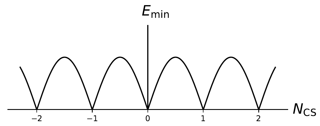
Figure 1: Sketch of the minimal field energy for a given value of the Chern-Simons number $N_{\rm CS}$. The energy approaches the minima with nonzero slope (Akiba, Kikuchi, and Yanagida, 1988).

The dissipation rate $\gamma$ can be related to the properties of thermal fluctuations of baryon number around its equilibrium value $B_{\rm eq}$: If $B-B_{\rm eq}$ has made a fluctuation to a nonzero value, this will tend to zero at the rate $\gamma$. Therefore, the time-dependent correlation function of the fluctuation reads

$$\langle[B(t)-B_{\rm eq}][B(0)-B_{\rm eq}]\rangle=\langle[B-B_{\rm eq}]^{2}\rangle e^{-\gamma|t|}\ ,$$ (10)

which implies

$$\langle[B(t)-B(0)]^{2}\rangle=2\langle[B-B_{\rm eq}]^{2}\rangle\left(1-e^{-\gamma|t|}\right).$$ (11)

For $t\ll\gamma^{-1}$ this grows approximately linearly with time:

$$\langle[B(t)-B(0)]^{2}\rangle\simeq 2\langle[B-B_{\rm eq}]^{2}\rangle\gamma|t|\ .$$ (12)

The mean square fluctuation on the right-hand side is determined by equilibrium thermodynamics and is proportional to the volume of the system $V$. It has to be evaluated at fixed $B-L$. The leading-order computation is straightforward but requires some care  Khlebnikov and Shaposhnikov (1996). In the temperature range between the electroweak transition and the equilibration temperature of the right-handed electron Yukawa interaction, it takes the value

$$\langle[B-B_{\rm eq}]^{2}\rangle=VT^{3}\frac{2n_{f}(5n_{f}+3N_{s})}{3(22n_{f}+13N_{s})}\ ,$$ (13)

where $N_{s}$ is the number of Higgs doublets. At lower temperatures one has to take into account a nonzero Higgs expectation value, and at higher temperatures there are additional conserved charges, which reduces the size of the fluctuation  Rubakov and Shaposhnikov (1996).

Owing to Eq. (3) the left-hand side of Eq. (12) is determined by the dynamics of the gauge fields:

$$\langle[B(t)-B(0)]^{2}\rangle=n_{f}^{2}\left\langle Q^{2}(t)\right\rangle\ .$$ (14)

For Eqs. (12) and (14) to be consistent, $Q$ in Eq. (7) must satisfy

$$\left\langle Q^{2}(t)\right\rangle=\Gamma_{\rm sph}V|t|.$$ (15)

This can be easily visualized with the help of Fig. 1. Most of the time the system sits near one of the minima, but every once in a while there is a thermal fluctuation that lets it hop to a neighboring one. This gives rise to a random walk leading to the behavior in Eq. (15). $\Gamma_{\rm sph}$, the number of transitions per unit time and unit volume, is known as the Chern-Simons diffusion rate or sphaleron rate. It can be estimated as

$$\Gamma_{\rm sph}\sim t_{\rm tr}^{-1}\ell^{-3},$$ (16)

where $t_{\rm tr}$ is the time of a single transition, and $\ell$ is the spatial size of the corresponding field configuration. The U(1) hypercharge gauge field does not contribute to the diffusive behavior in Eq. (15), so we neglect it here.

The linear growth with time can only be valid on timescales that are large compared to $t_{\rm tr}$. On the other hand, the linear growth can be valid only on timescales that are small compared to $\gamma^{-1}$. If there is a time window in which Eqs. (12) and (15) are both valid, which will be checked a posteriori, then one can match the two expressions to determine $\gamma$, which gives

$$\gamma=\frac{n_{f}^{2}\Gamma_{\rm sph}V}{2\langle[B-B_{\rm eq}]^{2}\rangle}\ .$$ (17)

Using $\langle[B-B_{\rm eq}]^{2}\rangle\sim VT^{3}$ one can therefore estimate $\gamma t_{\rm tr}\sim(\ell T)^{-3}$. Hence, the window exists if the size of the relevant field configurations is large compared to $T^{-1}$.

At low temperatures the $N_{\rm CS}$-changing transitions still proceed through tunneling. The probability for thermal transitions over the sphaleron barrier is proportional to $\exp(-E_{\rm sph}/T)$ (Kuzmin, Rubakov, and Shaposhnikov, 1985). They become dominant when $E_{\rm sph}/T\mbox{~{}{\raisebox{1.72218pt}{$<$}} {\raisebox{-2.58334pt}{$\sim$}}~{}}1/g^{2}$. The energy and the size of a sphaleron are of the order of $E_{\rm sph}\sim v/g$ and $\ell_{\rm sph}\sim 1/gv$, respectively. Therefore, the size of the sphaleron is larger than $T^{-1}$ when the thermal activation dominates, and the assumptions leading to Eq. (17) are valid in this case. For field configurations with $k\sim\ell^{-1}\mbox{~{}{\raisebox{1.72218pt}{$<$}} {\raisebox{-2.58334pt}{$\sim$}}~{}}T$, the occupation number, given by the Bose-Einstein distribution, is large [$f_{\rm B}(k)\simeq T/k\mbox{~{}{\raisebox{1.72218pt}{$>$}} {\raisebox{-2.58334pt}{$\sim$}}~{}}1$], so such fields can be treated classically.

The Higgs expectation value decreases with increasing temperature: see Fig. 2 and Sec. III.1. Therefore, the exponential suppression has already disappeared near the electroweak phase transition or crossover. The prefactor of the exponential corresponds to a one-loop computation of the fluctuations around the sphaleron contribution. The bosonic part was computed by (Arnold, Son, and Yaffe, 1997), and the fermionic contributions were obtained by Moore (1996).

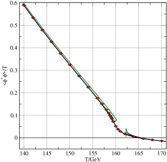
Figure 2: Temperature dependence of the expectation value of $\phi^{\dagger}\phi$ in the standard model. $\phi$ is the Higgs field. The points are the results of lattice simulations, and the full line is an interpolation of the data. The observable $\langle\phi^{\dagger}\phi\rangle$ can become negative, because it is ultraviolet divergent and additively renormalized. The shaded bands represent perturbative results for the broken and symmetric phases; their thickness estimates unknown higher-order contributions. From D’Onofrio and Rummukainen (2016).

In the symmetric phase the Higgs expectation value vanishes and there is no sphaleron solution. The length scale for $N_{\rm CS}$-changing field configurations can now be easily determined. When the energy of a field configuration is dominated by the electroweak magnetic field ${\bf B}={\bf D}\times{\bf A}$, it can be estimated as

$$E\sim\ell^{3}{\bf B}^{2}\sim\ell{\bf A}^{2}\ .$$ (18)

Using ${\bf E}\sim{\bf A}/t_{\rm tr}$, the change of Chern-Simons number is then given by

$$Q\sim g^{2}t_{\rm tr}\ell^{3}{\bf E}\cdot{\bf B}\sim g^{2}\ell^{2}{\bf A}^{2}\ .$$ (19)

If we require $Q\sim 1$ and $E\mbox{~{}{\raisebox{1.72218pt}{$<$}} {\raisebox{-2.58334pt}{$\sim$}}~{}}T$ to avoid Boltzmann suppression, we obtain $\ell\mbox{~{}{\raisebox{1.72218pt}{$>$}} {\raisebox{-2.58334pt}{$\sim$}}~{}}(g^{2}T)^{-1}$. But $(g^{2}T)^{-1}$ is the length scale beyond which static non-Abelian magnetic fields are screened. Time-dependent fields can be screened on even shorter length scales. Therefore, the relevant length scale for $N_{\rm CS}$-changing transitions in the symmetric phase is Arnold and McLerran (1987)

$$\ell\sim\frac{1}{g^{2}T}\ .$$ (20)

The corresponding gauge field is of the order of ${\bf A}\sim gT$. Therefore, both terms in the covariant derivative ${\bf D}-ig{\bf A}$ are of the same order of magnitude, and the second term cannot be treated as a perturbation. This leads to the breakdown of finite-temperature perturbation theory at this scale Linde (1980). Standard Euclidean (imaginary-time) lattice methods are not capable of computing real-time dynamics. However, since the relevant fields have large occupation numbers they can be approximated as classical fields, and $\Gamma_{\rm sph}$ can be computed by solving classical field equations of motion Ambjorn et al. (1991), where some care is needed to use the correct equations of motion.

The time evolution of the fields responsible for the sphaleron transitions is influenced by plasma effects (Arnold and McLerran, 1987; Arnold, Son, and Yaffe, 1997). The time-dependent gauge field has the nonvanishing electric field ${\bf E}$, which induces a current because the plasma is a good conductor. The relevant charges are the weak SU(2) gauge charges. The current is carried mostly by particles with hard momenta of the order of $T$ that are not described by classical fields. Therefore, the classical field equations are not appropriate for computing $\Gamma_{\rm sph}$. However, one can use effective classical equations of motion that should properly include the effect of the high-momentum particles. The mean free path of the particles is smaller than the length scale $\ell$. Therefore, the current can be written as $\sigma{\bf E}$ with the following conductivity of SU(2) charges $\sigma$:

$$\sigma=\frac{4\pi}{3}\frac{m^{2}_{\rm D}}{Ng^{2}T}\frac{1}{\log(1/g)}\sim\frac{T}{\log(1/g)}\ ,$$ (21)

where $N=2$ for SU(2) and $m_{\rm D}^{2}=(4N+2N_{s}+N_{F})g^{2}T^{2}/12$ is the Debye mass squared for $N_{F}$ chiral fermions and $N_{s}$ scalars in the fundamental representation. In the $A_{0}=0$ gauge ${\bf E}=-\dot{{\bf A}}$. Therefore, the current gives rise to a damping term in the equation of motion for ${\bf A}$. Estimating ${\bf D}\times{\bf B}\sim\sigma{\bf E}$ gives

$$t_{\rm tr}\sim\sigma\ell^{2}\sim[g^{4}\log(1/g)T]^{-1},$$ (22)

which is much larger than $\ell$. Thus, the gauge field is strongly damped and one can neglect $\dot{{\bf E}}$ in the equation of motion, which becomes Bodeker (1998)

$${\bf D}\times{\bf B}=\sigma{\bf E}+\bm{\zeta}\ .$$ (23)

$\bm{\zeta}$ is also part of the current of high-momentum particles. It is due to thermal fluctuations of all field modes with momenta larger than $g^{2}T$, and it is a Gaussian white noise that carries vector and group indices. It satisfies

$$\langle\zeta^{ia}(x)\zeta^{jb}(x^{\prime})\rangle=2T\sigma\delta^{ij}\delta^{ab}\delta(x-x^{\prime})\ ,$$ (24)

so that Eq. (23) is a Langevin equation. The estimate (16) then gives

$$\Gamma_{\rm sph}\sim g^{10}\log(1/g)T^{4}\ .$$ (25)

The numerical coefficient can be computed by solving Eq. (23) on a spatial lattice and determining $\Gamma_{\rm sph}$ from Eq. (15). The result can be written as

$$\Gamma_{\rm sph}=\kappa\frac{2\pi T}{3\sigma}\alpha^{5}T^{4},$$ (26)

with $\kappa=10.8\pm 0.7$ Moore (2000d) and $\sigma$ from Eq. (21). The mean free path of hard particles is short compared to $\ell$ by only a relative factor $\log(1/g)$. Nevertheless, Eq. (26) is still valid at next-to-leading logarithmic order if $\log(1/g)$ in Eq. (21) is replaced by $\log(m_{\rm D}/\gamma)+C$, where $\gamma=(Ng^{2}T/4\pi)\log(m_{\rm D}/\gamma)$ and $C\simeq 3.041$ Arnold and Yaffe (2000); Moore (2000c).

Close to the electroweak phase transition or crossover the thermal Higgs mass can become small, so that the Higgs field can affect the dynamics at the scale $g^{2}T$. The effective theory described by Eq. (23) has been extended to include the Higgs field  Moore (2000c). $\kappa$ also depends on the Higgs self-coupling and thus on the Higgs mass. In the standard model, just above the crossover temperature one finds that (D’Onofrio, Rummukainen, and Tranberg, 2014) $\Gamma_{\rm sph}/T^{4}=(8.0\pm 1.3)\times 10^{-7}\approx(18\pm 3)\alpha_{W}^{5}$. In the last form, factors of $\ln\alpha_{W}$ have been absorbed in the numerical constant. Without the Higgs field the rate is $\Gamma\approx(25\,\pm\,2)\,\alpha_{W}^{5}T^{4}$ (Moore, Hu, and Muller, 1998; Moore, 2000a).

Beyond logarithmic accuracy, the current is not simply a local conductivity times the electric field. To go beyond this approximation one has to solve the coupled equations for the gauge fields and the high-momentum particles. Here fields with ${\bf k}\sim gT$ are also important because they mediate the scattering of the high-momentum particles, which is small-angle scattering that changes the charge of the particles. For these modes one cannot neglect the term $\dot{{\bf E}}$, which leads to ultraviolet divergences in the simulation prohibiting a continuum limit (Bodeker, McLerran, and Smilga, 1995).

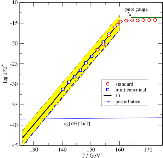
Figure 3: The Standard Model sphaleron rate computed on the lattice and the fit to the broken phase rate [Eq. (27], shown with a shaded error band. At low temperatures the sphaleron rate is exponentially small, which requires a special multicanonical method for the simulation. The perturbative result (Burnier, Laine, and Shaposhnikov, 2006) is the one-loop approximation to an expansion around the sphaleron solution. Pure gauge refers to the rate in hot SU(2) gauge theory. The sphalerons freeze out when $\Gamma$ crosses the appropriately scaled Hubble parameter, which is shown as the almost horizontal line. From D’Onofrio, Rummukainen, and Tranberg (2014).

When the Higgs expectation value is sufficiently large, the sphaleron rate becomes exponentially suppressed and one can perform a perturbative expansion around the sphaleron solution. The signal in lattice simulations, on the other hand, becomes small, which requires the use of a special multicanonical method Moore (1999). The current knowledge of the sphaleron rate in the standard model is summarized in Fig. 3. In the temperature range $130<T<159~{}\text{GeV}$ it can be parametrized as (D’Onofrio, Rummukainen, and Tranberg, 2014)

$$\log(\Gamma_{\rm sph}/T^{4})=(0.83\pm 0.01)\frac{T}{\rm GeV}-(147.7\pm 1.9),$$ (27)

which is the fit shown in Fig. 3. The rate computed on the lattice is larger than the perturbative results (Burnier, Laine, and Shaposhnikov, 2006) but consistent within errors. The corresponding values of the Higgs expectation value are depicted in Fig. 2.

At high temperatures, the sphaleron rate again becomes smaller than the Hubble parameter, which happens at $T\mbox{~{}{\raisebox{1.72218pt}{$>$}} {\raisebox{-2.58334pt}{$\sim$}}~{}}10^{12}$ GeV  Rubakov and Shaposhnikov (1996).

In theories with an extended Higgs sector, it is not obvious how to determine the freeze-out condition from the SM results, because the sphaleron solution can be different. In the symmetric phase this is somewhat easier. New particles interacting with the SU(2) gauge fields would increase the Debye mass $m_{\rm D}$ appearing in Eq. (21), thus decreasing the hot sphaleron rate. On the other hand, new particles would increase the Hubble parameter. Therefore the SM freeze-out temperature is an upper bound for the temperature below which $\gamma>H$.

In QCD with vanishing quark masses, the axial quark number is classically conserved, but it is also violated by the chiral anomaly. This process plays a role in both electroweak baryogenesis and leptogenesis. At finite temperature the Chern-Simons number of the gluon field can diffuse as in the electroweak theory in the symmetric phase, and the rate for anomalous axial quark number violation is again proportional to the Chern-Simons diffusion rate, which is then referred to as the strong-sphaleron rate. At high temperatures the quantum chromodynamics (QCD) coupling $\alpha_{\rm s}$ is weak, and the dynamics of the gluon fields is described by Eqs. (21)-(24) for SU(3) instead of SU(2). At the electroweak scale $\alpha_{\rm s}$ appears to be too large for the weak-coupling expansion to be valid. Using a different method, the strong-sphaleron rate at this scale was computed as $\Gamma_{\rm strong\>sph}\simeq 1.4\times 10^{-3}T^{4}$ Moore and Tassler (2011).

Strong sphalerons are most likely the only sphalerons that can be created in experiments. It has been argued that they could lead to observable signals in relativistic heavy ion collisions through the chiral magnetic effect Kharzeev (2014). In the simultaneous presence of a chiral imbalance and a magnetic field there is an electric vector current in the direction of the magnetic field. Such a current separates electric charges and could lead to measurable charge asymmetries. The required imbalance of left- and right-handed (anti)quarks can be caused by random strong-sphaleron transitions. Furthermore, if the collision of the heavy ions is not head-on, the remnants of the projectiles produce strong magnetic fields. There are ongoing experimental efforts to search for the chiral magnetic effect in heavy ion collisions. A dedicated run has been performed at the Brookhaven Relativistic Heavy Ion Collider colliding Ru on Ru and Zr on Zr (results are expected in 2021). These two nuclei are isobars, i.e., they have the same number of nucleons but different numbers of protons ($Z=44$ for Ru and $Z=40$ for Zr). Thus, the magnetic field is larger for Ru, so the charge asymmetries in Ru collisions should be larger than those in Zr (Wen, 2018; Kharzeev and Liao, 2021).

II.3 Baryon and lepton asymmetries

Quarks, leptons and Higgs bosons interact via Yukawa and gauge couplings and, in addition, via the nonperturbative sphaleron processes. In the temperature range $100<T<10^{12}\ \text{GeV}$, which is of interest for baryogenesis, gauge interactions, including the sphaleron interactions, are in equilibrium, i.e., their rate is larger than the Hubble parameter. On the other hand, Yukawa interactions are in equilibrium only in a more restricted temperature range that depends on the strength of the Yukawa couplings. Thus, in different temperature ranges there are different sets of charges that are conserved, which leads to the “flavor effects” that are discussed in Sec. IV.3.2. The corresponding partition function can be written as

$$Z(\mu,T,V)=\text{Tr}\exp\Big{\{}\beta\Big{(}\sum_{i}\mu_{i}Q_{i}-H\Big{)}\Big{\}}\ ,$$ (28)

where $\beta=1/T$ and $H$ is the Hamiltonian. For each of the quark, lepton, and Higgs fields, there is an associated chemical potential $\mu_{i}$; the corresponding charge operator is denoted by $Q_{i}$. In the standard model, with one Higgs doublet $\phi$ and $n_{f}$ families one has $5n_{f}+1$ chemical potentials $\mu_{i}$.

The processes that are in thermal equilibrium, the so-called spectator processes, yield constraints between the various chemical potentials Harvey and Turner (1990). The $N_{\rm CS}$-changing transitions (see Sec. II.2) change baryon and lepton numbers in each family by the same amount. They affect only the left-handed fermion fields, so that

$$\sum_{i}\left(3\mu_{qi}+\mu_{li}\right)=0\;.$$ (29)

One also has to take the SU(3) QCD sphaleron processes into account Mohapatra and Zhang (1992). They change the chiral quark number (the number of right-handed minus number of left-handed quarks) for each quark flavor by the same amount, so that

$$\sum_{i}\left(2\mu_{qi}-\mu_{ui}-\mu_{di}\right)=0\;.$$ (30)

The Yukawa interactions that are in equilibrium yield relations between the chemical potentials of the left-handed and right-handed fermions and the Higgs:

$$-\mu_{qi}+\mu_{dj}=\mu_{qi}-\mu_{uj}=-\mu_{li}+\mu_{ei}=\mu_{\phi}\ .$$ (31)

The remaining independent chemical potentials are subject to another condition, valid at all temperatures, that arises from the requirement that the total hypercharge of the plasma vanish.

In a weakly coupled plasma, the asymmetry between particle and antiparticle number densities is given by

$$n_{i}-n_{\bar{i}}=-\frac{\partial}{\partial\mu_{i}}\frac{T}{V}\ln{Z(\mu,T,V)}\ .$$ (32)

When computing the derivative in Eq. (32), all $\mu_{i}$ have to be treated as independent. For massless particles one obtains

$$n_{i}-n_{\bar{i}}={g_{i}T^{3}\over 6}\left\{\begin{array}[]{rl}\beta\mu_{i}+{\cal O}\big{(}\left(\beta\mu_{i}\right)^{3}\big{)}&(\text{fermions})\ ,\\ 2\beta\mu_{i}+{\cal O}\left(\big{(}\beta\mu_{i}\right)^{3}\big{)}&(\text{bosons})\ ,\end{array}\right.$$ (33)

where $g_{i}$ denotes the number of internal degrees of freedom. The following analysis is based on these relations for small chemical potentials ($\beta\mu_{i}\ll 1$).

Using Eq. (33) and the known hypercharges one can write the condition for hypercharge neutrality as

$$\sum_{i}\left(\mu_{qi}+2\mu_{ui}-\mu_{di}-\mu_{li}-\mu_{ei}\right)=2\mu_{\phi}\ ,$$ (34)

and the baryon-number and lepton-number densities can be expressed in terms of the chemical potentials as follows:

$$n_{B} =\frac{T^{2}}{6}\sum_{i}\left(2\mu_{qi}+\mu_{ui}+\mu_{di}\right)\;,$$ (35)

$$n_{L_{i}} =\frac{T^{2}}{6}(2\mu_{li}+\mu_{ei})\;.$$ (36)

Consider now the temperatures at which all Yukawa interactions are in equilibrium, which is the case for $T<85$ TeV Bodeker and Schröder (2019), but still above the electroweak transition. The quark chemical potentials are family independent, $\mu_{qi}=\mu_{q}$, $\mu_{ui}=\mu_{u}$, and $\mu_{di}=\mu_{d}$, and the asymmetries $L_{i}-B/n_{f}$ are conserved. For simplicity, we assume that they are all equal, so that the lepton chemical potentials are family-independent as well: $\mu_{li}=\mu_{l}$, $\mu_{ei}=\mu_{e}$. Using the sphaleron relation and the hypercharge constraint, one can express all chemical potentials, and therefore all asymmetries, in terms of a single chemical potential that may be chosen as $\mu_{l}$:

$$\frac{\mu_{e}}{\mu_{l}} ={2n_{f}+3\over 6n_{f}+3}\ ,\ \frac{\mu_{d}}{\mu_{l}}=-{6n_{f}+1\over 6n_{f}+3}\ ,\ \frac{\mu_{u}}{\mu_{l}}={2n_{f}-1\over 6n_{f}+3}\ ,$$

$$\frac{\mu_{q}}{\mu_{l}} =-{1\over 3}\ ,\ \frac{\mu_{\phi}}{\mu_{l}}=-{4n_{f}\over 6n_{f}+3}\ .$$ (37)

The corresponding baryon and lepton asymmetries are

$$n_{B}=-{4n_{f}\over 3}\frac{T^{2}}{6}\mu_{l}\;,\quad n_{L}={14n_{f}^{2}+9n_{f}\over 6n_{f}+3}\frac{T^{2}}{6}\mu_{l}\;.$$ (38)

Equation (38) yields the connection between the $B$, $B-L$, and $L$ asymmetries Khlebnikov and Shaposhnikov (1988)

$$B=c_{s}(B-L)\ ,\quad L=(c_{s}-1)(B-L)\ ,$$ (39)

where $c_{s}=(8n_{f}+4)/(22n_{f}+13)$. Near the electroweak transition the ratio $B/(B-L)$ is a function of $\langle\phi\rangle/T$ Laine and Shaposhnikov (2000).

The relations (39) between $B$, $B-L$, and $L$ numbers suggest that $B-L$ violation is needed in order to generate a baryon asymmetry at high temperatures where sphaleron processes are in thermal equilibrium. Because the $B-L$ current has no anomaly, the value of $B-L$ at time $t_{f}$, where the leptogenesis process is completed, determines the value of the baryon asymmetry today:

$$B(t_{0})=c_{s}(B-L)(t_{f})\;.$$ (40)

On the other hand, during the leptogenesis process the strength of ($B-L$)-violating, and therefore $L$-violating interactions can only be weak. Otherwise, because of Eq. (39), they would wash out any baryon asymmetry. As we later see, the interplay between these conflicting conditions leads to important constraints on the properties of the neutrinos.

The situation is different for electroweak baryogenesis. Here $B-L=0$ and the change of the sphaleron rate across the bubble wall in a first-order phase transition is essential for the generation of a baryon asymmetry.

III Electroweak baryogenesis

Electroweak baryogenesis is a sophisticated nonequilibrium process at the electroweak phase transition (Cohen, Kaplan, and Nelson, 1993). We first describe the nature of the phase transition and the basic idea of the charge transport mechanism. We then illustrate the status of electroweak baryogenesis by some representative examples, corresponding to a weakly as well as a strongly interacting Higgs sector. Special emphasis is placed on the implications of recent stringent upper bounds on the electron electric dipole moment.

III.1 Electroweak phase transition

Electroweak baryogenesis requires a first-order phase transition to satisfy the Sakharov condition of nonequilibrium. It has to be strongly first order, meaning that in the low-temperature phase the sphaleron rate is sufficiently suppressed and the just created asymmetry is not washed out; see Sec. III.2.

At zero temperature the electroweak symmetry is broken by the vacuum expectation value of the Higgs field $\phi$, giving mass to the electroweak gauge bosons and to fermions. At high temperature the Higgs expectation value vanishes. The symmetry that is broken by the expectation value is a gauge symmetry, not a symmetry transforming physical states. Therefore, it is not guaranteed that there will be a phase transition associated with the change of $\langle\phi\rangle$. (Nevertheless, it is common nomenclature to speak about a symmetry-broken and a symmetric phase.)

The expectation value of $\phi$ is obtained by minimizing the effective potential $V_{\rm eff}$, which can be defined as $V_{\rm eff}(\phi)\equiv-P(\phi)$, where $P(\phi)$ is the pressure in the presence of a constant classical value $\phi$ of the Higgs field. It includes the tree-level Higgs potential $V_{\text{tree}}$. To first approximation it is given by the difference of $V_{\text{tree}}$ and the pressure of an ideal gas $P_{\rm ideal}$. When the temperature is much larger than the particle mass $M$, the pressure of an ideal gas is, according to standard thermodynamics,

$$P_{\rm ideal}=T^{4}\left(a-b\frac{M^{2}}{T^{2}}+c\frac{M^{3}}{T^{3}}+O\left(M^{4}/T^{4}\right)\right)\ ,$$ (41)

with positive constants $a$ and $b$. The $O(M^{2}/T^{2})$ contribution is negative because a nonzero mass reduces the momentum of a particle with a given energy and thus the pressure. If the particle masses are proportional to the value of the Higgs field, then a smaller $\phi$ leads to larger pressure. A phase with a smaller $\phi$ will push out one with a larger value of the Higgs, so that the Higgs expectation value becomes zero. Therefore, at high temperature the electroweak symmetry is unbroken. The region where this happens can be expected to be of the order of the weak gauge-boson mass.

Beyond the ideal gas approximation one can compute the effective potential as follows. One integrates out all field modes with nonzero momentum in the imaginary-time path integral:

$$e^{-\beta VV_{\rm eff}(\phi)}=\int^{\prime}{\cal D}\Phi\exp\left\{-S_{E}[\Phi]\right\}\ ,$$ (42)

with the Euclidean, or imaginary-time, action ($t=-i\tau$)

$$S_{E}=-\int_{0}^{\beta}d\tau\int d^{3}x{\cal L}\ .$$ (43)

$\Phi$ denotes the set of all fields of our system, and the prime indicates that the integration over the zero-momentum modes $\phi$ is omitted. The partition function $Z=\exp(\beta VP)$ is then obtained by integrating Eq. (42) over $\phi$. This is done in the saddle-point approximation, which gives the minimum condition for $V_{\rm eff}(\phi)$. In the one-loop approximation Eq. (42) gives $-V_{\rm eff}$ as the difference between $P_{\rm ideal}$ and the $T=0$ contribution to the effective potential Coleman and Weinberg (1973).

For illustration, first consider the case of a single real scalar field $\varphi$ with the Lagrangian

$${\cal L}=\tfrac{1}{2}\partial_{\mu}\varphi\partial^{\mu}\varphi-V_{\text{tree}}(\varphi)$$ (44)

and the potential

$$V_{\text{tree}}(\varphi)=\frac{\mu^{2}}{2}\varphi^{2}+\frac{\lambda}{4}\varphi^{4}\ ,$$ (45)

with $\mu^{2}<0$, so that the minima of the potential are at $\varphi=\pm v=\pm\sqrt{-\mu^{2}/\lambda}$, spontaneously breaking the symmetry $\varphi\to-\varphi$. Now the mass of a particle in the constant “background” field $\varphi$ is $M^{2}(\varphi)=V^{\prime\prime}_{\rm tree}(\varphi)=\mu^{2}+3\lambda\varphi^{2}$. Equation (41) then gives

$$V_{\rm eff}(\varphi)=\frac{1}{2}\left(\mu^{2}+\frac{\lambda}{4}T^{2}\right)\varphi^{2}+\frac{\lambda}{4}\varphi^{4}+O(M^{3}/T)\ ,$$ (46)

where we have omitted the $\varphi$-independent terms. At finite temperature there is a positive contribution $\lambda T^{2}/4$ to the coefficient of the quadratic term, the so-called thermal mass (squared). It drives the expectation value to smaller values. When $T\gg 2\sqrt{-\mu^{2}/\lambda}$, the expectation value vanishes and the symmetry is restored.

Figure 4: Effective potential giving rise to a first-order phase transition. The value at $\varphi=0$ is subtracted.

One may worry that at small $\varphi$, with decreasing temperature $M^{2}(\varphi)$ becomes zero and eventually negative, so that the $O(M^{3}/T)$ term in Eq. (46) would give an imaginary part to the effective potential. However, it turns out that the loop-expansion parameter is $\lambda T/M$ Arnold and Espinosa (1993). Therefore, perturbation theory breaks down when $M$ becomes too small and is thus not reliable for determining the details of the phase transition. It is, in fact, second order, and the value of $\varphi$ changes continuously from zero above the critical temperature $T_{c}$ to a nonzero value below $T_{c}$.

Next consider the SM with one Higgs doublet $\phi$. The tree-level potential is written as in Eq. (45) with $\varphi=\sqrt{2\phi^{\dagger}\phi}$. Now all SM species contribute to the pressure and thus to $V_{\rm eff}$. There is a qualitatively new effect compared to the previous example. Since the electroweak gauge bosons obtain their mass from the Higgs field and have no tree-level mass term, they contribute with $M^{2}\sim g^{2}\phi^{\dagger}\phi$ in Eq. (41). The $M^{3}/T$ term in Eq. (41) then gives rise to a cubic term in the effective potential

$$V_{\rm eff}(\varphi)=\frac{A}{2}\left(T^{2}-T^{2}_{b}\right)\varphi^{2}-\frac{B}{3}\varphi^{3}+\frac{\lambda}{4}\varphi^{4}+\cdots.$$ (47)

This potential would give a first-order phase transition, as illustrated in Fig. 4. At the critical temperature $T_{c}$ there are two degenerate minima. $T_{b}\equiv\sqrt{-\mu^{2}/A}$ is the temperature below which the potential barrier vanishes and the local minimum at $\varphi=0$ disappears.

In the SM $B$ is small. Therefore, the symmetry breaking minimum $\varphi_{c}$ is small, and so is the effective gauge-boson mass $M$. The loop-expansion parameter $g^{2}T/M$ is again large, so perturbation theory cannot be trusted. Using nonperturbative methods it was shown that for Higgs masses larger than about 70-80 GeV, and thus in the SM, there is no electroweak phase transition but a smooth crossover Buchmuller and Philipsen (1995); Kajantie et al. (1996); Csikor et al. (1999). The Higgs expectation value changes continuously with temperature, as shown in Fig. 2. Hence, during the transition the system stays close to thermal equilibrium and Sakharov’s third condition is not satisfied.

A strongly first-order phase transition is possible only in extensions of the SM. Since large field values imply large $M^{2}(\varphi)$, the effective potential can be computed perturbatively. However, one may not be able to use the previously descrribed high-temperature expansion, in which case even the one-loop effective potential cannot be written in a simple analytic form. A comprehensive discussion of the theoretical uncertainties was recently given by Croon et al. (2020).

Since the high-temperature phase is metastable as long as there is a potential barrier separating the two minima, the Universe supercools to some $T<T_{c}$; see  Fig. 4. Bubbles of the symmetry-broken phase form through thermal fluctuations with a probability that can be computed using a saddle-point approximation in statistical mechanics Langer (1969). The probabilty of forming a bubble per time and volume is $A\exp(-\beta S_{\rm eff}[\phi_{\rm bubble}])$, where the effective potential $V_{\rm eff}(\phi)$ [see Eq. (42)] has been replaced by the effective action $S_{\rm eff}$ at the bubble configuration $\phi_{\rm bubble}$ Linde (1981). It is the free energy of a static configuration representing a barrier between the metastable state and a state with a bubble of the low-temperature phase, similar to the sphaleron barrier; cf. Sec. II.2. The temperature-dependent prefactor $A$ is due to fluctuations around the saddle point and can be computed perturbatively Morrissey and Ramsey-Musolf (2012). Nonperturbative lattice computations of the nucleation rate indicate that perturbation theory slightly underestimates the strength of the phase transition while overestimating the amount of supercooling Moore and Rummukainen (2001).

The bubbles nucleate roughly when the nucleation rate equals $H^{4}$, i.e., when one bubble nucleates per Hubble volume and time. Since around the electroweak scale $H\sim T_{c}^{2}/M_{\rm Pl}\sim 10^{-17}T_{c}$, the rate is extremely small. Once formed, the bubbles expand and begin to fill the entire Universe with the low-temperature phase. Important parameters of this process are the velocity $v_{\rm w}$ of the wall separating the two phases and their thickness $\ell_{\rm w}$ in the wall frame. The bubble wall velocity is determined by the pressure difference between the two phases. The pressure consists of the vacuum contribution, i.e. $-V_{\text{eff}}|_{T=0}$, and the pressure due to the plasma. When a particle mass depends on the value of the Higgs field it changes while the particle passes the wall. Therefore, there is a momentum transfer to the wall giving a contribution to the pressure. This includes a large contribution due to the magnetic-scale gauge fields (see Sec. II.2), which are suppressed in the symmetry-broken phase and get pushed out by the wall Moore (2000b). At the critical temperature the pressure difference between the two phases vanishes. The system is static and in thermal equilibrium. Below $T_{c}$, the wall moves into the high-temperature phase, the time dependence prevents the particle distribution from equilibration, and one has to deal with a nonequilibrium problem. One has to solve a set of Boltzmann equations which turns out to be difficult. The wall velocity is quite model dependent: it can vary from $v_{\rm w}\ll 1$ to $v_{\rm w}\sim 1$ in the plasma rest frame. For the SM it was found that $v_{\rm w}\sim 0.4$, and $\ell_{\rm w}T\sim 25$ Moore and Prokopec (1995), while in the minimal supersymmetric standard model (MSSM) $v_{\rm w}\mbox{~{}{\raisebox{1.72218pt}{$<$}} {\raisebox{-2.58334pt}{$\sim$}}~{}}0.1$ John and Schmidt (2001). Often the wall velocity is treated as a free parameter. A relatively simple case is ultrarelativistic bubbles with $\gamma_{\rm w}\equiv(1-v_{\rm w}^{2})^{-1/2}\gg 1$ Bodeker and Moore (2009). The reason is that the wall passes so fast that particles start scattering only when the wall has already passed. There are models in which, based on this analysis, the bubble wall can speed up indefinitely. However, additional radiation off the particles passing the wall leads to a speed limit Bodeker and Moore (2017); Höche et al. (2021).

III.2 Charge transport mechanism

When a phase-transition bubble wall sweeps through the plasma, it affects the motion of the particles therein. The dominant effect is spin independent and contributes to the pressure on the wall, as discussed in Sec. III.1. Subleading but essential for baryogenesis is the $CP$-violating separation of particles with different spins. On one side of the bubble wall there are more left-handed (negative helicity) particles and their negative helicity antiparticles than on the other side. In the symmetric phase electroweak sphalerons are unsuppressed. They act on left-handed particles and on right-handed antiparticles, and thus wash out the baryon number $B_{L}$ carried by the left-chiral fields describing left-handed particles and right-handed antiparticles. If the weak-sphaleron rate is sufficiently suppressed on the other side of the wall, a net baryon number is generated; for a comprehensive review of charge transport, see Konstandin (2013).

One distinguishes the thin-wall limit $\ell_{\rm w}\sim T^{-1}$ from the thick-wall limit $\ell_{\rm w}\gg T^{-1}$; i.e., the de Broglie wavelength of a typical particle $T^{-1}$ is small or of similar size relative to the wall thickness. In the former case, the particle-wall interaction is described by quantum reflection and transmission (Joyce, Prokopec, and Turok, 1996a).

In the thick-wall case the effect on the particles can be described as a semiclassical force (Joyce, Prokopec, and Turok, 1996b) that depends on their spin (Cline, Joyce, and Kainulainen, 2000). Interactions with the bubble wall give rise to space- and time-dependent mass terms, which may contain a $CP$-violating phase. For concreteness consider a single fermion field $\psi$ with

$${\cal L}_{\rm mass}=-\overline{\psi_{L}}m\psi_{R}-\overline{\psi_{R}}m^{\ast}\psi_{L}\ ,$$ (48)

where $m=|m|\exp(i\theta)$. Such a term can be due to interactions with varying scalar fields like in Eq. (57) in combination with the Yukawa interaction, or due to varying Yukawa couplings (Bruggisser, Konstandin, and Servant, 2017). Bubble walls quickly grow to macroscopic sizes and thus can be approximated as planar. Let the wall move in the $z$ direction. It is convenient to Lorentz boost to the rest frame on the bubble so that $m$ depends only on $z$. One can expand in derivatives of $m$, corresponding to an expansion in $(\ell_{\rm w}T)^{-1}$. Keeping the first two terms, one obtains the semiclassical force

$$F_{z}=-\frac{\left(|m|^{2}\right)^{\prime}}{2E}+s\left[\frac{\left(|m|^{2}\theta^{\prime}\right)^{\prime}}{2EE_{z}}-\frac{|m|^{2}\left(|m|^{2}\right)^{\prime}\theta^{\prime}}{4E^{3}E_{z}}\right]\ ,$$ (49)

with $E=({\bf p}^{2}+|m|^{2})^{1/2}$, $E_{z}=(p_{z}^{2}+|m|^{2})^{1/2}$, and $s=\pm 1$ for spin (as defined in the frame where the momentum transverse to the wall vanishes) in the $\pm z$ direction. The prime denotes derivatives with respect to $z$. The leading-order term is independent of spin. Because of the chiral nature of the mass term in Eq. (48) there is a spin dependence, which first appears at second order in Eq. (49). Note that Eq. (49) holds for all four states of the fermion.

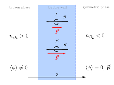
Figure 5: Sketch of the bubble wall (between the dashed lines) in the rest frame of the wall. More particles are crossing the wall from right to left. The force on tops with spin in the $+z$ direction is smaller than the force on antitops with spin in the $-z$ direction.

The forces on different (anti)particles are sketched in Fig. 5 with top quarks as an example, and with the square bracket in Eq. (49) assumed to be negative. For all (anti)tops the force is positive and pushes them toward the symmetric phase. The spin-dependent term is negative for left-handed (anti)tops and decreases the force acting on them, while it increases the force on right-handed (anti)tops. The left-handed tops carry positive $B_{L}$, while the right-handed antitops carry negative $B_{L}$. Therefore, the force changes the distribution of $B_{L}$ in space so that $n_{B_{L}}$ becomes nonzero and $z$ dependent.

The baryogenesis process is affected not only by the force but also by scattering and the wall velocity. In Fig. 5 it is assumed that these effects lead to $n_{B_{L}}<0$ in the symmetric phase. Without electroweak sphalerons the total asymmetry vanishes: $n_{B}=n_{B_{L}}+n_{B_{R}}=0$. In the symmetric phase electroweak sphalerons are unsuppressed and diminish $|n_{B_{L}}|$ leading to $n_{B}>0$. Since electroweak sphalerons are not active in the broken phase, this baryon asymmetry is frozen in after the phase transition is completed.

For a quantitative description the force is inserted into a Boltzmann equation, together with the collision terms describing particle scattering. For vanishing wall velocity the plasma is in local thermal equilibrium. Thus, for small wall velocity one can make a fluid ansatz, writing the phase-space densities as local equilibrium distributions with slowly varying chemical potentials, plus small perturbations $\delta f_{i}$, representing deviations from kinetic equilibrium (Joyce, Prokopec, and Turok, 1996b). One then takes moments of the Boltzmann equations, i.e., integrates over momentum with weights $1$ and $p_{z}/E$. The integrals of $(p_{z}/E)\delta f_{i}$ represent corrections $\delta v_{i}$ to the local fluid velocity. One obtains a network of coupled differential equations for $\delta v_{i}$ and $\mu_{i}$. One must also include the effect of the weak and strong sphalerons. The slowest interaction involves the weak-sphaleron transitions. Therefore, the equations for the chemical potentials can be computed by assuming baryon-number conservation, and finally the baryon asymmetry is computed from them. The resulting asymmetry is directly proportional to the weak-sphaleron rate in the symmetric phase. While most works have assumed small wall velocity and expanded in $v_{\rm w}$, baryogenesis with large $v_{\rm w}\sim 1$ was recently studied Cline and Kainulainen (2020). It was found, contrary to common lore, that baryogenesis with $v_{\rm w}$ larger than the speed of sound is possible, and that the generated asymmetry smoothly decreases with increasing $v_{\rm w}$.

During the entire process $B\!-\!L$ is unchanged because it is conserved by the sphaleron processes. Therefore the produced lepton asymmetry is of the same order of magnitude as the baryon asymmetry. If a larger lepton asymmetry would be observed, this would rule out electroweak baryogenesis as the sole origin of the baryon asymmetry of the Universe.

III.3 Perturbative models

In the SM the electroweak transition is only a smooth crossover but simple extensions allow for a strongly first-order phase transition. The first example to try is the two-Higgs-doublet model (2HDM), which has been extensively studied in the literature: for a review and references, see Branco et al. (2012b). Dorsch et al. (2017) thoroughly studied models of type II where leptons and down-type quarks couple to the Higgs doublet $\Phi_{1}$ while up-type quarks couple to the second Higgs doublet $\Phi_{2}$. The corresponding $\mathbb{Z}_{2}$ symmetry is softly broken by a complex mass term $\mu^{2}$, and the scalar potential reads

$$\begin{split}V_{\rm tree}=-&\mu^{2}_{1}\Phi_{1}^{\dagger}\Phi_{1}-\mu^{2}_{2}\Phi_{2}^{\dagger}\Phi_{2}-\frac{1}{2}\big{(}\mu^{2}\Phi_{1}^{\dagger}\Phi_{2}+{\rm H.c.}\big{)}\\ +&\frac{\lambda_{1}}{2}\big{(}\Phi_{1}^{\dagger}\Phi_{1}\big{)}^{2}+\frac{\lambda_{2}}{2}\big{(}\Phi_{2}^{\dagger}\Phi_{2}\big{)}^{2}\\ +&\lambda_{3}\big{(}\Phi_{1}^{\dagger}\Phi_{1}\big{)}\big{(}\Phi_{2}^{\dagger}\Phi_{2}\big{)}+\lambda_{4}\big{(}\Phi_{1}^{\dagger}\Phi_{2}\big{)}\big{(}\Phi_{2}^{\dagger}\Phi_{1}\big{)}\\ +&\frac{1}{2}\big{[}\lambda_{5}\big{(}\Phi_{1}^{\dagger}\Phi_{2}\big{)}^{2}+{\rm h.c.}\big{]}.\end{split}$$ (50)

In addition to $\mu^{2}$ the quartic coupling $\lambda_{5}$ can be complex, which leads to the complex vacuum expectation values

$$\langle\Phi_{1}\rangle=\frac{1}{\sqrt{2}}\begin{pmatrix}0\\ \,v\cos\beta\,\end{pmatrix},\ \langle\Phi_{2}\rangle=\frac{1}{\sqrt{2}}\begin{pmatrix}0\\ \,v\sin\beta\,e^{i\theta}\end{pmatrix}.$$ (51)

In addition to the observed Higgs boson $h^{0}$, the model contains four heavy Higgs bosons $H^{0}$, $A^{0}$ and $H^{\pm}$. There are two field-redefinition-invariant phases that can be written as

$$\delta_{1}={\rm arg}[(\mu^{2})^{2}\lambda_{5}^{*}]\ ,\quad\delta_{2}={\rm arg}(v_{1}v_{2}^{*}\,\mu^{2}\lambda_{5}^{*})\ .$$ (52)

A benchmark scenario has been studied with $m_{H_{0}}=200~{}\text{GeV}$ and $m_{A_{0}}=m_{H^{\pm}}$ at around $470~{}\text{GeV}$. At the cost of some tuning the masses can be increased by about $100~{}\text{GeV}$. The quartic couplings are large [$|\lambda_{i}|=\mathcal{O}(1)$] but satisfy the perturbativity bound $|\lambda_{i}|\lesssim 2\pi$ and tree-level unitarity, as well as constraints from flavor observables and the LHC. For these parameters, the phase transition is strongly first order ($v_{n}/T_{n}\geq 1$), where $v_{n}$ is the jump of the Higgs expectation value at the bubble nucleation temperature $T_{n}$. An interesting aspect of the model is that, due to the large quartic scalar couplings, a gravitational wave (GW) signal is predicted that would be observable at LISA.

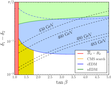
Figure 6: EDM constraints for parameter benchmarks corresponding to different heavy-Higgs-boson masses in the type-II 2HDM. The dash-dotted line shows the electron EDM (eEDM) bound before the ACME experiment. The black dashed lines indicate the minimum $CP$-violating phase necessary for successful baryogenesis, with $m_{H^{0}}=200~{}\text{GeV}$ and varying $m_{A^{0}}=m_{H^{\pm}}$. The green area is excluded by neutron EDM (nEDM) bounds, and the blue area is excluded by the electron EDM bound from ACME (2014). From Dorsch et al. (2017).

An attractive feature of electroweak baryogenesis models is also the connection between the $CP$ violation needed for baryogenesis and low-energy precision measurements. Particularly stringent are the following upper bounds on the electron dipole moment (EDM) obtained by the ACME eperiment Baron et al. (2014); Andreev et al. (2018):

$$\begin{split}\text{ACME~{}(2014)}:\quad|d_{e}|&<8.7\times 10^{-29}\ e\ {\rm cm}\ ,\\ \text{ACME~{}(2018)}:\quad|d_{e}|&<1.1\times 10^{-29}\ e\ {\rm cm}\ .\end{split}$$ (53)

The ACME bound from 2014 is indicated in Fig. 6 by the blue line, the lower boundary of the blue region. It is consistent with all theoretical and phenomenological constraints on the described model. The uncolored region represents the allowed parameter region at that time. The ACME bound from 2018 improves this upper bound by a factor of $8.7$. This excludes the parameter space of the model entirely.

For many years electroweak baryogenesis has also been studied in supersymmetric 2HDM models (MSSM). In this case the quartic scalar couplings are determined by gauge couplings. These models are now excluded due to the lower bounds on superparticle masses obtained at the LHC. These bounds and further theoretical constraints were described in detail by Cline (2018), together with a discussion of some nonsupersymmetric extensions of the standard model.

As an alternative to 2HDM models one can also consider a Higgs sector with one SU(2)-doublet Higgs $\Phi$ and an additional light SM singlet $s$, which is partially motivated by composite Higgs models. Electroweak baryogenesis for such a setup was studied by Espinosa et al. (2012); see also Cline and Kainulainen (2013), Bian, Wu, and Xie (2019), and Carena, Liu, and Wang (2019a). The renormalizable part of the effective scalar potential reads

$$V_{\text{tree}}=V^{\textrm{even}}+V^{\textrm{odd}}\ ,$$ (54)

with

$$\begin{split}V^{\text{even}}=&-\mu_{h}^{2}|\Phi|^{2}+\lambda_{h}|\Phi|^{4}\\ &-\frac{1}{2}\mu_{s}^{2}s^{2}+\frac{1}{4}\lambda_{s}s^{4}+\frac{1}{2}\lambda_{m}s^{2}|\Phi|^{2},\\ V^{\text{odd}}=&\frac{1}{2}\mu_{m}s|\Phi|^{2}+\mu_{1}^{3}s+\frac{1}{3}\mu_{3}s^{3}\ .\end{split}$$ (55)

The SU(2) doublet $\Phi$ contains the physical Higgs scalar $h$. The potential $V^{\text{even}}$ is invariant with respect to the $\mathbb{Z}_{2}$ symmetry

$$s\rightarrow-s\ ,$$ (56)

which is softly broken by the potential $V^{\text{odd}}$. The vacuum expectation value of $H$ implies mass mixing between $s$ and $h$.

Figure 7: Large contribution to the electron EDM from top loop and singlet-doublet mixing. From Espinosa et al. (2012).

An appropriate choice of quartic couplings and mass parameters $\mu_{i}\sim 100~{}\text{GeV}$ lead to a strongly first-order phase transition accompanied by baryogenesis. The required CP violation is provided by a dimension-5 operator (see Fig. 7)

$$\mathcal{L}_{tHs}=\frac{s}{f}\Phi\bar{q}_{L3}(a+ib\gamma_{5})t_{R}+\text{h.c.}\ ,$$ (57)

which couples the top quark to the scalars $\Phi$ and $s$. During the phase transition both scalars aquire an expectation value and the profile of $s$ provides the $CP$-violating top-quark scatterings. The compositeness scale has to be low ($f/b\sim 1~{}\text{TeV}$) so that strongly interacting resonances can be expected in the LHC range. For the light singlet $s$, a mass is predited to be comparable to the Higgs mass.

The mass mixing between $h$ and $s$ also generates an electron EDM; see Fig. 7. The analysis of Espinosa et al. (2012) was carried out while assuming the upper bound Hudson et al. (2011)

$$d_{e}<1.05\times 10^{-27}\ e\ \text{cm}\ .$$ (58)

The improvement of this bound by 2 orders of magnitude by the ACME experiment [Eq. (53)] excludes the model in its original form. A possible way out is to tune the parameters of the model such that a two-step phase transition occurs, with $s\neq 0$ during baryogenesis and $s=0$ in the zero-temperature vacuum Kurup and Perelstein (2017). At zero temperature the $\mathbb{Z}_{2}$ symmetry is then unbroken and the contribution to the electron EDM vanishes. Choosing $m_{s}>m_{h}/2$, the Higgs-boson decay width is unchanged and one obtains a “nightmare scenario” that is difficult to test at the LHC (Curtin, Meade, and Yu, 2014). For EWBG a new source of $CP$ violation is needed, for instance, $CP$ violation in a dark sector, which is transferred to the visible sector via a new light vector boson (Carena, Quirós, and Zhang, 2019b). However, such a construction eliminates one of the main motivations for electroweak baryogenesis: the connection between $CP$ violation measurable at low energies and the matter-antimatter asymmetry.

Figure 8: Electron EDM vs the lightest chargino mass in the split NMSSM for two parameter sets (setup 1, red dots; setup 2, green dots). The dotted line denotes the ACME (2014) upper bound $|d_{e}|<8.7\times 10^{-29}\ e\ \text{cm}$. We have added the dashed line that indicates the ACME (2018) upper bound $|d_{e}|<1.1\times 10^{-29}\ e\ \text{cm}$. Adapted from Demidov, Gorbunov, and Kirpichnikov (2016).

One may wonder whether EWBG can be more easily realized in models with more scalar fields. An example is the split next-to-minimal supersymmetric standard model (sNMSSM) (Demidov, Gorbunov, and Kirpichnikov, 2016), which contains two Higgs doublets $H_{u}$ and $H_{d}$ and an additional singlet $N$. The corresponding superpotential reads

$$W=\lambda NH_{u}H_{d}+\tfrac{1}{3}kN^{3}+\mu H_{u}H_{d}+rN\ .$$ (59)

Scalar quarks and leptons are removed from the low-energy spectrum but gauginos have electroweak-scale masses. The dominant role in EWBG is played by the scattering of charginos. At one-loop order they also lead to an EDM for the electron. According to the analysis of Demidov, Gorbunov, and Kirpichnikov (2016), a strongly first-order phase transition and EWBG are compatible with the ACME (2014) bound on the electron EDM. Figure 8 shows the electron EDM as a function of the lightest chargino mass for two parameter benchmarks. However, as the figure demonstrates, the stronger ACME (2018) bound again excludes this model.

The connection between EWBG and electron EDM has also been analyzed in a setup with the same particle content as the sNMSSM but without the relations between the Yukawa couplings implied by supersymmetry (Fuyuto, Hisano, and Senaha, 2016). As in the singlet-doublet model, a strongly first-order phase transition is possible, and EWBG is driven by Higgsino and singlino scatterings with masses $m_{\tilde{H}}$ and $m_{\tilde{S}}$, respectively. At two-loop order an electron EDM is generated which depends on the Higgsino masses.

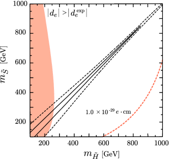
Figure 9: Contours of $\eta_{B}/\eta_{B}^{\text{observed}}=$ 1 (solid lines) and 0.1 (dashed lines) along the $(m_{\tilde{H}},m_{\tilde{S}})$ plane. The orange area is excluded by the ACME (2014) bound. The orange dashed line corresponds to the anticipated sensitivity $|d_{e}|=1.0\times 10^{-29}\ e\ \text{cm}$, which essentially agrees with the ACME (2018) bound. From Fuyuto, Hisano, and Senaha (2016).

In Fig. 9 a region of successful EWBG is shown along the $(m_{\tilde{H}},m_{\tilde{S}})$ plane for representative Higgsino couplings. The orange area on the left is excluded by the ACME (2014) bound, leaving a large range of viable Higgsino and singlino masses. However, the ACME (2018) bound again excludes this region. The electron EDM receives contributions from two graphs that have charged and neutral gauge bosons in the loop, respectively. Fine-tuning couplings, the contributions can cancel each other out, which would eliminate the connection between low-energy $CP$ violation and EWBG.

The upper bound on the electron EDM placed by the ACME experiment is an impressive achievement. The experiment uses a heavy polar molecule, thorium monoxide (ThO). In an external electric field it possesses states whose energies are particularly sensitive to the electron EDM. Moreover, the magnetic moment of these states is small, which makes the experiment relatively impervious to stray magnetic fields. A cryogenic beam source provides a high flux of ThO molecules. In 2014 these techniques led to an upper bound on the electron EDM more than 1 order of magnitude smaller than the best previous measurements Baron et al. (2014). Four years later the upper limit could be further improved by a factor of $8.7$ Andreev et al. (2018).

Studies of electroweak baryogenesis with two Higgs doublets began in the early 1990s Turok and Zadrozny (1991); McLerran et al. (1991), followed by other models with an extended Higgs sector. Over the years the increasing lower bound on the Higgs mass, and finally the discovery of a $125~{}\text{GeV}$ Higgs boson, as well as bounds on the heavier Higgs-boson masses from flavor observables and the LHC strongly constrained these models. Much progress was made in understanding the challenging dynamics of electroweak baryogenesis, and the possible connection to gravitational waves in the LISA frequency range was explored. In a complementary way, upper bounds on dipole moments played an increasingly important role since generic models of electroweak baryogenesis connect low-energy $CP$ violation with the baryon asymmetry of the Universe. As previously described, it appears that finally these bounds have become so strong that they essentially exclude all models of electroweak baryogenesis that can be treated perturbatively. These developments over 30 years represent an example of how the interplay of theory and experiment can guide us in our search for physics beyond the standard model.

III.4 Strongly interacting models

Thus far we have considered EWBG in perturbatively defined renormalizable extensions of the SM. However, it is also possible that the observed Higgs boson is a light state in a strongly interacting sector of dynamical electroweak symmetry breaking. This would qualitatively change the electroweak phase transition as well as EWBG, which can be treated by means of an effective field theory (Grojean, Servant, and Wells, 2005). The light Higgs boson could emerge from the spontaneous breaking of a global symmetry, such as SO(5) $\rightarrow$ SO(4), together with a dilaton as pseudo-Nambu-Goldstone boson from broken conformal symmetry in a strongly coupled hypercolor theory with partial compositeness; for a review, see Panico and Wulzer (2016). In such a framework EWBG was studied by Bruggisser et al. (2018a, b) based on an effective Lagrangian with a minimal set of couplings and masses Giudice et al. (2007); Chala et al. (2017). The analysis is based on the following effective potential for the Higgs $h$ and the dilaton $\chi$:

$$\begin{split}V_{\text{eff}}[h,\chi]&=\left(\frac{g_{\chi}}{g_{\star}}\chi\right)^{4}\left[\alpha\sin^{2}\left(\frac{h}{f}\right)+\beta\sin^{4}\left(\frac{h}{f}\right)\right]\\ &\quad+V_{\chi}(\chi)+\Delta V_{T}(h,\chi)\ ,\end{split}$$ (60)

where

$$\begin{split}\alpha[y]&=c_{\alpha}\sum_{i=1}^{N_{f}}\ g_{\star}^{2}{N_{c}y_{i}^{2}[\chi]\over(4\pi)^{2}}\ ,\ y_{i}[\chi]\simeq y_{0,i}\left(\frac{\chi}{\chi_{0}}\right)^{\gamma_{i}}\ ,\\ \beta[y]&=c_{\beta}\sum_{i=1}^{N_{f}}\ g_{\star}^{2}{N_{c}y_{i}^{2}[\chi]\over(4\pi)^{2}}\left({y\over g_{\star}}\right)^{p_{\beta}}\ .\end{split}$$ (61)

The functions $y_{i}[\chi]$ connect left- and right-handed fermions, $N_{c}=3$ is the number of QCD colors, $N_{f}$ is the number of quark flavors, $\gamma_{i}$ are anomalous dimensions, $f=0.8~{}\text{TeV}$ is the value of the condensate breaking SO(5), $g_{*}$ and $g_{\chi}$ are the couplings of heavy resonances and dilaton, respectively, and $c_{\alpha}$ and $c_{\beta}$ are free parameters. The effective potential has a discrete shift symmetry, $h\rightarrow h+2\pi f$, reflecting the Goldstone nature of the Higgs field, and it is invariant with respect to scale transformations, up to soft breaking terms contained in $V_{\chi}$, finite-temperature corrections in $\Delta V_{T}$, and the effect of nonzero anomalous dimensions $\gamma_{i}$. The underlying strongly interacting theory has $N$ hypercolors. The effective couplings of glueball-like and mesonlike bound states are, respectively,

$$g_{\chi}=\frac{4\pi}{N}\ \ (\text{glueball-like}),\ g_{*}=\frac{4\pi}{\sqrt{N}}\ \ (\text{mesonlike}).$$ (62)

Heavy resonances have masses $m_{*}=g_{*}f$. The dilaton can be glueball-like or mesonlike, depending on the realization of conformal symmetry. At high temperatures both Higgs and dilaton expectation values vanish, and the free energy is determined by the number of hypercolors:

$$F|_{\chi=0}\simeq-\frac{\pi^{2}N^{2}}{8}T^{4}\ .$$ (63)

Figure 10 shows a sketch of the free energy together with the zero-temperature dilaton potential. Around the critical temperature

$$T_{c}\simeq\ 2\left(\frac{g_{\star}^{2}}{4\pi g_{\chi}N}\right)^{1/2}(2\gamma_{\epsilon}c_{\chi})^{1/4}f$$ (64)

confinement and symmetry breaking phase transitions take place that, due to the approximate conformal symmetry, can be strongly first order. EWBG takes place by the scattering of quarks at the bubble wall, where the $CP$ violation is enhanced by varying Yukawa couplings Bruggisser et al. (2018a). The model can account for the observed baryon asymmetry and it predicts a GW signal that will be probed by LISA Bruggisser et al. (2018b).

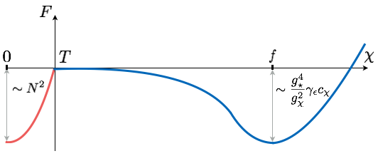
Figure 10: Schematic shape of the free energy as a function of the dilaton expectation value $\chi$. Red, hot region with $g_{\chi}\chi\lesssim T$; blue, cold region with $g_{\chi}\chi\gtrsim T$. From Bruggisser et al. (2018b).

The $CP$-violating imaginary parts of quark-Yukawa couplings lead to an electron EDM. Hence, the experimental EDM bounds constrain the viable parameter space of the model. Figure 11 shows contours of constant imaginary part for the top quark in the case of a glueball-like dilaton as well as a mesonlike dilaton. The most stringent bounds from the ACME experiment read

$$\begin{split}\text{ACME~{}(2014)}:\text{Im}[\delta\lambda_{t}]&\lesssim 2\cdot 10^{-2}\ ,\\ \text{ACME~{}(2018)}:\text{Im}[\delta\lambda_{t}]&\lesssim 2\cdot 10^{-3}\ .\end{split}$$ (65)

For a large number of hypercolors, $N=12$, corresponding to resonance masses $m_{*}\gtrsim 3~{}\text{TeV}$, a mesonlike (glueball-like) dilaton has to be heavier than $200~{}\text{GeV}$ ($400~{}\text{GeV}$). Both scenarios can therefore be probed at the LHC. Note that the effect of the ACME EDM bound on the Higgs sector can be efficiently described by means of an effective field theory (Panico, Pomarol, and Riembau, 2019).

Figure 11: Contours of the $CP$-violating imaginary part of the top-Yukawa coupling in the $(m_{\chi},m_{\star})$ plane. The dashed lines correspond to a mesonlike dilaton, and the solid lines correspond to a glueball-like dilaton. From Bruggisser et al. (2018b).

The strong constraints from the LHC and the electron EDM give rise to the question whether EWBG can be decoupled from low-energy physics. Extending the scalar sector of the theory, it is indeed possible to break the electroweak symmetry at a scale much higher than the Fermi scale (Baldes and Servant, 2018; Glioti, Rattazzi, and Vecchi, 2019; Meade and Ramani, 2019). In this way, $CP$ violation in EWBG is decoupled from low-energy $CP$ violation. On the other hand, the need to connect the high-scale vacuum expectation value to the Fermi scale requires additional light scalars that are in reach of the LHC. Similarly, additional light singlet fermions can lead to electroweak symmetry nonrestoration at high temperatures. This can significantly relax the upper bound from successful baryogenesis on a light dilaton in composite Higgs models Matsedonskyi and Servant (2020).

III.5 Summary: Electroweak baryogenesis

Electroweak baryogenesis is an appealing idea since it would allow to connect the cosmological matter-antimatter asymmetry with physics at the LHC and, moreover, with gravitational waves. The electroweak phase-transition and sphaleron processes are by now well understood. Since in the standard model the phase transition is a smooth crossover, extensions such as two-Higgs-doublet models or doublet-singlet models are needed for electroweak baryogenesis. Results from the LHC strongly constrain such models. Moreover, recent stringent upper bounds on the electron electric dipole moment exclude most of the known models. This led to the construction of models, where $CP$ violation in baryogenesis and low-energy $CP$ violation are decoupled, and the electroweak phase transition takes place at temperatures well above a TeV. On the other hand, in strongly coupled composite Higgs models electroweak baryogenesis is still possible, which is compatible with all constraints from the LHC and low-energy precision experiments. This underlines the importance of searching for new heavy resonances and deviations from SM predictions for Higgs couplings in the next run of the LHC.

IV Leptogenesis

In this section we first give an elementary introduction to the basics of leptogenesis, namely, lepton-number violation and kinetic equations. We then review thermal leptogenesis at the GUT scale as well as the weak scale. Sterile-neutrino oscillations allow leptogenesis even at GeV energies. Subsequently, we discuss recent progress toward a full quantum field-theoretical description of leptogenesis. GUT-scale leptogenesis is closely related to neutrino masses and mixings and, on the cosmological side, it is connected with inflation and gravitational waves.

IV.1 Lepton-number violation

The SM contains only left-handed neutrinos, and $B-L$ is a conserved global symmetry. Hence, in the SM neutrinos are massless. However, neutrino oscillations show evidence for nonzero neutrino masses. These can be accounted for by introducing right-handed neutrinos that can have Yukawa couplings with left-handed neutrinos. After electroweak symmetry breaking these couplings lead to $B-L$ conserving Dirac neutrino mass terms. As SM singlets, right-handed neutrinos can have Majorana mass terms whose size is not constrained by the electroweak scale. In the case of three right-handed neutrinos, the global $B-L$ symmetry can be gauged such that the Majorana masses result from the spontaneous breaking of $B-L$. As in the SM, all masses are then generated by the spontaneous breaking of local symmetries, which is the natural picture in theories that unify strong and electroweak interactions. Since no $B-L$ gauge boson has been observed thus far, the scale of $B-L$ breaking must be significantly larger than the electroweak scale. This leads to the seesaw mechanism (Minkowski, 1977; Yanagida, 1979; Gell-Mann, Ramond, and Slansky, 1979; Ramond, 1979) as a natural explanation of the smallness of the observed neutrino mass scale, which is a key element of leptogenesis.

We now consider an extension of the standard model with three right-handed neutrinos, whose masses and couplings are described by the following Lagrangian (sum over $i,j$):

$$\mathcal{L}= \overline{l_{L}}_{i}i\cancel{D}l_{Li}+\overline{e_{R}}_{i}i\cancel{D}e_{Ri}+\overline{\nu_{R}}_{i}i\cancel{\partial}\nu_{Ri}$$ (66)

$$-\big{(}h^{e}_{ij}\overline{e_{R}}_{j}l_{Li}\tilde{\phi}+h^{\nu}_{ij}\overline{\nu_{R}}_{j}l_{Li}\phi+\frac{1}{2}M_{ij}\overline{\nu_{R}}_{j}\nu_{Ri}^{c}+\text{h.c.}\big{)},$$

where $\cancel{D}$ denotes SM covariant derivatives, $\nu_{R}^{c}=C\bar{\nu}_{R}^{T}$, $C$ is the charge conjugation matrix and $\widetilde{\phi}=i\sigma_{2}\phi^{*}$. The vacuum expectation value of the Higgs field ($\langle\phi\rangle=v_{\text{E}W}$) generates Dirac mass terms $m_{e}=h^{e}v_{\text{E}W}$ and $m_{D}=h^{\nu}v_{\text{E}W}$ for charged leptons and neutrinos, respectively. Integrating out the heavy neutrinos $\nu_{R}$, the light-neutrino Majorana mass matrix becomes

$$m_{\nu}=-m_{D}\frac{1}{M}m^{T}_{D}\ .$$ (67)

The symmetric mass matrix is diagonalized by a unitary matrix $V$:

$$V^{T}m_{\nu}V=\begin{pmatrix}m_{1}&0&0\\ 0&m_{2}&0\\ 0&0&m_{3}\end{pmatrix}\ ,$$ (68)

where $m_{1}$, $m_{2}$, and $m_{3}$ are the three mass eigenvalues. In the following we mostly consider the case of normal ordering, where $m_{1}<m_{2}<m_{3}$. A recent global analysis found for the

Figure 12: Tree-level and one-loop diagrams contributing to heavy-neutrino decays

largest and smallest splitting Esteban et al. (2019)

$$\begin{split}m_{\text{atm}}&\equiv\sqrt{|m_{3}^{2}-m_{1}^{2}|}=49.9\pm 0.3\ \text{meV}\ ,\\ m_{\text{sol}}&\equiv\sqrt{|m_{2}^{2}-m_{1}^{2}|}=8.6\pm 0.1\ \text{meV}\ .\end{split}$$ (69)

The Majorana mass matrix $M$ can be chosen diagonal such that the light and heavy Majorana neutrino mass eigenstates are

$$\nu\simeq V^{T}\nu_{L}+\nu_{L}^{c}V^{*}\ ,\quad N\simeq\nu_{R}+\nu_{R}^{c}\ .$$ (70)

In a basis where the charged lepton matrix $m_{e}$ and the Majorana mass matrix $M$ are diagonal, $V$ is the Pontecorvo-Maki-Nakagawa-Sakata matrix in the leptonic charged current. $V$ can be written as $V=V_{\delta}~{}\text{diag}(1,e^{i\alpha},e^{i\beta})$, where $V_{\delta}$ contains the Dirac $CP$-violating phase $\delta$ and $\alpha$ and $\beta$ are Majorana phases.

Treating in the Lagrangian (66) the Yukawa coupling $h^{\nu}$ and the Majorana masses $M$ as free parameters, nothing can be said about the values of the light-neutrino masses. Hence, it is remarkable that the correct order of magnitude is naturally obtained in GUT models. The running of the SM gauge couplings points to a unification scale $\Lambda_{\text{GUT}}\sim 10^{15}~{}\text{GeV}$. At this scale the GUT group containing U(1)_B-L is spontaneously broken and large Majorana masses are generated ($M\propto v_{B-L}\sim 10^{15}~{}\text{GeV}$). As in the SM, all masses are now caused by spontaneous symmetry breaking. With Yukawa couplings in the neutrino sector having a similar pattern as quarks and charged leptons, with the largest values being $\mathcal{O}(1)$, one obtains for the largest light-neutrino mass

$$m_{3}\sim\frac{v^{2}_{\text{EW}}}{v_{B-L}}\sim 0.01~{}\text{eV}\ ,$$ (71)

which is qualitatively consistent with the measured value $m_{\text{atm}}$.

The tree-level decay width of the heavy Majorana neutrino $N_{i}$ reads

$$\Gamma^{0}_{N_{i}}=\Gamma^{0}(N_{i}\rightarrow l\phi)+\Gamma^{0}(N_{i}\rightarrow\bar{l}\bar{\phi})=\frac{(h^{\nu\dagger}h^{\nu})_{ii}}{8\pi}M_{i},$$ (72)

and the $CP$ asymmetry in the decay is defined as

$$\varepsilon_{i}=\frac{\Gamma(N_{i}\rightarrow l\phi)-\Gamma(N_{i}\rightarrow\bar{l}\bar{\phi})}{\Gamma(N_{i}\rightarrow l\phi)+\Gamma(N_{i}\rightarrow\bar{l}\bar{\phi})}\ .$$ (73)

We are often interested in the case of hierarchical Majorana masses $M_{2,3}\gg M_{1}\equiv M$. One can then integrate out $N_{2}$ and $N_{3}$, which yields the following effective Lagrangian for $N_{1}\equiv N$:

$$\begin{split}\mathcal{L}=&\frac{1}{2}\overline{N}i\cancel{\partial}N-h^{\nu}_{i1}N^{T}Cl_{Li}\phi-\frac{1}{2}MN^{T}CN\\ &+\frac{1}{2}\eta_{ij}l_{Li}^{T}\phi Cl_{Lj}\phi+\text{H.c.}\ ,\end{split}$$ (74)

where $\eta$ is the dimension-5 coupling

$$\eta_{ij}=\sum_{k=2,3}h^{\nu}_{ik}\frac{1}{M_{k}}h_{kj}^{\nu T}\ .$$ (75)

Using this effective Lagrangian provides the advantage that vertex- and self-energy contributions to the $CP$ asymmetry in the heavy-neutrino decay are obtained from a single Feynman diagram; see Sec. IV.6.

A nonvanishing $CP$ asymmetry in $N_{i}$ decays arises at one-loop order. From Fig. 12 one obtains (Covi, Roulet, and Vissani, 1996; Flanz, Paschos, and Sarkar, 1995),

$$\varepsilon_{i}=-\frac{1}{8\pi}\sum_{i\neq k}\frac{\text{Im}\big{(}h^{\nu\dagger}h^{\nu}\big{)}^{2}_{ik}}{\big{(}h^{\nu\dagger}h^{\nu}\big{)}_{ii}}\ F\left(\frac{M_{k}^{2}}{M_{i}^{2}}\right)\ .$$ (76)

In the case of hierarchical heavy neutrinos one obtains

$$F\left(\frac{M_{k}^{2}}{M_{i}^{2}}\right)\simeq-\frac{3}{2}\frac{M_{i}}{M_{k}}\ ,$$ (77)

and the $CP$ asymmetry can be written as

$$\varepsilon_{i}=-\frac{3}{16\pi}\frac{M_{i}}{v^{2}_{\text{EW}}\big{(}h^{\nu\dagger}h^{\nu}\big{)}_{ii}}\text{Im}\big{(}h^{\nu\dagger}m_{\nu}h^{\nu*}\big{)}_{ii}\ .$$ (78)

For small mass differences, $|M_{i}-M_{k}|\ll M_{i}+M_{k}$, the $CP$ asymmetry is dominated by the self-energy contribution in Fig. 12 and enhanced (Covi, Roulet, and Vissani, 1996):

$$F\left(\frac{M_{k}^{2}}{M_{i}^{2}}\right)\simeq-\frac{M_{i}M_{k}}{M^{2}_{k}-M_{i}^{2}}\ .$$ (79)

Once mass differences become of the order of the decay widths, one reaches a resonance regime Covi and Roulet (1997); Pilaftsis (1997) where resummations are necessary.

Thus far we have considered the seesaw mechanism with right-handed neutrinos, often referred to as the type-I seesaw. Alternatively, light-neutrino masses can result from couplings to heavy SU(2) triplet fields Mohapatra and Senjanovic (1980); Lazarides et al. (1981); Mohapatra and Senjanovic (1981); Wetterich (1981), which is referred to as the type-II seesaw. In this case the complete light-neutrino mass matrix reads

$$m_{\nu}=-m_{D}\frac{1}{M}m^{T}_{D}+m_{\nu}^{\text{triplet}}\ .$$ (80)

Such matrices are obtained in left-right symmetric extensions of the standard model; for a review, see Mohapatra and Smirnov (2006). Furthermore, one can consider the exchange of heavy SU(2) triplet fermions, which is referred to as the type-III seesaw Foot et al. (1989).

In addition to the Majorana mass matrix $M$ the charged lepton mass matrix $m_{e}=h^{e}v_{\text{E}W}$ can be chosen diagonal and real without loss of generality. The Dirac neutrino mass matrix $m_{D}$ is then a general complex matrix with nine complex parameters and therefore nine possible $CP$-violating phases. Three of these phases can be absorbed into the lepton doublets $l_{L}$, and hence six $CP$-violating phases remain physical. These are known as high-energy phases, and the $CP$ asymmetries $\varepsilon_{i}$ in $N_{i}$ decays depend on these phases. The light-neutrino mass matrix is symmetric, with six complex parameters. As before, three of the phases can be absorbed into the lepton doublets $l_{L}$, so three phases are physical: the Dirac phase $\delta$ that is measured in neutrino oscillations and two Majorana phases $\alpha_{1,2}$ that affect the rate for neutrinoless double-$\beta$ decay (Bilenky, Hosek, and Petcov, 1980; Schechter and Valle, 1980). There is no direct link between the high-energy and low-energy $CP$-violating phases, but interesting connections exist in particular models (Branco, Felipe, and Joaquim, 2012a).

IV.2 Kinetic equations

Thermal leptogenesis is an intricate nonequilibrium process in the hot plasma in the early Universe that involves decays, inverse decays, and scatterings of heavy Majorana neutrinos $N$, left-handed leptons $l$ and $\bar{l}$, complex Higgs scalars $\phi$ and $\bar{\phi}$, gauge bosons, and quarks. A key role is played by weakly coupled heavy Majorana neutrinos. In the expanding Universe they first reach thermal equilibrium and then fall out of thermal equilibrium, such that $CP$- and lepton-number-violating processes lead to a lepton asymmetry and, via sphaleron processes, also a baryon asymmetry.

The main ingredients of the nonequilibrium process can be understood by considering a simple set of Boltzmann equations, neglecting the differences between Bose-Einstein and Fermi-Dirac distribution functions, as in classical GUT baryogenesis Kolb and Turner (1990); Kolb and Wolfram (1980); Harvey et al. (1982). Relativistic corrections and a full quantum field-theoretical treatment are discussed in Sec. IV.6. For simplicity, we restrict ourselves in the following to hierarchical heavy neutrinos where the lightest one ($N$) with mass $M$ dominates leptogenesis. We also sum over lepton flavors in $N$ decays (one-flavor approximation).

We assume that at high temperatures $T\gg M$ the heavy neutrinos are in thermal equilibrium, i.e.,

$$n_{N}=\tfrac{3}{4}n_{\gamma}\ ,$$ (81)

where $n_{\gamma}$ is the photon number density, and the factor $3/4$ reflects the difference between the Bose and Fermi statistics. The heavy neutrinos decay at a temperature $T_{d}$, which is determined by $\Gamma_{N}\sim H(T_{d})$, where $\Gamma_{N}$ and $H$ are the decay width and Hubble parameter, respectively. For leptogenesis one has $T_{d}\lesssim M$ and the number density $n_{N}(T_{d})$ slightly exceeds the equilibrium number density. This departure from thermal equilibrium, together with the $CP$-violating partial decay widths [see Eq. (73)], leads to the lepton asymmetry

$$\frac{n_{l}-n_{\bar{l}}}{n_{\gamma}}=\varepsilon\frac{n_{N}}{n_{\gamma}}\sim\frac{3}{4}\varepsilon\ .$$ (82)

More realistically, one has to include inverse decays $l\phi,\bar{l}\bar{\phi}\rightarrow N$ in the calculation of the asymmetry. In general, the time evolution of a system is governed by reaction densities. i.e., the number of reactions $a+b+\ldots\rightarrow c+d+\ldots$ per time and volume:

$$\gamma(a+b+\ldots\rightarrow c+d+\cdots)=$$ (83)

$$\int d\Phi f_{a}(p_{a})f_{b}(p_{b})\ldots|\mathcal{M}(a+b+\ldots\rightarrow c+d+\ldots)|^{2},$$

where in first approximation $\mathcal{M}$ is a zero-temperature $S$-matrix element and

$$d\Phi=\frac{d^{3}p_{a}}{(2\pi)^{3}2E_{a}}\ldots(2\pi)^{4}\delta^{4}(p_{a}+\cdots-p_{c}-\ldots)$$ (84)

is the phase-space volume element. Important thermal and quantum corrections to Eq. (83) are discussed in Sec. IV.6.

It turns out that in the considered scenario kinetic equilibrium is a good approximation. In this case the distribution functions differ from the corresponding equilibrium distribution functions only by the normalization:

$$f_{a}(p)=\frac{n_{a}}{n^{\text{eq}}_{a}}f_{a}^{\text{eq}}(p)\ ,$$ (85)

and reaction densities are proportional to equilibrium reaction densities,

$$\gamma(N\rightarrow l\phi)=\frac{n_{N}}{n_{N}^{\text{eq}}}\gamma^{\text{eq}}(N\rightarrow l\phi)\ .$$ (86)

Taking the expansion of the Universe into account, one then obtains for the change of the heavy-neutrino number density with time

$$\dot{n}_{N}+3Hn_{N}= -\frac{n_{N}}{n_{N}^{\text{eq}}}[\gamma^{\text{eq}}(N\rightarrow l\phi)+\gamma^{\text{eq}}(N\rightarrow\bar{l}\bar{\phi})]$$

$$+\gamma^{\text{eq}}(l\phi\rightarrow N)+\gamma^{\text{eq}}(\bar{l}\bar{\phi}\rightarrow N)\ .$$ (87)

The reaction densities for neutrino decays into $CP$-conjugate final states differ by the $CP$ asymmetry $\varepsilon$:

$$\begin{split}\gamma^{\text{eq}}(N\rightarrow l\phi)&=\frac{1+\varepsilon}{2}\gamma_{N}\ ,\\ \gamma^{\text{eq}}(N\rightarrow\bar{l}\bar{\phi})&=\frac{1-\varepsilon}{2}\gamma_{N}\ ,\end{split}$$ (88)

and the reaction densities for decays and inverse decays are related by $CPT$ invariance:

$$\begin{split}\gamma^{\text{eq}}(\bar{l}\bar{\phi}\rightarrow N)&=\gamma^{\text{eq}}(N\rightarrow l\phi)\ ,\\ \gamma^{\text{eq}}(l\phi\rightarrow N)&=\gamma^{\text{eq}}(N\rightarrow\bar{l}\bar{\phi})\ .\end{split}$$ (89)

Together with Eq. (IV.2), Eq. (89) yields the kinetic equation for the heavy-neutrino number density:

$$\dot{n}_{N}+3Hn_{N}=-\left(\frac{n_{N}}{n_{N}^{\text{eq}}}-1\right)\gamma_{N}.$$ (90)

Integrating Eq. (90) yields the time dependence of the $N$-number density, which is determined by the expansion of the Universe and the departure from thermal equilibrium.

Figure 13: Decays and inverse decays of heavy neutrinos, $\Delta L=2$ processes with virtual intermediate heavy neutrinos, and $\Delta L=1$ scattering processes.

The lepton asymmetry is generated by heavy-neutrino decays and inverse decays as well as $2\rightarrow 2$ processes (see Fig. 13) with reaction densities such as

$$\gamma(l\phi\rightarrow\bar{l}\bar{\phi})=\int d\Phi f_{l}(p_{1})f_{\phi}(p_{2})|\hat{\mathcal{M}}(l\phi\rightarrow\bar{l}\bar{\phi})|^{2}\ .$$ (91)

Here $\hat{\mathcal{M}}$ is the matrix element for $l\phi\rightarrow\bar{l}\bar{\phi}$, from which the contribution of $N$ as the real intermediate state (RIS) has been subtracted since this is already accounted for by decays and inverse decays. Neglecting the effects of Fermi and Bose statistics the distribution functions can be approximated as

$$f_{l,\phi}(p)=\frac{n_{l,\phi}}{n^{\text{eq}}_{l,\phi}}f^{\text{eq}}_{l,\phi}(p)\simeq\frac{n_{l,\phi}}{n^{\text{eq}}_{l,\phi}}e^{-\beta[E(p)-\mu_{l,\phi}]}\ ,$$ (92)

where $\mu_{l}$ and $\mu_{\phi}$ are the chemical potentials of the lepton and the Higgs boson, respectively. The change of the lepton-number density with time is given by

$$\begin{split}\dot{n}_{l}+3Hn_{l}&=\frac{n_{N}}{n_{N}^{\text{eq}}}\gamma^{\text{eq}}(N\rightarrow l\phi)-\frac{n_{l}}{n_{l}^{\text{eq}}}\gamma^{\text{eq}}(l\phi\rightarrow N)\\ &+\frac{n_{\bar{l}}}{n_{\bar{l}}^{\text{eq}}}\gamma^{\text{eq}}(\bar{l}\bar{\phi}\rightarrow l\phi)-\frac{n_{l}}{n_{l}^{\text{eq}}}\gamma^{\text{eq}}(l\phi\rightarrow\bar{l}\bar{\phi}).\end{split}$$ (93)

The corresponding equation for $n_{\bar{l}}$ is obtained by interchanging $l,\phi$ with $\bar{l},\bar{\phi}$. An important property of the decay and scattering processes in the plasma is the unitarity of the zero-temperature $S$ matrix,

$$\sum_{i}[|\mathcal{M}(l\phi\rightarrow i)|^{2}-|\mathcal{M}(i\rightarrow l\phi)|^{2}]=0\ .$$ (94)

For $i=l^{\prime}\phi^{\prime},\bar{l}\bar{\phi}$ with $E_{l}+E_{\phi}=E_{l^{\prime}}+E_{\phi^{\prime}}=E_{\bar{l}}+E_{\bar{\phi}}$, this implies

$$\sum_{l\phi,\bar{l}\bar{\phi}}[|\mathcal{M}(l\phi\rightarrow\bar{l}\bar{\phi})|^{2}-|\mathcal{M}(\bar{l}\bar{\phi}\rightarrow l\phi)|^{2}]=0\ .$$ (95)

Expressing the lepton-number densites in terms of the $B-L$ number density

$$n_{l}=n_{l}^{\text{eq}}-\tfrac{1}{2}n_{B-L}\ ,\quad n_{\bar{l}}=n_{l}^{\text{eq}}+\tfrac{1}{2}n_{B-L}\ ,$$ (96)

one obtains from Eqs. (93) and (95) the following kinetic equation for the $B-L$ density:

$$\dot{n}_{B-L}+3Hn_{B-L}=-\varepsilon\left(\frac{n_{N}}{n_{N}^{\text{eq}}}\\ -1\right)\gamma_{N}-\frac{1}{2}\frac{n_{B-L}}{n_{l}^{\text{eq}}}\gamma_{N}\ .$$ (97)

The generation of the $B-L$ asymmetry is driven by the departure of the heavy neutrinos from equilibrium and the $CP$ asymmetry $\varepsilon$, and inverse decays also cause a washout of an existing $B-L$ asymmetry. Note that only the reaction density for $N$ decays enters into Eq. (97); the reaction density for the two-to-two process in Eq. (93) drops out.

An important part of the $B-L$ washout is the $\Delta L=2$ processes $ll\rightarrow\phi\phi$ and $l\phi\rightarrow\bar{l}\bar{\phi}$ with RIS subtracted reaction densities

$$\begin{split}\gamma^{\text{eq}}_{\text{sub}}(l\phi\rightarrow\bar{l}\bar{\phi})&=\gamma_{\Delta L=2,+}+\tfrac{1}{2}\varepsilon\gamma_{N}\ ,\\ \gamma^{\text{eq}}_{\text{sub}}(\bar{l}\bar{\phi}\rightarrow l\phi)&=\gamma_{\Delta L=2,+}-\tfrac{1}{2}\varepsilon\gamma_{N}\ ,\\ \gamma^{\text{eq}}(ll\rightarrow\bar{\phi}\bar{\phi})&=\gamma^{\text{eq}}(\bar{l}\bar{l}\rightarrow\phi\phi)=\gamma_{\Delta L=2,t}\ .\end{split}$$ (98)

When one includes the $\Delta L=2$ washout processes, the kinetic equation for the $B-L$ asymmetry becomes

$$\begin{split}\dot{n}_{B-L}+3Hn_{B-L}=&-\varepsilon\left(\frac{n_{N}}{n_{N}^{\text{eq}}}-1\right)\gamma_{N}\\ &-\frac{n_{B-L}}{n_{l}^{\text{eq}}}\left(\frac{1}{2}\gamma_{N}+\gamma_{\Delta L=2}\right)\ ,\end{split}$$ (99)

where $\gamma_{\Delta L=2}=2\gamma_{\Delta L=2,+}+2\gamma_{\Delta L=2,t}$. Note that the full Boltzmann equation for the number density $n_{B-L}$ also depends on the number densities of charged leptons, quarks, and Higgs boson, which satisfy their own Boltzmann equations. The corresponding chemical potentials are all coupled by the sphaleron processes. A discussion of such “spectator processes” can be found in Sec. IV.6 and in Buchmuller and Plumacher (2001), Nardi et al. (2006a), and Garbrecht and Schwaller (2014). They can affect the final $B-L$ asymmetry by a factor of $\mathcal{O}(1)$.

Early studies of leptogenesis were partly motivated by trying to find alternatives to electroweak baryogenesis, which did not seem to produce a large enough asymmetry. Several extensions of the standard model with hierarchical heavy-neutrino masses were found that could explain the observed value of the baryon asymmetry (Langacker, Peccei, and Yanagida, 1986; Luty, 1992; Gherghetta and Jungman, 1993) At that time models with keV-scale light neutrinos were still considered. After washout processes were correctly taken into account, it was realized that for hierarchical mass matrices inspired by SO(10) GUTs neutrino masses below $1~{}\text{eV}$ were favored Buchmuller and Plumacher (1996) Subsequently, atmospheric neutrino oscillations were discovered, which led to a strongly rising interest in leptogenesis and a large number of interesting models; for reviews and references, see Mohapatra and Smirnov (2006) and Altarelli and Feruglio (2010). The minimal seesaw model for leptogenesis contains two right-handed neutrinos (Frampton, Glashow, and Yanagida, 2002). This class of models was recently reviewed by Xing and Zhao (2020).

IV.3 Thermal leptogenesis

IV.3.1 One-flavor approximation

To understand the nonequilibrium process of thermal leptogenesis one has to compare the reaction rates per particle with the Hubble parameter as a function of temperature or, more conveniently, $z=M/T$. The decay and washout rates are obtained by dividing the reaction densities by the relevant equilibrium number densities:

$$\Gamma_{N}=\frac{1}{n_{N}^{\text{eq}}}\gamma_{N}\ ,\quad\Gamma_{W}=\frac{1}{n_{l}^{\text{eq}}}\left(\frac{1}{2}\gamma_{N}+\gamma_{\Delta L=2}\right)\ .$$ (100)

At low temperatures ($z>1$), decays and inverse decays dominate $N$ production and $B-L$ washout, whereas at high temperatures ($z<1$) $2\rightarrow 2$ scatterings with rate $\Gamma_{S}$ are equally important; see Fig. 13 and Sec. IV.6 for details. All rates have to be evaluated as functions of $z$ by performing a thermal average over the corresponding matrix elements Luty (1992); Plumacher (1997); Biondini et al. (2018). They are compared to the Hubble parameter in the upper panel of Fig. 14. For $z<1$, all processes are out of thermal equilibrium ($\Gamma_{D,W,S}<H$). Around $z\sim 1$, the various processes come into thermal equilibrium. Heavy neutrinos now decay and, since their number density slightly exceeds the equilibrium number density, a $B-L$ asymmetry is generated in these decays. As long as washout processes are in equilibrium, the asymmetry is partly washed out again. At $z>1$, $N$ production is kinematically suppressed, the washout processes eventually get out of equilibrium at some $z_{L}$, and the $B-L$ asymmetry is frozen in.

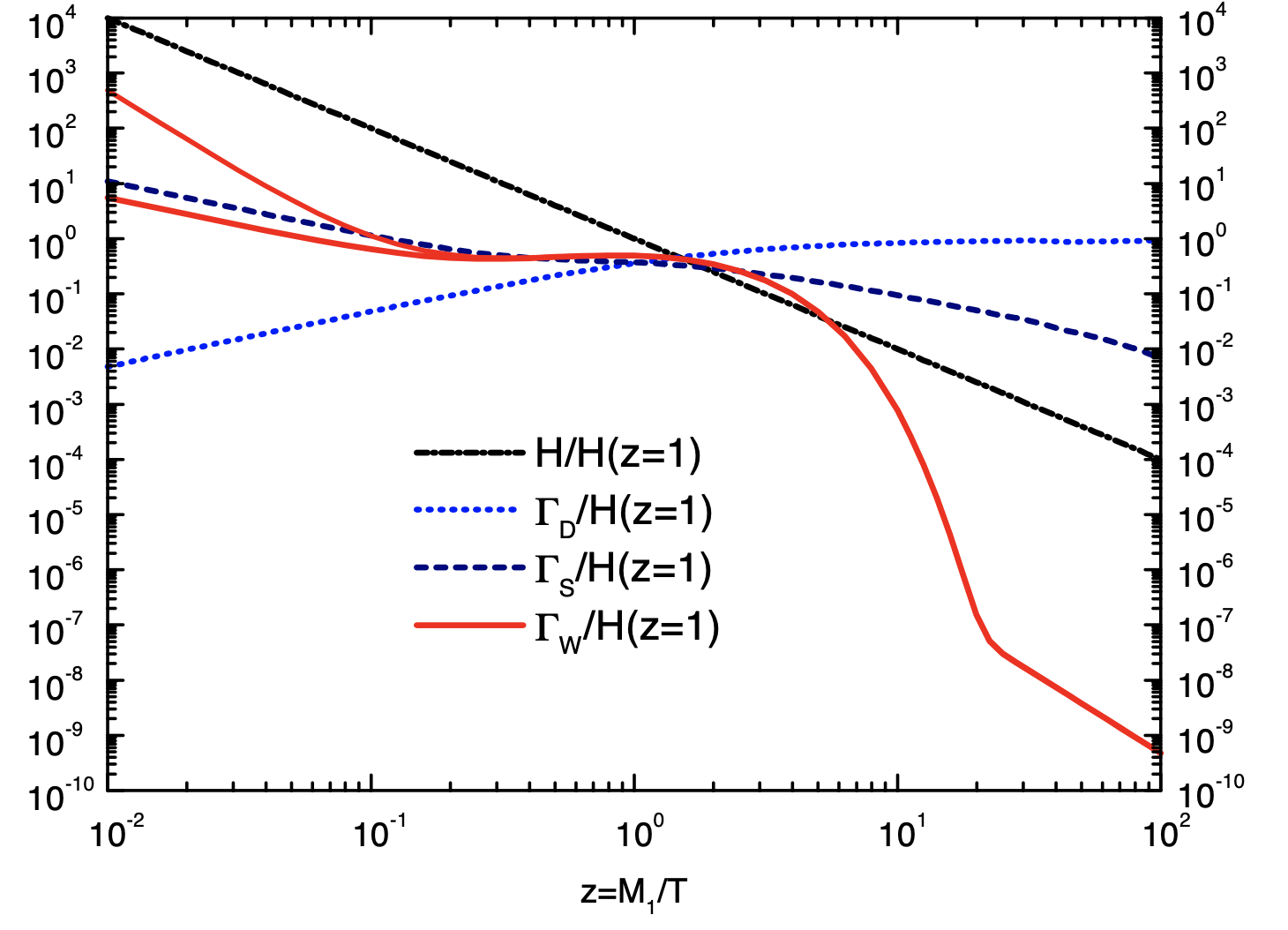
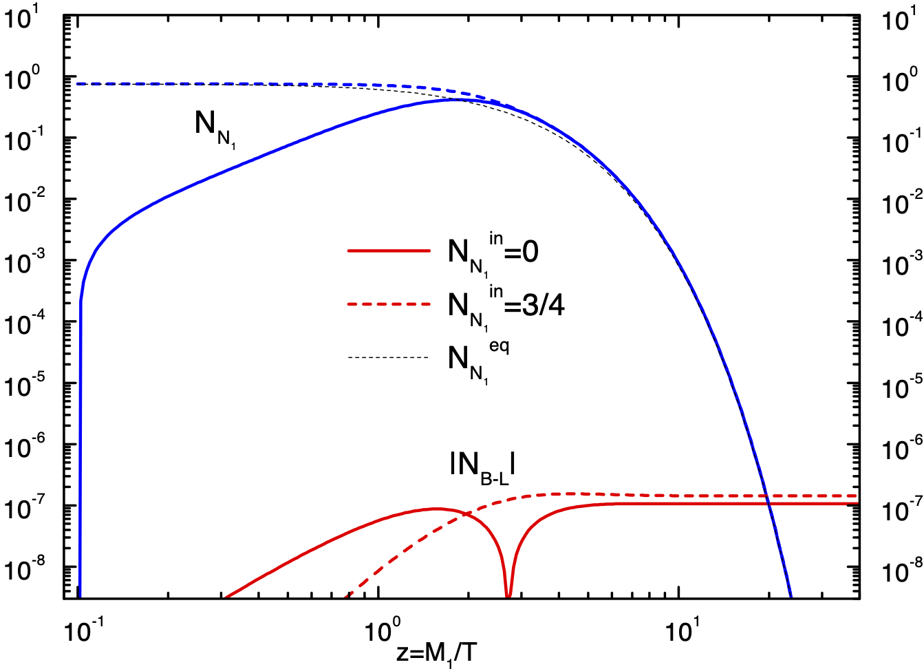
Figure 14: Top panel: decay, scattering and washout rates normalized to the Hubble parameter at $z=1$ compared to the Hubble parameter $H(z)$. The two branches of $\Gamma_{W}$ at $z\ll 1$ represent approximate upper and lower bounds. Bottom panel: evolution of $N_{1}$ abundance and $B-L$ asymmetry for both thermal and zero initial abundance. The neutrino parameters are $M_{1}=10^{10}~{}\text{GeV}$, $\widetilde{m}_{1}=10^{-3}~{}\text{GeV}$, and $\bar{m}=0.05~{}\text{GeV}$. From Buchmuller, Di Bari, and Plumacher (2002b).

In the kinetic equations (90) and (99) the Hubble parameter appears. It is convenient to separate the time dependence of the leptogenesis process from the expansion of the Universe. This can be achieved by considering the ratio of a number density $n_{X}$ to the entropy density $Y_{X}=n_{X}/s$, or the product of $n_{X}$ and the comoving volume occupied by one particle, such as a photon, i.e., $N_{X}=2n_{X}/n_{\gamma}$, at some time before the onset of leptogenesis. For the standard model in the high-temperature phase, assuming one relativistic heavy-neutrino species, one has $s=217\pi^{4}/[90\zeta(3)]n_{\gamma}$ Kolb and Turner (1990), and therefore

$$Y_{X}(z)=\frac{45\zeta(3)}{217\pi^{4}}N_{X}(z)\ ,\quad z<1\ .$$ (101)

Changing variables and defining the rescaled reaction rates $D=\Gamma_{N}/Hz$ and $W=\Gamma_{W}/Hz$, the kinetic equations (90) and (99) take the simple form

$$\begin{split}\frac{dN_{N}}{dz}&=-D(N_{N}-N_{N}^{\text{eq}})\ ,\\ \frac{dN_{B-L}}{dz}&=-\varepsilon D(N_{N}-N^{\text{eq}})-WN_{B-L}\ .\end{split}$$ (102)

The maximal $B-L$ asymmetry to which leptogenesis can lead is determined by the $CP$ asymmetry in $N$ decays out of equilibrium, as described by Eq. (82). The coupling of the heavy neutrinos to the thermal bath implies a suppression of the final asymmetry $N_{B-L}^{\text{f}}=N_{B-L}(z\gg 1)$, which is expressed in terms of an efficiency factor $\kappa$ Barbieri et al. (2000) as

$$N_{B-L}^{\text{f}}=-\tfrac{3}{4}\varepsilon\kappa_{\text{f}}\ ,$$ (103)

where the factor $3/4$ is taken from the Fermi statistics. During the evolution of the Universe the $B-L$ asymmetry in a comoving volume element remains constant, whereas the number of photons increases. The measured baryon-to-photon ratio at recombination is then given by

$$\eta_{B}=\frac{n_{B}}{n_{\gamma}}=\frac{3}{4}\frac{c_{s}}{f}\varepsilon\kappa_{\text{f}}\simeq\eta_{B}\simeq 0.96\times 10^{-2}\varepsilon\kappa_{\text{f}}\ .$$ (104)

Here $c_{s}$ is the fraction of $B-L$ asymmetry converted into a baryon asymmetry by sphaleron processes [see Eq. (39)], and the dilution factor $f$ is the increase of the number of photons in a comoving volume element. In the standard model with one heavy neutrino one has $c_{s}=28/79$ and $f=2387/86$.

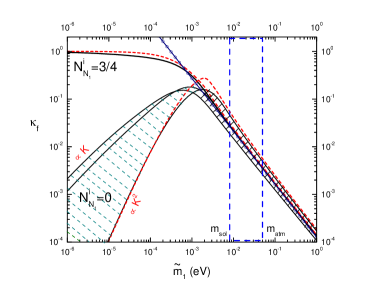
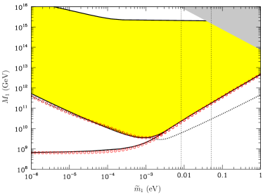
Figure 15: Left panel: efficiency factor $\kappa_{\text{f}}$ as a function of the effective neutrino mass $\widetilde{m}_{1}$. The hatched region represents the theoretical uncertainty due to $\Delta L=1$ scattering processes, the dashed lines indicate analytical results, and the circled line is a power-law fit. Right panel: upper and lower bounds on the heavy-neutrino mass $M_{1}$ (the weaker lower bound corresponds to thermal initial conditions). The dotted line is a lower bound on the initial temperature $T_{i}$; the gray triangle is excluded by theoretical consistency and the circled lines represent analytical results. In both panels the vertical lines indicate the range $(m_{\text{sol}},m_{\text{atm}})$ (see the text). From Buchmuller, Di Bari, and Plumacher (2005a).

In the upper panel of Fig. 14 decay and washout rates are depicted for a representative choice of neutrino masses. The lower panel shows solutions of the kinetic equations (102) for the same mass parameters and two different choices of initial conditions, namely, thermal and zero initial $N$ abundance. For thermal initial abundance the number $N_{N}$ always exceeds the equilibrium value $N_{N}^{\text{eq}}$, and the asymmetry $|N_{B-L}|$ continuously increases toward its final value. For zero initial abundance $N_{N}-N_{N}^{\text{eq}}$ is first negative. It changes sign just above $z=1$, where also $|N_{B-L}|$ passes through zero. For the chosen neutrino mass parameters the final $B-L$ asymmetry is almost independent of the initial condition. The value of the baryon-to-photon ratio $\eta_{B}\sim 0.01N^{\text{f}}_{B-L}$ is in agreement with observations.

The generated $B-L$ asymmetry strongly depends on neutrino parameters, and it is noteworthy that for masses and mixings consistent with neutrino oscillations the observed baryon-to-photon ratio is naturally obtained. The robustness of the leptogenesis mechanism is largly due to the fact that for neutrino masses below $0.1~{}\text{eV}$ the $B-L$ asymmetry is essentially determined only by decays and inverse decays. The heavy neutrinos decay at $z>1$, such that scattering processes are unimportant, and for small neutrino masses $\Delta L=2$ washout processes are suppressed (Buchmuller, Di Bari, and Plumacher, 2005a). Moreover, relativistic corrections are small. In the case where a summation of the lepton flavors in the final state is performed, the efficiency factor depends only on $\widetilde{m}_{1}$ and $M\bar{m}^{2}$, where the effective light-neutrino mass $\widetilde{m}_{1}$ and the absolute neutrino mass scale $\overline{m}$ are defined as

$$\widetilde{m}_{1}=\frac{(h^{\nu\dagger}h^{\nu})_{11}v^{2}_{\text{EW}}}{M_{1}}\ ,\quad\overline{m}=\sqrt{m_{1}^{2}+m_{2}^{2}+m_{3}^{2}}\ .$$ (105)

For $\overline{m}\lesssim 0.1~{}\text{eV}$ and $M\lesssim 10^{14}~{}\text{GeV}$, the efficiency factor $\kappa_{\text{f}}$ depends only on $\widetilde{m}_{1}$. As the left panel of Fig. 15 illustrates, there are two regimes, with “weak” and “strong” washout, corresponding to

$$\widetilde{m}_{1}<m_{*}\ ,\quad\widetilde{m}_{1}>m_{*}\ ,$$ (106)

respectively, where $m_{*}$ is the equilibrium neutrino mass:

$$m_{*}=\frac{16\pi^{5/2}\sqrt{g_{*}}}{3\sqrt{5}}\frac{v^{2}}{M_{\text{P}}}\simeq 1.08\times 10^{-3}~{}\text{eV}\ .$$ (107)

The ratio $\widetilde{m}_{1}/m_{*}=\Gamma_{D}(z=\infty)/H(z=1)\equiv K$ was previously introduced in GUT baryogenesis Kolb and Wolfram (1980). In the weak-washout regime $\kappa_{\text{f}}(\widetilde{m}_{1})$ strongly depends on the initial conditions (thermal versus zero initial abundance) and on the rate for $\Delta L=1$ scattering processes (the hatched area in Fig. 15). On the contrary, in the strong-washout regime the efficiency factor is universal, with an uncertainty of about 50%:

$$\kappa_{\text{f}}=(2\pm 1)\times 10^{-2}\left(\frac{0.01~{}\text{eV}}{\widetilde{m}_{1}}\right)^{1.1\pm 0.1}\ .$$ (108)

Moreover, the dependence of the final $B-L$ asymmetry on some other initial $B-L$ asymmetry, independent of leptogenesis, is significantly suppressed in the strong-washout regime. It is noteworthy that the neutrino mass range indicated by solar and atmospheric neutrinos lies inside the strong-washout regime where the generated $B-L$ asymmetry is essentially determined by decays and inverse decays and therefore largely independent of initial conditions and theoretical uncertainties.

In the case of hierarchical heavy neutrinos the maximal $CP$ asymmetry in $N$ decays reads (Davidson and Ibarra, 2002; Hamaguchi, Murayama, and Yanagida, 2002)

$$\varepsilon_{\text{max}}=\frac{3}{16\pi}\frac{Mm_{\text{atm}}}{v^{2}}\simeq 10^{-6}\left(\frac{M}{10^{10}~{}\text{GeV}}\right)\ .$$ (109)

As we know the maximal efficiency factor, Eq. (109) implies a lower bound on the smallest heavy-neutrino mass $M$. From Fig. 15 one reads off $\kappa^{\text{max}}\sim 1$ and $\kappa^{\text{max}}\sim 0.1$ for thermal and zero initial abundance, respectively. A baryon-to-photon ratio $\eta_{B}\sim 10^{-9}$ then requires a heavy-neutrino mass $M\gtrsim 10^{8}~{}\text{GeV}$ and $10^{9}~{}\text{GeV}$ for the two different initial conditions, respectively. The precise dependence of the lower bound on $\widetilde{m}_{1}$ is shown in the right panel of Fig 15.

The $\Delta L=2$ washout term leads to an upper bound on heavy-neutrino masses and also to an important upper bound on the light-neutrino masses (Buchmuller, Di Bari, and Plumacher, 2002a). An analysis of the solution of the kinetic equations (102) shows that in the strong-washout regime, which is defined by $\widetilde{m}_{1}\gtrsim m_{*}$, the $B-L$ asymmetry is produced close to $z_{B}(\widetilde{m}_{1})\sim 2m_{*}/\widetilde{m}_{1}\kappa_{\text{f}}(\widetilde{m}_{1})$, and the complete efficiency factor is given by

$$\begin{split}\bar{\kappa}_{\text{f}}&(\widetilde{m}_{1},M\overline{m}^{2})\simeq\\ &\kappa_{\text{f}}(\widetilde{m}_{1})\exp{\left[-\frac{\omega}{z_{B}}\left(\frac{M}{10^{10}~{}\text{GeV}}\right)\left(\frac{\overline{m}}{\text{eV}}\right)^{2}\right]}\ ,\end{split}$$ (110)

where $\omega\simeq 0.2$. For too large values of $M$ and $\overline{m}$, the generated $B-L$ asymmetry is too small relative to observation. A quantitative analysis yields for $M$ the upper bound shown in Fig. 15, and for the light-neutrino masses one finds $m_{i}<0.12~{}\text{eV}$. Assuming $\widetilde{m}_{1}=\mathcal{O}(m_{i})$, successful leptogenesis then implies for the light neutrinos the optimal mass window

$$10^{-3}\lesssim m_{i}\lesssim 0.1~{}\text{eV}\ .$$ (111)

It is notable that the cosmological bound on the sum of neutrino masses Aghanim et al. (2020b), which has become increasingly stringent over the past two decades, is consistent with this mass window. Note, however, that the upper bound on the light-neutrino masses holds only in type-I seesaw models. In type-II models, where a triplet contribution appears in the neutrino mass matrix as in left-right symmetric models, the direct connection between neutrino masses and leptogenesis is lost Hambye and Senjanovic (2004); Antusch and King (2004).

The maximal $CP$ asymmetry [Eq. (109)], and therefore the lower bound on the heavy-neutrino mass $M_{1}$, depends on the measured value of $m_{\text{atm}}$. What can one say without knowing the result from atmospheric neutrino oscillations? In this case the Planck mass and the Fermi scale still yield the neutrino mass scale $m_{*}$ [see Eq. (107)], which determines the normalization of $\widetilde{m}_{1}$ in the efficiency factor $\kappa_{f}$ [Eq. (108)]. From the full efficiency factor [Eq. (110)] one can then determine the maximal baryon asymetry as a function of $\widetilde{m}_{1}$ and $m_{3}$, which is reached at $\widetilde{m}_{1}\simeq 2\times 10^{-3}~{}\text{eV}$, i.e., in the strong-washout regime (Buchmuller, Di Bari, and Plumacher, 2004). This leads to the upper and lower bounds $m_{3}\lesssim 250~{}\text{eV}$ and $M_{1}\gtrsim 2\times 10^{6}~{}\text{GeV}$, respectively.

In GUTs with hierarchical heavy right-handed neutrinos ($M_{1}\ll M_{2}\ll M_{3}\sim v_{B-L}\sim 10^{15}~{}\text{GeV}$, a simple estimate yields the right order of magnitude for the baryon-to-photon ratio Buchmuller and Plumacher (1996); Buchmuller and Yanagida (1999). To understand this, consider the $CP$ asymmetry $\varepsilon_{1}$ given in Eq. (78), assume normal ordering, and keep the largest contribution proportional to the light-neutrino mass $m_{3}$. With $h^{\nu}_{i1}/\sqrt{(h^{\nu\dagger}h^{\nu})_{11}}\propto\delta_{i3}$ and using Eq. (71), one obtains

$$\varepsilon_{1}\sim 0.1\ \frac{m_{3}M_{1}}{v^{2}_{\text{EW}}}\sim 0.1\ \frac{M_{1}}{M_{3}}\ .$$ (112)

For a heavy-neutrino mass hierarchy similar to the hierarchies in the quark and charged lepton sectors, i.e., $M_{1}/M_{3}\sim 10^{-5}\cdots 10^{-4}$, and an efficiency factor $\kappa_{f}\sim 10^{-2}\cdots 10^{-1}$, the baryon-to-photon ratio is given by [see Eq. (104)],

$$\eta_{B}\sim 10^{-2}\ \varepsilon_{1}\kappa_{f}\sim 10^{-10}\cdots 10^{-8}\ ,$$ (113)

which is in agreement with observation.

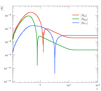
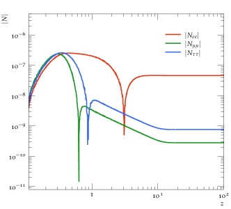
Figure 16: Evolution of the $B-L$ asymmetry for each lepton flavor as a function of $z=M_{1}/T$ for the two sets of neutrino masses and phases (left panel: $S_{2}$; right panel: $S_{3}$) listed in Table 1. From Moffat et al. (2018).

The $\Delta L=2$ washout terms play a crucial role in obtaining upper bounds on light- and heavy-neutrino masses. Correspondingly, a discovery of lepton-number-violating dilepton events at the LHC could be used to falsify leptogenesis since the production cross section of these events is directly related to a $\Delta L=2$ washout term that, if large enough, would erase any baryon asymmetry. This has been demonstrated in the context of left-right symmetric models (Frere, Hambye, and Vertongen, 2009) as well as in a model-independent approach (Deppisch, Harz, and Hirsch, 2014).

IV.3.2 Flavor effects

Thus far we have discussed leptogenesis in the “one-flavor approximation”, where one sums over lepton flavors in the final state. This approximation is valid only at high temperatures where lepton-Higgs interactions in the thermal plasma can be neglected. In general, flavor effects can have an important impact on leptogenesis Barbieri et al. (2000); Endoh et al. (2004); Abada et al. (2006); Nardi et al. (2006b); Blanchet et al. (2007).

We first consider the simplest case where the lightest heavy neutrino $N_{1}\equiv N$ couples to the following combination of lepton flavors given by the Yukawa couplings $h^{\nu}_{i1}$ [see Eq. (74)]:

$$|l_{1}\rangle=\sum_{i=e,\mu,\tau}C_{1i}|l_{i}\rangle\ ,\quad C_{1i}=\frac{h^{\nu}_{i1}}{\sqrt{(h^{\nu\dagger}h^{\nu})_{11}}}\ .$$ (114)

As the Universe expands, Hubble parameter and Yukawa rates decrease as $H\sim T^{2}/M_{\text{P}}$ and $\Gamma_{Y}\sim g_{Y}^{2}T$, respectively. Hence, with $g_{\tau}\sim 5\times 10^{-3}$, left- and right-handed $\tau$ neutrinos are in thermal equilibrium for temperatures below the temperature $T_{\tau}$, where

$$\Gamma_{\tau}(T_{\tau})\sim\frac{g_{\tau}^{2}}{4\pi}~{}T_{\tau}\sim 10^{-6}~{}T_{\tau}\sim H(T_{\tau})\ ,$$ (115)

which implies $T_{\tau}\sim 10^{12}~{}\text{GeV}$. Below $T_{\tau}$ interactions with $\tau$ leptons in the thermal bath destroy the coherence of the lepton state produced in $N$ decay. Hence, one has to consider Boltzmann equations for the components parallel and orthogonal to $\tau$ separately. With

$$p_{\tau}=|C_{1\tau}|^{2}\ ,\quad p_{\tau^{\perp}}=1-|C_{1\tau}|^{2}\ ,\quad\langle\tau|\tau^{\perp}\rangle=0\ ,$$ (116)

one obtains

$$\begin{split}\frac{dN_{N}}{dz}&=-D(N_{N}-N_{N}^{\text{eq}})\ ,\\ \frac{dN_{\tau\tau}}{dz}&=\varepsilon_{\tau\tau}D(N_{N}-N^{\text{eq}})-p_{\tau}WN_{\tau\tau}\ ,\\ \frac{dN_{\tau^{\perp}\tau^{\perp}}}{dz}&=\varepsilon_{\tau^{\perp}\tau^{\perp}}D(N_{N}-N^{\text{eq}})-p_{\tau^{\perp}}WN_{\tau^{\perp}\tau^{\perp}}\ .\end{split}$$ (117)

For the produced $B-L$ asymmetry these equations yield the flavor structure

$$N_{B-L} \propto\left(\frac{\varepsilon_{\tau\tau}}{p_{\tau\tau}}+\frac{\varepsilon_{\tau^{\perp}\tau^{\perp}}}{p_{\tau^{\perp}\tau^{\perp}}}\right)$$

$$\propto\varepsilon_{\tau\tau}\left(\frac{1}{p_{\tau\tau}}-\frac{1}{1-p_{\tau\tau}}\right)\ .$$ (118)

A complete expression for the $B-L$ asymmetry in the two-flavor regime was given by Blanchet and Di Bari (2009). For temperatures far below $T_{\tau}$ all three lepton flavors have to be taken into account. Instead of Eqs. (117) one then obtains an involved system of Boltzmann equations or, depending on the temperature regime, kinetic equations for the lepton density matrix Blanchet et al. (2013).

Flavor effects, together with tuning of the parameters of the seesaw mass matrix, can be used to lower the leptogenesis temperature significantly below $T\sim 10^{10}~{}\text{GeV}$, which was considered in the previous section Blanchet and Di Bari (2009). Recently, a detailed study of this type has been carried out by Moffat et al. (2018), who took masses and mixings of all three light and heavy Majorana neutrinos into account. A code to solve these Boltzmann equations was published by Granelli et al. (2020). Two sets of neutrino parameters, fitted to the measured neutrino parameters and the observed baryon asymmetry, are shown in Table 1. The two sets $S_{2}$ and $S_{3}$ correspond to normal hierarchy for the light neutrinos and to a mild mass hierarchy for heavy neutrinos. Mixing angles and mass ratios of the light neutrinos are essentially fixed by observation. In both cases the smallest neutrino mass lies in the mass window [Eq. (111)], whereas the Dirac phase and Majorana phases vary significantly. Correspondingly, the flavor dependence of the $B-L$ asymmetry is different in the two cases. The dependence on the mixing parameters of the heavy neutrinos is not listed. An important aspect of the flavor effects is the mass scale of the heavy neutrinos, which lies significantly below the lower bound derived in the one-flavor approximation.

Compare the evolution of the $B-L$ asymmetry in Fig. 16 to that shown in Fig. 14, where $M_{1}$, the smallest heavy-neutrino mass, is 3 orders of magnitude larger than in the parameter sets $S_{2}$ and $S_{3}$. In Fig. 14 the generated asymmetry before the thermal equilibrium of $N_{1}$ is about the same as the final $B-L$ asymmetry, whereas in Fig. 16 there is a difference of about 1 order of magnitude. The flavor composition of the $B-L$ asymmetry is significantly different for $S_{2}$ and $S_{3}$. Such a behavior can occur due to cancellations between positive and negative contributions to the asymmetry around $z\approx 1$, as discussed by (Buchmuller, Di Bari, and Plumacher, 2005a). Moreover, fine-tuning between tree-level contributions and one-loop corrections to the light-neutrino mass matrix is needed. On the whole the total $B-L$ asymmetry is rather sensitive to fine-tuning of the parameters, which is the price one pays for lowering the heavy-neutrino mass scale relative to the simple one-flavor approximation, thereby allowing for a low reheating temperature.

	$\delta(^{\circ})$	$m_{1}$ (eV)	$M_{1}$ (GeV)	$M_{2}$ (GeV)	$M_{3}$(GeV)
$S_{2}$	$88.26$	$0.079$	$10^{6.5}$	$10^{7}$	$10^{7.5}$
$S_{3}$	$31.71$	$0.114$	$10^{6.5}$	$10^{7.2}$	$10^{7.9}$

Table 1: Two sets of neutrino masses and phases consistent with the observed $B-L$ asymmetry (only 5 out of 14 parameters are listed). Adapted from Moffat et al., 2018.

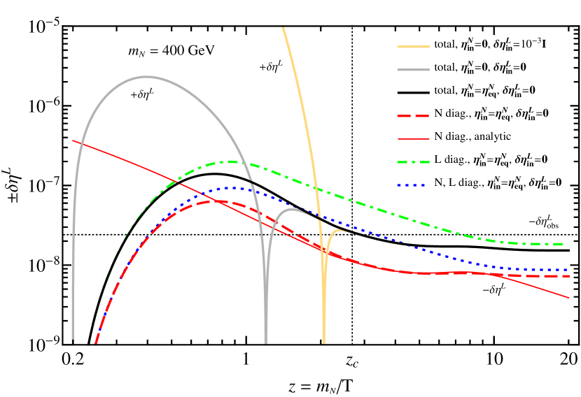
Figure 17: Resonant leptogenesis: lepton asymmetry $\eta^{L}$, with $L=L_{\tau}$, computed in a density matrix formalism for different initial conditions (solid lines), compared to $\eta^{L}$ obtained in a flavor-diagonal approximation (dashed lines). The model parameters are specified in the table. From Bhupal Dev et al. 2015.

An important aspect of the flavor dependence of leptogenesis is the effect on upper and lower bounds on light-neutrino masses. The effect can be significant, but thus far it has not been possible to obtain a complete picture in a model-independent way. According to current estimates, it is possible to relax the upper and lower bounds in Eq. (111) by about 1 order of magnitude, barring fine-tuning (Davidson et al., 2008; Blanchet and Di Bari, 2012; Dev et al., 2018b). Moreover, spectator effects have to be taken into account (Buchmuller and Plumacher, 2001; Nardi et al., 2006a; Garbrecht and Schwaller, 2014).

Our discussion of flavor effects has been limited to the case where leptogenesis is dominated by the lightest heavy neutrino $N_{1}$. An alternative is dominance by the next-to-lightest heavy neutrino $N_{2}$ Di Bari (2005); Vives (2006). More possibilities were reviewed by Dev et al. (2018b). The treatment of flavor effects based on Kadanoff-Baym equations Beneke et al. (2011) is described in Sec. IV.6.

Continuous and discrete flavor symmetries play an important role in restricting lepton masses and mixings, and in this way they strongly effect leptogenesis. This has been extensively discussed in the literature; comprehensive overviews were given by Mohapatra and Smirnov (2006) and Altarelli and Feruglio (2010).

IV.3.3 Resonant leptogenesis

The standard temperature scale of thermal leptogenesis ($T\gtrsim 10^{10}~{}\text{GeV}$) can be significantly lowered by flavor effects. A much more dramatic effect occurs when mass differences between the heavy neutrinos are comparable to the heavy-neutrino decay widths, a case referred to as resonant leptogenesis Pilaftsis and Underwood (2004). In this case leptogenesis temperatures of the order of TeV are possible, which implies the possibility of testing thermal leptogenesis at high-energy colliders Pilaftsis and Underwood (2005). Such models can be realized in extensions of the standard model where the quasidegeneracy of the heavy neutrinos is a consequence of approximate symmetries, as in supersymmetric models, where soft supersymmetry breaking terms can be much smaller than the heavy-neutrino mass terms; see D’Ambrosio, Giudice, and Raidal (2003), Grossman et al. (2003), Chen and Mahanthappa (2004), and Hambye, March-Russell, and West (2004).

The formalism to treat this resonant regime was developed in resummed perturbation theory Pilaftsis and Underwood (2004), on the basis of Kadanoff-Baym equations (Garny, Kartavtsev, and Hohenegger, 2013), and using a density matrix formalism Bhupal Dev et al. (2015); for a review, see Dev et al. (2018a). In resummed perturbation theory one computes the decay rates of heavy neutrinos $N_{\alpha}$ to leptons $l$ and the Higgs boson,

$$\Gamma_{\alpha l}=\Gamma(N_{\alpha}\rightarrow l\phi)\ ,\quad\Gamma^{C}_{\alpha l}=\Gamma(N_{\alpha}\rightarrow\overline{l}\overline{\phi})\ ,$$ (119)

in terms of resummed Yukawa couplings $\overline{\bf h}^{\nu}_{l\alpha}$ Pilaftsis and Underwood (2004). The $CP$ asymmetries are defined as usual:

$$\begin{split}\delta_{\alpha l}&\equiv\frac{\Gamma_{\alpha l}^{\phantom{C}}-\Gamma_{\alpha l}^{C}}{\sum\limits_{l=e,\mu,\tau}\Big{(}\Gamma_{\alpha l}^{\phantom{C}}+\Gamma_{\alpha l}^{C}\Big{)}}\\ &=\frac{\big{|}\overline{\bf h}^{\nu}_{l\alpha}\big{|}^{2}-\big{|}\overline{\bf h}^{\nu C}_{l\alpha}\big{|}^{2}}{\big{(}\overline{\bf h}^{\nu\dagger}\ \overline{\bf h}^{\nu\phantom{\dagger}}\!\!\big{)}_{\alpha\alpha}+\big{(}\overline{\bf h}^{\nu C\dagger}\ \overline{\bf h}^{\nu C\phantom{\dagger}}\!\!\big{)}_{\alpha\alpha}}\ .\end{split}$$ (120)

For quasidegenerate heavy neutrinos the decay rates show the typical resonant enhancement, and for two heavy neutrinos one has obtained the result Pilaftsis and Underwood (2004)

$$\begin{split}\delta_{\alpha l}\ \approx\ &\frac{{\rm Im}\big{[}({\bf h}^{\nu\dagger}_{\alpha l}{\bf h}^{\nu\phantom{\dagger}}_{l\beta})\ ({\bf h}^{\nu\dagger}_{\phantom{l}}{\bf h}^{\nu\phantom{\dagger}}_{\phantom{l}}\!\!)_{\alpha\beta}\big{]}}{({\bf h}^{\nu\dagger}_{\phantom{l}}{\bf h}^{\nu\phantom{\dagger}}_{\phantom{l}}\!\!)_{\alpha\alpha}\ ({\bf h}^{\nu\dagger}_{\phantom{l}}{\bf h}^{\nu\phantom{\dagger}}_{\phantom{l}}\!\!)_{\beta\beta}}\\ &\times\frac{(m^{2}_{N_{\alpha}}-m^{2}_{N_{\beta}})\,m_{N_{\alpha}}\,\Gamma^{(0)}_{N_{\beta}}}{(m^{2}_{N_{\alpha}}-m^{2}_{N_{\beta}})^{2}+m^{2}_{N_{\alpha}}\Gamma^{(0)2}_{N_{\beta}}}\ .\end{split}$$ (121)

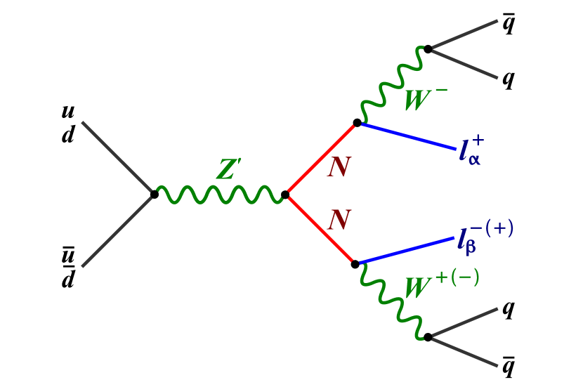
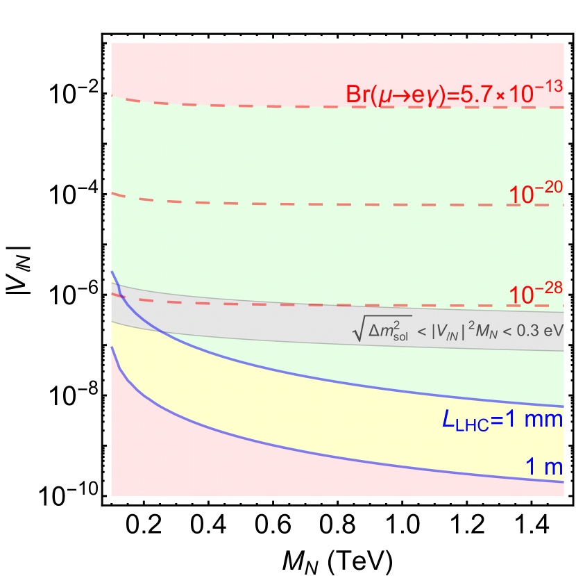
Figure 18: Left panel: heavy-neutrino pair production and decay in an extension of the standard model with an additional $Z^{\prime}$ boson. Right panel: contours in the plane of neutrino mixing $|V_{lN}|$ and neutrino mass $m_{N}$. The dashed red lines correspond to different branching ratios $\text{BR}(\mu\rightarrow e\gamma)$, and the blue lines correspond to two distances between displaced vertices at the LHC. From Deppisch, Bhupal Dev, and Pilaftsis (2015).

A numerical example is shown in Fig. 17. The lepton asymmetry is all in the $\tau$ flavor. It is notable that the mass of the three heavy neutrinos can be lowered to $m_{N}=400~{}\text{GeV}$. The price is the extreme fine-tuning of mass differences $\Delta M_{1}/m_{N}=(M_{1}-m_{N})/m_{N}\sim 10^{-5}$ and $\Delta M_{2}/m_{N}=(M_{2}-M_{3})/m_{N}\sim 10^{-9}$, with $m_{N}=(M_{2}+M_{3})/2$. As in the case discussed in the Sec. IV.3.2 (see Fig. 16), the final asymmetry $|\delta^{L}|$ is much smaller than the asymmetry $|\delta^{L}|$ before the equilibrium of the heavy neutrinos, indicating the sensitivity with respect to fine-tuning of the parameters.

Some special parameter region of resonant leptogenesis can be probed at the LHC (Deppisch, Bhupal Dev, and Pilaftsis, 2015). At zero temperature the four real degrees of freedom of the complex doublet $\phi$ become the physical Higgs $H$ and the longitudinal components of $W$ and $Z$ bosons. The heavy neutrinos can decay into these bosons and leptons with decay rates related to Eq. (119):

$$\Gamma_{\alpha l}=\Gamma(N_{\alpha}\to l^{-}_{lL}+W^{+})+\Gamma(N_{\alpha}\to\nu_{lL}+Z,H)\ .$$ (122)

To obtain a sufficiently large cross section for heavy-neutrino pair production it is necessary to extend the standard model by an additional U(1) gauge group and a corresponding $Z^{\prime}$ gauge boson. The produced heavy neutrinos then decay into $l_{L}^{\pm}W^{\mp}$ or $\nu_{L}Z,H$. This leads to interesting like-sign ($l^{+}l^{+}$) and opposite-sign ($l^{+}l^{-}$) dilepton events; see Fig. 18. The decay amplitude is proportional to the light- and heavy-neutrino mixing $|V_{lN}|\sim\sqrt{m_{\nu}/m_{N}}=\mathcal{O}(10^{-6})$. Hence, the lifetime of the decaying heavy neutrino $N$ is long. This leads to displaced vertices in the detector with a displacement length in the range $L_{\text{LHC}}\sim 1~{}\text{mm}\cdots 1~{}\text{m}$, which is within reach of the LHC detectors; see Fig. 18. Complementary with $Z^{\prime}$ models, TeV-scale left-right symmetric models with quasidegenerate heavy neutrinos can also be probed at the LHC (Bhupal Dev, Mohapatra, and Zhang, 2019). Moreover, TeV-scale leptogenesis can be realized in left-right symmetric models with a $B-L$ breaking phase transition Cline et al. (2002); Sahu and Yajnik (2005).

IV.4 Sterile-neutrino oscillations

Thermal leptogenesis with out-of-equilibrium decays of heavy Majorana (sterile) neutrinos can work down to masses around the electroweak scale once the $CP$ asymmetries in their decays are resonantly enhanced. Leptogenesis with even lighter sterile neutrinos that have masses $\mathcal{O}(\text{GeV})$ is possible via $CP$-violating oscillations among sterile neutrinos (Akhmedov, Rubakov, and Smirnov, 1998). In this scenario the neutrino Yukawa couplings are so small that at least one sterile-neutrino flavor never reaches thermal equilibrium before sphaleron freeze-out. Recently it was demonstrated that the regimes of resonant leptogenesis and of leptogenesis through oscillations are in fact connected and allow for a unified description (Klarić, Shaposhnikov, and Timiryasov, 2020).

The time evolution is described by kinetic equations for the matrix of sterile-neutrino phase-space densities $\rho_{N}$  Sigl and Raffelt (1993), often referred to as the density matrix, and the chemical potentials $\mu_{\alpha}$ for $B/3-L_{\alpha}$ Asaka et al. (2005); Canetti et al. (2013b, a). Without Hubble expansion they read

$$i\frac{d\rho_{N}}{dt}= [H,\rho_{N}]-\frac{i}{2}\{\Gamma_{N},\rho_{N}-\rho^{\rm eq}\}+\frac{i}{2}\mu_{\alpha}{\tilde{\Gamma}^{\alpha}_{N}}\ ,$$ (123)

$$i\frac{d\rho_{\bar{N}}}{dt}= [H^{*},\rho_{\bar{N}}]-\frac{i}{2}\{\Gamma^{*}_{N},\rho_{\bar{N}}-\rho^{\rm eq}\}-\frac{i}{2}\mu_{\alpha}{\tilde{\Gamma}_{N}^{\alpha*}}\ ,$$ (124)

and

$$i\frac{d\mu_{\alpha}}{dt}= -i\Gamma^{\alpha}_{L}\mu_{\alpha}+i{\rm tr}\left[{\tilde{\Gamma}^{\alpha}_{L}}(\rho_{N}-\rho^{\rm eq})\right]$$

$$-i{\rm tr}\left[{\tilde{\Gamma}^{\alpha*}_{L}}(\rho_{\bar{N}}-\rho^{\rm eq})\right]\ .$$ (125)

The SM particles are assumed to be in kinetic equilibrium. $\rho^{\rm eq}$ is the equilibrium density matrix, $\rho_{N}$ and $\rho_{\bar{N}}$ correspond to “particles” and “antiparticles” defined in terms of the $N_{i}$ helicities, $H$ is the dispersive part of the finite-temperature effective Hamiltonian, $\Gamma_{N}$, $\Gamma_{L}^{\alpha}$, and $\tilde{\Gamma}_{L}^{\alpha}$ are rates accounting for various scattering processes (see Sec. IV.6), and $\alpha=e,\mu$, and $\tau$ labels the lepton flavor. The equations describe thermal sterile-neutrino production, oscillations, freeze-out, and decay and were refined and extended by Hernández et al. (2015, 2016), Ghiglieri and Laine (2017), and Bodeker and Schröder (2020). Above the sphaleron freeze-out temperature $T_{\rm EW}\sim 130$ GeV, a lepton asymmetry, partially concerted to a baryon asymmetry, is generated in $CP$-violating oscillations of the sterile neutrinos that are thermally produced but do not all equilibrate. With decreasing temperature the oscillations become increasingly rapid. Eventually the off-diagonal elements of the density matrix effectively vanish in the mass basis, and the oscillations come to an end. Below $T_{\rm EW}$ the baryon asymmetry is frozen, while the lepton number continues to evolve.

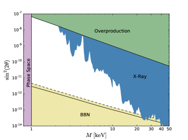
Figure 19: Constraints on mass and mixing for $N_{1}$ making up all of dark matter. The colored regions are excluded. A lepton asymmetry affects the proton-to-neutron ratio during big bang nucleosynthesis (BBN), which gives rise to an upper limit on the lepton asymmetry. The BBN limit given by the solid black line holds if all of the input lepton asymmetry is only in the muon flavor. The dashed line corresponds to the BBN limit if the lepton asymmetry is split equally among all three flavors. Large mixing angles are excluded because too much dark matter would be produced, or because x rays from the decay $N_{1}\to\nu\gamma$ would have already been detected. Additional constraints (not shown) come from structure formation Schneider (2016). From Bodeker and Klaus (2020).

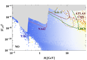
Figure 20: Mixing $U_{\mu i}^{2}$ of heavy neutrinos $N_{i}$ with leptons $l_{\mu}$ as a function of the heavy-neutrino mass $M_{i}$. The gray region is excluded by direct searches of heavy neutral leptons, and the lines show the expected sensitivities for the ongoing T2K, NA62, Belle II, LHCb, ATLAS, and CMS experiments. The parameter f.t. measures the amount of fine-tuning for Yukawa couplings needed for successful leptogenesis. From Abada et al. (2019).

A much studied scenario is an extension of the SM by three sterile neutrinos in which the two heavier ones ($N_{2,3}$) can generate the baryon asymmetry, and the lightest ($N_{1}$) is available as a dark matter candidate (the neutrino minimal standard model). It is noteworthy that such a minimal extension might account for neutrino oscillations, baryogenesis, and dark matter (Asaka, Blanchet, and Shaposhnikov, 2005; Asaka and Shaposhnikov, 2005). The observed baryon asymmetry requires lepton chemical potentials $\mu_{\alpha}/T\sim 10^{-10}$ at $T\sim T_{\rm EW}$. Below $T_{\rm EW}$, the sphaleron processes are ineffective, so a change of the lepton chemical potential no longer affects the baryon asymmetry. Eventually, $N_{2}$ and $N_{3}$ decay and thereby increase the lepton asymmetry. Now large lepton chemical potentials are needed to generate, resonantly amplified, the observed amount of dark matter: $\mu_{\alpha}/T\gtrsim 8\cdot 10^{-6}$ at $T\sim 100~{}\mathrm{MeV}$. The lightest sterile neutrino $N_{1}$ provides dark matter. It has a mass in the range $1<M_{1}\lesssim 50~{}\mathrm{keV}$ and small mixings, $10^{-13}\lesssim\sin^{2}(2\theta_{\alpha 1})\lesssim 10^{-7}$, such that the decay rate is small and it can survive until today. Various constraints are shown in Fig. 19. Moreover, the scenario predicts that the lightest neutrino mass effectively vanishes ($m_{1}\simeq 0$).

Grand unification	GUT-scale leptogenesis
Fermion representations of SM	Connection between $B$ and $L$ in GUTs
Gauge coupling unification (large GUT scale)	Small neutrino masses (GUT-scale seesaw)
Proton decay	Majorana neutrinos
Relations between Yukawa couplings	Relation between $B$ and $L$ asymmetries
Proton decay branching ratios	Neutrino masses and mixings

Table 2: Comparison between qualitative and quantitative aspects of GUTs and leptogenesis, respectively.

This scenario requires a high mass degeneracy of the heavier sterile neutrinos Canetti et al. (2013b, a)

$$|M_{2}-M_{3}|/|M_{2}+M_{3}|\sim 10^{-11}\ .$$ (126)

It is an interesting possibility that the predicted monochromatic x ray line produced by $N_{1}$ dark matter decays corresponds to an unidentified observed x ray line at around $3.5~{}\text{keV}$ Bulbul et al. (2014); Boyarsky et al. (2014). This identification has been challenged by blank-sky observations (Dessert, Rodd, and Safdi, 2020) but is still under discussion Boyarsky et al. (2020).

The extreme fine-tuning of the masses in Eq. (126) is no longer needed if one does not require the generation of lepton asymmetry for the resonant production of $N_{1}$. When processes connecting active and sterile neutrinos with different helicities are taken into account one finds that a 10% splitting is sufficient Antusch et al. (2018).

Models with 3 GeV-scale sterile neutrinos  Drewes and Garbrecht (2013), none of which contribute to the dark matter, have a rich phenomenology. Depending on the parameters, there can be resonant enhancement due to medium effects. In this case only $\mathcal{O}(1)$ tunings for sterile-neutrino masses and mixings are required Abada et al. (2019). Some results of a parameter scan are shown in a mixing-mass plane for sterile neutrinos in Fig. 20, where $U_{\alpha i}\equiv\theta_{\alpha i}=(m_{D}M_{M}^{-1})_{\alpha i}$. There successful leptogenesis is possible with sterile-neutrino masses in the range 0.1–50 GeV. It is encouraging that mixings and masses with successful leptogenesis can be probed through a number of ongoing experiments. Further possibilities to test GeV-scale leptogenesis were discussed by Chun et al. (2018).

IV.5 Leptogenesis: A piece of a puzzle

In its original version leptogenesis was based on a GUT-scale seesaw mechanism with hierarchical heavy Majorana neutrinos. Since their masses are far above collider energies one may wonder whether GUT-scale leptogenesis is at all experimentally testable. In the following we therefore illustrate with a few examples some current hints and conceivable future evidence for leptogenesis at the GUT scale. Both long-baseline neutrino-oscillation experiments and cosmology can be expected to play an important role.

It is instructive to compare possible tests for leptogenesis and GUTs. Hints for grand unification are the fact that quarks and leptons form complete representations of SU(5), the simplest simple group containing the standard model gauge group. Moreover, the gauge couplings of strong and electroweak interactions unify at a large energy scale (GUT scale), approximately without supersymmetry and more precisely with supersymmetry. A generic prediction of GUTs is proton decay. Relations between Yukawa couplings are model dependent. Together with proton decay branching ratios they contain important information about the theory at the GUT scale.

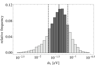
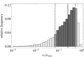
Figure 21: Relative frequency for the leptogenesis parameters $\widetilde{m}_{1}$ (left) and $\varepsilon_{1}$ (right). The solid lines denote the position of the median and the dashed lines are the boundaries of the 68% confidence region. From Buchmuller, Domcke, and Schmitz (2012a).

In a similar way there are qualitative and quantitative hints for GUT-scale leptogenesis: see Table 2. Interactions in GUTs change baryon and lepton number, and the spontaneous breaking of $B\!-\!L$ can generate large Majorana masses for right-handed neutrinos, the basis of leptogenesis. If Yukawa couplings in the neutrino sector are similar to Yukawa coupling for quarks and charged leptons, the seesaw formula (67) automatically yields the right order of magnitude of the neutrino mass scale in terms of the Fermi scale $v_{\text{EW}}\sim 100~{}\text{GeV}$ and the GUT scale $v_{\text{GUT}}\sim 10^{15}~{}\text{GeV}$:

$$m_{3}\sim\frac{v_{\text{EW}}^{2}}{v_{\text{GUT}}}\sim 10^{-2}~{}\text{eV}\ .$$ (127)

A generic prediction of leptogenesis is that light neutrinos are Majorana fermions, which can be probed in neutrinoless double-$\beta$ decay. Moreover, GUTs connect Yukawa matrices in the neutrino sector with those in the charged lepton and quark sectors. Depending on the GUT model, this leads to predictions for neutrino masses and mixings and to relations among the phases that yield the $CP$ violation necessary for leptogenesis.

As an example, consider the following pattern of Dirac neutrino and charged lepton mass matrices that can be obtained in the context of a Froggatt-Nielsen (FN) U(1)-flavour symmetry (Sato and Yanagida, 1998; Irges, Lavignac, and Ramond, 1998):

$$m_{\nu}\sim\frac{v_{\text{EW}}^{2}\sin^{2}\beta}{v_{B-L}}\ \eta^{2a}\ \begin{pmatrix}\eta^{2}&\eta&\eta\\ \eta&1&1\\ \eta&1&1\end{pmatrix}\ ,$$ (128)

$$m_{e}\sim v_{\text{EW}}\cos\beta\ \eta^{a}\begin{pmatrix}\eta^{3}&\eta^{2}&\eta\\ \eta^{2}&\eta&1\\ \eta^{2}&\eta&1\end{pmatrix}\ .$$ (129)

The model has two Higgs doublets, $H_{u}$ and $H_{d}$, which replace $\phi$ and $\tilde{\phi}$ in Eq. (66), respectively, and $v_{\text{EW}}=\sqrt{\langle H_{u}\rangle^{2}+\langle H_{d}\rangle^{2}}$. The vacuum expectation value $v_{B-L}\sim v_{\text{GUT}}$ breaks ${B-L}$, and $\tan\beta=\langle H_{u}\rangle/\langle H_{d}\rangle$. $\eta=1/\sqrt{300}$ is the hierarchy parameter of the FN model, and $a$ and $a+1$ are the FN charges of the $5^{*}$-plets in an SU(5) GUT model Buchmuller and Yanagida (1999). $m_{\nu}$ is determined by the seesaw formula (67), where the FN charges of the right-handed neutrinos drop out. $\mathcal{O}(1)$ factors in the mass matrices remain unspecified in a FN model.

To find out whether a certain pattern of mass matrices can describe the measured data, it is instructive to treat $\mathcal{O}(1)$ parameters as random numbers and to perform a statistical analysis (Hall, Murayama, and Weiner, 2000; Sato and Yanagida, 2000; Vissani, 2001). A detailed study taking the two measured neutrino mass-squared differences and two mixing angles as input was performed by (Buchmuller, Domcke, and Schmitz, 2012a). The parameter scan leads to a prediction for the “most likely” values of the third mixing angle and for phases of the light-neutrino mass matrix. Choosing $\tan\beta\in[1,60]$, with $\sin\beta\in[1/\sqrt{2},1)$, the parameter $a\in[0,1]$ is determined from the normalization of $m_{e}$. The effective $B-L$ breaking scale $\bar{v}_{B-L}=v_{B-L}/\sin^{2}\beta\eta^{2a}$ is determined by the normalization of $m_{\nu}$ and peaks at $\bar{v}_{B-L}=1\times 10^{15}~{}\text{GeV}$, i.e., close to the GUT scale. The most interesting quantities for leptogenesis are the effective light-neutrino mass $\widetilde{m}_{1}$ [see Eq. (105)], the $CP$ asymmetry $\varepsilon_{1}$ [see Eq. (76)], and the absolute neutrino mass scale $\overline{m}$ [see Eq. (105)] or, equivalently, $m_{1}$. The statistical analysis (see Fig. 21) implies normal hierarchy with the neutrino masses

$$m_{1}=2.2^{+1.7}_{-1.4}\times 10^{-3}\ \text{eV},\ \widetilde{m}_{1}=4.0^{+3.1}_{-2.0}\times 10^{-2}\ \text{eV}\ ,$$ (130)

and the $CP$ asymmetry

$$\frac{\varepsilon_{1}}{\varepsilon_{\text{max}}}=0.25^{+0.28}_{-0.18}\ ,$$ (131)

where the maximal $CP$ asymmetry $\varepsilon_{\text{max}}$ is given in Eq. (109). Note that the values for $m_{1}$ and $\widetilde{m}_{1}$ lie inside the neutrino mass window [Eq. (111)]. From Eqs. (104), (108), (130), and (131) one obtains a lower bound on the mass of $N_{1}$ ($M_{1}/\sin^{2}\beta\gtrsim 3\times 10^{11}~{}\text{GeV}$) that is in accord with Fig. 15. Hence, an SU(5) GUT model that successfully describes the light-neutrino masses also naturally explains the observed matter-antimatter asymmetry.

Neutrinoless double-beta decay is sensitive to the effective mass $m_{ee}$, for which one obtains $m_{ee}=1.5^{+0.9}_{-0.8}\times 10^{-3}\,\text{eV}.$ Cosmological observations measure the sum of neutrino masses, which is predicted to be $m_{\text{tot}}=6.0^{+0.3}_{-0.3}\times 10^{-2}\,\text{eV}$. Similar statistical analyses have been carried out by several groups; see Altarelli et al. (2012) and Lu and Murayama (2014). If the condition $\text{det}(m_{\nu})=0$ is imposed on the light-neutrino mass matrix, the statistical analysis is also sensitive on the leptonic Dirac phase $\delta$ (Kaneta, Tanimoto, and Yanagida, 2017).

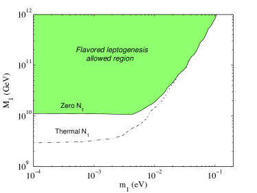
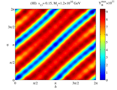
Figure 22: Left panel: region of successful flavored leptogenesis in the ($m_{1}$,$M_{1}$) plane for zero and thermal initial $N_{1}$ abundance. Right panel: correlation between Dirac phase and Majorana phase yielding maximal baryon asymmetry (normal hierarchy). From Branco, Gonzalez Felipe, and Joaquim (2007).

An important ingredient of leptogenesis is the $CP$-violating phases in the neutrino mass matrices Branco et al. (2012a); Hagedorn et al. (2018). Three low-energy phases appear in the light-neutrino mass matrix, the Dirac phase $\delta$ and the two Majorana phases $\alpha$ and $\beta$; see Eq. (70). At present there is evidence for the Dirac neutrino phase $\delta\approx 3\pi/2$ Abe et al. (2020), and the observation of neutrinoless double-beta decay would constrain the Majorana phases $\alpha$ and $\beta$. In the one-flavor approximation, phases beyond the measurable low-energy phases are needed to obtain a nonvanishing $CP$ asymmetry $\varepsilon_{1}$. It is therefore interesting that flavor effects can yield a nonzero $CP$ asymmetry even for vanishing high-energy phases Nardi et al. (2006b); Blanchet and Di Bari (2007); Branco et al. (2007); Pascoli et al. (2007). This effect was studied in the two-flavor regime $10^{9}<M_{1}<10^{12}~{}\text{GeV}$ by Branco, Gonzalez Felipe, and Joaquim (2007) under the assumption that $CP$ violation arises solely from the left-handed neutrino sector. Successful leptogenesis is obtained for $10^{10}<M_{1}<10^{12}~{}\text{GeV}$ and $m_{1}<0.1~{}\text{eV}$ (see Fig. 22, left panel), and a relation between the Dirac phase and one Majorana phase can be read off from the right panel of Fig. 22. In some GUT models leptonic $CP$ violation can indeed be restricted to the left-handed lepton sector. For instance, in the previously described SU(5) model this is achieved by choosing the Yukawa couplings $h^{\nu}$ in the manner described by Branco, Gonzalez Felipe, and Joaquim (2007). Note that this does not affect $CP$ violation in the quark sector.

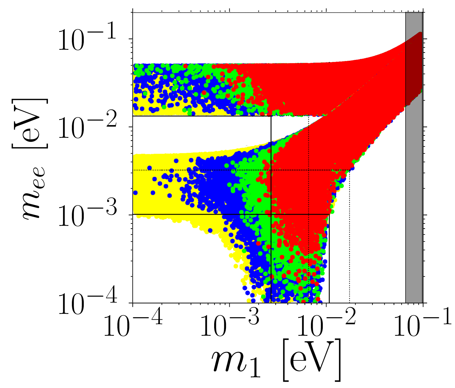
Figure 23: Scatterplot in the ($m_{1}$,$m_{ee}$) plane where the washout of large initial asymmetries is required: $N^{i}_{B-L}=0.1(\text{red}),0.01(\text{green}),0.001(\text{blue})$; the vertical lines indicate the values of $m_{1}$ in the three cases, beyond which 99% of the scatter points are found. From Di Bari, King, and Re Fiorentin (2014).

The absolute neutrino mass scale plays an important role for washout processes. In the one-flavor approximation it was shown that the generated lepton asymmetry becomes rather insensitive to an initial lepton asymmetry of different origin for light-neutrino masses in the strong-washout regime ($m_{i}\gtrsim 10^{-3}~{}\text{eV}$) (Buchmuller, Di Bari, and Plumacher, 2003). However, this lower bound on neutrino masses is sensitive to flavor processes. In a range of parameter space where the asymmetry generation is dominated by $N_{2}$ and washout processes by $N_{1}$, respectively, this was analyzed by Di Bari et al. (2014). Some results of a parameter scan are shown for the ($m_{1}$,$m_{ee}$) plane in Fig. 23. Large initial asymmetries, $N^{i}_{B-L}=0.1(\text{red}),0.01(\text{green}),0.001(\text{blue})$, can be erased for $m_{1}\gtrsim 10~{}\text{meV}$. This has to be compared with cosmological bounds on $m_{\text{tot}}$. A combined analysis of CMB and Lyman-alpha data yields the upper bound $m_{\text{tot}}<0.12~{}\text{eV}$ Palanque-Delabrouille et al. (2015), which is consistent with recent Planck data combined with lensing and baryon acoustic oscillation (BAO) data Aghanim et al. (2020b). A measurement of a total neutrino mass $m_{\text{tot}}\sim 100~{}\text{meV}$ with an uncertainty of $\sim 10~{}\text{meV}$ is challenging, but it would have a strong impact on our understanding of leptogenesis.

The connection between leptogenesis and GUT models has been studied in many explicit models. For examples and references, see Mohapatra and Smirnov (2006) and Altarelli and Feruglio (2010).

IV.6 Toward a theory of leptogenesis

The description of a nonequilibrium process on the basis of thermal field theory, and without any ad hoc assumptions, is a highly nontrivial problem, even for simpler condensed-matter systems. Owing to favorable circumstances that are described later, over the years this goal has essentially been reached for leptogenesis. Hence, this process can be expected to be of general interest in statistical physics, independent of cosmology.

Thermal leptogenesis takes place in an expanding universe with decreasing temperature. Traditionally it has been treated using a set of Boltzmann equations containing $S$-matrix elements that assume scattering in vacuum rather than in a hot plasma. Quantum interference plays a key role in generating the asymmetry, and it is important to understand whether and how this is affected by the presence of the plasma. Furthermore, the role of gauge interactions has long been unclear, and it turned out that their role can be quite important. As in most of Sec. IV.B and IV.C we consider hierarchical heavy neutrinos in the following, and the relevant Yukawa couplings $h^{\nu}$ are therefore small.

Leptogenesis is relatively simple compared to electroweak baryogenesis for the following reasons:

1. It is homogeneous.

2. Few degrees of freedom are involved. Therefore, most degrees of freedom are in thermal equilibrium.

3. The neutrino Yukawa couplings are small. Therefore, there is at least one good set of expansion parameters, which allows for well controlled perturbative approximations.

Given the model, the values of the parameters, and the initial condition, one can then systematically compute the produced asymmetry in a controlled perturbative expansion.

IV.6.1 Effective kinetic equations

In the limit of vanishing neutrino Yukawa couplings $h^{\nu}$ some key quantities, such as $B-L$ and the phase-space density of sterile neutrinos, are covariantly conserved. Since $h^{\nu}$ are small, these quantities change slowly. On the other hand, many SM interactions, the so-called spectator processes, are fast, leading to a hierarchy of timescales. Furthermore, the bulk of the degrees of freedom of the system participates in the spectator processes, giving rise to a well-defined temperature.

The time evolution of the slowly changing quantities is determined by classical equations. When their values are sufficiently close to their equilibrium values the equations are linear. Since the time evolution is slow, only first-time derivatives appear. The coefficients in the equations depend only on the temperature and can be written in terms of real-time correlation functions evaluated at finite temperature, so all medium effects are included. For weak coupling these coefficients can be systematically calculated in perturbation theory.

For an illustration, consider the simple case in which, by the time the baryon asymmetry is produced, the temperature is much smaller than the mass of the lightest sterile neutrino $N\equiv N_{1}$. The sterile neutrinos are then nonrelativistic, and their motion can be neglected. Furthermore, assume that $M_{i}\gg M_{1}$ for the other sterile neutrinos, so that their density can be neglected. Finally, assume that the temperature is so high that none of the charged lepton Yukawa interactions are fast. The only slow quantities are then the density of the lightest sterile neutrino $n_{N}$ and $B-L$, and the nonequilibrium system is described by the following effective kinetic equations Bodeker and Wörmann (2014)

$$\dot{n}_{N}+3Hn_{N}\,\,\,= {}-\Gamma_{N}\,\,(n_{N}-n_{N}^{\rm eq})$$

$$\,+\Gamma_{N,B-L}\,n_{B-L},$$ (132)

$$\dot{n}_{B-L}+3Hn_{B-L}= \,\,\Gamma_{B-L,N}(n_{N}-n_{N}^{\rm eq})$$

$$-\Gamma_{B-L}\,n_{B-L},$$ (133)

while the rest of the degrees of freedom is determined by the temperature $T$. The coefficients $\Gamma_{i}$ depend only on $T$. Note that Eqs. (132) and (133) have the same form as Eqs. (90) and  (99). However, to arrive at Eqs. (132) and (133), no Boltzmann equation or $S$ matrix was used: the only ingredient was the separation of timescales. Correspondingly, Eqs. (132) and (133) are valid to all orders in the SM coupling, and the coefficients include the effect of all possible processes.

When describing the simplest possible case, Eqs. (132) and (133) already display the general structure of all kinetic equations describing leptogenesis. In general, the sterile neutrinos must be described by phase-space densities, depending not only on time but also on momentum. This is because relativistic effects can be important, and because the rates that change the momenta of sterile neutrinos are parametrically of the same size as for the change of number densities, so that one cannot always assume kinetic equilibrium. Another generalization is that the densities turn into flavor-space matrices of densities, and that the spin of the sterile neutrinos has to be accounted for as well.

The rate coefficients can be computed as follows. Even in thermal equilibrium, physical quantities fluctuate around their equilibrium values, and the fluctuations of slowly varying variables are described by the same kinetic equations as the deviations from equilibrium. Therefore one can compute unequal time correlation functions of slow variables using the effective kinetic equations. By matching the result to the same correlation function computed in quantum field theory at frequencies $\Gamma_{i}\ll\omega\ll\omega_{\rm spec}$ one can relate $\Gamma_{i}$ to correlation functions of SM operators evaluated at finite temperature Bodeker and Laine (2014). The most important correlation function that one encounters is the two-point spectral function of the operator to which the sterile neutrinos couple [see Eq. (66)]

$$\widetilde{\rho}_{i}(p)\,\equiv\frac{1}{3}\int\!{\rm d}^{4}x\,e^{ip\cdot x}\Bigl{\langle}\,\Bigl{\{}(\phi^{\dagger}l_{i})(x),(\overline{l\,}_{\!i}\,\phi)(0)\Bigr{\}}\,\Bigr{\rangle},$$ (134)

where the expectation value is taken in an equilibrium ensemble of standard model fields only. For example, the $\Delta L=1$ washout rate in the one-flavor regime can be written as  Bodeker and Laine (2014)

$$\Gamma_{B-L}=|h^{\nu}|^{2}{\cal W}\Xi^{-1},$$ (135)

with

$${\cal W}=-\int\frac{d^{3}p}{(2\pi)^{3}}\frac{f_{\rm F}^{\prime}(E_{1})}{2E_{1}}{\rm tr}\Big{\{}\not{p}\big{[}\widetilde{\rho}(p)+\widetilde{\rho}(-p)\big{]}\Big{\}},$$ (136)

where ${p^{0}=E_{1}}$. Furthermore,

$$\Xi\equiv\frac{1}{TV}\left\langle(B-L)^{2}\right\rangle$$ (137)

is the $B-L$ susceptibility. Its value depends on which reactions are fast, i.e., which spectator processes are active. At high temperatures ($T\gg 10^{13}~{}\text{GeV}$), where only SM gauge interactions and the top-Yukawa interactions are fast, the leading-order susceptibility is $\Xi=T^{2}/4$. Equation (135) illustrates the general structure of the rates that consist of a spectral function, which is a real-time-dependent quantity, and an inverse susceptibility, which is determined using equilibrium thermodynamics. It can be compared to Eq. (100). When SM interactions are neglected, $\cal W$ is proportional to the rate $\gamma_{N}$. Furthermore, $\Xi$ is then proportional to $\int d^{3}pf_{F}(1-f_{F})$ where $f_{F}$ is the Fermi distribution function. If we approximate this using Boltzmann statistics, $\Xi$ is proportional to $n_{l}^{\rm eq}$.

The rate $\Gamma_{N}$ in Eq. (132) contains the same spectral function as $\Gamma_{B-L}$ (Laine and Schroder, 2012; Bodeker, Sangel, and Wörmann, 2016). In fact, for leptogenesis through sterile-neutrino oscillations all coefficients in the kinetic equations can be written in terms of the spectral function in Eq. (134) Ghiglieri and Laine (2017); Bodeker and Schröder (2020).

When computing the rates $\Gamma_{i}$ in perturbation theory, one has to distinguish among several temperature regimes. The nonrelativistic case $T\ll M_{1}$ is relevant mostly for thermal leptogenesis in the strong-washout regime, while leptogenesis through oscillations proceeds entirely in the ultrarelativistic regime $T\mbox{~{}{\raisebox{1.72218pt}{$>$}} {\raisebox{-2.58334pt}{$\sim$}}~{}}M_{1}/g$, where $g$ denotes a combination of electroweak gauge and top-Yukawa coupling.

When $T\mbox{~{}{\raisebox{1.72218pt}{$<$}} {\raisebox{-2.58334pt}{$\sim$}}~{}}M_{1}$, at leading order in the couplings the rates are determined by decays and inverse decays. In addition to these $\Delta L=1$ processes, for the washout rate $\Gamma_{B-L}$ one has to take into account the $\Delta L=2$ processes, even though these are ${\cal O}(h^{\nu})^{4}$ and thus appear to be highly suppressed. Nevertheless, they play a crucial role at late times when $T\ll M_{N_{1}}$: The $\Delta L=1$ rates are then Boltzmann suppressed with $\exp(-M_{N}/T)$, while the $\Delta L=2$ rates are only power suppressed, so they eventually dominate at low $T$, which causes the kink of $\Gamma_{W}$ in Fig. 14 (top panel). Since it plays a role only at $T\ll M_{1}$, it can be obtained by integrating out the sterile neutrinos. Instead of from Eq. (135) it follows from the two-point function of the Weinberg operator containing two Higgs and two lepton fields in Eq. (74) (Sangel, 2016).

For $T\mbox{~{}{\raisebox{1.72218pt}{$>$}} {\raisebox{-2.58334pt}{$\sim$}}~{}}M_{1}$ Eq. (132) is replaced by an equation for the phase-space density with a momentum-dependent $\Gamma_{N}$ :

$$\dot{f}_{N}+3H{\bf p}\cdot\frac{\partial f_{N}}{\partial{\bf p}}\,\,\, ={}-\Gamma_{N}({\bf p})\left(f_{N}-f_{N}^{\rm eq}\right)+\cdots.$$ (138)

On the other hand, the asymmetry is still described by a space density because it is carried by SM particles that are kept in kinetic equilibrium by the fast gauge interactions:

$$\dot{n}_{B-L}+3Hn_{B-L}=\int\!\!\frac{d^{3}p}{(2\pi)^{3}}\Gamma_{B-L,N}({\bf p})\left(f_{N}-f_{N}^{\rm eq}\right)+\cdots.$$ (139)

In the ultrarelativistic regime plasma effects have a profound influence on the rates, and gauge interactions are dominant. While at $T\mbox{~{}{\raisebox{1.72218pt}{$<$}} {\raisebox{-2.58334pt}{$\sim$}}~{}}M_{1}$ the $2\to 2$ scatterings are higher order, the inverse decays are phase space suppressed when $T\gg M_{1}$. Without taking into account thermal masses, the $2\to 2$ scatterings would be dominant, as can be seen in Fig. 14 (top panel). However, when the thermal masses of the SM particles are included, both types of processes contribute at leading order. The resulting production rate at vanishing density $(dn_{N}/dt)_{n_{N}=0}=2(2\pi)^{-3}\int d^{3}p\Gamma_{N}({\bf p})f_{N}^{\rm eq}$ is shown in Fig. 24 (dotted line). At high temperatures the rate is due to Higgs decays that are made possible by the large thermal Higgs mass. For a small sterile-neutrino mass this could be the main source of the baryon asymmetry Hambye and Teresi (2016). Additional multiple interactions mediated by soft gauge bosons turn out to be of crucial importance and have to be resummed [Landau-Pomeranchuk-Migdal (LPM) resummation; see Fig. 25], giving rise to the full curve in Fig. 24 (Anisimov, Besak, and Bodeker, 2011b). The same results in the limit $T\gg M_{1}$ are shown in Fig. 26, together with the $2\to 2$ scattering rates. The LPM-resummed inverse decays and the $2\to 2$ scattering rates give similar contributions, with the latter dominating at higher temperatures. The contributions involving gauge bosons increase the total rate by almost an order of magnitude compared to the top-quark scattering shown in Fig. 14.

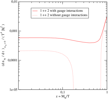
Figure 24: Number of produced Majorana neutrinos per unit time and unit volume as a function of the temperature for $M_{N}=10^{7}$ GeV. The dotted curve is the result with thermal masses included but without any soft gauge interactions. The full line includes an arbitray number of soft gauge interactions, as illustrated in Fig. 25. From Anisimov, Besak, and Bodeker (2011b).

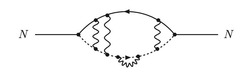
Figure 25: Self-energy diagram with soft gauge bosons for Majorana neutrino $N$, whose imaginary part contributes to leading order to the $N$-production rate. From Anisimov, Besak, and Bodeker (2011b).

Figure 26: Number of produced massless Majorana neutrinos per unit time and unit volume as a function of the temperature. All leading-order contributions are shown. $1\leftrightarrow 2$ are the inverse decay processes without and with multiple scattering mediated by soft gauge bosons displayed in Fig. 24. The $2\to 2$ scattering contributions involving gauge bosons are of similar size and dominate at high $T$, while the top-quark scattering is always subdominant. From Anisimov et al. (2011b).

Since all rates for leptogenesis can be written in terms of finite-temperature correlation functions, one can systematically compute higher orders of SM corrections, of which there are two types. The first are corrections to the susceptibilities, which are related to the chemical potentials and the asymmetry densities. These are relatively simple to compute because they are thermodynamic quantities involving no time dependence. The corrections to the susceptibilities already start at the order of $g$, and are less than 30% Bodeker and Laine (2014); Bodeker and Sangel (2015). The occurrence of odd powers of the coupling is typical for infrared effects in thermal field theory, and in this case they are due to soft Higgs exchange. The second type are corrections to spectral functions as in Eq. (134) that are of the order of $g^{2}$. These are more difficult to compute since they are real-time correlation functions. For the nonrelativistic limit where Eqs. (132) and (133) hold, all rates have been computed at order $g^{2}$ in a high-temperature expansion, i.e., $\Gamma_{N}$ (Salvio, Lodone, and Strumia, 2011; Laine and Schroder, 2012) and the washout rate Bodeker and Laine (2014). The most interesting one $\Gamma_{B-L,N}$, which is responsible for the asymmetry, is also the most difficult to calculate. It is related to the three-point function of the operators appearing in Eq. (134) Bodeker and Sangel (2017) rather than the two-point function. In the region where the high-temperature expansion is applicable, the corrections are a few percent. The next-to-leading-order (NLO) production rate was computed in the relativistic regime $T\sim M_{1}$ by Laine (2013), and to the washout rate by Bodeker and Laine (2014); see Fig. 27.

Figure 27: Function $\mathcal{W}$ appearing in the washout rate in Eq. (135). Shown are the LO result including thermal masses (dotted line), the relativistic NLO result, and the NLO result in the nonrelativistic approximation (dashed line). Also shown is the LO LPM-resummed result that is valid in the ultrarelativistic regime ($M_{I}\mbox{~{}{\raisebox{1.72218pt}{$<$}} {\raisebox{-2.58334pt}{$\sim$}}~{}}gT$) (dash-dotted line). From Bodeker and Laine (2014).

In the strong-washout regime [see Eq. (106)] the relativistic corrections and the radiative corrections to $\Gamma_{N}$ affect the produced baryon asymmetry at the level of a few percent  Bodeker and Wörmann (2014). The corrections to the $\Delta L=1$ washout rate $\Gamma_{B-L}$, to the asymmetry rate $\Gamma_{B-L,N}$, and to the $\Delta L=2$ washout rate (Sangel, 2016) were not included in this analysis, but they are of similar size as the corrections to $\Gamma_{N}$ and are not expected to lead to larger corrections to the produced asymmetry.

IV.6.2 Kadanoff-Baym equations

Leptogenesis involves quantum interferences in a crucial manner, so the standard approach by means of classical Boltzmann equations may appear problematic. Using the Schwinger-Keldysh, or closed-time-path, formalism Schwinger (1961); Keldysh (1964), a full quantum field-theoretical treatment of leptogenesis can be based on Green’s functions Buchmuller and Fredenhagen (2000). In the Schwinger-Keldysh formalism one considers Green’s functions $\Delta$ on a complex time contour starting at some initial time $t_{i}$; see Fig. 28. They satisfy the following Schwinger-Dyson equations with self-energies $\Pi_{C}$:

$$( \Box_{1}+m^{2})\Delta_{C}(x_{1},x_{2})$$ (140)

$$+\int_{C}d^{4}x^{\prime}\Pi_{C}(x_{1},x^{\prime})\Delta_{C}(x^{\prime},x_{2})=-i\delta_{C}(x_{1}-x_{2}).$$

It is convenient to consider two correlation functions, the spectral functions $\Delta^{-}$, which contain information about the system, and the statistical propagators $\Delta^{+}$, which depend on the initial state at time $t_{i}$:

$$\begin{split}\Delta^{+}(x_{1},x_{2})&=\tfrac{1}{2}\langle\{\Phi(x_{1}),\Phi(x_{2})\}\rangle\ ,\\ \Delta^{-}(x_{1},x_{2})&=i\langle[\Phi(x_{1}),\Phi(x_{2})]\rangle\ .\end{split}$$ (141)

Figure 28: Path in the complex time plane for nonequilibrium Green’s functions.

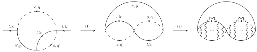
Figure 29: Transformation of the lepton self-energy diagram to a “double-blob” diagram amenable to resummation. From Depta et al. (2020).

These correlation functions satisfy the following Kadanoff-Baym equations Baym and Kadanoff (1961); Berges (2004):

$$\begin{split}\Box_{1,{\bf q}}\Delta^{-}_{\bf q}(t_{1},t_{2})=&-\int_{t_{2}}^{t_{1}}dt^{\prime}\Pi^{-}_{\bf q}(t_{1},t^{\prime})\Delta^{-}_{\bf q}(t^{\prime},t_{2})\ ,\\ \Box_{1,{\bf q}}\Delta^{+}_{\bf q}(t_{1},t_{2})=&-\int_{t_{i}}^{t_{1}}dt^{\prime}\Pi^{-}_{\bf q}(t_{1},t^{\prime})\Delta^{+}_{\bf q}(t^{\prime},t_{2})\\ &+\int_{t_{i}}^{t_{2}}dt^{\prime}\Pi^{+}_{\bf q}(t_{1},t^{\prime})\Delta^{-}_{\bf q}(t^{\prime},t_{2})\ ,\end{split}$$ (142)

where we have assumed spatial homogeneity and $\Box_{1,{\bf q}}=(\partial^{2}_{t_{1}}+m^{2}+{\bf q}^{2})$ is the d’Alembert operator for a momentum mode ${\bf q}$.

For leptogenesis one has to consider two Green’s functions: $S^{\pm}_{Lij}(x,x^{\prime})$ for the lepton doublets, where $i$ and $j$ denote lepton flavors, and $G^{\pm}(x,x^{\prime})$ for the heavy Majorana neutrino. The lepton current is given by

$$j^{\mu}_{ij}(x)=-\text{tr}[\gamma^{\mu}S^{+}_{Lij}(x,x)]|_{x^{\prime}\rightarrow x}\ .$$ (143)

The nonequilibrium leptogenesis process is a transition from some initial state to a final state with nonzero chemical potential in thermal equilibrium. To compare results from Boltzmann equations and Kadanoff-Baym equations, a simplified case was considered by Anisimov et al. (2010), who focused on the $CP$-violating source term for the asymmetry and ignored washout terms and Hubble expansion. This corresponds to evaluating the initial lepton asymmetry, generated until the heavy neutrino reaches thermal equilibrium, starting from zero initial abundance. Since we consider a spatially homogeneous system, it is convenient to perform a Fourier expansion. For a momentum mode $\bf k$ diagonal elements of the charge density matrix can be interpreted as differences of phase-space distribution functions for leptons and antileptons:

$$\begin{split}L_{{\bf k}ii}(t,t)&=-\text{tr}[\gamma_{0}S^{+}_{L{\bf k}ij}(t,t)]\\ &=f_{li}(t,k)-f_{\bar{l}i}(t,k)\ .\end{split}$$ (144)

Note that, contrary to a system in thermal equilibrium, the distribution functions are time dependent.

The calculation of the asymmetry starts from a Green’s function for the heavy neutrino that interpolates between a free Green’s function and an equilibrium Green’s function Anisimov et al. (2009). The lepton asymmetry is then obtained from the two-loop diagram (Anisimov et al., 2011) in the left panel of Fig. 29. In this calculation the effect of soft gauge-boson exchange turns out to be of crucial importance. For the production of heavy neutrinos they were already included by Anisimov et al. (2011a); see Figs. 25 and 24. For the $CP$ asymmetry their effect was estimated by introducing phenomenological thermal widths by Anisimov et al. (2011a). Recently the summation over soft gauge bosons was also completed for the $CP$ asymmetry Depta et al. (2020). The strategy for calculating the lepton asymmetry is illustrated in Fig. 29. Integrating over lepton momenta corresponds to closing the external lepton line, and summation of the gauge-boson interactions leads to the double-blob diagram. The corresponding expression for the lepton asymmetry has been evaluated using a combination of analytical and numerical techniques. The result takes the form

$$\begin{split}n_{L,ii}(t)&=\int\frac{d^{3}k}{(2\pi)^{3}}L_{{\bf k}ii}(t,t)\\ &\simeq-\varepsilon_{ii}F(T)\frac{1}{\Gamma_{N}}\left(1-e^{-\Gamma_{N}t}\right)\ ,\end{split}$$ (145)

where the momentum dependence of the thermal $N$-decay width has been neglected and $F(T)$ is given as a complicated momentum integral. The results for Boltzmann equations and Kadanoff-Baym equations with thermal widths have the same form, with different functions $F(T)$ Anisimov et al. (2011a).

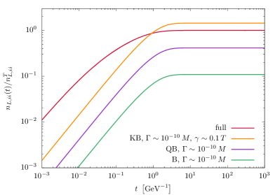
Figure 30: Comparison of the Kadanoff-Baym computation including LPM-resummed gauge interactions (full), without computing gauge interactions but instead parametrizing them with thermal widths (KB), with Boltzmann equation containing (inverse) sterile-neutrino decays using classical statistics (B) and quantum statistics (QB). The mass of the lightest heavy neutrino is $10^{10}$ GeV, the temperature is constant at $10^{11}$ GeV. This corresponds to the previously discussed ultrarelativistic regime $T\mbox{~{}{\raisebox{1.72218pt}{$>$}} {\raisebox{-2.58334pt}{$\sim$}}~{}}M/g$ . From Depta et al. (2020).

The generated asymmetries are compared in Fig. 30 for the different cases. For $t<\Gamma_{N}^{-1}\sim 1~{}\text{GeV}^{-1}$, there is a difference in shape with respect to the numerical solution for the full Kadanoff-Baym equations. This is a consequence of the approximation $\Gamma_{N}({\bf p})\simeq\Gamma_{N}$. The generated final lepton asymmetries differ by factors of $\mathcal{O}(1)$.

At first sight, the simple time dependence of the asymmetry (145) may appear to be surprising. However, it is easily understood as a consequence of the effective kinetic equations (132) and (133) for distribution functions. For constant temperature, the equation for $n_{N}$ has the solution $n_{N}(t)\simeq n_{N}^{\text{eq}}[1-\exp(-\Gamma_{N}t)]$ Anisimov et al. (2010) and, if we neglect washout effects, the solution for $n_{B-L}$ simply inherits this time dependence. Viewed in this way, solving the Kadanoff-Baym equations appears to be a way to calculate coefficients in effective kinetic equations.

The Kadanoff-Baym equations have also been used to obtain effective equations of motion. This way corrections to the $CP$-violating parameter were obtained Garny et al. (2009, 2010) and the leading-order asymmetry rate in the relativistic regime $T\sim M_{1}$ was computed Beneke et al. (2010). When lepton Yukawa interaction rates are of a similar size as the Hubble parameter, these also have to be included in the network of kinetic equations, and the lepton asymmetries are described by matrices in flavor space that can account for the unflavored as well as the fully flavored regime Beneke et al. (2011). The case of resonant leptogenesis was considered by De Simone and Riotto (2007) and an approximate analytical solution was given by Garny, Kartavtsev, and Hohenegger (2013). Leptogenesis through oscillations (Sec. IV.4) was treated by Drewes and Garbrecht (2013).

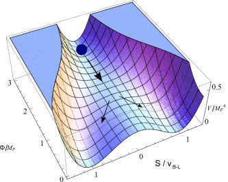
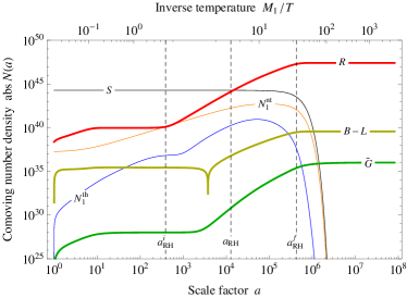
Figure 31: Left panel: hybrid inflation. The time evolution of the inflaton field $\Phi$ leads to a tachyonic mass of the waterfall field $S$ that triggers a rapid transition to a phase with spontaneously broken $B-L$ symmetry. Right panel: comoving number densities of the particles of the $B-L$ Higgs sector ($S$), the thermal and nonthermal (s)neutrinos $(N_{1}^{\text{th}},N_{1}^{\text{nt}})$, the MSSM radiation ($R$), the gravitinos $(\tilde{G})$, and the $B-L$ asymmetry. Values were obtained by solving the Boltzmann equations for $v_{B-L}=5\times 10^{15}~{}\text{GeV}$, $M_{1}=5.4\times 10^{10}~{}\text{GeV}$, and $\widetilde{m}_{1}=4.0\times 10^{-2}~{}\text{eV}$. From Buchmuller et al. (2013a).

IV.7 Leptogenesis, inflation, and gravitational waves

Some evidence for GUT-scale leptogenesis may be obtained via the constraints that GUTs impose on neutrino masses and mixings and that influence the size of the lepton asymmetry. Similarly, leptogenesis is part of the early cosmological evolution and thereby related to the other two main puzzles in cosmology, dark matter and inflation. To work out these connections quantitatively is important for obtaining a coherent and convincing picture of the early universe.

In this respect it is interesting that, complementary to thermal leptogenesis, nonthermal leptogenesis can be responsible for the baryon asymmetry of the Universe. Here the thermal production of heavy neutrinos is replaced by some nonthermal production, such as inflaton decays Lazarides and Shafi (1991); Asaka et al. (1999, 2000); Hahn-Woernle and Plumacher (2009). In supersymmetric theories the reheating temperature is bounded from above by the requirement to avoid overproduction of gravitinos. If the gravitino is the lightest superparticle (LSP), it can be stable and can form dark matter. Otherwise, LSP dark matter can be produced in gravitino decays (Gherghetta, Giudice, and Wells, 1999).

An interesting possibility is that GUT-scale leptogenesis might be probed by gravitational waves GWs. GWs from inflation can have a characteristic kink in their spectrum indicating the change from an early matter dominated phase to the radiation dominated phase and in this way allow for a measurement of the reheating temperature Nakayama et al. (2008b, a) that is related to the energy scale of nonthermal leptogenesis. In general, however, the GW signal from inflation is too small to be observed anytime soon. In the following we describe another possibility, GWs from cosmic strings produced in a $\text{U(1)}_{B-L}$ phase transition after inflation Buchmuller et al. (2013b). In supersymmetric models leptogenesis is naturally linked to $F$-term hybrid inflation Copeland et al. (1994); Dvali et al. (1994) if one demands spontaneous breaking of $B-L$. The amplitude of the CMB power spectrum then requires the $B-L$ breaking scale to be of the order of the GUT scale. This leads to a large stochastic gravitational wave background that can be probed by ground-based interferometers.

A cosmic-string network can form after the spontaneous breaking of a U(1) symmetry Hindmarsh (2011), and the resulting GW spectrum has been evaluated for Abelian Higgs strings Figueroa et al. (2013, 2020) as well as Nambu Goto strings Damour and Vilenkin (2001); Siemens et al. (2007); Kuroyanagi et al. (2012). If the product of this U(1) group and the SM gauge group results from the spontaneous breaking of a GUT group, the theory contains magnetic monopoles in addition to strings Vilenkin (1982); Martin and Vilenkin (1996); Leblond et al. (2009), and the string network becomes unstable. Recently it was pointed out that GWs from a metastable network of cosmic strings are a generic prediction of the seesaw mechanism Dror et al. (2020). Moreover, it has been shown that, for $\text{U(1)}_{B-L}$ breaking combined with hybrid inflation, a GW signal is predicted that evades the bounds from pulsar timing array (PTA) experiments but will be probed by ongoing and future observations of LIGO-Virgo and KAGRA Buchmuller et al. (2020).

The decay of a false vacuum of unbroken $B-L$ is a natural mechanism to generate the initial conditions of the hot early Universe (Buchmuller, Domcke, and Schmitz, 2012c). The false-vacuum phase yields hybrid inflation and ends in tachyonic preheating Felder et al. (2001); see Fig. 31, left panel. After tachyonic preheating the evolution can be described using a system of Boltzmann equations. Decays of the $B-L$ breaking Higgs field and thermal processes produce an abundance of heavy (s)neutrinos whose decays generate the entropy of the hot early Universe, the baryon asymmetry via leptogenesis, and dark matter in the form of the lightest superparticle Ellis et al. (1984); see Fig. 31 (right panel).

We now consider an extension of the supersymmetric standard model (MSSM) with three right-handed neutrinos that realizes spontaneous $\text{U(1)}_{B-L}$ breaking in the simplest possible way by using three SM-singlet chiral superfields $\Phi$, $S_{1}$, and $S_{2}$:

$$\begin{split}W=&W_{\rm MSSM}+h_{ij}^{\nu}\mathbf{5}_{i}^{*}n_{j}^{c}H_{u}+\frac{1}{\sqrt{2}}\,h_{i}^{n}n_{i}^{c}n_{i}^{c}S_{1}\\ &+\lambda\,\Phi\left(\frac{v_{B-L}^{2}}{2}-S_{1}S_{2}\right)+W_{0}\ .\end{split}$$ (146)

In unitary gauge, $S_{1,2}=S/\sqrt{2}$ corresponds to the physical $B-L$ Higgs field, $\Phi$ plays the role of the inflaton, and the constant $W_{0}$ is tuned to obtain vanishing vacuum energy; $n^{c}_{i}$ contain the charge conjugates of the right-handed neutrinos, the SM leptons belong to the SU(5) multiplets $\mathbf{5}^{*}=(d^{c},\ell)$ and $\mathbf{10}=(q,u^{c},e^{c})$, and the two Higgs doublets are part of the $\mathbf{5}$- and $\mathbf{5^{*}}$-plets $H_{u}$ and $H_{d}$, respectively. Quark and lepton Yukawa couplings are described in the usual way by $W_{\rm MSSM}$. The flavor structure is chosen according to Buchmuller and Yanagida (1999) and was already described in Sec. IV.5.

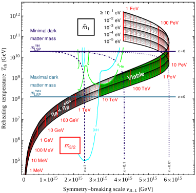
Figure 32: Viable parameter space (green) for hybrid inflation, leptogenesis, neutralino DM, and big bang nucleosynthesis. Hybrid inflation and the dynamics of reheating correlate the parameters $v_{B-L}$, $T_{\text{rh}}$, $m_{3/2}$ and $\widetilde{m}_{1}$ (black curves). Successful leptogenesis occurs outside the gray-shaded region. Neutralino DM is viable in the green region, corresponding to a Higgsino (wino) with mass $100\leq m_{\rm LSP}/\textrm{GeV}\leq 1060$ (2680). From Buchmuller et al. (2020).

The $B-L$ breaking part of $W$ is precisely the superpotential of $F$-term hybrid inflation (FHI). It was widely believed that FHI could not account for the correct scalar spectral index of the CMB power spectrum but the analyses given by Bastero-Gil, King, and Shafi (2007), Nakayama, Takahashi, and Yanagida (2010), Rehman, Shafi, and Wickman (2010), and Buchmuller et al. (2014) showed that FHI is viable once the effect of supersymmetry (SUSY) breaking on the inflaton potential is taken into account. The parameter range consistent with leptogenesis, inflation, and neutralino dark matter (DM), produced in gravitino decays, was analyzed by Buchmuller et al. (2020). The result is shown in Fig. 32. For given values of $\widetilde{m}_{1}$ and the gravitino mass $m_{3/2}$, successful hybrid inflation selects a point in the $v_{B-L}$-$T_{\text{rh}}$ plane. The gray shading in Fig. 32 indicates the region where leptogenesis falls short of explaining the observed baryon asymmetry. Gravitino masses of $\mathcal{O}\left(1\right)\,\textrm{TeV}$ or larger point to a neutralino LSP that is produced thermally as well as nonthermally in gravitino decays (Buchmuller, Domcke, and Schmitz, 2012b). Gravitinos are in turn generated in decays of the $B-L$ Higgs field as well as from the thermal bath; for a discussion and references, see Jeong and Takahashi (2013). Taking into account the fact that gravitinos must decay early enough to preserve big bang nucleosynthesis Kawasaki et al. (2018), as well as the LEP bound on charginos $m_{\text{LSP}}\gtrsim 100$ GeV Tanabashi et al. (2018), a Higgsino or wino LSP can account for the observed DM relic density in the green-shaded region of Fig. 32. It is highly nontrivial that neutralino DM and leptogenesis can be successfully realized in the same parameter region. In summary, the viable parameter region of the described model is given by $v_{B-L}\simeq(3.0$ – $5.8)\times 10^{15}\,\textrm{GeV}$ and $m_{3/2}\simeq 10\,\textrm{TeV}$ – $10\,\textrm{PeV}$.

The considered flavor model corresponds to an embedding of ${G}_{\rm SM}\times\text{U(1)}_{B-L}$ in the gauge group $\text{SU(5)}\times\text{U(1)}_{B-L}$ with the final unbroken group ${G}_{\rm SM}\times\mathbb{Z}_{2}$. This leads to the production of stable cosmic strings in the $\text{U(1)}_{B-L}$ phase transition Dror et al. (2020). However, the model can also be embedded in SO(10) Asaka (2003). In this case, the final unbroken group is ${G}_{\rm SM}$, and there can be no stable strings Dror et al. (2020). Cosmic strings can then decay via the Schwinger production of monopole-antimonopole pairs, leading to a metastable cosmic-string network. The decay rate per string unit length is given by (Monin and Voloshin, 2008, 2010; Leblond, Shlaer, and Siemens, 2009)

$$\Gamma_{d}=\frac{\mu}{2\pi}\exp\left(-\pi\kappa\right)\,,$$ (147)

with $\kappa=m^{2}/\mu$ denoting the ratio between the monopole mass $m\sim v_{\text{GUT}}$ and the cosmic-string tension $\mu\sim v_{B-L}^{2}$. For appropriate values of $v_{B-L}<v_{\rm GUT}$, the cosmic strings are sufficiently long lived to give interesting signatures but decay before emitting low-frequency GWs that are strongly constrained by PTA experiments.

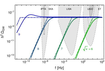
Figure 33: GW spectrum for $G\mu=2\times 10^{-7}$. Different values of $\sqrt{\kappa}$ are indicated in different colors; the blue curve corresponds to a cosmic-string network surviving until today. The dot-dashed lines depict an analytical estimate. The (lighter) gray-shaded areas indicate the sensitivities of (planned) experiments SKA Smits et al. (2009), LISA Amaro-Seoane et al. (2017), LIGO Abbott et al. (2019) and ET Maggiore et al. (2020), the crosses within the SKA band indicate constraints by the IPTA Verbiest et al. (2016). From Buchmuller et al. (2020).

The network of cosmic strings formed during the $B-L$ phase transition acts as a source of GWs. Modeling the evolution and GW emission of a cosmic-string network is a challenging task, resulting in several competing models in the literature; see Auclair et al. (2020) and references therein for a comprehensive review. Moreover, for metastable strings, the GW production from fast-moving monopoles requires further investigation (Vilenkin, 1982; Leblond, Shlaer, and Siemens, 2009). The analysis of Buchmuller et al. (2020) was based on the model of Blanco-Pillado, Olum, and Shlaer (2014), and for the first time the GW spectrum has been calculated for a metastable string network. The GW spectrum reads

$$\Omega_{\text{GW}}(f)=\partial\rho_{\text{GW}}(f)/\rho_{c}\partial\ln{f}\ ,$$ (148)

where $\rho_{\text{GW}}$ and $\rho_{c}$ are GW energy density and critical energy density, respectively. The spectrum is characterized by the following plateau Auclair et al. (2020):

$$\Omega_{\text{GW}}^{\text{plateau}}\simeq 8.04\,\Omega_{r}\left(\frac{G\mu}{\Gamma}\right)^{1/2}\ ,$$ (149)

where $\Gamma\simeq 50$ parametrizes the cosmic-string decay rate into GWs and $\Omega_{r}$ is the energy density in radiation relative to the critical energy density. The GW spectrum has a turnover point at the frequency

$$f_{*}\simeq 3.0\times 10^{14}\,\text{Hz}\>e^{-\pi\kappa/4}\left(\frac{10^{-7}}{G\mu}\right)^{1/2}\ .$$ (150)

Figure 33 shows the GW spectrum obtained by a numerical evaluation as well as the analytical estimate

$$\Omega_{\text{GW}}(f)=\Omega_{\text{GW}}^{\text{plateau}}\;\text{min}\left[(f/f_{*})^{3/2},1\right]\,.$$ (151)

The shaded regions indicate the power-law-integrated sensitivity curves of current and planned experiments Thrane and Romano (2013). For $G\mu=2\times 10^{-7}$, the constraint from the European Pulsar Timing Array Shannon et al. (2015) enforces $\sqrt{\kappa}\lesssim 8$. In the case of a mild hierarchy between the GUT and $B-L$ scales ($m/v_{B-L}\gtrsim 6$), primordial GWs will be probed by LIGO-Virgo Abbott et al. (2019) and KAGRA Akutsu et al. (2019) in the near future.

The general framework behind the described model (inflation ending in a GUT-scale phase transition in combination with leptogenesis and dark matter in a SUSY extension of the SM) provides a testable framework for the physics of the early Universe. A characteristic feature of this framework is a stochastic background of gravitational waves emitted by metastable cosmic strings.

Probing leptogenesis with gravitational waves is an interesting possibility and theoretical work on this subject is just beginning. For recent work, see Blasi, Brdar, and Schmitz (2020) and King et al. (2020).

IV.8 Summary: Leptogenesis

Thermal leptogenesis is now well understood. It is closely related to neutrino masses, and simple estimates, based on GUT models, yield the right order of magnitude for the observed matter-antimatter asymmetry. In the one-flavor approximation successful leptogenesis leads to a preferred mass window for the light neutrinos that is consistent with the cosmological upper bound on the sum of neutrino masses, and to a lower bound on the heavy Majorana neutrino masses. Taking flavor effects into account, the qualitative picture remains valid, but quantitatively the neutrino mass bounds are relaxed. For quasidegenerate heavy neutrinos the temperature scale of leptogenesis can be lowered to the weak scale. $CP$-violating oscillations of sterile neutrinos can lead to successful leptogenesis even for GeV neutrino masses.

Significant progress has been made toward a full description of leptogenesis on the basis of thermal field theory. This has been possible because leptogenesis is a homogeneous process that involves only a few dynamical degrees of freedom with small couplings to a large thermal bath. Effective kinetic equations have been derived, which take the form of ordinary Boltzmann equations whose kernels can be systematically calculated in terms of spectral functions of SM correlation functions. Relativistic and off-shell effects are included in Kadanoff-Baym equations that have also been used to calculate the generated lepton asymmetry. In the field-theoretical treatment, interactions with gauge bosons of the thermal bath turn out to be crucial and have to be resummed. Using these techniques, for the first time an estimate of the theoretical error of traditional calculations based on Boltzmann equations has been obtained; it turns out to be about $50\%$.

An interesting new development is the possibility of probing high-scale leptogenesis with gravitational waves. This includes the seesaw mechanism and a high scale of $B-L$ breaking. Theoretical work on this interesting topic is just beginning, and it is conceivable that a stochastic gravitational wave background from $B-L$ breaking will soon be observed by LIGO-Virgo and KAGRA.

V Other models

In this section we mention some alternative proposals for baryogenesis that could not be described in detail earlier in the review, with an emphasis on the possible effects of light pseudoscalar particles.

An interesting idea is “spontaneous baryogenesis” Cohen and Kaplan (1987, 1988), where an arrow of time is singled out not by a departure from thermal equilibrium, but rather by the motion of a light pseudo Goldstone boson of a spontaneously broken approximate global $\text{U(1)}_{B}$ baryon symmetry. Baryon-number-violating interactions can be in thermal equilibrium, and the observed baryon asymmetry can be generated for a sufficiently large $\text{U(1)}_{B}$ breaking scale. A related mechanism makes use of axion oscillations in the presence of rapid lepton-number-violating processes in the thermal plasma, which can be provided by the exchange of heavy Majorana neutrinos at high reheating temperatures (Kusenko, Schmitz, and Yanagida, 2015). Recently it was pointed out that spontaneous baryogenesis is a rather general phenomenon in the presence of axionlike particles, and that their coupling to gluons is already enough to generate a baryon asymmetry Domcke et al. (2020).

Baryogenesis is also possible in a cold electroweak phase transition Tranberg and Smit (2003). A sudden change of the Higgs mass term at zero temperature leads to a spinodal instability of the Higgs field, and during the subsequent tachyonic preheating a nonzero Chern-Simons number can be generated, with a corresponding baryon asymmetry. A cold electroweak transition can occur once the Higgs field is coupled to a dilaton, which can lead to a delayed electroweak phase transition at the QCD scale Servant (2014). The $CP$ violation needed for baryogenesis can then be provided by a displaced axion field, whose relaxation after the QCD phase transition subsequently solves the strong $CP$ problem. An axion, solving the strong $CP$ problem and providing dark matter, can also be combined with the spontaneous breaking of lepton number, leptogenesis, and Higgs inflation in a nonsupersymmetric extension of the standard model Ballesteros et al. (2017). The Affleck-Dine mechanism of baryogenesis can be realized without supersymmetry by means of a complex Nambu-Goldstone boson carrying baryon number, which can occur for a spontaneously broken appropriate global symmetry Harigaya (2019). The role of the Affleck-Dine field can also be played by a charged Peccei-Quinn field containing the QCD axion as a phase Co and Harigaya (2020). Moreover, baryogenesis is possible at the weak scale, at temperatures below the electroweak transition, where sphaleron processes are not in thermal equilibrium. The baryon asymmetry is generated in decays of a singlet scalar field coupled to higher-dimensional $B$-violating operators. The mechanism can be probed by neutron-antineutron oscillations and the neutron EDM (Babu, Mohapatra, and Nasri, 2006). At even lower temperatures of around $10~{}\text{MeV}$ the baryon asymmetry can be explained by $B$-meson oscillations in an extension of the standard model with exotic $B$-meson decays (Elor, Escudero, and Nelson, 2019; Nelson and Xiao, 2019).

In string compactifications one expects moduli fields in the effective low-energy theory, whose mass depends on the mechanism and energy scale of supersymmetry breaking. If they are sufficiently heavy, they can reheat the Universe to a temperature of the order of 100 MeV, so nucleosynthesis is not affected. In their decays they can generate the matter-antimatter asymmetry as well as cold dark matter as Higgsinos or winos. Since matter and dark matter have the same origin, the similarity of their energy densities can be explained (Elor, Escudero, and Nelson, 2019; Nelson and Xiao, 2019).

To date the curvature of space-time has played no role in the considered models of baryogenesis. However, the Ricci scalar of a gravitational background can play the role of the axion in spontaneous baryogenesis, and its coupling to the baryon-number current can be the source of a baryon asymmetry, which is referred to as gravitational baryogenesis Davoudiasl et al. (2004). Alternatively, gravitational waves from inflation can lead to leptogenesis via the gravitational anomaly of the lepton current (Alexander, Peskin, and Sheikh-Jabbari, 2006). Moreover, in the standard model with heavy right-handed neutrinos and $CP$-violating couplings, which was considered for thermal leptogenesis in Sec. IV.3, loop corrections lead to a low-energy effective action where the gravitational field couples to the current of left-handed neutrinos, such that neutrinos and antineutrinos propagate differently in space-time McDonald and Shore (2015). In quantitative analyses it has been demonstrated that this effect can indeed account for the observed baryon asymmetry McDonald and Shore (2020); Samanta and Datta (2020).

VI Summary and outlook

The current paradigm of the early Universe includes inflation at an early stage. Hence, the observed matter-antimatter asymmetry cannot be imposed as an initial condition but it has to be dynamically generated after inflation. This makes baryogenesis an unavoidable topic. Moreover, 50 years after Sakharov’s paper, baryogenesis has also become an interesting story that is connected to all developments of physics beyond the standard model during the past 40 years, including grand unification, dynamical electroweak symmetry breaking, low-energy supersymmetry and neutrino masses.

The first important step in the theory of baryogenesis was made in the context of SU(5) GUT models that naturally provide heavy particles, leptoquarks, whose $CP$-violating delayed decays can lead to a baryon asymmetry. This process was quantitatively understood based on Boltzmann equations. In these detailed studies it also became clear that leptoquarks are not ideal agents of baryogenesis since they have SM gauge interactions that tend to keep them in thermal equilibrium.

The second important step was the discovery of the nonperturbative connection between baryon number and lepton number in the SM, and the associated, unsuppressed, sphaleron processes at high temperatures. This implied that $B+L$ is in equilibrium above the electroweak phase transition, which ruled out baryogenesis in SU(5) GUT models. However, an interesting new possibility emerged, electroweak baryogenesis, which opened the possibility of generating the baryon asymmetry during a strongly first-order electroweak phase transition. In principle, the presence of all necessary ingredients already in the SM is an appealing feature, yet the electroweak transition turned out to simply be a smooth crossover, so the necessary departure from thermal equilibrium can not be realized. This is different in extensions of the SM with additional Higgs doublets or singlets, where a strongly first-order phase transition is possible. Such models have been extensively studied for more than 30 years, without and with supersymmetry. In view of the results from the LHC and due to stringent upper bounds on the electric dipole moment of the electron, today EWBG appears to be unlikely in weakly coupled Higgs models. On the other hand, EWBG is still viable in composite Higgs models of electroweak symmetry breaking. This emphasizes the importance of searching at the LHC for new resonances with TeV masses and strong interactions of the light Higgs boson.

Sphaleron processes have also led to leptogenesis as a new mechanism of baryogenesis. Contrary to leptoquarks, right-handed neutrinos are ideal agents of baryogenesis since they do not have SM gauge interactions. Their $CP$-violating decays lead to a $B-L$ asymmetry that is not washed out. Right-handed neutrinos are predicted by grand unified theories with gauge groups larger than SU(5) such as SO(10). In GUT models the pattern of Yukawa couplings in the neutrino sector is similar to quark and charged lepton Yukawa couplings. It is noteworthy that, with $B\!-\!L$ broken at the GUT scale, this leads automatically to the right order of magnitude for neutrino masses and the baryon asymmetry. However, this success of leptogenesis is not model independent. If right-handed neutrino masses and neutrino Yukawa couplings are rescaled, successful leptogenesis is also possible at much lower scales, down to GeV energies. The corresponding sterile neutrinos can be directly searched for at LHC, by the NA62 experiment, at Belle II, and at T2K. On the contrary, tests of GUT-scale leptogenesis will remain indirect. The determination of the absolute neutrino mass scale and $CP$-violating phases in the neutrino sector are particularly important. An interesting new possiblity is to probe the seesaw mechanism and $B-L$ breaking at the GUT scale by primordial gravitational waves.

Two open questions in particle physics will be crucial for the further development of the theory of baryogenesis: First, the discovery of a strongly interacting Higgs sector would open up new possibilities for electroweak baryogenesis. Second, the discovery of supersymmetry would renew interest in Affleck-Dine baryogenesis and strongly constrain leptogenesis via the properties of the gravitino. However, there can always be surprises. The discovery of GeV sterile neutrinos or axions could significantly change our current view of baryogenesis.

VII Acknowledgments

In our work on the topics discussed in this review we have benefited from the insight of many colleagues. We owe special thanks to our collaborators Alexei Anisimov, Paquale Di Bari, Denis Besak, Valerie Domcke, Marco Drewes, Stephan Huber, Alexander Klaus, Mikko Laine, Sebastian Mendizabal, Guy Moore, Hitoshi Murayama, Owe Philipsen, Michael Plümacher, Kari Rummukainen, Marc Sangel, Kai Schmitz, Dennis Schröder, and Mirco Wörmann. To some of them, as well as Thomas Konstandin and Géraldine Servant, we are grateful for comments on the manuscript. This review is partly based on lectures at the 2019 KMI School “Particle-Antiparticle Asymmetry in the Universe,” Nagoya, Japan. W.B. thanks Junji Hisano for the invitation to the KMI school and Tsutomu Yanagida for sharing his ideas on baryogenesis for more than 30 years. The work of D.B. has been supported by Deutsche Forschungsgemeinschaft (DFG, German Research Foundation) Project No. 315477589 – TRR 211.

References

- Abada et al. (2019) Abada, Asmaa, Giorgio Arcadi, Valerie Domcke, Marco Drewes, Juraj Klaric, and Michele Lucente (2019), “Low-scale leptogenesis with three heavy neutrinos,” JHEP 01, 164, arXiv:1810.12463 [hep-ph] .
- Abada et al. (2006) Abada, Asmaa, Sacha Davidson, Francois-Xavier Josse-Michaux, Marta Losada, and Antonio Riotto (2006), “Flavor issues in leptogenesis,” JCAP 0604, 004, arXiv:hep-ph/0601083 [hep-ph] .
- Abbott et al. (2019) Abbott, B P, et al. (LIGO Scientific, Virgo) (2019), “Search for the isotropic stochastic background using data from Advanced LIGO’s second observing run,” Phys. Rev. D100 (6), 061101, arXiv:1903.02886 [gr-qc] .
- Abe et al. (2020) Abe, K, et al. (T2K) (2020), “Constraint on the Matter-Antimatter Symmetry-Violating Phase in Neutrino OscillationsConstraint on the matter–antimatter symmetry-violating phase in neutrino oscillations,” Nature 580 (7803), 339–344, arXiv:1910.03887 [hep-ex] .
- Affleck and Dine (1985) Affleck, Ian, and Michael Dine (1985), “A New Mechanism for Baryogenesis,” Nucl. Phys. B249, 361–380.
- Aghanim et al. (2020a) Aghanim, N, et al. (Planck) (2020a), “Planck 2018 results. I. Overview and the cosmological legacy of Planck,” Astron. Astrophys. 641, A1, arXiv:1807.06205 [astro-ph.CO] .
- Aghanim et al. (2020b) Aghanim, N, et al. (Planck) (2020b), “Planck 2018 results. VI. Cosmological parameters,” Astron. Astrophys. 641, A6, [Erratum: Astron.Astrophys. 652, C4 (2021)], arXiv:1807.06209 [astro-ph.CO] .
- Akhmedov et al. (1998) Akhmedov, Evgeny K, V. A. Rubakov, and A. Yu. Smirnov (1998), “Baryogenesis via neutrino oscillations,” Phys. Rev. Lett. 81, 1359–1362, arXiv:hep-ph/9803255 [hep-ph] .
- Akiba et al. (1988) Akiba, T, H. Kikuchi, and T. Yanagida (1988), “Static Minimum Energy Path From a Vacuum to a Sphaleron in the Weinberg-Salam Model,” Phys. Rev. D38, 1937–1941.
- Akutsu et al. (2019) Akutsu, T, et al. (KAGRA) (2019), “KAGRA: 2.5 Generation Interferometric Gravitational Wave Detector,” Nat. Astron. 3 (1), 35–40, arXiv:1811.08079 [gr-qc] .
- Alexander et al. (2006) Alexander, Stephon Haigh-Solom, Michael E. Peskin, and Mohammad M. Sheikh-Jabbari (2006), “Leptogenesis from gravity waves in models of inflation,” Phys. Rev. Lett. 96, 081301, arXiv:hep-th/0403069 .
- Altarelli and Feruglio (2010) Altarelli, Guido, and Ferruccio Feruglio (2010), “Discrete Flavor Symmetries and Models of Neutrino Mixing,” Rev. Mod. Phys. 82, 2701–2729, arXiv:1002.0211 [hep-ph] .
- Altarelli et al. (2012) Altarelli, Guido, Ferruccio Feruglio, Isabella Masina, and Luca Merlo (2012), “Repressing Anarchy in Neutrino Mass Textures,” JHEP 11, 139, arXiv:1207.0587 [hep-ph] .
- Amaro-Seoane et al. (2017) Amaro-Seoane, Pau, et al. (LISA) (2017), “Laser Interferometer Space Antenna,” arXiv:1702.00786 [astro-ph.IM] .
- Ambjorn et al. (1991) Ambjorn, Jan, T. Askgaard, H. Porter, and M. E. Shaposhnikov (1991), “Sphaleron transitions and baryon asymmetry: A Numerical real time analysis,” Nucl. Phys. B353, 346–378.
- Andreev et al. (2018) Andreev, V, et al. (ACME) (2018), “Improved limit on the electric dipole moment of the electron,” Nature 562 (7727), 355–360.
- Anisimov et al. (2006) Anisimov, A, A. Broncano, and M. Plumacher (2006), “The CP-asymmetry in resonant leptogenesis,” Nucl. Phys. B737, 176–189, arXiv:hep-ph/0511248 [hep-ph] .
- Anisimov et al. (2009) Anisimov, A, W. Buchmuller, M. Drewes, and S. Mendizabal (2009), “Nonequilibrium Dynamics of Scalar Fields in a Thermal Bath,” Annals Phys. 324, 1234–1260, arXiv:0812.1934 [hep-th] .
- Anisimov et al. (2011a) Anisimov, A, W. Buchmüller, M. Drewes, and S. Mendizabal (2011a), “Quantum Leptogenesis I,” Annals Phys. 326, 1998–2038, [Erratum: Annals Phys.338,376(2011)], arXiv:1012.5821 [hep-ph] .
- Anisimov et al. (2011b) Anisimov, Alexey, Denis Besak, and Dietrich Bodeker (2011b), “Thermal production of relativistic Majorana neutrinos: Strong enhancement by multiple soft scattering,” JCAP 1103, 042, arXiv:1012.3784 [hep-ph] .
- Anisimov et al. (2010) Anisimov, Alexey, Wilfried Buchmüller, Marco Drewes, and Sebastián Mendizabal (2010), “Leptogenesis from Quantum Interference in a Thermal Bath,” Phys. Rev. Lett. 104, 121102, arXiv:1001.3856 [hep-ph] .
- Antusch et al. (2018) Antusch, Stefan, Eros Cazzato, Marco Drewes, Oliver Fischer, Bjorn Garbrecht, Dario Gueter, and Juraj Klaric (2018), “Probing Leptogenesis at Future Colliders,” JHEP 09, 124, arXiv:1710.03744 [hep-ph] .
- Antusch and King (2004) Antusch, Stefan, and Steve F. King (2004), “Type II Leptogenesis and the neutrino mass scale,” Phys. Lett. B597, 199–207, arXiv:hep-ph/0405093 [hep-ph] .
- Arnold and Espinosa (1993) Arnold, Peter Brockway, and Olivier Espinosa (1993), “The Effective potential and first order phase transitions: Beyond leading-order,” Phys. Rev. D47, 3546, [Erratum: Phys. Rev.D50,6662(1994)], arXiv:hep-ph/9212235 [hep-ph] .
- Arnold and McLerran (1987) Arnold, Peter Brockway, and Larry D. McLerran (1987), “Sphalerons, Small Fluctuations and Baryon Number Violation in Electroweak Theory,” Phys. Rev. D36, 581.
- Arnold et al. (1997) Arnold, Peter Brockway, Dam Son, and Laurence G. Yaffe (1997), “The Hot baryon violation rate is O (alpha-w**5 T**4),” Phys. Rev. D55, 6264–6273, arXiv:hep-ph/9609481 [hep-ph] .
- Arnold and Yaffe (2000) Arnold, Peter Brockway, and Laurence G. Yaffe (2000), “High temperature color conductivity at next-to-leading log order,” Phys. Rev. D62, 125014, arXiv:hep-ph/9912306 [hep-ph] .
- Asaka (2003) Asaka, T (2003), “Lopsided mass matrices and leptogenesis in SO(10) GUT,” Phys. Lett. B562, 291–298, arXiv:hep-ph/0304124 [hep-ph] .
- Asaka et al. (1999) Asaka, T, Koichi Hamaguchi, M. Kawasaki, and T. Yanagida (1999), “Leptogenesis in inflaton decay,” Phys. Lett. B464, 12–18, arXiv:hep-ph/9906366 [hep-ph] .
- Asaka et al. (2000) Asaka, T, Koichi Hamaguchi, M. Kawasaki, and T. Yanagida (2000), “Leptogenesis in inflationary universe,” Phys. Rev. D61, 083512, arXiv:hep-ph/9907559 [hep-ph] .
- Asaka et al. (2005) Asaka, Takehiko, Steve Blanchet, and Mikhail Shaposhnikov (2005), “The nuMSM, dark matter and neutrino masses,” Phys. Lett. B631, 151–156, arXiv:hep-ph/0503065 [hep-ph] .
- Asaka and Shaposhnikov (2005) Asaka, Takehiko, and Mikhail Shaposhnikov (2005), “The MSM, dark matter and baryon asymmetry of the universe,” Phys. Lett. B620, 17–26, arXiv:hep-ph/0505013 [hep-ph] .
- Auclair et al. (2020) Auclair, Pierre, et al. (2020), “Probing the gravitational wave background from cosmic strings with LISA,” JCAP 2004, 034, arXiv:1909.00819 [astro-ph.CO] .
- Babu et al. (2006) Babu, K S, R. N. Mohapatra, and S. Nasri (2006), “Post-Sphaleron Baryogenesis,” Phys. Rev. Lett. 97, 131301, arXiv:hep-ph/0606144 [hep-ph] .
- Baldes and Servant (2018) Baldes, Iason, and Géraldine Servant (2018), “High scale electroweak phase transition: baryogenesis & symmetry non-restoration,” JHEP 10, 053, arXiv:1807.08770 [hep-ph] .
- Ballesteros et al. (2017) Ballesteros, Guillermo, Javier Redondo, Andreas Ringwald, and Carlos Tamarit (2017), “Standard Model—axion—seesaw—Higgs portal inflation. Five problems of particle physics and cosmology solved in one stroke,” JCAP 1708, 001, arXiv:1610.01639 [hep-ph] .
- Barbieri et al. (2000) Barbieri, Riccardo, Paolo Creminelli, Alessandro Strumia, and Nikolaos Tetradis (2000), “Baryogenesis through leptogenesis,” Nucl. Phys. B575, 61–77, arXiv:hep-ph/9911315 [hep-ph] .
- Baron et al. (2014) Baron, Jacob, et al. (ACME) (2014), “Order of Magnitude Smaller Limit on the Electric Dipole Moment of the Electron,” Science 343, 269–272, arXiv:1310.7534 [physics.atom-ph] .
- Bastero-Gil et al. (2007) Bastero-Gil, M, S. F. King, and Q. Shafi (2007), “Supersymmetric Hybrid Inflation with Non-Minimal Kahler potential,” Phys. Lett. B651, 345–351, arXiv:hep-ph/0604198 [hep-ph] .
- Battye and Moss (2014) Battye, Richard A, and Adam Moss (2014), “Evidence for Massive Neutrinos from Cosmic Microwave Background and Lensing Observations,” Phys. Rev. Lett. 112 (5), 051303, arXiv:1308.5870 [astro-ph.CO] .
- Baym and Kadanoff (1961) Baym, Gordon, and Leo P. Kadanoff (1961), “Conservation Laws and Correlation Functions,” Phys. Rev. 124, 287–299.
- Beneke et al. (2011) Beneke, Martin, Bjorn Garbrecht, Christian Fidler, Matti Herranen, and Pedro Schwaller (2011), “Flavoured Leptogenesis in the CTP Formalism,” Nucl. Phys. B843, 177–212, arXiv:1007.4783 [hep-ph] .
- Beneke et al. (2010) Beneke, Martin, Bjorn Garbrecht, Matti Herranen, and Pedro Schwaller (2010), “Finite Number Density Corrections to Leptogenesis,” Nucl. Phys. B838, 1–27, arXiv:1002.1326 [hep-ph] .
- Berges (2004) Berges, Juergen (2004), “Introduction to nonequilibrium quantum field theory,” Proceedings, 9th Hadron Physics and 7th Relativistic Aspects of Nuclear Physics (HADRON-RANP 2004): A Joint Meeting on QCD and QGP: Rio de Janeiro, Brazil, March 28-April 3, 2004, AIP Conf. Proc. 739 (1), 3–62, arXiv:hep-ph/0409233 [hep-ph] .
- Bhupal Dev et al. (2015) Bhupal Dev, P S, Peter Millington, Apostolos Pilaftsis, and Daniele Teresi (2015), “Flavour effects in Resonant Leptogenesis from semi-classical and Kadanoff-Baym approaches,” Proceedings, 4th Symposium on Prospects in the Physics of Discrete Symmetries (DISCRETE 2014): London, UK, December 2-6, 2014, J. Phys. Conf. Ser. 631 (1), 012087, arXiv:1502.07987 [hep-ph] .
- Bhupal Dev et al. (2019) Bhupal Dev, P S, Rabindra N. Mohapatra, and Yongchao Zhang (2019), “CP Violating Effects in Heavy Neutrino Oscillations: Implications for Colliders and Leptogenesis,” JHEP 11, 137, arXiv:1904.04787 [hep-ph] .
- Bian et al. (2019) Bian, Ligong, Yongcheng Wu, and Ke-Pan Xie (2019), “Electroweak phase transition with composite Higgs models: calculability, gravitational waves and collider searches,” JHEP 12, 028, arXiv:1909.02014 [hep-ph] .
- Bilenky et al. (1980) Bilenky, Samoil M, J. Hosek, and S. T. Petcov (1980), “On Oscillations of Neutrinos with Dirac and Majorana Masses,” Phys. Lett. 94B, 495–498.
- Biondini et al. (2018) Biondini, Simone, et al. (2018), “Status of rates and rate equations for thermal leptogenesis,” Int. J. Mod. Phys. A33 (05n06), 1842004, arXiv:1711.02864 [hep-ph] .
- Blanchet et al. (2007) Blanchet, S, P. Di Bari, and G. G. Raffelt (2007), “Quantum Zeno effect and the impact of flavor in leptogenesis,” JCAP 0703, 012, arXiv:hep-ph/0611337 [hep-ph] .
- Blanchet and Di Bari (2007) Blanchet, Steve, and Pasquale Di Bari (2007), “Flavor effects on leptogenesis predictions,” JCAP 0703, 018, arXiv:hep-ph/0607330 [hep-ph] .
- Blanchet and Di Bari (2009) Blanchet, Steve, and Pasquale Di Bari (2009), “New aspects of leptogenesis bounds,” Nucl. Phys. B807, 155–187, arXiv:0807.0743 [hep-ph] .
- Blanchet and Di Bari (2012) Blanchet, Steve, and Pasquale Di Bari (2012), “The minimal scenario of leptogenesis,” New J. Phys. 14, 125012, arXiv:1211.0512 [hep-ph] .
- Blanchet et al. (2013) Blanchet, Steve, Pasquale Di Bari, David A. Jones, and Luca Marzola (2013), “Leptogenesis with heavy neutrino flavours: from density matrix to Boltzmann equations,” JCAP 1301, 041, arXiv:1112.4528 [hep-ph] .
- Blanco-Pillado et al. (2014) Blanco-Pillado, Jose J, Ken D. Olum, and Benjamin Shlaer (2014), “The number of cosmic string loops,” Phys. Rev. D89 (2), 023512, arXiv:1309.6637 [astro-ph.CO] .
- Blasi et al. (2020) Blasi, Simone, Vedran Brdar, and Kai Schmitz (2020), “Fingerprint of Low-Scale Leptogenesis in the Primordial Gravitational-Wave Spectrum,” arXiv:2004.02889 [hep-ph] .
- Bodeker and Laine (2014) Bodeker, D, and M. Laine (2014), “Kubo relations and radiative corrections for lepton number washout,” JCAP 1405, 041, arXiv:1403.2755 [hep-ph] .
- Bodeker and Sangel (2015) Bodeker, D, and M. Sangel (2015), “Order susceptibilities in the symmetric phase of the Standard Model,” JCAP 1504, 040, arXiv:1501.03151 [hep-ph] .
- Bodeker et al. (2016) Bodeker, D, M. Sangel, and M. Wörmann (2016), “Equilibration, particle production, and self-energy,” Phys. Rev. D93 (4), 045028, arXiv:1510.06742 [hep-ph] .
- Bodeker (1998) Bodeker, Dietrich (1998), “On the effective dynamics of soft nonAbelian gauge fields at finite temperature,” Phys. Lett. B426, 351–360, arXiv:hep-ph/9801430 [hep-ph] .
- Bodeker and Klaus (2020) Bodeker, Dietrich, and Alexander Klaus (2020), “Sterile neutrino dark matter: Impact of active-neutrino opacities,” JHEP 07, 218, arXiv:2005.03039 [hep-ph] .
- Bodeker et al. (1995) Bodeker, Dietrich, Larry D. McLerran, and Andrei V. Smilga (1995), “Really computing nonperturbative real time correlation functions,” Phys. Rev. D52, 4675–4690, arXiv:hep-th/9504123 [hep-th] .
- Bodeker and Moore (2009) Bodeker, Dietrich, and Guy D. Moore (2009), “Can electroweak bubble walls run away?” JCAP 0905, 009, arXiv:0903.4099 [hep-ph] .
- Bodeker and Moore (2017) Bodeker, Dietrich, and Guy D. Moore (2017), “Electroweak Bubble Wall Speed Limit,” JCAP 1705, 025, arXiv:1703.08215 [hep-ph] .
- Bodeker and Sangel (2017) Bodeker, Dietrich, and Marc Sangel (2017), “Lepton asymmetry rate from quantum field theory: NLO in the hierarchical limit,” JCAP 1706, 052, arXiv:1702.02155 [hep-ph] .
- Bodeker and Schröder (2019) Bodeker, Dietrich, and Dennis Schröder (2019), “Equilibration of right-handed electrons,” JCAP 05, 010, arXiv:1902.07220 [hep-ph] .
- Bodeker and Schröder (2020) Bodeker, Dietrich, and Dennis Schröder (2020), “Kinetic equations for sterile neutrinos from thermal fluctuations,” JCAP 2002, 033, arXiv:1911.05092 [hep-ph] .
- Bodeker and Wörmann (2014) Bodeker, Dietrich, and Mirco Wörmann (2014), “Non-relativistic leptogenesis,” JCAP 1402, 016, arXiv:1311.2593 [hep-ph] .
- Boyarsky et al. (2020) Boyarsky, Alexey, Denys Malyshev, Oleg Ruchayskiy, and Denys Savchenko (2020), “Technical comment on the paper of Dessert et al. ”The dark matter interpretation of the 3.5 keV line is inconsistent with blank-sky observations”,” arXiv:2004.06601 [astro-ph.CO] .
- Boyarsky et al. (2014) Boyarsky, Alexey, Oleg Ruchayskiy, Dmytro Iakubovskyi, and Jeroen Franse (2014), “Unidentified Line in X-Ray Spectra of the Andromeda Galaxy and Perseus Galaxy Cluster,” Phys. Rev. Lett. 113, 251301, arXiv:1402.4119 [astro-ph.CO] .
- Branco et al. (2012a) Branco, G C, R. Gonzalez Felipe, and F. R. Joaquim (2012a), “Leptonic CP Violation,” Rev. Mod. Phys. 84, 515–565, arXiv:1111.5332 [hep-ph] .
- Branco et al. (2012b) Branco, G C, P. M. Ferreira, L. Lavoura, M. N. Rebelo, Marc Sher, and Joao P. Silva (2012b), “Theory and phenomenology of two-Higgs-doublet models,” Phys. Rept. 516, 1–102, arXiv:1106.0034 [hep-ph] .
- Branco et al. (2007) Branco, G C, R. Gonzalez Felipe, and F. R. Joaquim (2007), “A New bridge between leptonic CP violation and leptogenesis,” Phys. Lett. B645, 432–436, arXiv:hep-ph/0609297 [hep-ph] .
- Brdar et al. (2019) Brdar, Vedran, Alexander J. Helmboldt, Sho Iwamoto, and Kai Schmitz (2019), “Type-I Seesaw as the Common Origin of Neutrino Mass, Baryon Asymmetry, and the Electroweak Scale,” Phys. Rev. D100, 075029, arXiv:1905.12634 [hep-ph] .
- Bruggisser et al. (2017) Bruggisser, Sebastian, Thomas Konstandin, and Geraldine Servant (2017), “CP-violation for Electroweak Baryogenesis from Dynamical CKM Matrix,” JCAP 1711, 034, arXiv:1706.08534 [hep-ph] .
- Bruggisser et al. (2018a) Bruggisser, Sebastian, Benedict Von Harling, Oleksii Matsedonskyi, and Géraldine Servant (2018a), “Baryon Asymmetry from a Composite Higgs Boson,” Phys. Rev. Lett. 121 (13), 131801, arXiv:1803.08546 [hep-ph] .
- Bruggisser et al. (2018b) Bruggisser, Sebastian, Benedict Von Harling, Oleksii Matsedonskyi, and Géraldine Servant (2018b), “Electroweak Phase Transition and Baryogenesis in Composite Higgs Models,” JHEP 12, 099, arXiv:1804.07314 [hep-ph] .
- Buchmuller et al. (2002a) Buchmuller, W, P. Di Bari, and M. Plumacher (2002a), “A Bound on neutrino masses from baryogenesis,” Phys. Lett. B547, 128–132, arXiv:hep-ph/0209301 [hep-ph] .
- Buchmuller et al. (2002b) Buchmuller, W, P. Di Bari, and M. Plumacher (2002b), “Cosmic microwave background, matter - antimatter asymmetry and neutrino masses,” Nucl. Phys. B643, 367–390, [Erratum: Nucl. Phys.B793,362(2008)], arXiv:hep-ph/0205349 [hep-ph] .
- Buchmuller et al. (2003) Buchmuller, W, P. Di Bari, and M. Plumacher (2003), “The Neutrino mass window for baryogenesis,” Nucl. Phys. B665, 445–468, arXiv:hep-ph/0302092 [hep-ph] .
- Buchmuller et al. (2004) Buchmuller, W, P. Di Bari, and M. Plumacher (2004), “Some aspects of thermal leptogenesis,” New J. Phys. 6, 105, arXiv:hep-ph/0406014 [hep-ph] .
- Buchmuller et al. (2005a) Buchmuller, W, P. Di Bari, and M. Plumacher (2005a), “Leptogenesis for pedestrians,” Annals Phys. 315, 305–351, arXiv:hep-ph/0401240 [hep-ph] .
- Buchmuller et al. (2013a) Buchmuller, W, V. Domcke, K. Kamada, and K. Schmitz (2013a), “A Minimal Supersymmetric Model of Particle Physics and the Early Universe,” , 47–77arXiv:1309.7788 [hep-ph] .
- Buchmuller et al. (2012a) Buchmuller, W, V. Domcke, and K. Schmitz (2012a), “Predicting and the Neutrino Mass Scale from Quark Lepton Mass Hierarchies,” JHEP 03, 008, arXiv:1111.3872 [hep-ph] .
- Buchmuller et al. (2012b) Buchmuller, W, V. Domcke, and K. Schmitz (2012b), “WIMP Dark Matter from Gravitino Decays and Leptogenesis,” Phys. Lett. B713, 63–67, arXiv:1203.0285 [hep-ph] .
- Buchmuller et al. (2005b) Buchmuller, W, R. D. Peccei, and T. Yanagida (2005b), “Leptogenesis as the origin of matter,” Ann. Rev. Nucl. Part. Sci. 55, 311–355, arXiv:hep-ph/0502169 [hep-ph] .
- Buchmuller and Philipsen (1995) Buchmuller, W, and O. Philipsen (1995), “Phase structure and phase transition of the SU(2) Higgs model in three-dimensions,” Nucl. Phys. B443, 47–69, arXiv:hep-ph/9411334 [hep-ph] .
- Buchmuller and Plumacher (1996) Buchmuller, W, and M. Plumacher (1996), “Baryon asymmetry and neutrino mixing,” Phys. Lett. B389, 73–77, arXiv:hep-ph/9608308 [hep-ph] .
- Buchmuller and Plumacher (1998) Buchmuller, W, and M. Plumacher (1998), “CP asymmetry in Majorana neutrino decays,” Phys. Lett. B431, 354–362, arXiv:hep-ph/9710460 [hep-ph] .
- Buchmuller and Plumacher (2001) Buchmuller, W, and M. Plumacher (2001), “Spectator processes and baryogenesis,” Phys. Lett. B511, 74–76, arXiv:hep-ph/0104189 [hep-ph] .
- Buchmuller and Yanagida (1999) Buchmuller, W, and T. Yanagida (1999), “Quark lepton mass hierarchies and the baryon asymmetry,” Phys. Lett. B445, 399–402, arXiv:hep-ph/9810308 [hep-ph] .
- Buchmuller et al. (2013b) Buchmuller, Wilfried, Valerie Domcke, Kohei Kamada, and Kai Schmitz (2013b), “The Gravitational Wave Spectrum from Cosmological Breaking,” JCAP 1310, 003, arXiv:1305.3392 [hep-ph] .
- Buchmuller et al. (2014) Buchmuller, Wilfried, Valerie Domcke, Kohei Kamada, and Kai Schmitz (2014), “Hybrid Inflation in the Complex Plane,” JCAP 1407, 054, arXiv:1404.1832 [hep-ph] .
- Buchmuller et al. (2020) Buchmuller, Wilfried, Valerie Domcke, Hitoshi Murayama, and Kai Schmitz (2020), “Probing the scale of grand unification with gravitational waves,” Phys. Lett. B, 135764, arXiv:1912.03695 [hep-ph] .
- Buchmuller et al. (2012c) Buchmuller, Wilfried, Valerie Domcke, and Kai Schmitz (2012c), “Spontaneous B-L Breaking as the Origin of the Hot Early Universe,” Nucl. Phys. B862, 587–632, arXiv:1202.6679 [hep-ph] .
- Buchmuller and Fredenhagen (2000) Buchmuller, Wilfried, and Stefan Fredenhagen (2000), “Quantum mechanics of baryogenesis,” Phys. Lett. B483, 217–224, arXiv:hep-ph/0004145 [hep-ph] .
- Bulbul et al. (2014) Bulbul, Esra, Maxim Markevitch, Adam Foster, Randall K. Smith, Michael Loewenstein, and Scott W. Randall (2014), “Detection of An Unidentified Emission Line in the Stacked X-ray spectrum of Galaxy Clusters,” Astrophys. J. 789, 13, arXiv:1402.2301 [astro-ph.CO] .
- Burnier et al. (2006) Burnier, Y, M. Laine, and M. Shaposhnikov (2006), “Baryon and lepton number violation rates across the electroweak crossover,” JCAP 0602, 007, arXiv:hep-ph/0511246 [hep-ph] .
- Canetti et al. (2013a) Canetti, Laurent, Marco Drewes, Tibor Frossard, and Mikhail Shaposhnikov (2013a), “Dark Matter, Baryogenesis and Neutrino Oscillations from Right Handed Neutrinos,” Phys. Rev. D87, 093006, arXiv:1208.4607 [hep-ph] .
- Canetti et al. (2013b) Canetti, Laurent, Marco Drewes, and Mikhail Shaposhnikov (2013b), “Sterile Neutrinos as the Origin of Dark and Baryonic Matter,” Phys. Rev. Lett. 110 (6), 061801, arXiv:1204.3902 [hep-ph] .
- Caprini et al. (2020) Caprini, Chiara, et al. (2020), “Detecting gravitational waves from cosmological phase transitions with LISA: an update,” JCAP 2003, 024, arXiv:1910.13125 [astro-ph.CO] .
- Carena et al. (2019a) Carena, Marcela, Zhen Liu, and Yikun Wang (2019a), “Electroweak Phase Transition with Spontaneous -Breaking,” arXiv:1911.10206 [hep-ph] .
- Carena et al. (2019b) Carena, Marcela, Mariano Quirós, and Yue Zhang (2019b), “Electroweak Baryogenesis from Dark-Sector CP Violation,” Phys. Rev. Lett. 122 (20), 201802, arXiv:1811.09719 [hep-ph] .
- Chala et al. (2017) Chala, Mikael, Gauthier Durieux, Christophe Grojean, Leonardo de Lima, and Oleksii Matsedonskyi (2017), “Minimally extended SILH,” JHEP 06, 088, arXiv:1703.10624 [hep-ph] .
- Chen and Mahanthappa (2004) Chen, Mu-Chun, and K. T. Mahanthappa (2004), “Lepton flavor violating decays, soft leptogenesis and SUSY SO(10),” Phys. Rev. D70, 113013, arXiv:hep-ph/0409096 [hep-ph] .
- Christenson et al. (1964) Christenson, J H, J. W. Cronin, V. L. Fitch, and R. Turlay (1964), “Evidence for the Decay of the Meson,” Phys. Rev. Lett. 13, 138–140.
- Chun et al. (2018) Chun, E J, et al. (2018), “Probing Leptogenesis,” Int. J. Mod. Phys. A33 (05n06), 1842005, arXiv:1711.02865 [hep-ph] .
- Cline (2018) Cline, James M (2018), “Is electroweak baryogenesis dead?” Proceedings, Higgs cosmology: Newport Pagnell, Buckinghamshire, UK, March 27-28, 2017, Phil. Trans. Roy. Soc. Lond. A376 (2114), 20170116, arXiv:1704.08911 [hep-ph] .
- Cline et al. (2000) Cline, James M, Michael Joyce, and Kimmo Kainulainen (2000), “Supersymmetric electroweak baryogenesis,” JHEP 07, 018, arXiv:hep-ph/0006119 [hep-ph] .
- Cline and Kainulainen (2013) Cline, James M, and Kimmo Kainulainen (2013), “Electroweak baryogenesis and dark matter from a singlet Higgs,” JCAP 1301, 012, arXiv:1210.4196 [hep-ph] .
- Cline and Kainulainen (2020) Cline, James M, and Kimmo Kainulainen (2020), “Electroweak baryogenesis at high bubble wall velocities,” Phys. Rev. D101 (6), 063525, arXiv:2001.00568 [hep-ph] .
- Cline et al. (2002) Cline, James M, U.A. Yajnik, S.N. Nayak, and M. Rabikumar (2002), “Transient domain walls and lepton asymmetry in the left-right symmetric model,” Phys. Rev. D 66, 065001, arXiv:hep-ph/0204319 .
- Co and Harigaya (2020) Co, Raymond T, and Keisuke Harigaya (2020), “Axiogenesis,” Phys. Rev. Lett. 124 (11), 111602, arXiv:1910.02080 [hep-ph] .
- Cohen et al. (1998) Cohen, Andrew G, A. De Rujula, and S. L. Glashow (1998), “A Matter - antimatter universe?” Astrophys. J. 495, 539–549, arXiv:astro-ph/9707087 [astro-ph] .
- Cohen et al. (1993) Cohen, Andrew G, D. B. Kaplan, and A. E. Nelson (1993), “Progress in electroweak baryogenesis,” Ann. Rev. Nucl. Part. Sci. 43, 27–70, arXiv:hep-ph/9302210 [hep-ph] .
- Cohen and Kaplan (1987) Cohen, Andrew G, and David B. Kaplan (1987), “Thermodynamic Generation of the Baryon Asymmetry,” Phys. Lett. B199, 251–258.
- Cohen and Kaplan (1988) Cohen, Andrew G, and David B. Kaplan (1988), “SPONTANEOUS BARYOGENESIS,” Nucl. Phys. B308, 913–928.
- Coleman and Weinberg (1973) Coleman, Sidney R, and Erick J. Weinberg (1973), “Radiative Corrections as the Origin of Spontaneous Symmetry Breaking,” Phys. Rev. D7, 1888–1910.
- Copeland et al. (1994) Copeland, Edmund J, Andrew R. Liddle, David H. Lyth, Ewan D. Stewart, and David Wands (1994), “False vacuum inflation with Einstein gravity,” Phys. Rev. D49, 6410–6433, arXiv:astro-ph/9401011 [astro-ph] .
- Covi and Roulet (1997) Covi, Laura, and Esteban Roulet (1997), “Baryogenesis from mixed particle decays,” Phys. Lett. B399, 113–118, arXiv:hep-ph/9611425 [hep-ph] .
- Covi et al. (1996) Covi, Laura, Esteban Roulet, and Francesco Vissani (1996), “CP violating decays in leptogenesis scenarios,” Phys. Lett. B384, 169–174, arXiv:hep-ph/9605319 [hep-ph] .
- Croon et al. (2020) Croon, Djuna, Oliver Gould, Philipp Schicho, Tuomas V. I. Tenkanen, and Graham White (2020), “Theoretical uncertainties for cosmological first-order phase transitions,” arXiv:2009.10080 [hep-ph] .
- Csikor et al. (1999) Csikor, F, Z. Fodor, and J. Heitger (1999), “Endpoint of the hot electroweak phase transition,” Phys. Rev. Lett. 82, 21–24, arXiv:hep-ph/9809291 [hep-ph] .
- Curtin et al. (2014) Curtin, David, Patrick Meade, and Chiu-Tien Yu (2014), “Testing Electroweak Baryogenesis with Future Colliders,” JHEP 11, 127, arXiv:1409.0005 [hep-ph] .
- D’Ambrosio et al. (2003) D’Ambrosio, Giancarlo, Gian F. Giudice, and Martti Raidal (2003), “Soft leptogenesis,” Phys. Lett. B575, 75–84, arXiv:hep-ph/0308031 [hep-ph] .
- Damour and Vilenkin (2001) Damour, Thibault, and Alexander Vilenkin (2001), “Gravitational wave bursts from cusps and kinks on cosmic strings,” Phys. Rev. D64, 064008, arXiv:gr-qc/0104026 [gr-qc] .
- Davidson and Ibarra (2002) Davidson, Sacha, and Alejandro Ibarra (2002), “A Lower bound on the right-handed neutrino mass from leptogenesis,” Phys. Lett. B535, 25–32, arXiv:hep-ph/0202239 [hep-ph] .
- Davidson et al. (2008) Davidson, Sacha, Enrico Nardi, and Yosef Nir (2008), “Leptogenesis,” Phys. Rept. 466, 105–177, arXiv:0802.2962 [hep-ph] .
- Davoudiasl et al. (2004) Davoudiasl, Hooman, Ryuichiro Kitano, Graham D. Kribs, Hitoshi Murayama, and Paul J. Steinhardt (2004), “Gravitational baryogenesis,” Phys. Rev. Lett. 93, 201301, arXiv:hep-ph/0403019 [hep-ph] .
- De Simone and Riotto (2007) De Simone, Andrea, and Antonio Riotto (2007), “Quantum Boltzmann Equations and Leptogenesis,” JCAP 0708, 002, arXiv:hep-ph/0703175 [hep-ph] .
- Demidov et al. (2016) Demidov, S V, D. S. Gorbunov, and D. V. Kirpichnikov (2016), “Split NMSSM with electroweak baryogenesis,” JHEP 11, 148, [Erratum: JHEP08,080(2017)], arXiv:1608.01985 [hep-ph] .
- Deppisch et al. (2015) Deppisch, Frank F, P. S. Bhupal Dev, and Apostolos Pilaftsis (2015), “Neutrinos and Collider Physics,” New J. Phys. 17 (7), 075019, arXiv:1502.06541 [hep-ph] .
- Deppisch et al. (2014) Deppisch, Frank F, Julia Harz, and Martin Hirsch (2014), “Falsifying High-Scale Leptogenesis at the LHC,” Phys. Rev. Lett. 112, 221601, arXiv:1312.4447 [hep-ph] .
- Depta et al. (2020) Depta, Paul Frederik, Andreas Halsch, Janine Hütig, Sebastian Mendizabal, and Owe Philipsen (2020), “Complete leading-order standard model corrections to quantum leptogenesis,” JHEP 09, 036, arXiv:2005.01728 [hep-ph] .
- Dev et al. (2018a) Dev, Bhupal, Mathias Garny, Juraj Klaric, Peter Millington, and Daniele Teresi (2018a), “Resonant enhancement in leptogenesis,” Int. J. Mod. Phys. A33, 1842003, arXiv:1711.02863 [hep-ph] .
- Dev et al. (2018b) Dev, P S Bhupal, Pasquale Di Bari, Bjorn Garbrecht, Stéphane Lavignac, Peter Millington, and Daniele Teresi (2018b), “Flavor effects in leptogenesis,” Int. J. Mod. Phys. A33, 1842001, arXiv:1711.02861 [hep-ph] .
- Di Bari (2005) Di Bari, Pasquale (2005), “Seesaw geometry and leptogenesis,” Nucl. Phys. B727, 318–354, arXiv:hep-ph/0502082 [hep-ph] .
- Di Bari et al. (2014) Di Bari, Pasquale, Sophie King, and Michele Re Fiorentin (2014), “Strong thermal leptogenesis and the absolute neutrino mass scale,” JCAP 1403, 050, arXiv:1401.6185 [hep-ph] .
- Dick et al. (2000) Dick, Karin, Manfred Lindner, Michael Ratz, and David Wright (2000), “Leptogenesis with Dirac neutrinos,” Phys. Rev. Lett. 84, 4039–4042, arXiv:hep-ph/9907562 [hep-ph] .
- Dimopoulos and Susskind (1978) Dimopoulos, Savas, and Leonard Susskind (1978), “On the Baryon Number of the Universe,” Phys. Rev. D18, 4500–4509.
- Dine and Kusenko (2003) Dine, Michael, and Alexander Kusenko (2003), “The Origin of the matter - antimatter asymmetry,” Rev. Mod. Phys. 76, 1, arXiv:hep-ph/0303065 [hep-ph] .
- Domcke et al. (2020) Domcke, Valerie, Yohei Ema, Kyohei Mukaida, and Masaki Yamada (2020), “Spontaneous Baryogenesis from Axions with Generic Couplings,” JHEP 08, 096, arXiv:2006.03148 [hep-ph] .
- D’Onofrio and Rummukainen (2016) D’Onofrio, Michela, and Kari Rummukainen (2016), “Standard model cross-over on the lattice,” Phys. Rev. D93 (2), 025003, arXiv:1508.07161 [hep-ph] .
- D’Onofrio et al. (2014) D’Onofrio, Michela, Kari Rummukainen, and Anders Tranberg (2014), “Sphaleron Rate in the Minimal Standard Model,” Phys. Rev. Lett. 113 (14), 141602, arXiv:1404.3565 [hep-ph] .
- Dorsch et al. (2017) Dorsch, G C, S. J. Huber, T. Konstandin, and J. M. No (2017), “A Second Higgs Doublet in the Early Universe: Baryogenesis and Gravitational Waves,” JCAP 1705, 052, arXiv:1611.05874 [hep-ph] .
- Drewes and Garbrecht (2013) Drewes, Marco, and Björn Garbrecht (2013), “Leptogenesis from a GeV Seesaw without Mass Degeneracy,” JHEP 03, 096, arXiv:1206.5537 [hep-ph] .
- Dror et al. (2020) Dror, Jeff A, Takashi Hiramatsu, Kazunori Kohri, Hitoshi Murayama, and Graham White (2020), “Testing the Seesaw Mechanism and Leptogenesis with Gravitational Waves,” Phys. Rev. Lett. 124 (4), 041804, arXiv:1908.03227 [hep-ph] .
- Dvali et al. (1994) Dvali, G R, Q. Shafi, and Robert K. Schaefer (1994), “Large scale structure and supersymmetric inflation without fine tuning,” Phys. Rev. Lett. 73, 1886–1889, arXiv:hep-ph/9406319 [hep-ph] .
- Ellis et al. (1984) Ellis, John R, J. S. Hagelin, Dimitri V. Nanopoulos, Keith A. Olive, and M. Srednicki (1984), “Supersymmetric Relics from the Big Bang,” Particle physics and cosmology: Dark matter, Nucl. Phys. B238, 453–476.
- Elor et al. (2019) Elor, Gilly, Miguel Escudero, and Ann Nelson (2019), “Baryogenesis and Dark Matter from Mesons,” Phys. Rev. D 99 (3), 035031, arXiv:1810.00880 [hep-ph] .
- Endoh et al. (2004) Endoh, Tomohiro, Takuya Morozumi, and Zhao-hua Xiong (2004), “Primordial lepton family asymmetries in seesaw model,” Prog. Theor. Phys. 111, 123–149, arXiv:hep-ph/0308276 [hep-ph] .
- Espinosa et al. (2012) Espinosa, Jose R, Ben Gripaios, Thomas Konstandin, and Francesco Riva (2012), “Electroweak Baryogenesis in Non-minimal Composite Higgs Models,” JCAP 1201, 012, arXiv:1110.2876 [hep-ph] .
- Esteban et al. (2019) Esteban, Ivan, M. C. Gonzalez-Garcia, Alvaro Hernandez-Cabezudo, Michele Maltoni, and Thomas Schwetz (2019), “Global analysis of three-flavour neutrino oscillations: synergies and tensions in the determination of , , and the mass ordering,” JHEP 01, 106, arXiv:1811.05487 [hep-ph] .
- Felder et al. (2001) Felder, Gary N, Juan Garcia-Bellido, Patrick B. Greene, Lev Kofman, Andrei D. Linde, and Igor Tkachev (2001), “Dynamics of symmetry breaking and tachyonic preheating,” Phys. Rev. Lett. 87, 011601, arXiv:hep-ph/0012142 [hep-ph] .
- Fields et al. (2020) Fields, Brian D, Keith A. Olive, Tsung-Han Yeh, and Charles Young (2020), “Big-Bang Nucleosynthesis After Planck,” JCAP 2003, 010, arXiv:1912.01132 [astro-ph.CO] .
- Figueroa et al. (2020) Figueroa, Daniel G, Mark Hindmarsh, Joanes Lizarraga, and Jon Urrestilla (2020), “Irreducible background of gravitational waves from a cosmic defect network: update and comparison of numerical techniques,” arXiv:2007.03337 [astro-ph.CO] .
- Figueroa et al. (2013) Figueroa, Daniel G, Mark Hindmarsh, and Jon Urrestilla (2013), “Exact Scale-Invariant Background of Gravitational Waves from Cosmic Defects,” Phys. Rev. Lett. 110 (10), 101302, arXiv:1212.5458 [astro-ph.CO] .
- Flanz et al. (1995) Flanz, Marion, Emmanuel A. Paschos, and Utpal Sarkar (1995), “Baryogenesis from a lepton asymmetric universe,” Phys. Lett. B345, 248–252, [Erratum: Phys. Lett.B384,487(1996); Erratum: Phys. Lett.B382,447(1996)], arXiv:hep-ph/9411366 [hep-ph] .
- Foot et al. (1989) Foot, Robert, H. Lew, X. G. He, and Girish C. Joshi (1989), “Seesaw Neutrino Masses Induced by a Triplet of Leptons,” Z. Phys. C44, 441.
- Frampton et al. (2002) Frampton, P H, S. L. Glashow, and T. Yanagida (2002), “Cosmological sign of neutrino CP violation,” Phys. Lett. B548, 119–121, arXiv:hep-ph/0208157 [hep-ph] .
- Frere et al. (2009) Frere, Jean-Marie, Thomas Hambye, and Gilles Vertongen (2009), “Is leptogenesis falsifiable at LHC?” JHEP 01, 051, arXiv:0806.0841 [hep-ph] .
- Fromme and Huber (2007) Fromme, Lars, and Stephan J. Huber (2007), “Top transport in electroweak baryogenesis,” JHEP 03, 049, arXiv:hep-ph/0604159 [hep-ph] .
- Fukugita and Yanagida (1986) Fukugita, M, and T. Yanagida (1986), “Baryogenesis Without Grand Unification,” Phys. Lett. B174, 45–47.
- Fuyuto et al. (2016) Fuyuto, Kaori, Junji Hisano, and Eibun Senaha (2016), “Toward verification of electroweak baryogenesis by electric dipole moments,” Phys. Lett. B755, 491–497, arXiv:1510.04485 [hep-ph] .
- Gamow (1946) Gamow, G (1946), “Expanding universe and the origin of elements,” Phys. Rev. 70, 572–573.
- Garbrecht and Schwaller (2014) Garbrecht, Björn, and Pedro Schwaller (2014), “Spectator Effects during Leptogenesis in the Strong Washout Regime,” JCAP 10, 012, arXiv:1404.2915 [hep-ph] .
- Garny et al. (2009) Garny, M, A. Hohenegger, A. Kartavtsev, and M. Lindner (2009), “Systematic approach to leptogenesis in nonequilibrium QFT: Vertex contribution to the CP-violating parameter,” Phys. Rev. D80, 125027, arXiv:0909.1559 [hep-ph] .
- Garny et al. (2010) Garny, M, A. Hohenegger, A. Kartavtsev, and M. Lindner (2010), “Systematic approach to leptogenesis in nonequilibrium QFT: Self-energy contribution to the CP-violating parameter,” Phys. Rev. D81, 085027, arXiv:0911.4122 [hep-ph] .
- Garny et al. (2013) Garny, Mathias, Alexander Kartavtsev, and Andreas Hohenegger (2013), “Leptogenesis from first principles in the resonant regime,” Annals Phys. 328, 26–63, arXiv:1112.6428 [hep-ph] .
- Gell-Mann et al. (1979) Gell-Mann, Murray, Pierre Ramond, and Richard Slansky (1979), “Complex Spinors and Unified Theories,” Supergravity Workshop Stony Brook, New York, September 27-28, 1979, Conf. Proc. C790927, 315–321, arXiv:1306.4669 [hep-th] .
- Gherghetta et al. (1999) Gherghetta, Tony, Gian F. Giudice, and James D. Wells (1999), “Phenomenological consequences of supersymmetry with anomaly induced masses,” Nucl. Phys. B559, 27–47, arXiv:hep-ph/9904378 [hep-ph] .
- Gherghetta and Jungman (1993) Gherghetta, Tony, and Gerard Jungman (1993), “Cosmological consequences of spontaneous lepton number violation in SO(10) grand unification,” Phys. Rev. D48, 1546–1554, arXiv:hep-ph/9302212 [hep-ph] .
- Ghiglieri and Laine (2017) Ghiglieri, J, and M. Laine (2017), “GeV-scale hot sterile neutrino oscillations: a derivation of evolution equations,” JHEP 05, 132, arXiv:1703.06087 [hep-ph] .
- Giudice et al. (2007) Giudice, G F, C. Grojean, A. Pomarol, and R. Rattazzi (2007), “The Strongly-Interacting Light Higgs,” JHEP 06, 045, arXiv:hep-ph/0703164 [hep-ph] .
- Giudice et al. (2004) Giudice, G F, A. Notari, M. Raidal, A. Riotto, and A. Strumia (2004), “Towards a complete theory of thermal leptogenesis in the SM and MSSM,” Nucl. Phys. B685, 89–149, arXiv:hep-ph/0310123 [hep-ph] .
- Glioti et al. (2019) Glioti, Alfredo, Riccardo Rattazzi, and Luca Vecchi (2019), “Electroweak Baryogenesis above the Electroweak Scale,” JHEP 04, 027, arXiv:1811.11740 [hep-ph] .
- Grojean et al. (2005) Grojean, Christophe, Geraldine Servant, and James D. Wells (2005), “First-order electroweak phase transition in the standard model with a low cutoff,” Phys. Rev. D 71, 036001, arXiv:hep-ph/0407019 .
- Grossman et al. (2003) Grossman, Yuval, Tamar Kashti, Yosef Nir, and Esteban Roulet (2003), “Leptogenesis from supersymmetry breaking,” Phys. Rev. Lett. 91, 251801, arXiv:hep-ph/0307081 [hep-ph] .
- Hagedorn et al. (2018) Hagedorn, C, R. N. Mohapatra, E. Molinaro, C. C. Nishi, and S. T. Petcov (2018), “CP Violation in the Lepton Sector and Implications for Leptogenesis,” Int. J. Mod. Phys. A33 (05n06), 1842006, arXiv:1711.02866 [hep-ph] .
- Hahn-Woernle and Plumacher (2009) Hahn-Woernle, F, and M. Plumacher (2009), “Effects of reheating on leptogenesis,” Nucl. Phys. B806, 68–83, arXiv:0801.3972 [hep-ph] .
- Hall et al. (2000) Hall, Lawrence J, Hitoshi Murayama, and Neal Weiner (2000), “Neutrino mass anarchy,” Phys. Rev. Lett. 84, 2572–2575, arXiv:hep-ph/9911341 [hep-ph] .
- Hamaguchi et al. (2002) Hamaguchi, Koichi, Hitoshi Murayama, and T. Yanagida (2002), “Leptogenesis from N dominated early universe,” Phys. Rev. D65, 043512, arXiv:hep-ph/0109030 [hep-ph] .
- Hambye et al. (2004) Hambye, Thomas, John March-Russell, and Stephen M. West (2004), “TeV scale resonant leptogenesis from supersymmetry breaking,” JHEP 07, 070, arXiv:hep-ph/0403183 [hep-ph] .
- Hambye and Senjanovic (2004) Hambye, Thomas, and Goran Senjanovic (2004), “Consequences of triplet seesaw for leptogenesis,” Phys. Lett. B582, 73–81, arXiv:hep-ph/0307237 [hep-ph] .
- Hambye and Teresi (2016) Hambye, Thomas, and Daniele Teresi (2016), “Higgs doublet decay as the origin of the baryon asymmetry,” Phys. Rev. Lett. 117 (9), 091801, arXiv:1606.00017 [hep-ph] .
- Harigaya (2019) Harigaya, Keisuke (2019), “Nambu-Goldstone Affleck-Dine Baryogenesis,” JHEP 08, 085, arXiv:1906.05286 [hep-ph] .
- Harvey et al. (1982) Harvey, Jeffrey A, Edward W. Kolb, David B. Reiss, and Stephen Wolfram (1982), “Calculation of Cosmological Baryon Asymmetry in Grand Unified Gauge Models,” Nucl. Phys. B201, 16–100.
- Harvey and Turner (1990) Harvey, Jeffrey A, and Michael S. Turner (1990), “Cosmological baryon and lepton number in the presence of electroweak fermion number violation,” Phys. Rev. D42, 3344–3349.
- Hernández et al. (2015) Hernández, P, M. Kekic, J. López-Pavón, J. Racker, and N. Rius (2015), “Leptogenesis in GeV scale seesaw models,” JHEP 10, 067, arXiv:1508.03676 [hep-ph] .
- Hernández et al. (2016) Hernández, P, M. Kekic, J. López-Pavón, J. Racker, and J. Salvado (2016), “Testable Baryogenesis in Seesaw Models,” JHEP 08, 157, arXiv:1606.06719 [hep-ph] .
- Hindmarsh (2011) Hindmarsh, Mark (2011), “Signals of Inflationary Models with Cosmic Strings,” Cosmology - the next generation. Proceedings, Yukawa International Seminar, YKIS 2010, Kyoto, Japan, June 28-July 2, 2010, and Long-Term Workshop on Gravity and Cosmology 2010, GC 2010, Kyoto, Japan, May 24-July 16, 2010, Prog. Theor. Phys. Suppl. 190, 197–228, arXiv:1106.0391 [astro-ph.CO] .
- Höche et al. (2021) Höche, Stefan, Jonathan Kozaczuk, Andrew J. Long, Jessica Turner, and Yikun Wang (2021), “Towards an all-orders calculation of the electroweak bubble wall velocity,” JCAP 03, 009, arXiv:2007.10343 [hep-ph] .
- ’t Hooft (1976) ’t Hooft, Gerard (1976), “Symmetry Breaking Through Bell-Jackiw Anomalies,” Phys. Rev. Lett. 37, 8–11.
- Hudson et al. (2011) Hudson, J J, D. M. Kara, I. J. Smallman, B. E. Sauer, M. R. Tarbutt, and E. A. Hinds (2011), “Improved measurement of the shape of the electron,” Nature 473, 493–496.
- Irges et al. (1998) Irges, Nikolaos, Stephane Lavignac, and Pierre Ramond (1998), “Predictions from an anomalous U(1) model of Yukawa hierarchies,” Phys. Rev. D58, 035003, arXiv:hep-ph/9802334 [hep-ph] .
- Jeong and Takahashi (2013) Jeong, Kwang Sik, and Fuminobu Takahashi (2013), “A Gravitino-rich Universe,” JHEP 01, 173, arXiv:1210.4077 [hep-ph] .
- John and Schmidt (2001) John, P, and M. G. Schmidt (2001), “Do stops slow down electroweak bubble walls?” Nucl. Phys. B598, 291–305, [Erratum: Nucl. Phys.B648,449(2003)], arXiv:hep-ph/0002050 [hep-ph] .
- Joyce et al. (1996a) Joyce, Michael, Tomislav Prokopec, and Neil Turok (1996a), “Nonlocal electroweak baryogenesis. Part 1: Thin wall regime,” Phys. Rev. D53, 2930–2957, arXiv:hep-ph/9410281 [hep-ph] .
- Joyce et al. (1996b) Joyce, Michael, Tomislav Prokopec, and Neil Turok (1996b), “Nonlocal electroweak baryogenesis. Part 2: The Classical regime,” Phys. Rev. D53, 2958–2980, arXiv:hep-ph/9410282 [hep-ph] .
- Kainulainen et al. (2002) Kainulainen, Kimmo, Tomislav Prokopec, Michael G. Schmidt, and Steffen Weinstock (2002), “Semiclassical force for electroweak baryogenesis: Three-dimensional derivation,” Phys. Rev. D66, 043502, arXiv:hep-ph/0202177 [hep-ph] .
- Kajantie et al. (1996) Kajantie, K, M. Laine, K. Rummukainen, and Mikhail E. Shaposhnikov (1996), “Is there a hot electroweak phase transition at m(H) larger or equal to m(W)?” Phys. Rev. Lett. 77, 2887–2890, arXiv:hep-ph/9605288 [hep-ph] .
- Kaneta et al. (2017) Kaneta, Yuya, Morimitsu Tanimoto, and Tsutomu T. Yanagida (2017), “Dirac CP phase in the neutrino mixing matrix and the Froggatt-Nielsen mechanism with ,” Phys. Lett. B770, 546–550, arXiv:1701.08938 [hep-ph] .
- Kawasaki et al. (2018) Kawasaki, Masahiro, Kazunori Kohri, Takeo Moroi, and Yoshitaro Takaesu (2018), “Revisiting Big-Bang Nucleosynthesis Constraints on Long-Lived Decaying Particles,” Phys. Rev. D97 (2), 023502, arXiv:1709.01211 [hep-ph] .
- Keldysh (1964) Keldysh, L V (1964), “Diagram technique for nonequilibrium processes,” Zh. Eksp. Teor. Fiz. 47, 1515–1527, [Sov. Phys. JETP20,1018(1965)].
- Kharzeev (2014) Kharzeev, Dmitri E (2014), “The Chiral Magnetic Effect and Anomaly-Induced Transport,” Prog. Part. Nucl. Phys. 75, 133–151, arXiv:1312.3348 [hep-ph] .
- Kharzeev and Liao (2021) Kharzeev, Dmitri E, and Jinfeng Liao (2021), “Chiral magnetic effect reveals the topology of gauge fields in heavy-ion collisions,” Nature Rev. Phys. 3 (1), 55–63, arXiv:2102.06623 [hep-ph] .
- Khlebnikov and Shaposhnikov (1988) Khlebnikov, S Yu, and M. E. Shaposhnikov (1988), “The Statistical Theory of Anomalous Fermion Number Nonconservation,” Nucl. Phys. B308, 885–912.
- Khlebnikov and Shaposhnikov (1996) Khlebnikov, S Yu, and M. E. Shaposhnikov (1996), “Melting of the Higgs vacuum: Conserved numbers at high temperature,” Phys. Lett. B387, 817–822, arXiv:hep-ph/9607386 [hep-ph] .
- King et al. (2020) King, Stephen F, Silvia Pascoli, Jessica Turner, and Ye-Ling Zhou (2020), “Gravitational waves and proton decay: complementary windows into GUTs,” arXiv:2005.13549 [hep-ph] .
- Klarić et al. (2020) Klarić, Juraj, Mikhail Shaposhnikov, and Inar Timiryasov (2020), “Uniting low-scale leptogeneses,” arXiv:2008.13771 [hep-ph] .
- Klinkhamer and Manton (1984) Klinkhamer, Frans R, and N. S. Manton (1984), “A Saddle Point Solution in the Weinberg-Salam Theory,” Phys. Rev. D30, 2212.
- Kolb and Turner (1990) Kolb, Edward W, and Michael S. Turner (1990), “The Early Universe,” Front. Phys. 69, 1–547.
- Kolb and Wolfram (1980) Kolb, Edward W, and Stephen Wolfram (1980), “Baryon Number Generation in the Early Universe,” Nucl. Phys. B172, 224, [Erratum: Nucl. Phys.B195,542(1982)].
- Konstandin (2013) Konstandin, Thomas (2013), “Quantum Transport and Electroweak Baryogenesis,” Phys. Usp. 56, 747–771, [Usp. Fiz. Nauk183,785(2013)], arXiv:1302.6713 [hep-ph] .
- Kuroyanagi et al. (2012) Kuroyanagi, Sachiko, Koichi Miyamoto, Toyokazu Sekiguchi, Keitaro Takahashi, and Joseph Silk (2012), “Forecast constraints on cosmic string parameters from gravitational wave direct detection experiments,” Phys. Rev. D86, 023503, arXiv:1202.3032 [astro-ph.CO] .
- Kurup and Perelstein (2017) Kurup, Gowri, and Maxim Perelstein (2017), “Dynamics of Electroweak Phase Transition In Singlet-Scalar Extension of the Standard Model,” Phys. Rev. D96 (1), 015036, arXiv:1704.03381 [hep-ph] .
- Kusenko et al. (2015) Kusenko, Alexander, Kai Schmitz, and Tsutomu T. Yanagida (2015), “Leptogenesis via Axion Oscillations after Inflation,” Phys. Rev. Lett. 115 (1), 011302, arXiv:1412.2043 [hep-ph] .
- Kuzmin et al. (1985) Kuzmin, V A, V. A. Rubakov, and M. E. Shaposhnikov (1985), “On the Anomalous Electroweak Baryon Number Nonconservation in the Early Universe,” Phys. Lett. 155B, 36.
- Laine and Schroder (2012) Laine, M, and Y. Schroder (2012), “Thermal right-handed neutrino production rate in the non-relativistic regime,” JHEP 02, 068, arXiv:1112.1205 [hep-ph] .
- Laine and Shaposhnikov (2000) Laine, M, and Mikhail E. Shaposhnikov (2000), “A Remark on sphaleron erasure of baryon asymmetry,” Phys. Rev. D61, 117302, arXiv:hep-ph/9911473 [hep-ph] .
- Landau and Lifshitz (1980) Landau, L D, and E. M. Lifshitz (1980), Statistical Physics, Part 1, Course of Theoretical Physics, Vol. 5 (Butterworth-Heinemann, Oxford).
- Langacker et al. (1986) Langacker, P, R. D. Peccei, and T. Yanagida (1986), “Invisible Axions and Light Neutrinos: Are They Connected?” Mod. Phys. Lett. A1, 541.
- Langer (1969) Langer, J S (1969), “Statistical theory of the decay of metastable states,” Annals Phys. 54, 258–275.
- Lazarides and Shafi (1991) Lazarides, George, and Q. Shafi (1991), “Origin of matter in the inflationary cosmology,” Phys. Lett. B258, 305–309.
- Lazarides et al. (1981) Lazarides, George, Q. Shafi, and C. Wetterich (1981), “Proton Lifetime and Fermion Masses in an SO(10) Model,” Nucl. Phys. B181, 287–300.
- Leblond et al. (2009) Leblond, Louis, Benjamin Shlaer, and Xavier Siemens (2009), “Gravitational Waves from Broken Cosmic Strings: The Bursts and the Beads,” Phys. Rev. D79, 123519, arXiv:0903.4686 [astro-ph.CO] .
- Linde (1980) Linde, Andrei D (1980), “Infrared Problem in Thermodynamics of the Yang-Mills Gas,” Phys. Lett. 96B, 289–292.
- Linde (1981) Linde, Andrei D (1981), “Fate of the False Vacuum at Finite Temperature: Theory and Applications,” Phys. Lett. 100B, 37–40.
- Lu and Murayama (2014) Lu, Xiaochuan, and Hitoshi Murayama (2014), “Neutrino Mass Anarchy and the Universe,” JHEP 08, 101, arXiv:1405.0547 [hep-ph] .
- Luty (1992) Luty, M A (1992), “Baryogenesis via leptogenesis,” Phys. Rev. D45, 455–465.
- Maggiore et al. (2020) Maggiore, Michele, et al. (2020), “Science Case for the Einstein Telescope,” JCAP 2003, 050, arXiv:1912.02622 [astro-ph.CO] .
- Martin and Vilenkin (1996) Martin, Xavier, and Alexander Vilenkin (1996), “Gravitational wave background from hybrid topological defects,” Phys. Rev. Lett. 77, 2879–2882, arXiv:astro-ph/9606022 [astro-ph] .
- Matsedonskyi and Servant (2020) Matsedonskyi, Oleksii, and Geraldine Servant (2020), “High-Temperature Electroweak Symmetry Non-Restoration from New Fermions and Implications for Baryogenesis,” JHEP 09, 012, arXiv:2002.05174 [hep-ph] .
- McDonald and Shore (2015) McDonald, J I, and G. M. Shore (2015), “Radiatively-induced gravitational leptogenesis,” Phys. Lett. B751, 469–473, arXiv:1508.04119 [hep-ph] .
- McDonald and Shore (2020) McDonald, Jamie I, and Graham M. Shore (2020), “Dynamical Evolution of Gravitational Leptogenesis,” JHEP 10, 025, arXiv:2006.09425 [hep-ph] .
- McLerran et al. (1991) McLerran, Larry D, Mikhail E. Shaposhnikov, Neil Turok, and Mikhail B. Voloshin (1991), “Why the baryon asymmetry of the universe is approximately 10**-10,” Phys. Lett. B256, 451–456.
- Meade and Ramani (2019) Meade, Patrick, and Harikrishnan Ramani (2019), “Unrestored Electroweak Symmetry,” Phys. Rev. Lett. 122 (4), 041802, arXiv:1807.07578 [hep-ph] .
- Minkowski (1977) Minkowski, Peter (1977), “ at a Rate of One Out of Muon Decays?” Phys. Lett. 67B, 421–428.
- Moffat et al. (2018) Moffat, K, S. Pascoli, S. T. Petcov, H. Schulz, and J. Turner (2018), “Three-flavored nonresonant leptogenesis at intermediate scales,” Phys. Rev. D98 (1), 015036, arXiv:1804.05066 [hep-ph] .
- Mohapatra and Smirnov (2006) Mohapatra, R N, and A. Y. Smirnov (2006), “Neutrino Mass and New Physics,” Elementary particle physics. Proceedings, Corfu Summer Institute, CORFU2005, Corfu, Greece, September 4-26, 2005, Ann. Rev. Nucl. Part. Sci. 56, 569–628, arXiv:hep-ph/0603118 [hep-ph] .
- Mohapatra and Senjanovic (1980) Mohapatra, Rabindra N, and Goran Senjanovic (1980), “Neutrino Mass and Spontaneous Parity Nonconservation,” Phys. Rev. Lett. 44, 912.
- Mohapatra and Senjanovic (1981) Mohapatra, Rabindra N, and Goran Senjanovic (1981), “Neutrino Masses and Mixings in Gauge Models with Spontaneous Parity Violation,” Phys. Rev. D23, 165.
- Mohapatra and Zhang (1992) Mohapatra, Rabindra N, and Xin-min Zhang (1992), “QCD sphalerons at high temperature and baryogenesis at electroweak scale,” Phys. Rev. D45, 2699–2705.
- Monin and Voloshin (2008) Monin, A, and M. B. Voloshin (2008), “The Spontaneous breaking of a metastable string,” Phys. Rev. D78, 065048, arXiv:0808.1693 [hep-th] .
- Monin and Voloshin (2010) Monin, A, and M. B. Voloshin (2010), “Destruction of a metastable string by particle collisions,” Phys. Atom. Nucl. 73, 703–710, arXiv:0902.0407 [hep-th] .
- Moore (1996) Moore, Guy D (1996), “Fermion determinant and the sphaleron bound,” Phys. Rev. D53, 5906–5917, arXiv:hep-ph/9508405 [hep-ph] .
- Moore (1999) Moore, Guy D (1999), “Measuring the broken phase sphaleron rate nonperturbatively,” Phys. Rev. D59, 014503, arXiv:hep-ph/9805264 [hep-ph] .
- Moore (2000a) Moore, Guy D (2000a), “Do we understand the sphaleron rate?” in Strong and electroweak matter. Proceedings, Meeting, SEWM 2000, Marseille, France, June 13-17, 2000, pp. 82–94, arXiv:hep-ph/0009161 [hep-ph] .
- Moore (2000b) Moore, Guy D (2000b), “Electroweak bubble wall friction: Analytic results,” JHEP 03, 006, arXiv:hep-ph/0001274 [hep-ph] .
- Moore (2000c) Moore, Guy D (2000c), “Sphaleron rate in the symmetric electroweak phase,” Phys. Rev. D62, 085011, arXiv:hep-ph/0001216 [hep-ph] .
- Moore (2000d) Moore, Guy D (2000d), “The Sphaleron rate: Bodeker’s leading log,” Nucl. Phys. B568, 367–404, arXiv:hep-ph/9810313 [hep-ph] .
- Moore et al. (1998) Moore, Guy D, Chao-ran Hu, and Berndt Muller (1998), “Chern-Simons number diffusion with hard thermal loops,” Phys. Rev. D58, 045001, arXiv:hep-ph/9710436 [hep-ph] .
- Moore and Prokopec (1995) Moore, Guy D, and Tomislav Prokopec (1995), “How fast can the wall move? A Study of the electroweak phase transition dynamics,” Phys. Rev. D52, 7182–7204, arXiv:hep-ph/9506475 [hep-ph] .
- Moore and Rummukainen (2001) Moore, Guy D, and Kari Rummukainen (2001), “Electroweak bubble nucleation, nonperturbatively,” Phys. Rev. D63, 045002, arXiv:hep-ph/0009132 [hep-ph] .
- Moore and Tassler (2011) Moore, Guy D, and Marcus Tassler (2011), “The Sphaleron Rate in SU(N) Gauge Theory,” JHEP 02, 105, arXiv:1011.1167 [hep-ph] .
- Morrissey and Ramsey-Musolf (2012) Morrissey, David E, and Michael J. Ramsey-Musolf (2012), “Electroweak baryogenesis,” New J. Phys. 14, 125003, arXiv:1206.2942 [hep-ph] .
- Nakayama et al. (2008a) Nakayama, Kazunori, Shun Saito, Yudai Suwa, and Jun’ichi Yokoyama (2008a), “Probing reheating temperature of the universe with gravitational wave background,” JCAP 0806, 020, arXiv:0804.1827 [astro-ph] .
- Nakayama et al. (2008b) Nakayama, Kazunori, Shun Saito, Yudai Suwa, and Jun’ichi Yokoyama (2008b), “Space laser interferometers can determine the thermal history of the early Universe,” Phys. Rev. D77, 124001, arXiv:0802.2452 [hep-ph] .
- Nakayama et al. (2010) Nakayama, Kazunori, Fuminobu Takahashi, and Tsutomu T. Yanagida (2010), “Constraint on the gravitino mass in hybrid inflation,” JCAP 1012, 010, arXiv:1007.5152 [hep-ph] .
- Nardi et al. (2006a) Nardi, Enrico, Yosef Nir, Juan Racker, and Esteban Roulet (2006a), “On Higgs and sphaleron effects during the leptogenesis era,” JHEP 01, 068, arXiv:hep-ph/0512052 [hep-ph] .
- Nardi et al. (2006b) Nardi, Enrico, Yosef Nir, Esteban Roulet, and Juan Racker (2006b), “The Importance of flavor in leptogenesis,” JHEP 01, 164, arXiv:hep-ph/0601084 [hep-ph] .
- Nelson and Xiao (2019) Nelson, Ann E, and Huangyu Xiao (2019), “Baryogenesis from B Meson Oscillations,” Phys. Rev. D100 (7), 075002, arXiv:1901.08141 [hep-ph] .
- Palanque-Delabrouille et al. (2015) Palanque-Delabrouille, Nathalie, et al. (2015), “Neutrino masses and cosmology with Lyman-alpha forest power spectrum,” JCAP 1511, 011, arXiv:1506.05976 [astro-ph.CO] .
- Panico et al. (2019) Panico, Giuliano, Alex Pomarol, and Marc Riembau (2019), “EFT approach to the electron Electric Dipole Moment at the two-loop level,” JHEP 04, 090, arXiv:1810.09413 [hep-ph] .
- Panico and Wulzer (2016) Panico, Giuliano, and Andrea Wulzer (2016), “The Composite Nambu-Goldstone Higgs,” Lect. Notes Phys. 913, pp.1–316, arXiv:1506.01961 [hep-ph] .
- Pascoli et al. (2007) Pascoli, S, S. T. Petcov, and Antonio Riotto (2007), “Connecting low energy leptonic CP-violation to leptogenesis,” Phys. Rev. D75, 083511, arXiv:hep-ph/0609125 [hep-ph] .
- Penzias and Wilson (1965) Penzias, Arno A, and Robert Woodrow Wilson (1965), “A Measurement of excess antenna temperature at 4080-Mc/s,” Astrophys. J. 142, 419–421.
- Pilaftsis (1997) Pilaftsis, Apostolos (1997), “CP violation and baryogenesis due to heavy Majorana neutrinos,” Phys. Rev. D56, 5431–5451, arXiv:hep-ph/9707235 [hep-ph] .
- Pilaftsis and Underwood (2004) Pilaftsis, Apostolos, and Thomas E. J. Underwood (2004), “Resonant leptogenesis,” Nucl. Phys. B692, 303–345, arXiv:hep-ph/0309342 [hep-ph] .
- Pilaftsis and Underwood (2005) Pilaftsis, Apostolos, and Thomas E. J. Underwood (2005), “Electroweak-scale resonant leptogenesis,” Phys. Rev. D72, 113001, arXiv:hep-ph/0506107 [hep-ph] .
- Plumacher (1997) Plumacher, Michael (1997), “Baryogenesis and lepton number violation,” Z. Phys. C74, 549–559, arXiv:hep-ph/9604229 [hep-ph] .
- Prokopec et al. (2004) Prokopec, Tomislav, Michael G. Schmidt, and Steffen Weinstock (2004), “Transport equations for chiral fermions to order h bar and electroweak baryogenesis. Part 1,” Annals Phys. 314, 208–265, arXiv:hep-ph/0312110 [hep-ph] .
- Ramond (1979) Ramond, Pierre (1979), “The Family Group in Grand Unified Theories,” in International Symposium on Fundamentals of Quantum Theory and Quantum Field Theory Palm Coast, Florida, February 25-March 2, 1979, pp. 265–280, arXiv:hep-ph/9809459 [hep-ph] .
- Rehman et al. (2010) Rehman, Mansoor Ur, Qaisar Shafi, and Joshua R. Wickman (2010), “Supersymmetric Hybrid Inflation Redux,” Phys. Lett. B683, 191–195, arXiv:0908.3896 [hep-ph] .
- Rubakov and Shaposhnikov (1996) Rubakov, V A, and M. E. Shaposhnikov (1996), “Electroweak baryon number nonconservation in the early universe and in high-energy collisions,” Usp. Fiz. Nauk 166, 493–537, [Phys. Usp.39,461(1996)], arXiv:hep-ph/9603208 [hep-ph] .
- Sahu and Yajnik (2005) Sahu, Narendra, and Urjit A. Yajnik (2005), “Gauged B - L symmetry and baryogenesis via leptogenesis at TeV scale,” Phys. Rev. D 71, 023507, arXiv:hep-ph/0410075 .
- Sakharov (1967) Sakharov, A D (1967), “Violation of CP Invariance, C asymmetry, and baryon asymmetry of the universe,” Pisma Zh. Eksp. Teor. Fiz. 5, 32–35, [JETP Lett.5,24(1967); Sov. Phys. Usp.34,no.5,392(1991); Usp. Fiz. Nauk161,no.5,61(1991)].
- Samanta and Datta (2020) Samanta, Rome, and Satyabrata Datta (2020), “Flavour effects in gravitational leptogenesis,” JHEP 12, 067, arXiv:2007.11725 [hep-ph] .
- Sato and Yanagida (1998) Sato, J, and T. Yanagida (1998), “Large lepton mixing in a coset space family unification on E(7) / SU(5) x U(1)**3,” Phys. Lett. B430, 127–131, arXiv:hep-ph/9710516 [hep-ph] .
- Sato and Yanagida (2000) Sato, J, and T. Yanagida (2000), “Low-energy predictions of lopsided family charges,” Phys. Lett. B493, 356–365, arXiv:hep-ph/0009205 [hep-ph] .
- Schechter and Valle (1980) Schechter, J, and J. W. F. Valle (1980), “Neutrino Masses in SU(2) x U(1) Theories,” Phys. Rev. D22, 2227.
- Schneider (2016) Schneider, Aurel (2016), “Astrophysical constraints on resonantly produced sterile neutrino dark matter,” JCAP 1604, 059, arXiv:1601.07553 [astro-ph.CO] .
- Schwinger (1961) Schwinger, Julian S (1961), “Brownian motion of a quantum oscillator,” J. Math. Phys. 2, 407–432.
- Servant (2014) Servant, Geraldine (2014), “Baryogenesis from Strong Violation and the QCD Axion,” Phys. Rev. Lett. 113 (17), 171803, arXiv:1407.0030 [hep-ph] .
- Shannon et al. (2015) Shannon, R M, et al. (2015), “Gravitational waves from binary supermassive black holes missing in pulsar observations,” Science 349 (6255), 1522–1525, arXiv:1509.07320 [astro-ph.CO] .
- Siemens et al. (2007) Siemens, Xavier, Vuk Mandic, and Jolien Creighton (2007), “Gravitational wave stochastic background from cosmic (super)strings,” Phys. Rev. Lett. 98, 111101, arXiv:astro-ph/0610920 [astro-ph] .
- Sigl and Raffelt (1993) Sigl, G, and G. Raffelt (1993), “General kinetic description of relativistic mixed neutrinos,” Nucl. Phys. B406, 423–451.
- Smits et al. (2009) Smits, R, M. Kramer, B. Stappers, D. R. Lorimer, J. Cordes, and A. Faulkner (2009), “Pulsar searches and timing with the square kilometre array,” Astron. Astrophys. 493, 1161–1170, arXiv:0811.0211 [astro-ph] .
- Tanabashi et al. (2018) Tanabashi, M, et al. (Particle Data Group) (2018), “Review of Particle Physics,” Phys. Rev. D98 (3), 030001.
- Thrane and Romano (2013) Thrane, Eric, and Joseph D. Romano (2013), “Sensitivity curves for searches for gravitational-wave backgrounds,” Phys. Rev. D88 (12), 124032, arXiv:1310.5300 [astro-ph.IM] .
- Toussaint et al. (1979) Toussaint, D, S. B. Treiman, Frank Wilczek, and A. Zee (1979), “Matter - Antimatter Accounting, Thermodynamics, and Black Hole Radiation,” Phys. Rev. D19, 1036–1045.
- Tranberg and Smit (2003) Tranberg, Anders, and Jan Smit (2003), “Baryon asymmetry from electroweak tachyonic preheating,” JHEP 11, 016, arXiv:hep-ph/0310342 [hep-ph] .
- Turok and Zadrozny (1991) Turok, Neil, and John Zadrozny (1991), “Electroweak baryogenesis in the two doublet model,” Nucl. Phys. B358, 471–493.
- Verbiest et al. (2016) Verbiest, J P W, et al. (2016), “The International Pulsar Timing Array: First Data Release,” Mon. Not. Roy. Astron. Soc. 458 (2), 1267–1288, arXiv:1602.03640 [astro-ph.IM] .
- Vilenkin (1982) Vilenkin, A (1982), “COSMOLOGICAL EVOLUTION OF MONOPOLES CONNECTED BY STRINGS,” Nucl. Phys. B196, 240–258.
- Vissani (2001) Vissani, Francesco (2001), “Expected properties of massive neutrinos for mass matrices with a dominant block and random coefficients order unity,” Phys. Lett. B508, 79–84, arXiv:hep-ph/0102236 [hep-ph] .
- Vives (2006) Vives, O (2006), “Flavor dependence of CP asymmetries and thermal leptogenesis with strong right-handed neutrino mass hierarchy,” Phys. Rev. D73, 073006, arXiv:hep-ph/0512160 [hep-ph] .
- Weinberg (1974) Weinberg, Steven (1974), “Gauge and Global Symmetries at High Temperature,” Phys. Rev. D9, 3357–3378.
- Weinberg (1979) Weinberg, Steven (1979), “Cosmological Production of Baryons,” Phys. Rev. Lett. 42, 850–853.
- Wen (2018) Wen, Liwen (STAR) (2018), “Searches for Chiral Effects and Prospects for Isobaric Collisions at STAR/RHIC,” Proceedings, 11th International Workshop on Critical Point and Onset of Deconfinement (CPOD2017): Stony Brook, NY, USA, August 7-11, 2017, PoS CPOD2017, 007.
- Wetterich (1981) Wetterich, C (1981), “Neutrino Masses and the Scale of B-L Violation,” Nucl. Phys. B187, 343–375.
- Xing and Zhao (2020) Xing, Zhi-zhong, and Zhen-hua Zhao (2020), “The minimal seesaw and leptogenesis models,” arXiv:2008.12090 [hep-ph] .
- Yanagida (1979) Yanagida, Tsutomu (1979), “Horizontal gauge symmetry and masses of neutrinos,” Proceedings: Workshop on the Unified Theories and the Baryon Number in the Universe: Tsukuba, Japan, February 13-14, 1979, Conf. Proc. C7902131, 95–99.
- Yoshimura (1978) Yoshimura, Motohiko (1978), “Unified Gauge Theories and the Baryon Number of the Universe,” Phys. Rev. Lett. 41, 281–284, [Erratum: Phys. Rev. Lett.42,746(1979)].