Nonlinear phase estimation enhanced by an actively correlated Mach-Zehnder interferometer

Abstract

A nonlinear phase shift is introduced to a Mach-Zehnder interferometer (MZI), and we present a scheme for enhancing the phase sensitivity. In our scheme, one input port of a standard MZI is injected with a coherent state and the other input port is injected with one mode of a two-mode squeezed-vacuum state. The final interference output of the MZI is detected with the method of active correlation output readout. Based on the optimal splitting ratio of beam splitters, the phase sensitivity can beat the standard quantum limit and approach the quantum Cramér-Rao bound. The effects of photon loss on phase sensitivity are discussed. Our scheme can also provide some estimates for units of $\chi^{(3)}$, due to the relation between the nonlinear phase shift and the susceptibility $\chi^{(3)}$ of the Kerr medium.

I Introduction

As fundamental devices, interferometers play a very important role in the field of precision measurement Fixler J B07 ; Peters A01 ; Abbott B P16 ; Abbott B P17 ; Abadie J11 . To date, a number of interferometer configurations have been proposed for precision measurement. The most widely studied configuration is the Mach-Zehnder interferometer (MZI). One of the most important performances of an interferometer is the sensitivity of the measurement. However, the sensitivity of interferometer measurements is limited by the shot-noise limit, or the standard quantum limit (SQL) with respect to classic resources. Therefore, researchers are generally concerned with how to improve the sensitivity of interferometers as much as possible.

Considering the vacuum fluctuation entering from the unused input port, Caves Caves81 proposed the squeezed-state technique, which is used to overcome the SQL. Soon after, various quantum resources Xiao87 ; NOON ; Steinlechner S13 were used to improve the measurement precision and offer the possibility of reaching the Heisenberg limit. Yurke Yurke86 et al. theoretically introduced the SU(1,1) interferometer using a nonlinear beam splitter (NBS) in place of a linear beam splitter (BS) for wave splitting and recombination, where the NBS was provided by the optical parameter amplifier process or the four-wave mixing process. Due to the quantum destructive interference in the SU(1,1) interferometer, the noise accompanied by the amplification of the signal can revert to the level of input. Benefiting from that, the signal-to-noise ratio improves. Because it can be used to improve measurement accuracy, this type of interferometers has received extensive attention both experimentally Jing11 ; Hudelist14 ; Chen15 ; Qiu16 ; Linnemann16 ; Lemieux16 ; Manceau17 ; Anderson17 ; Gupta17 ; Du18 and theoretically Plick10 ; Ou12 ; Marino12 ; Li14 ; Gabbrielli15 ; Chen16 ; Sparaciari16 ; Li16 ; Gong17 ; Giese17 ; Hu18 . However, there exists the disadvantage that the number of phase-sensing photons is too small, which imposes constraints on the enhancement measurement. More recently, the pumped-up SU(1,1) interferometer Pump up was proposed to mitigate the situation, which may be implemented in spinor Bose-Einstein condensates or hybrid atom-light systems. The seeded SU(1,1) interferometer with a coherent state boost is practical to implement experimentally Liu18 . Seed light injection can indeed increase the number of photons in the interferometer. However, due to the limitation of the four-wave mixing process, the number of photons increased is limited because of the additional noise Boyd1 ; Boyd2 ; Boyd3 . This uncorrelated noise grows as the intensity of the seed light increases, which imposes constraints on the phase-sensing light power. Due to the progress made in theory and experiment on the SU(1,1) interferometers, Caves reframed the SU(1,1) interferometry and brought a wide variety of SU(1,1)-based measurement techniques together Caves20 .

Both the employment of exotic quantum states and the improvement on hardware structures can enhance the phase sensitivity of an interferometer. Also, nonlinear transformation can provide better sensitivity than linear transformation for the phase-encoding process. The nonlinear transformation of phase shift $\hat{U}(\phi)=e^{i\phi(\hat{a}^{\dagger}\hat{a})^{k}}$ ($k\geq 2$) can be implemented by propagating in nonlinear crystals. For example, the Kerr effect provides the case $\hat{U}(\phi)=e^{i\phi(\hat{a}^{\dagger}\hat{a})^{2}}$. Beltrán and Luis proposed that encoding the signal via nonlinear transformation can improve the precision and robustness of the detection scheme N1 . Boixo et al. showed that it is possible to achieve measurement precision that scales better than $N^{-1}$ by using the dynamics generated by nonlinear Hamiltonians N2 . Napolitano et al. experimentally realized a system designed to achieve metrological sensitivity beyond $N^{-1}$, using nonlinear interactions among particles N4 . Because this new perspective would greatly improve the measurement precision, recently, nonlinear phase estimation has drawn considerable interest. Joo et al. investigated the phase enhancement of quantum states subject to nonlinear phase shifts N6 . Berrada studied the phase estimation of entangled SU(1,1) coherent states resulting from a generalized nonlinearity of the phase shifts N7 . Cheng analyzed the quantum uncertainty bounds for simultaneously detecting linear and nonlinear phase shifts N8 . Zhang et al. investigated second-order nonlinear phase estimation using a coherent state and parity measurement N9 .

In this paper, we also introduce a nonlinear phase shift in an MZI and propose a scheme to improve the sensitivity based on active correlation output readout. The phase sensitivity is studied theoretically and it can beat the SQL and approach the quantum Cramér-Rao bound (QCRB). Our scheme can also be thought of as inserting an MZI into one of the arms of the SU(1,1) interferometer Du20 . Compared to a conventional SU(1,1) interferometer, the intrinsic problem of a small number of phase-sensing photons is solved.

Our paper is organized as follows. In Sec. II, we describe the input-output relation of the MZI with a coherent state in one input port and one mode of a two-mode squeezed-vacuum state in the other input port and with active correlation output readout. In Sec. III, the phase sensitivity is studied with the method of homodyne detection and the results obtained are compared with the QCRB. The optimal splitting ratio of beam splitters for nonlinear phase estimation is given. In Sec. IV, the phase sensitivity in the presence of loss is presented and discussed. Finally, we conclude with a summary of our results.

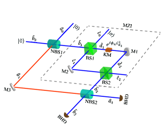
Figure 1: In the dashed box, a standard MZI is input with a coherent state in one input port and one mode of a two-mode squeezed-vacuum state generated by NBS1 in the other input port and is detected with active correlation readout through NBS2. A Kerr-type medium is embedded into one path of the MZI to use as a phase shifter, and the phase transform is $\hat{U}(\phi)=e^{i\phi_{l}\hat{n}_{d_{1}}+i\phi_{n}\hat{n}_{d_{1}}^{2}}$, where $\phi_{l}$ and $\phi_{n}$ represent the linear and nonlinear phase shift, respectively. $\hat{a}_{i}$, $\hat{b}_{i}$, $\hat{c}_{i}$, and $\hat{d}_{i}$ ($i=0,1,2,3$) denote light beams in the different processes. $\mathrm{M}$, mirrors; $\mathrm{BS}$, linear beam splitters; $\mathrm{NBS}$, nonlinear beam splitters; $\mathrm{BHD}$, balanced homodyne detection.

II Model

As shown in Fig. 1, the MZI is in the dashed box, where one input port is injected with a strong field, and another input port is sent with one mode of a two-mode entanglement state generated by NBS1. A Kerr-type medium is embedded into one path of the MZI to use as a phase shifter and introduce the nonlinear phase shift. One of the output fields of the MZI and the other mode of the two-mode squeezed state are combined to realize active correlation output readout.

The four modes in the scheme are described by the annihilation operators $\hat{a}_{i}$, $\hat{b}_{i}$, $\hat{c}_{i}$, and $\hat{d}_{i}$ ($i=0,1,2,3$). The field $\hat{d}_{1}$ passing through the phase shifter will experience both linear and nonlinear phase shifts. The corresponding phase transformation is written as

$$\hat{U}(\phi_{l},\phi_{n})=\exp(i\phi_{l}\hat{n}_{d_{1}}+i\phi_{n}\hat{n}_{d_{1}}^{2}),$$ (1)

where $\phi_{l}$ and $\phi_{n}$ represent the linear and nonlinear phase shift, respectively. $\hat{n}_{d_{1}}$ denotes the photon number operator.

In the Heisenberg picture, after the phase shift the field $\hat{d}_{1}$ is transformed as

$$\hat{d}_{2}=\exp[i\phi_{l}+i\phi_{n}(2\hat{n}_{d_{1}}+1)]\hat{d}_{1},$$ (2)

The two-port input-output relation of the MZI is given by

$$\hat{b}_{2}=\mathcal{M}_{1}\hat{b}_{1}+\mathcal{M}_{0}\hat{c}_{0},\text{ }\hat{c}_{2}=\mathcal{M}_{2}\hat{c}_{0}+\mathcal{M}_{0}\hat{b}_{1},$$ (3)

where

$$\mathcal{M}_{0}=\sqrt{TR}[e^{i\phi_{l}+i\phi_{n}(2\hat{n}_{d_{1}}+1)}-1],\mathcal{M}_{1}=R$$

$$+Te^{i\phi_{l}+i\phi_{n}(2\hat{n}_{d_{1}}+1)},\mathcal{M}_{2}=Re^{i\phi_{l}+i\phi_{n}(2\hat{n}_{d_{1}}+1)}+T.$$ (4)

$R$ and $T$ are the reflectivity and transmissivity of the two BSs, respectively.

Considering one mode of a two-mode entangled state input to the MZI, the scheme is transformed into a three-port input-output interferometer and their relation is described by

$$\hat{a}_{3} =\hat{a}_{0}\mathcal{A}+\hat{b}_{0}^{\dagger}\mathcal{B}+\hat{c}_{0}^{\dagger}\mathcal{C},\text{ }\hat{b}_{3}=\mathcal{D}\hat{a}_{0}^{\dagger}+\mathcal{E}\hat{b}_{0}+\mathcal{F}\hat{c}_{0},$$ (5)

$$\hat{c}_{2} =\mathcal{M}_{2}\hat{c}_{0}+\mathcal{H}\hat{b}_{0}+\mathcal{I}\hat{a}_{0}^{\dagger},$$ (6)

where

$$\mathcal{A} =G_{2}G_{1}+g_{2}g_{1}e^{i\left(\theta_{2}-\theta_{1}\right)}\mathcal{M}_{1}^{\ast},\text{ }\mathcal{B}=G_{2}g_{1}e^{i\theta_{1}}$$

$$+G_{1}g_{2}e^{i\theta_{2}}\mathcal{M}_{1}^{\ast},\text{ }\mathcal{C}=g_{2}e^{i\theta_{2}}\mathcal{M}_{0}^{\ast},\mathcal{H=}G_{1}\mathcal{M}_{0},$$

$$\text{ }\mathcal{D} =G_{1}g_{2}e^{i\theta_{2}}+G_{2}g_{1}e^{i\theta_{1}}\mathcal{M}_{1},\text{ }\mathcal{E}=g_{2}g_{1}e^{i\left(\theta_{2}-\theta_{1}\right)}$$

$$+G_{2}G_{1}\mathcal{M}_{1},\text{ }\mathcal{F}=G_{2}\mathcal{M}_{0},\text{ }\mathcal{I=}g_{1}e^{i\theta_{1}}\mathcal{M}_{0}.$$ (7)

Here, $G_{1}$ and $G_{2}$ are the gain factors of NBS$1$ and NBS$2$, respectively, for wave splitting and recombination with $G_{i}^{2}-g_{i}^{2}=1$ ($i=1,2$). $\theta_{1}$ and $\theta_{2}$ describe the phase shift of the NBS for wave splitting and recombination, respectively.

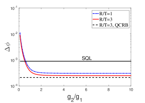
Figure 2: (Color online) The phase sensitivity as a function of $g_{2}/g_{1}$ with different $R/T$ where $|\alpha|=10$ and $g_{1}=2$.

III Estimation of nonlinear phase shift

The Kerr effect in media is usually interpreted as modulation of the refractive index due to the application of a strong drive field. For many materials, the refractive index in the presence of a drive field can be described by Boyd

$$n=n_{0}+n_{2}\langle\hat{I}\rangle,$$ (8)

where $n_{0}$ is the refractive index, $n_{2}$ is a nonlinear coefficient which is proportional to the third-order susceptibility $\chi^{(3)}$ and can be written as $n_{2}=3\chi^{(3)}/4n_{0}^{2}\epsilon_{0}c$, and $\langle\hat{I}\rangle$ is the intensity of the drive field. In our model, the expression of nonlinear phase shift is $\phi_{n}=3\chi^{(3)}\langle\hat{I}_{d_{1}}\rangle k_{d1}L/4n_{0}^{2}\epsilon_{0}c$ with $L$ Kerr media width.

Here, we mainly study the nonlinear phase shift $\phi_{n}$ caused by nonlinear susceptibility $\chi^{(3)}$ changes, since the linear phase shift $\phi_{l}$ is constant. The conceptual understanding of nonlinear optics is often based on the use of the nonlinear susceptibility $\chi^{(3)}$ Boyd14 . Our scheme can give the magnitude of nonlinear susceptibility through the measurement of nonlinear phase shift. The accuracy of nonlinear susceptibility $\chi^{(3)}$ of the Kerr medium is given by phase sensitivity $\Delta\phi_{n}$ measurement, that is

$$\Delta\chi^{(3)}=\frac{4n_{0}^{2}\epsilon_{0}c}{3\langle\hat{I}_{d_{1}}\rangle k_{d1}L}\Delta\phi_{n}.$$ (9)

High sensitivity phase measurement will result in high-precision nonlinear susceptibility measurement. Next, we give the sensitivity of the nonlinear phase shift.

III.1 Homodyne detection

Here, we consider the homodyne detection as our measuring method. The phase sensitivity is described by the relation

$$\Delta^{2}\phi=\frac{\langle\Delta^{2}\hat{O}\rangle}{\left|\partial\langle\hat{O}\rangle/\partial\phi\right|^{2}},$$ (10)

where $\langle\Delta^{2}\hat{O}\rangle$ is the fluctuation of the observable $\hat{O}$, and $\partial\langle\hat{O}\rangle/\partial\phi$ is the slope with respect to the corresponding phase shift. The detected variable can be phase quadrature or the photon number. In our scheme, the observable is phase quadrature $\hat{Y}_{a_{3}}=-i(\hat{a}_{3}-\hat{a}_{3}^{\dagger})$. For convenience, the following $\phi$ all represent nonlinear phase shifts, and we omit the subscript $n$.

The slope of the quadrature $\hat{Y}$ is given by

$$|\partial\langle\hat{Y}_{a_{3}}\rangle/\partial\phi| =|\langle g_{2}[\hat{a}_{0}g_{1}Te^{i(\theta_{2}-\theta_{1}-\phi(2\hat{n}_{d_{1}}+1))}+(\hat{b}_{0}^{\dagger}G_{1}T$$

$$+\hat{c}_{0}^{\dagger}\sqrt{TR})e^{i(\theta_{2}-\phi(2\hat{n}_{d_{1}}+1))}](2\hat{n}_{d_{1}}+1)$$

$$+\text{H.c.}\rangle|.$$ (11)

For convenience, we analyze the phase sensitivity at $\phi=0$. When the two input ports of the SU(1,1) interferometer have no injection, i.e., $\hat{a}_{0}$ and $\hat{b}_{0}$ are in vacuum states, and the pump light is in a coherent state $\left|\alpha\right\rangle$ with $\alpha=|\alpha|e^{i\theta_{\alpha}}$ where $\alpha$ is a complex number and $\theta_{\alpha}$ is the initial phase, then the slope of the quadrature $\hat{Y}$ is reduced to

$$|\partial\langle\hat{Y}_{a_{3}}\rangle/\partial\phi| =2g_{2}\sqrt{TR}N_{\alpha}^{1/2}\left(1+2RN_{\alpha}+4Tg_{1}^{2}\right)$$

$$\times|\cos(\theta_{2}-\theta_{\alpha})|,$$ (12)

where $N_{\alpha}=|\alpha|^{2}$. The increase in the slope of the output signal is due to the amplification of the second nonlinear process and the increase in phase-sensitive photons due to the strong pumping field when $|\cos(\theta_{2}-\theta_{\alpha})|=1$. The corresponding fluctuation is given by

$$\langle\Delta^{2}\hat{Y}_{a_{3}}\rangle =G_{2}^{2}G_{1}^{2}+g_{1}^{2}g_{2}^{2}+G_{2}^{2}g_{1}^{2}+G_{1}^{2}g_{2}^{2}$$

$$+4G_{2}G_{1}g_{1}g_{2}\cos(\theta_{2}-\theta_{1}).$$ (13)

From Eq. (12) and Eq. (13), $R$ and $T$ are only related to the slope and are independent of noise. The optimal $R/T$ is given by

$$\frac{R}{T} =1/(2N_{\alpha}+1)[3N_{\alpha}-6g_{1}^{2}$$

$$+\sqrt{9N_{\alpha}^{2}-28N_{\alpha}g_{1}^{2}+2N_{\alpha}+36g_{1}^{4}+4g_{1}^{2}+1}],$$ (14)

which is independent of $g_{2}$. When the intensity of the input coherent state is strong enough, we obtain the optimal

$$\left(\frac{R}{T}\right)_{optimal}\approx 3,$$ (15)

which is because the nonlinear term $4R\sqrt{TR}N_{\alpha}^{3/2}$ in Eq. (12) dominates in phase sensitivity. Different forms of nonlinear phase shifts produce different $R/T$ optimal ratios. If the nonlinear phase shift is not considered, Eq. (12) can be rewritten as $|\partial\langle\hat{Y}_{a_{3}}\rangle/\partial\phi|=2g_{2}\sqrt{TR}N_{\alpha}^{1/2}|\cos(\theta_{2}-\theta_{\alpha})|$. Under this condition, the optimum value of $R/T$ is $1$, which is the commonly used ratio in the MZI for linear phase-shift estimation.

Our scheme can also be thought of as inserting an MZI into one of the arms of the SU(1,1) interferometer. To illustrate the quantum correlation enhancement effects, we first consider a balanced case $G_{1}=G_{2}$, $\theta_{\alpha}=0$, $\theta_{1}=0$ and $\theta_{2}=\pi$. The phase sensitivity of our scheme is

$$\Delta\phi_{\text{balance}}=\frac{1}{g\left(\mathcal{T}_{Lin}+\mathcal{T}_{Nonlin}+\mathcal{T}_{Nonlin\&Corr}\right)},$$ (16)

where $\mathcal{T}_{Lin}=2\sqrt{TR}N_{\alpha}^{1/2}$, $\mathcal{T}_{Nonlin}=4R\sqrt{TR}N_{\alpha}^{3/2}$, and $\mathcal{T}_{Nonlin\&Corr}=4T\sqrt{TR}N_{\alpha}^{1/2}N_{g}$. $N_{g}=2g^{2}$ is the spontaneous photon number emitted from the NBS, which is related to parametric strength. Additionally, the second NBS further enhances the phase sensitivity by introducing an overall prefactor $g$ to the slope.

If we only consider the MZI in the dashed box, Eq. (16) is simplified to $\Delta\phi_{\text{MZI}}=1/(\mathcal{T}_{Lin}+\mathcal{T}_{Nonlin})$. Furthermore, when the nonlinear phase shift is replaced by the linear phase shift, $\Delta\phi_{\text{MZI}}$ is reduced to $1/\mathcal{T}_{Lin}$. Compared to the usual MZI of linear phase shift, $\mathcal{T}_{Nonlin\&Corre}$ results from the combined action of nonlinear phase shift and quantum correlation created by the first NBS.

Next, we compare the optimal phase sensitivity of our scheme with the SQL. The number of phase-sensing photons of the scheme is

$$N_{ps}=N_{g1}+N_{\alpha},$$ (17)

where $N_{g1}=2g_{1}^{2}$. For a conventional SU(1,1) interferometer with vacuum state input, $N_{ps}$ is $N_{g1}$. The MZI can tolerate a large number of photons $N_{\alpha}$, and the output light does not affect the quantum correlation when the small phase shift around $\phi=0$ is considered. Therefore, the intrinsic problem of a small number of phase-sensing photons is solved. The SQL for the nonlinear phase shift is $1/N_{ps}^{3/2}$ N2 . The phase sensitivity as a function of $g_{2}/g_{1}$ is shown in Fig. 2 at $\phi=0$. When $g_{1}$ and $N_{\alpha}$ are given, the value of $g_{2}/g_{1}$ is $2$ or greater, and the phase sensitivity reaches a stable optimal value. The phase sensitivity obtained by the homodyne detection can beat the SQL.

III.2 Quantum Cramér-Rao bound

The quantum Fisher information (QFI) is the intrinsic information in the quantum state and is not related to the actual measurement procedure. The QFI is at least as great as the classic Fisher information for the optimal observable, which gives an upper limit to the precision of quantum parameter estimation. The QCRB according to the QFI is given by

$$\Delta\phi_{\mathcal{F}}=\frac{1}{\sqrt{m\mathcal{F}}},$$ (18)

where $m$ is the number of independent repeats of the experiment.

The QFI $\mathcal{F}$ is defined as $\mathcal{F}=\mathrm{Tr}[\rho(\phi)L_{\phi}^{2}]$ Braunstein94 ; Braunstein96 , where the Hermitian operator $L_{\phi}$, called the symmetric logarithmic derivative, is defined as the solution of the equation $\partial_{\phi}\rho(\phi)=[\rho(\phi)L_{\phi}+L_{\phi}\rho(\phi)]/2$. In terms of the complete basis $\{|k\rangle\}$ such that $\rho(\phi)=\sum_{k}p_{k}|k\rangle\langle k|$ with $p_{k}\geq 0$ and $\sum_{k}p_{k}=1$, the QFI can be written as $\mathcal{F}=\sum_{k,k^{\prime}}\frac{2}{p_{k}+p_{k^{\prime}}}\left|\langle k|\partial_{\phi}\rho(\phi)|k^{\prime}\rangle\right|^{2}$ Braunstein94 ; Braunstein96 ; Toth . Under the lossless condition, for a pure state, the QFI is reduced to $\mathcal{F}=4(\langle\Psi_{\phi}^{\prime}|\Psi_{\phi}^{\prime}\rangle-|\langle\Psi_{\phi}^{\prime}|\Psi_{\phi}\rangle|^{2})$, where the state after the phase shift is represented as $|\Psi_{\phi}\rangle$ and $|\Psi_{\phi}^{\prime}\rangle=\partial|\Psi_{\phi}\rangle/\partial\phi$.

Under the condition of $g_{1}=g$ and $\ \theta_{1}=0$, and considering the nonlinear phase shift $\hat{d}_{2}=e^{i\phi(2\hat{n}_{d_{1}}+1)}\hat{d}_{1}$, compared to the linear phase shift, the QFI $\mathcal{F}$ is given by

$$\mathcal{F}=4\left[\left\langle\hat{n}_{d_{1}}^{4}\right\rangle-\left\langle\hat{n}_{d_{1}}^{2}\right\rangle^{2}\right]=N_{\alpha}^{3}s_{1}+N_{\alpha}^{2}s_{2}+N_{\alpha}s_{3}+s_{4},$$ (19)

where

$$s_{1} =16R^{4}+16R^{3}T(N_{g}+1),s_{2}=24R^{4}+R^{3}T(88N_{g}$$

$$+48)+R^{2}T^{2}(52N_{g}^{2}+88N_{g}+24),$$

$$s_{3} =4R^{4}+R^{3}T(52N_{g}+12)+R^{2}T^{2}(96N_{g}^{2}+104N_{g}$$

$$+12)+RT^{3}(40N_{g}^{3}+96N_{g}^{2}+52N_{g}+4),$$

$$s_{4} =T^{4}(5N_{g}^{4}+16N_{g}^{3}+13N_{g}^{2}+2N_{g})+T^{3}R(16N_{g}^{3}$$

$$+26N_{g}^{2}+6N_{g})+T^{2}R^{2}(13N_{g}^{2}+6N_{g})+2TR^{3}N_{g}.$$ (20)

If only considering the linear phase shift, the above QFI $\mathcal{F}$ can be reduced to

$$\mathcal{F} =4\left\langle\Delta^{2}\hat{n}_{d_{1}}\right\rangle=N_{\alpha}[4R^{2}+4RT(N_{g}+1)]$$

$$+N_{g}[T^{2}N_{g}+2TR]+2T^{2}N_{g}.$$ (21)

Under the condition of $N_{\alpha}=0$ and $T=R=1/2$, $\mathcal{F}$ is given by $\mathcal{F}=\frac{1}{4}[N_{g}(N_{g}+2)+2N_{g}]$. Compared to the form $N_{g}(N_{g}+2)$ in an SU(1,1) interferometer Li16 , the prefactor $1/4$ results from the introduction of a BS in one arm of the SU(1,1) interferometer, and the extra term $2N_{g}$ is due to the vacuum fluctuation despite $N_{\alpha}=0$.

Next, we compare the QCRB with the SQL, and the phase sensitivity obtained by the homodyne detection. As shown in Fig. 2, the optimal phase sensitivity obtained by homodyne detection can beat the SQL and can approach the QCRB.

IV Losses

In the presence of realistic imperfections, the ultimate precision limit in noisy quantum-enhanced metrology was also studied. In this section, we investigate the effects of losses on phase sensitivities.

IV.1 Internal and external losses of MZI

Losses can be modeled by adding fictitious beam splitters, as shown in Fig. 3. Considering both arms of the MZI have different internal transmission rates $\eta_{c}$ and $\eta_{d}$, and outside transmission rates $\eta_{a}$ and $\eta_{b}$, the mode transforms of the fields are given by

$$\hat{c}_{1}^{\prime} =\sqrt{\eta_{c}}\hat{c}_{1}+\sqrt{1-\eta_{c}}\hat{v}_{c},\text{ }\hat{d}_{2}^{\prime}=\sqrt{\eta_{d}}\hat{d}_{2}+\sqrt{1-\eta_{d}}\hat{v}_{d},$$ (22)

$$\hat{a}_{1}^{\prime} =\sqrt{\eta_{a}}\hat{a}_{1}+\sqrt{1-\eta_{a}}\hat{v}_{a},\text{ }\hat{b}_{2}^{\prime}=\sqrt{\eta_{b}}\hat{b}_{2}+\sqrt{1-\eta_{b}}\hat{v}_{b},$$ (23)

where $\hat{v}_{a}$, $\hat{v}_{b}$, $\hat{v}_{c}$, and $\hat{v}_{d}$ represent the vacuum. Considering the losses, the input-output relation of $\hat{a}_{3}$ is

$$\hat{a}_{3_{l}}=\hat{a}_{0}\mathcal{A}_{l}+\hat{b}_{0}^{\dagger}\mathcal{B}_{l}+\hat{c}_{0}^{\dagger}\mathcal{C}_{l}+\hat{v}_{a}\mathcal{V}_{1}+\hat{v}_{b}^{\dagger}\mathcal{V}_{2}+\hat{v}_{c}^{\dagger}\mathcal{V}_{3}+\hat{v}_{d}^{\dagger}\mathcal{V}_{4},$$ (24)

with

$$\mathcal{A}_{l} =\sqrt{\eta_{a}}G_{2}G_{1}+\sqrt{\eta_{b}}g_{2}g_{1}e^{i\left(\theta_{2}-\theta_{1}\right)}(\sqrt{\eta_{d}}Te^{-i\phi(2\hat{n}_{d_{1}}+1)}$$

$$+\sqrt{\eta_{c}}R),$$

$$\mathcal{B}_{l} =\sqrt{\eta_{a}}G_{2}g_{1}e^{i\theta_{1}}+\sqrt{\eta_{b}}G_{1}g_{2}e^{i\theta_{2}}(\sqrt{\eta_{d}}Te^{-i\phi(2\hat{n}_{d_{1}}+1)}$$

$$+\sqrt{\eta_{c}}R),$$

$$\mathcal{C}_{l} =\sqrt{\eta_{b}}g_{2}e^{i\theta_{2}}\sqrt{TR}(\sqrt{\eta_{d}}e^{-i\phi(2\hat{n}_{d_{1}}+1)}-\sqrt{\eta_{c}}),$$

$$\mathcal{V}_{1} =G_{2}\sqrt{1-\eta_{a}},\text{ }\mathcal{V}_{2}=g_{2}e^{i\theta_{2}}\sqrt{1-\eta_{b}},$$

$$\mathcal{V}_{3} =-g_{2}e^{i\theta_{2}}\sqrt{R}\sqrt{\eta_{b}(1-\eta_{c})},\text{ }$$

$$\mathcal{V}_{4} =g_{2}e^{i\theta_{2}}\sqrt{T}\sqrt{\eta_{b}(1-\eta_{d})},$$ (25)

where subscript $l$ indicates the loss. Similar to the lossless case, we analyze the phase sensitivity at $\phi=0$. At this phase point, the slope is

$$|\partial\langle\hat{Y}_{a_{3_{l}}}\rangle/\partial\phi| =2g_{2}\sqrt{\eta_{b}\eta_{d}TR}N_{\alpha}^{1/2}$$

$$\times\left(1+2RN_{\alpha}+2TN_{g}\right)|\cos(\theta_{2}-\theta_{\alpha})|,$$ (26)

and the fluctuation of the quadrature $\hat{Y}_{a_{3_{l}}}$ is

$$\langle\Delta^{2}\hat{Y}_{a_{3_{l}}}\rangle =\eta_{a}G_{2}^{2}G_{1}^{2}+\eta_{b}g_{2}^{2}g_{1}^{2}\left(\sqrt{\eta_{d}}T+\sqrt{\eta_{c}}R\right)^{2}$$

$$+\eta_{a}G_{2}^{2}g_{1}^{2}+\eta_{b}g_{2}^{2}G_{1}^{2}\left(\sqrt{\eta_{d}}T+\sqrt{\eta_{c}}R\right)^{2}$$

$$+\eta_{b}g_{2}^{2}TR\left(\sqrt{\eta_{d}}-\sqrt{\eta_{c}}\right)^{2}$$

$$+\left[\left(1-\eta_{a}\right)G_{2}^{2}\right]+\left[\left(1-\eta_{b}\right)g_{2}^{2}\right]$$

$$+\left[\eta_{b}\left(1-\eta_{c}\right)g_{2}^{2}R\right]+\left[\eta_{b}\left(1-\eta_{d}\right)g_{2}^{2}T\right]$$

$$+4\sqrt{\eta_{a}\eta_{b}}G_{2}G_{1}g_{1}g_{2}\left(\sqrt{\eta_{d}}T+\sqrt{\eta_{c}}R\right)\cos(\theta_{2}-\theta_{1}).$$ (27)

From the above two equations, the condition for obtaining the optimal phase sensitivity is $\theta_{\alpha}=0$, $\theta_{1}=0$, and $\theta_{2}=\pi$. We can study the effects of internal losses by setting $\eta_{a}=\eta_{b}=1$, or study the effects of the external losses by setting $\eta_{c}=\eta_{d}=1$.

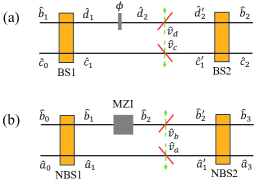
Figure 3: A lossy interferometer model, the losses in the interferometer are modeled by adding fictitious beam splitters. (a) Internal losses. (b) External losses.

For convenience, we first consider $g_{2}=2g_{1}$. The phase sensitivity as a function of photon losses in both arms $\eta_{c}$ and $\eta_{d}$ when $\eta_{a}=\eta_{b}=1$ is shown in Fig. 4(a), where the dashed line denotes $1/N_{ps}^{3/2}$. The phase sensitivities in the upper right corner and within the dashed line area can overcome $1/N_{ps}^{3/2}$. Since the strong pump field injection and the unbalanced BS make the intensity of the upper arm of the MZI larger than that of the lower arm, it is more tolerant with loss of light field $\eta_{d}$. It is shown that the interferometer can tolerate approximately $70\%$ of the photon losses when $\eta_{c}=1$. Similarly, considering external photon losses, the phase sensitivity as a function of photon losses in both arms $\eta_{a}$ and $\eta_{b}$ when $\eta_{c}=\eta_{d}=1$ is shown in Fig. 4(b). It is demonstrated that the phase sensitivity can still overcome $1/N_{ps}^{3/2}$ with $40\%$ of the photon losses. Large photon loss affects quantum correlation, which reduces the sensitivity of measurement.

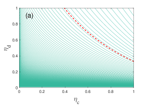
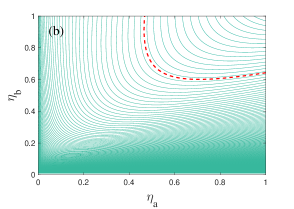
Figure 4: Phase sensitivity vs photon loss coefficient $\eta$, where $|\alpha|=10$, $g_{1}=2$, and $R/T=3$. (a) Internal losses. (b) External losses. The dashed lines denote $1/N_{ps}^{3/2}$. The phase sensitivities in the upper right corner and within the dashed line area can overcome $1/N_{ps}^{3/2}$.

IV.2 Detection losses

Finally, we study the detection loss, and the field undergoing the detection losses is $\hat{a}_{3}^{{}^{\prime}}=\sqrt{\eta}\hat{a}_{3}+\sqrt{1-\eta}\hat{v}$, where $\hat{v}$ is the vacuum. The corresponding slope and variance are

$$|\partial\langle\hat{Y}^{{}^{\prime}}\rangle/\partial\phi_{n}|=2g_{2}\sqrt{TR\eta}N_{\alpha}^{1/2}\left(1+2RN_{\alpha}+4Tg_{1}^{2}\right),$$ (28)

and

$$\langle\Delta^{2}\hat{Y}^{{}^{\prime}}\rangle=\eta[(G_{2}G_{1}-g_{2}g_{1})^{2}+(G_{2}g_{1}-G_{1}g_{2})^{2}]+1-\eta,$$ (29)

respectively. For a balanced configuration ($G_{1}=G_{2}$, $\theta_{\alpha}=0$, $\theta_{1}=0$, and $\theta_{2}=\pi$), this type of loss only introduces a prefactor $1/\sqrt{\eta}$ to the sensitivity, i.e., $\Delta\phi^{\prime}=(\Delta\phi)_{\text{balance}}/\sqrt{\eta}$, which is the same as the result by intensity detection Marino12 .

V Conclusion

In conclusion, we have proposed a scheme to enhance the nonlinear phase estimation of an MZI with a coherent state in one input port and one mode of a two-mode squeezed-vacuum state in the other input port and with active correlation readout. The phase sensitivity is improved compared to the traditional MZI for the same input phase sensing field because of active correlation output readout. Due to introduction of nonlinear phase estimation, the optimal $R/T$ ratio is about $3$ instead of $1$ usually used under the condition of strong coherent-state input. The phase sensitivity can beat the SQL and approach the QCRB using the method of homodyne detection under the condition of the optimal $R/T$ ratio. The internal and external losses of the optical field degraded the measurement precision, and we have given their critical values where the phase sensitivity is below the SQL in the presence of photon losses. The detection loss only introduces a prefactor $1/\sqrt{\eta}$ to the sensitivity for the balanced configuration. Due to the relation between the nonlinear phase shift and the susceptibility $\chi^{(3)}$ of the Kerr medium, our scheme can also provide the estimation of nonlinear susceptibility $\chi^{(3)}$.

VI ACKNOWLEDGMENTS

This work is supported by National Natural Science Foundation of China Grants No. 11974111, No. 11874152, No. 91536114, No. 11574086, NO. 11974116, No. 11654005, and No. 11474095; Development Program of China Grant No. 2016YFA0302001; Natural Science Foundation of Shanghai Grant No. 17ZR1442800; Shanghai Rising-Star Program Grant No. 16QA1401600; and the Fundamental Research Funds for the Central Universities.

References

- (1) J. B. Fixler, G. T. Foster, J. M. McGuirk, and M. A. Kasevich, Atom Interferometer Measurement of the Newtonian Constant of Gravity, Science 315, 74 (2007).
- (2) A. Peters, K. Y. Chung, and S. Chu, High-precision gravity measurements using atom interferometry, Metrologia 38, 25 (2001).
- (3) B. P. Abbott et al. (LIGO Scientific Collaboration and Virgo Collaboration), Observation of Gravitational Waves from a Binary Black Hole Merger, Phys. Rev. Lett. 116, 061102 (2016).
- (4) B. P. Abbott et al. (LIGO Scientific Collaboration and Virgo Collaboration), GW170817: Observation of Gravitational Waves from a Binary Neutron Star Inspiral, Phys. Rev. Lett. 119, 161101 (2017).
- (5) The LIGO Scientific Collaboration, A gravitational wave observatory operating beyond the quantum shot-noise limit, Nat. Phys. 7, 962 (2011).
- (6) C. M. Caves, Quantum-mechanical noise in an interferometer, Phys. Rev. D 23, 1693 (1981).
- (7) M. Xiao, L.-A. Wu, and H. J. Kimble, Precision measurement beyond the shot-noise limit, Phys. Rev. Lett. 59, 278 (1987).
- (8) A. N. Boto, P. Kok, D. S. Abrams, S. L. Braunstein, C. P. Williams, and J. P. Dowling, Quantum Interferometric Optical Lithography: Exploiting Entanglement to Beat the Diffraction Limit, Phys. Rev. Lett. 85, 2733 (2000).
- (9) S. Steinlechner, J. Bauchrowitz, M. Meinders, H. Müller-Ebhardt, K. Danzmann, and R. Schnabel, Quantum-dense metrology, Nat. Photon. 7, 626 (2013).
- (10) B. Yurke, S. L. McCall, and J. R. Klauder, SU(2) and SU(1, 1) interferometers, Phys. Rev. A 33, 4033 (1986).
- (11) J. Jing, C. Liu, Z. Zhou, Z. Y. Ou, and W. Zhang, Realization of a nonlinear interferometer with parametric amplifiers, Appl. Phys. Lett. 99, 011110 (2011).
- (12) F. Hudelist, J. Kong, C. Liu, J. Jing, Z. Y. Ou, and W. Zhang, Quantum metrology with parametric amplifier-based photon correlation interferometers, Nat. Commun. 5, 3049 (2014).
- (13) B. Chen, C. Qiu, S. Chen, J. Guo, L. Q. Chen, Z. Y. Ou, and W. Zhang, Atom-Light Hybrid Interferometer, Phys. Rev. Lett. 115, 043602 (2015).
- (14) C. Qiu, S. Chen, L. Q. Chen, B. Chen, J. Guo, Z. Y. Ou, and W. Zhang, Atom–light superposition oscillation and Ramsey-like atom–light interferometer, Optica 3, 775 (2016).
- (15) D. Linnemann, H. Strobel, W. Muessel, J. Schulz, R. J. Lewis-Swan, K. V. Kheruntsyan, and M. K. Oberthaler, Quantum-Enhanced Sensing Based on Time Reversal of Nonlinear Dynamics, Phys. Rev. Lett. 117, 013001 (2016).
- (16) S. Lemieux, M. Manceau, P. R. Sharapova, O. V. Tikhonova, R. W. Boyd, G. Leuchs, and M. V. Chekhova, Engineering the Frequency Spectrum of Bright Squeezed Vacuum via Group Velocity Dispersion in an SU(1,1) Interferometer, Phys. Rev. Lett. 117, 183601 (2016).
- (17) M. Manceau, G. Leuchs, F. Khalili, and M. Chekhova, Detection Loss Tolerant Supersensitive Phase Measurement with an SU(1,1) Interferometer, Phys. Rev. Lett. 119, 223604 (2017).
- (18) B. E. Anderson, P. Gupta, B. L. Schmittberger, T. Horrom, C. Hermann-Avigliano, K. M. Jones, and P. D. Lett, Phase sensing beyond the standard quantum limit with a variation on the SU(1,1) interferometer, Optica 4, 752 (2017).
- (19) P. Gupta, B. L. Schmittberger, B. E. Anderson, K. M. Jones, and P. D. Lett, Optimized phase sensing in a truncated SU(1,1) interferometer, Opt. Express 26, 000391 (2017).
- (20) W. Du, J. Jia, J. F. Chen, Z. Y. Ou, and W. Zhang, Absolute sensitivity of phase measurement in an SU(1,1) type interferometer, Opt. Lett. 43, 1051 (2018).
- (21) W. N. Plick, J. P. Dowling, and G. S. Agarwal, Coherent-light-boosted, sub-shot noise, quantum interferometry, New J. Phys. 12, 083014 (2010).
- (22) Z. Y. Ou, Enhancement of the phase-measurement sensitivity beyond the standard quantum limit by a nonlinear interferometer, Phys. Rev. A 85, 023815 (2012).
- (23) A. M. Marino, N. V. Corzo Trejo, and P. D. Lett, Effect of losses on the performance of an SU(1,1) interferometer, Phys. Rev. A 86, 023844 (2012).
- (24) D. Li, C.-H. Yuan, Z. Y. Ou, and W. Zhang, The phase sensitivity of an SU (1,1) interferometer with coherent and squeezed-vacuum light, New J. Phys. 16, 073020 (2014).
- (25) M. Gabbrielli, L. Pezzè, and A. Smerzi, Spin-Mixing Interferometry with Bose-Einstein Condensates, Phys. Rev. Lett. 115, 163002 (2015).
- (26) Z.-D. Chen, C.-H. Yuan, H.-M. Ma, D. Li, L. Q. Chen, Z. Y. Ou, and W. Zhang, Effects of losses in the atom-light hybrid SU(1,1) interferometer, Opt. Express 24, 17766 (2016).
- (27) C. Sparaciari, S. Olivares, and M. G. A. Paris, Gaussian-state interferometry with passive and active elements, Phys. Rev. A 93, 023810 (2016).
- (28) D. Li, B. T. Gard, Y. Gao, C.-H. Yuan, W. Zhang, H. Lee, and J. P. Dowling, Phase sensitivity at the Heisenberg limit in an SU(1,1) interferometer via parity detection, Phys. Rev. A 94, 063840 (2016).
- (29) Q.-K. Gong, X.-L. Hu, D. Li, C.-H. Yuan, Z. Y. Ou, and W. Zhang, Intramode correlations enhanced phase sensitivities in an SU(1,1) interferometer, Physical Review A 96, 033809 (2017).
- (30) E. Giese, S. Lemieux, M. Manceau, R. Fickler, and R.W. Boyd, Phase sensitivity of gain-unbalanced nonlinear interferometers, Phys. Rev. A 96, 053863 (2017).
- (31) X.-L. Hu, D. Li, L. Q. Chen, K. Zhang, W. Zhang, and C.-H. Yuan, Phase estimation for an SU(1,1) interferometer in the presence of phase diffusion and photon losses, Phys. Rev. A 98, 023803 (2018).
- (32) S. S. Szigeti, R. J. Lewis-Swan, and S. A. Haine, Pumped-Up SU(1,1) Interferometry, Phys. Rev. Lett. 118, 150401 (2017).
- (33) S. Liu, Y. Lou, J. Xin, and J. Jing, Quantum Enhancement of Phase Sensitivity for the Bright-Seeded SU(1,1) Interferometer with Direct Intensity Detection, Phys. Rev. Applied 10, 064046 (2018).
- (34) R. W. Boyd, G. S. Agarwal, W. V. Davis, A. L. Gaeta, E. M. Nagasako, and M. Kauranen, Quantum noise characteristics of nonlinear optical amplifiers, Acta Physica Polonica A 86, 117(1994).
- (35) M. Kauranen, A. L. Gaeta, and R. W. Boyd, Amplification of vacuum fluctuations by two-beam coupling in atomic vapors, Phys. Rev. A 50, 929(R) (1994).
- (36) W. V. Davis, M. Kauranen, E. M. Nagasako, R. J. Gehr, A. L. Gaeta, and R. W. Boyd, Excess noise acquired by a laser beam after propagating through an atomic-potassium vapor, Phys. Rev. A 51, 4152 (1995).
- (37) C. M. Caves, Reframing SU(1,1) interferometry, Adv. Quantum Technol 123, 1900138 (2020).
- (38) J. Beltrán and A. Luis, Breaking the Heisenberg limit with inefficient detectors, Phys. Rev. A 72, 045801 (2005).
- (39) S. Boixo, A. Datta, M. J. Davis, S. T. Flammia, A. Shaji, and C. M. Caves, Quantum Metrology: Dynamics versus Entanglement, Phys. Rev. Lett. 101, 040403 (2008).
- (40) M. Napolitano, M. Koschorreck, B. Dubost, N. Behbood, R. J. Sewell and M. W. Mitchell, Interaction-based quantum metrology showing scaling beyond the Heisenberg limit, Nature 471, 486 (2011).
- (41) J. Joo, K. Park, H. Jeong, W. J. Munro, K. Nemoto, and T. P. Spiller, Quantum metrology for nonlinear phase shifts with entangled coherent states, Phys. Rev. A 86, 043828 (2012).
- (42) K. Berrada, Quantum metrology with SU(1,1) coherent states in the presence of nonlinear phase shifts, Phys. Rev. A 88, 013817 (2013).
- (43) J. Cheng, Quantum metrology for simultaneously estimating the linear and nonlinear phase shifts, Phys. Rev. A 90, 063838 (2014).
- (44) J.-D. Zhang, Z.-J. Zhang, L.-Z. Cen, J.-Y. Hu, and Y. Zhao, Nonlinear phase estimation: Parity measurement approaches the quantum Cramér-Rao bound for coherent states, Phys. Rev. A 99, 022106 (2019).
- (45) W. Du, J. Kong, J. Jia, S. Ming, C. H. Yuan, J. F. Chen, Z. Y. Ou, M. W. Mitchell, and W. Zhang, SU(2)-in-SU(1,1) nested interferometer, arXiv:2004.14266
- (46) R. W. Boyd, Nonlinear Optics, 3rd ed. (Academic Press, New York, 2008).
- (47) R. W. Boyd, Z. Shi, and I. De Leon, The third-order nonlinear optical susceptibility of gold, Opt. Commun. 326, 74 (2014).
- (48) S. L. Braunstein and C. M. Caves, Statistical distance and the geometry of quantum states, Phys. Rev. Lett. 72, 3439 (1994).
- (49) S. L. Braunstein, C. M. Caves, and G. J. Milburn, Generalized uncertainty relations: Theory, examples, and Lorentz invariance, Ann. Phys. 247, 135 (1996).
- (50) G. Tóth and I. Apellaniz, Quantum metrology from a quantum information science perspective, J. Phys. A 47, 424006 (2014).