Efficient Transformer-based Large Scale Language Representations using Hardware-friendly Block Structured Pruning

Abstract

Pre-trained large-scale language models have increasingly demonstrated high accuracy on many natural language processing (NLP) tasks. However, the limited weight storage and computational speed on hardware platforms have impeded the popularity of pre-trained models, especially in the era of edge computing. In this work, we propose an efficient transformer-based large-scale language representation using hardware-friendly block structure pruning. We incorporate the reweighted group Lasso into block-structured pruning for optimization. Besides the significantly reduced weight storage and computation, the proposed approach achieves high compression rates. Experimental results on different models (BERT, RoBERTa, and DistilBERT) on the General Language Understanding Evaluation (GLUE) benchmark tasks show that we achieve up to 5.0$\times$ with zero or minor accuracy degradation on certain task(s). Our proposed method is also orthogonal to existing compact pre-trained language models such as DistilBERT using knowledge distillation, since a further 1.79$\times$ average compression rate can be achieved on top of DistilBERT with zero or minor accuracy degradation. It is suitable to deploy the final compressed model on resource-constrained edge devices.

1 Introduction

Transformer-based language model pre-training has proven to be highly effective in learning universal language representations from large-scale unlabeled data and being fine-tuned to adapt to downstream tasks Peters et al. (2018); Sun et al. (2019). Representative works such as BERT Devlin et al. (2018), XLNet Yang et al. (2019), RoBERTa Liu et al. (2019b), MT-DNN Liu et al. (2019a), ALBERT Lan et al. (2019), GPT-2 Radford et al. , and UniLMv2 Bao et al. (2020) have substantially advanced the state-of-the-art across a variety of downstream tasks, such as text classification, natural language inference, and question answering.

Despite its success in performance improvement in natural language understanding and generation, the computational cost and data storage of Transformer-based pre-trained language model are two widely recognized concerns due to Transformer’s deep architecture and rich parameters. These models typically contain several hundred million parameters. The recent released research models even reach multi-billion parameters, such as MegatronLM (8.3 billion parameters) Shoeybi et al. (2019), Turing-NLG (17 billion parameters) Microsoft (2020) and GPT-3 (175 billion parameters) Brown et al. (2020), which require more advanced computing facility. Hence, it is imperative to reduce the computational cost and model storage of pre-trained Transformer-based language models in order to popularize their applications in computer systems, especially in edge devices with limited resources.

Several works have been developed in the context of model compression, such as knowledge distillation Hinton et al. (2015); Sanh et al. (2019); Jiao et al. (2019); Sun et al. (2019), weight pruning Han et al. (2015), parameter sharing Lan et al. (2019) and weight quantization Polino et al. (2018). For computer vision, the information compressed/reduced in image features can be partially retrieved from neighboring pixels since they share similar and uniform characteristics spatially. However, for NLP, the syntax and semantics information of Transformer in language/text domain are more sensitive than that of computer vision. A high compression rate for large-scale language models is difficult to achieve on downstream NLP tasks. As a result, there are few works in exploring and optimizing hardware-friendly model compression techniques for state-of-the-art Transformer-based pre-trained language models, to reduce the weight storage and computation on computer system while maintaining prediction accuracy.

In this work, we propose an efficient Transformer-based large-scale language representations using block structured pruning. The contributions of this work are as follows.

• To the best of our knowledge, we are the first to investigate hardware-friendly weight pruning on pre-trained large-scale language models. Besides the significantly reduced weight storage and computation, the adopted block structure pruning has high flexibility in achieving a high compression rate. The two advantages are critical for efficient Transformer in NLP since the non-uniformed syntax and semantics information in language/text domain makes weight pruning more difficult than computer vision.

• We incorporate the reweighted group Lasso for optimization into block structured pruning-based on pre-trained large-scale language models including BERT, RoBERTa, and DistilBERT. We relax the hard constraints in weight pruning by adding regularization terms in the objective function and use reweighted penalty parameters for different blocks. The dynamical regularization technique achieves higher compression rate with zero or minor accuracy degradation.

• Our proposed method is orthogonal to existing compact pre-trained language models such as DistilBERT using knowledge distillation. We can further reduce the model size using our method with zero or minor accuracy.

We evaluate the proposed approach on several GLUE benchmark tasks Wang et al. (2018). Experimental results show that we achieve high compression rates with zero or minor accuracy degradation. With significant gain in weight storage reduction (up to 5$\times$) and computation efficiency, our approach can maintain comparable accuracy score to original large models including DistilBERT. The hardware-friendly transformer-based acceleration method is suitable to be deployed on resource-constrained edge devices.

2 Related Work

To address the memory limitation and high computational requirement of commonly seen deep learning platforms such as graphics processing unit (GPU), tensor processing unit (TPU) and field-programmable gate array (FPGA) on large-scale pre-trained language models, various of compact NLP models or model compression techniques have been investigated. ALBERT Lan et al. (2019) utilizes parameter sharing technique across encoders to reduce weight parameters and uses the same layer structures as BERT. It achieves comparable results on different benchmarks to BERT. Despite the weight storage reduction, the computational overhead remains unchanged since ALBERT and BERT have the same network structure.

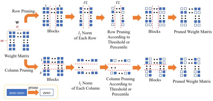
Figure 1: Block structured pruning for weight matrix.

Knowledge distillation is another type of model compression technique, which distills the knowledge from a large teacher model or an ensemble of models to a light-weighted student model Hinton et al. (2015). The student model is trained to intimate the class probabilities produced by the large teacher model. For instance, DistilBERT Sanh et al. (2019) applies knowledge distillation to BERT, and achieves 1.67 $\times$ model size reduction and 1.63 $\times$ inference speedup, while retaining 97% accuracy on the dev sets on the GLUE benchmark, compared to BERT. Patient knowledge distillation Sun et al. (2019) is used to learn from multiple intermediate layers of the teacher model for incremental knowledge extraction.

Efficient deep learning methods can reduce the model size and accelerate the computation. It is well known that, in practice, the weight representation in deep learning models is redundant. After removing several redundant weights with appropriate model compression algorithms, the deep learning model can have minor accuracy degradation. Prior work focused on heuristic and iterative non-structured magnitude weight pruning (a.k.a, irregular pruning) Han et al. (2015). It causes overhead in both weight storage and computation in computer systems. On weight storage, it results in irregular, sparse weight matrices (as arbitrary weights can be pruned), and relies on indices to be stored in a compressed format such as Coordinate (COO) format. The introduced indices cause extra memory footprint, i.e., at least one index per non-zero value, further degrading the compression rate. On computation, it is difficult to be accelerated on current GPU architectures as reported in Han et al. (2016); Wen et al. (2016); Yu et al. (2017). On the other hand, structured pruning considers regularity in weight pruning focusing on generating regular but smaller and dense matrix with no index. However, it suffers notable accuracy loss due to the poor solution quality, and therefore not suitable for pruning sensitive syntax and semantics information in Transformer.

3 Block Structured Pruning

3.1 Problem Formulation

We adopt a more fine-grained block structured pruning algorithm, where pruning is executed by excluding entire blocks of weights within weight matrices such as rows or columns, therefore significantly reducing the number of indices when storing on memory. On computation, it is compatible with parallel computing platforms such as GPUs or Field Programmable Gate Arrays (FPGAs) in implementing matrix multiplications. We formulate the weight pruning problem using reweighted group Lasso, to orchestrate the block structured pruning. Thus, the Transformer-based large-scale models can be more efficient on computer systems while satisfying the accuracy requirement. As shown in Figure 1, we divide the weight matrix into small blocks and apply row pruning and column pruning on each block. For each row/column block, we compute the $l_{2}$ norm. We prune the weights within the block according to our pre-set threshold or percentile. The pseudocode is shown in Algorithm 1.

Consider an $N$-layer Transformer, we denote the weights and biases of the $n$-th layer as $\mathbf{W}_{n}$ and $\mathbf{b}_{n}$. The loss function is $f\big{(}\{{\mathbf{W}}_{n}\}_{n=1}^{N},\{{\mathbf{b}}_{n}\}_{n=1}^{N}\big{)}$, which will be minimized during training. For the block structured pruning problem, our target objective is to reduce the number of columns and rows in the blocks of weight matrix while maintaining the prediction accuracy.

minimize $$\quad f\big{(}\{{{\bf W}_{n}}\}_{n=1}^{N},\{{{\bf b}_{n}}\}_{n=1}^{N}\big{)}$$ (1)

subject to    # of non-zero block rows in $${\bf W}_{n} r_{n}$$ is less than

   # of non-zero block columns in $${\bf W}_{n} c_{n}$$ is less than

Algorithm 1 Block structured pruning

  Input: weight matrix $\mathbf{W}$, matrix width $n$, matrix height $m$, row division $k$ (or column division $k^{\prime}$), threshold $t_{b}$

  Output: pruned weight matrix $\mathbf{W}_{p}$

  Set $\mathbf{W}_{p}$ = $\mathbf{W}$

  Divide $\mathbf{W}_{p}$ into $k$ matrices: $\mathbf{W}_{1}$,$\mathbf{W}_{2}$,…,$\mathbf{W}_{k}$

  Set $l_{2}\_norms$ = $zeros(k,m)$

  for $i=1$ to $k$  do

     for $j=1$ to $m$  do

        $l_{2}\_norms(i,j)$ equals the $l_{2}$ norm of the $j$ th row of $\mathbf{W}_{i}$

        if $l_{2}\_norms(i,j)\leq t_{b}$ then

           $\mathbf{W}_{i}$($j$,:) = 0

        end if

     end for

  end for

  $\mathbf{W}_{p}$ = concatenate($\mathbf{W}_{1}$,$\mathbf{W}_{2}$,…,$\mathbf{W}_{k}$)

where $r_{n}$ and $c_{n}$ are the desired non-zero block rows and columns, respectively. Due to regularity in pruning, only the non-zero rows/columns at the block level need to be indexed, as opposed to each non-zero element in irregular pruning. The storage overhead is minor compared to non-structured irregular pruning Han et al. (2016). Because structured pruning is applied independently within each block, the scheme has higher flexibility, thereby higher accuracy, compared to the straightforward application on the whole weight matrix Wen et al. (2016).

3.2 Reweighted Group Lasso Optimization

In problem (1), we use hard constraints to formulate the block row/column pruning problem. However, it is more difficult to satisfy the hard constraints on NLP than on computer vision. There are two reasons: i) Information compressed in image features can be partially retrieved from neighboring pixels since spatially they share similar and uniform characteristics, whereas syntax and semantics information in deep Transformer in language/text domain are not uniformly characterized; ii) Intuitively, the high-level semantic, syntax, and language understanding capability might be broken when we prune zero or near-zero weights in the latent space. Therefore, a high compression rate for large-scale language models is difficult to achieve on downstream NLP tasks.

To address this issue, we relax the hard constraints by adding regularization terms in the objective function. Prior work SSL Wen et al. (2016) uses group Lasso as the relaxation of the hard constraints. Inspired by Candes et al. (2008), we use reweighted penalty parameters for different blocks to achieve a high compression rate under same accuracy requirement than using a fixed penalty parameter to all the blocks in group Lasso method.

When we use group Lasso for block row pruning, the regularization term is

$$\sum_{n=1}^{N}\sum_{i=1}^{p_{n}}\sum_{\alpha=1}^{q_{n}}\sqrt{\sum_{j=(\alpha-1)h_{n}+1}^{\alpha h_{n}}(\mathbf{W}_{n})_{ij}^{2}}$$

where $h_{n}$ is the block row size in the $n$-th layer, $p_{n}$ is the number of rows in $\mathbf{W}_{n}$, $q_{n}$ is the number of blocks in a row of $\mathbf{W}_{n}$. And the block row pruning problem is

$$\underset{\{{{\mathbf{W}}}_{n}\},\{{\mathbf{b}}_{n}\}}{\text{min}}\ \ \ f\big{(}\{{{\mathbf{W}}}_{n}\}_{n=1}^{N},\{{{\mathbf{b}}}_{n}\}_{n=1}^{N}\big{)}$$ (2)

$$+\lambda\sum_{n=1}^{N}\sum_{i=1}^{p_{n}}\sum_{\alpha=1}^{q_{n}}\gamma_{i,\alpha}\sqrt{\sum_{j=(\alpha-1)h_{n}+1}^{\alpha h_{n}}(\mathbf{W}_{n})_{ij}^{2}},$$

where $\lambda$ is the penalty parameter. $\gamma_{i,\alpha}$ is the penalty weight corresponding to the $\alpha$-th block in the $i$-th row, and it is updated by $\gamma_{i,\alpha}={1}/({\sqrt{\sum_{j=(\alpha-1)h_{n}+1}^{\alpha h_{n}}({\bf{\mathbf{W}}}_{n})_{ij}^{2}}+\epsilon})$, where $\epsilon$ is a small value preventing division by zero. Similarly, when we prune columns in a block, the problem becomes

$$\underset{\{{\mathbf{W}}_{n}\},\{{\mathbf{b}}_{n}\}}{\text{min}}\ \ \ f\big{(}\{{\mathbf{W}}_{n}\}_{n=1}^{N},\{{\textbf{{b}}}_{n}\}_{n=1}^{N}\big{)}$$ (3)

$$+\lambda\sum_{n=1}^{N}\sum_{j=1}^{r_{n}}\sum_{\beta=1}^{s_{n}}\gamma_{j,\beta}\sqrt{\sum_{i=(\beta-1)d_{n}+1}^{\beta d_{n}}(\textbf{W}_{n})_{ij}^{2}},$$

where $d_{n}$ is the block column size in the $n$-th layer, $r_{n}$ is the number of columns in $\textbf{W}_{n}$. $s_{n}$ is the number of blocks in a column of $\textbf{W}_{n}$. $\gamma_{j,\beta}$ is the penalty weight corresponding to the $\beta$-th block in the $j$-th column, and it is updated by $\gamma_{j,\beta}={1}/({\sqrt{\sum_{i=(\beta-1)d_{n}+1}^{\beta d_{n}}(\mathbf{W}_{n})_{ij}^{2}}+\epsilon}).$

Algorithm 2 Reweighted group Lasso on Transformer pruning

  Input: pre-trained model, model weight matrix $\mathbf{W}$, matrix width $n$, matrix height $m$

  Set milestones = $m_{1}$, $m_{2}$, …, $m_{s}$

  Set $T_{1}$ as the number of iterations of reweighted training method

  Set $T_{2}$ as the number of iterations of retraining method

  Calculate $\gamma$

  for $s=1$ to $T_{1}$  do

     if $s$ in milestones then

        Update $\gamma$

     end if

     Calculate $l_{1loss}$ and prediction loss $f(\textbf{W},\textbf{b})$

     $mixed_{loss}=l_{1loss}+f(\textbf{W},\textbf{b})$

     Update model weight $\mathbf{W}$ to minimize $mixed_{loss}$ using Adam

  end for

  Prune the weight matrix $\mathbf{W}$ using block structured pruning

  $Mask=zeros(m,n)$

  for $i=1$ to $m$  do

     for $j=1$ to $n$  do

        if $\textbf{W}_{i,j}==0$ then

           Set $Mask_{i,j}$ = 0

        else

           Set $Mask_{i,j}$ = 1

        end if

     end for

  end for

  for $s=1$ to $T_{2}$  do

     Calculate the prediction loss $f(\mathbf{W},\mathbf{b})$

     Update model weight $\mathbf{W}$ to minimize $f(\textbf{W},\textbf{b})$ using Adam

     $\textbf{W}=\textbf{W}*Mask$

  end for

We start with a pre-trained model and initialize the collection of penalty weights ($\gamma_{i,\alpha}$ or $\gamma_{j,\beta}$) using the parameters in the pre-trained model. We remove the rows or blocks in a block if their group $l_{2}$ norm is smaller than a threshold after reweighted training. We refine the Transformer models using the non-zero weights. $\lambda$ is used for adjusting regularization strength. When $\lambda$ is too small, the reweighted training is close to the original training. When $\lambda$ is too large, it gives too much penalty on the weights and accuracy cannot be maintained. Specifically, we start reweighted training with $\lambda=0$ to reproduce the original results and increase $\lambda$ to derive sparsity of the weight matrices. We stop increasing $\lambda$ when the reweighted training accuracy drops slightly and the accuracy will be improved after retraining. Overall, using the same training trails, our method can achieve higher pruning rate than prior works using structured pruning Wen et al. (2016), as shown in Algorithm 2.

4 Evaluation

4.1 Datasets

We conduct experiments on GLUE benchmark Wang et al. (2018), a comprehensive collection of nine natural language understanding tasks covering three NLP task categories with different degrees of difficulty and dataset scales: single-sentence tasks, paraphrase similarity matching tasks, and inference tasks. All datasets are public available. More specifically, for single-sentence task, we consider the Corpus of Linguistic Acceptability (CoLA) Warstadt et al. (2018), which contains 10,657 sentences of English acceptability judgments from books and articles on linguistic theory, and the Stanford Sentiment Treebank (SST-2) Socher et al. (2013), which is comprised of 215,154 phrases in the parse trees of 11,855 sentences from movie reviews with annotated emotions.

For paraphrase similarity matching tasks, we consider the Microsoft Research Paraphrase Corpus (MRPC) Dolan and Brockett (2005), which contains 5,800 sentence-pairs corpora from online news sources and are manually annotated where the sentences in the sentence-pairs are semantically equivalent; the Semantic Textual Similarity Benchmark (STS-B) Cer et al. (2017), a collection of 8,628 sentence pairs extracted from the news title, video title, image title, and natural language inference data; and the Quora Question Pairs (QQP) , a collection of 400,000 lines of potential question duplicate pairs from the Quora website.

For inference tasks, we consider the Multi-Genre Natural Language Inference Corpus (MNLI) Williams et al. (2018), a set of 433k premise hypothesis pairs to predict whether the premise statement contains assumptions for the hypothesis statement; Question-answering NLI (QNLI) Wang et al. (2018), a set of over 100,000+ question-answer pairs from SQuAD Rajpurkar et al. (2016); The Recognizing Textual Entailment datasets (RTE) Wang et al. (2018), which come from the PASCAL recognizing Textual Entailment Challenge; and Winograd NLI (WNLI) Levesque et al. (2012), a reading comprehension task that comes from the Winograd Schema Challenge.

In all GLUE benchmarks, we report the metrics following the conventions in Wang et al. (2018), i.e., accuracy scores are reported for SST-2, QNLI, RTE, and WNLI; Matthews Correlation Coefficient (MCC) is reported for CoLA; F1 scores are reported for QQP and MRPC; Spearman correlations are reported for STS-B.

4.2 Experimental Setup

Baseline Models. Our baseline models are unpruned BERT_BASE Devlin et al. (2018), RoBERTa_BASE Liu et al. (2019b), and DistilBERT Sanh et al. (2019). As shown in Table 1, for each transformer model, we list the reported accuracy/metrics from the original papers in the first row. We report our reproduced results using the same network architectures in the second row.

Table 1: Comparison of test accuracy using different transformer models among the nine GLUE benchmark tasks.

Models	MNLI	QQP	QNLI	SST-2	CoLA	STS-B	MRPC	RTE	WNLI
BERTBASE Devlin et al. (2018)	84.6	91.2	90.5	93.5	52.1	85.8	88.9	66.4	-
BERTBASE (ours)	83.9	91.4	91.1	92.7	53.4	85.8	89.8	66.4	56.3
BERTBASE prune (ours)	82.9	90.7	88.2	89.3	52.6	84.6	88.3	63.9	56.3
Compression rate	1.428$\times$	1.428$\times$	1.428$\times$	1.428$\times$	1.428$\times$	1.428$\times$	1.428$\times$	1.428$\times$	2.0$\times$
RoBERTaBASE Liu et al. (2019b)	87.6	91.9	92.8	94.8	63.6	91.2	90.2	78.7	-
RoBERTaBASE (ours)	87.8	91.6	93.0	94.7	60.1	90.2	91.1	77.3	56.3
RoBERTa prune (ours)	86.3	87.0	90.0	89.2	55.3	88.8	90.2	74.0	56.3
Compression rate	1.428$\times$	1.428$\times$	1.428$\times$	1.428$\times$	1.246$\times$	1.428$\times$	1.428$\times$	1.428$\times$	2.0$\times$
DistilBERT Sanh et al. (2019)	82.2	88.5	89.2	91.3	51.3	86.9	87.5	59.9	56.3
DistilBERT (ours)	81.9	90.2	89.5	90.9	50.7	86.5	89.8	59.2	56.3
DistilBERT prune (ours)	78.5	87.4	85.3	85.3	53.4	83.7	89.1	59.2	56.3
Compression rate	2.0$\times$	1.667$\times$	1.667$\times$	2.0$\times$	1.197$\times$	1.667$\times$	1.207$\times$	2.0$\times$	2.0$\times$

Evaluation Metrics. To evaluate our proposed framework on NLP model compression problems, we apply our method on different transformer-based models including BERT_BASE, RoBERTa_BASE, and DistilBERT. Reweighted $l_{1}$ training is carried out to add $l_{1}$ regularization, block structured pruning to obtain a sparse model, and retraining to improve the final accuracy.

We access the GPU-AI (Bridges GPU Artificial Intelligence) nodes on the Extreme Science and Engineering Discovery Environment (XSEDE) Towns et al. (2014). We use two node types: Volta 16 - nine HPE Apollo 6500 servers, each with 8 NVIDIA Tesla V100 GPUs with 16 GB of GPU memory each, connected by NVLink 2.0; Volta 32 - NVIDIA DGX-2 enterprise research AI system tightly coupling 16 NVIDIA Tesla V100 (Volta) GPUs with 32 GB of GPU memory each, connected by NVLink and NVSwitch. We also use an $8\times$ NVIDIA Quadro RTX 6000 GPU server with 24 GB of GPU memory each for training. We conduct the experiments using HuggingFace Transformer toolkit for the state-of-the-art NLP Wolf et al. (2019) and the DeepLearningExamples repository from NVIDIA  NVIDIA (2020). Our experiments are performed on Python 3.6.10, GCC 7.3.0, PyTorch 1.4.0, and CUDA 10.1.

We show the prediction accuracy with respect to different compression rates and we evaluate our method on the GLUE benchmark Wang et al. (2018) in Table 1. For BERT, we use the official BERT_BASE, uncased model as our pre-trained model. There are 12 layers ($L$ =12; hidden size $H$ = 768; self-attention heads $A$ = 12), with total number of parameters 110 Million. We use the same fine-tuning hyperparameters as the paper Devlin et al. (2018). For RoBERTa Liu et al. (2019b), we use the official RoBERTa_BASE model as our pre-trained model. It has the same structure as the BERT_BASE model, with 12 layers ($L$=12; hidden size $H$= 768; self-attention heads $A$= 12), and a total number of 125 Million parameters. For DistilBERT Sanh et al. (2019), a distilled model from the BERT_BASE, uncased checkpoint, is used as the pre-trained model. The parameters are $L$ = 6; $H$ = 768; $A$ = 12; total parameters = 66 M. The block size used for pruning has different types, e.g., 3$\times$3, 3$\times$12, and 12$\times$3.

4.3 Implementation Details

We first fine-tune the pre-trained models for classification. BERT, RoBERTa, and DistilBERT share the same steps. We add a single linear layer on top of each original model. We train the model for the nine downstream GLUE tasks with their corresponding datasets. As we feed the data, the entire pre-trained model and the additional untrained classification layer is trained on our specific task. The original layers already have great English words representation, and we only need to train the top layer, with a bit of tweaking in the lower levels to accommodate our task.

For fine-tuning, we run 4 epochs with initial learning rate of $2e^{-5}$, batch size of 32 and warm up proportion of 0.1. For block structured pruning, we adjust the reweighted penalty parameter, compression rate and training steps for each task. We use the same parameters as fine-tuning (epochs, learning rate, batch size), then we adjust some parameters for each task, depending on the prediction performance. For BERT_BASE, we set penalty factor $1e^{-3}$ for WNLI and MRPC; penalty factor $1e^{-4}$ for CoLA, QQP, MNLI, SST-2, and RTE; penalty factor $1e^{-5}$ for QNLI. The learning rate is $3e^{-5}$ and batch size is 32 on nine tasks. For RoBERTa_BASE, we set penalty factor $1e^{-3}$ for WNLI; penalty factor $1e^{-4}$ for MRPC, QQP, SST-2, and RTE; penalty factor $1e^{-5}$ for QNLI, CoLA, and MNLI. The learning rate and batch size are the same as BERT_BASE. For DistilBERT model, the hyperparamters for reweighted training and retraining are learning rate = $3e^{-5}$ and batch size = 128 on nine datasets. We adjust other parameters, including penalty factors, number of blocks, and compression ratios to achieve the satisfied performance on each task.

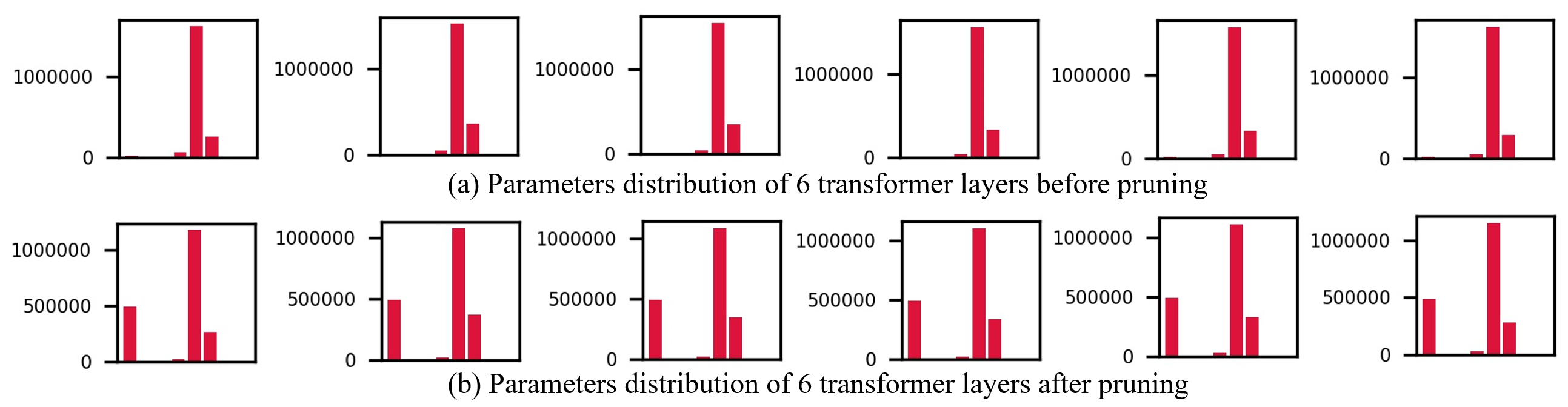
Figure 2: Parameters distribution of DistilBERT model on CoLA dataset: (a) before pruning, (b) after pruning.

We consider three objectives: weight distribution, loss, and accuracy. Weight distribution shows the distribution of weights in each layer after training and retraining. We visualize the weight parameters in Figure 2. With different pruning hyper-parameters including penalty factors, learning rate, block numbers, and compression rate, the weights are distributed differently. We look at two losses: reweighted loss and mixed loss (the object function in Equation (3)). For all our tasks, BERT_BASE, RoBERTa_BASE, and DistilBERT are converged in less than 4 epochs. During training, we evaluate the performance between each given steps.

4.4 Experimental Results

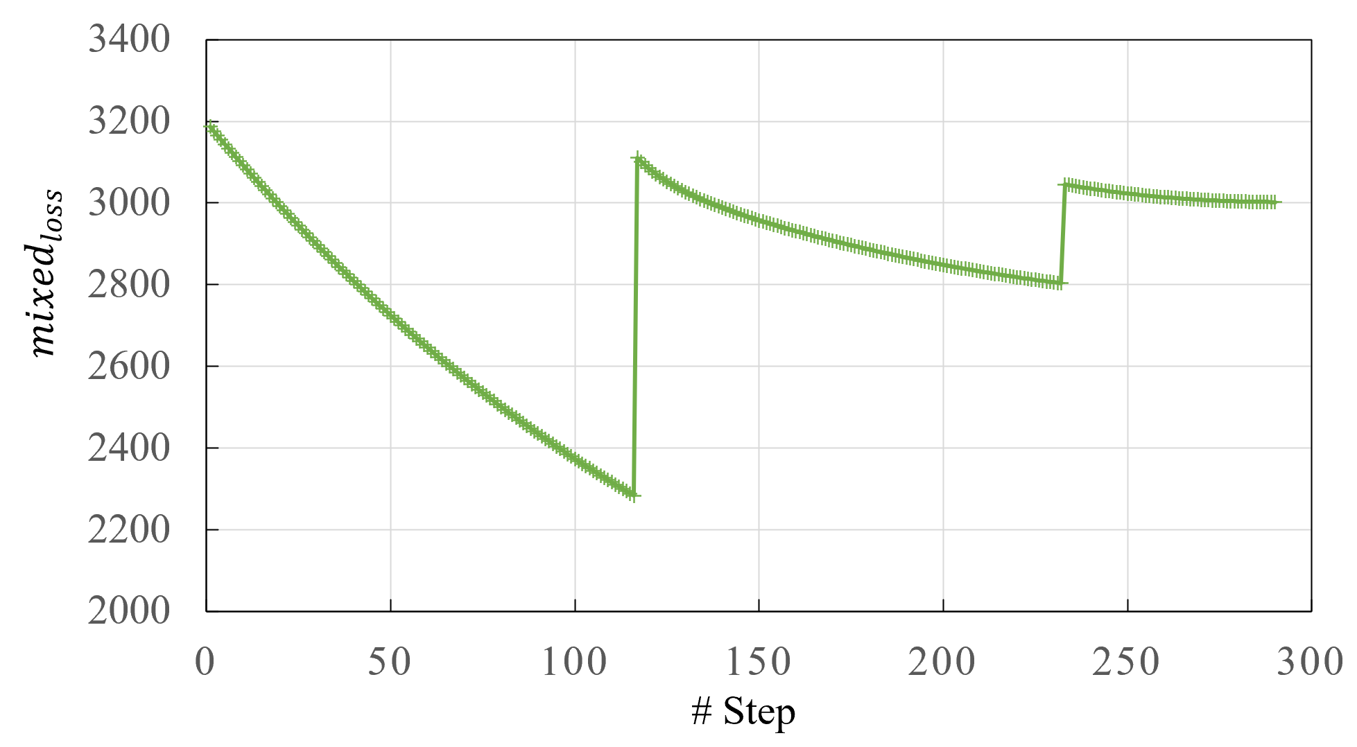
Figure 3: Mixed loss of reweighted training on MRPC dataset with DistilBERT model.

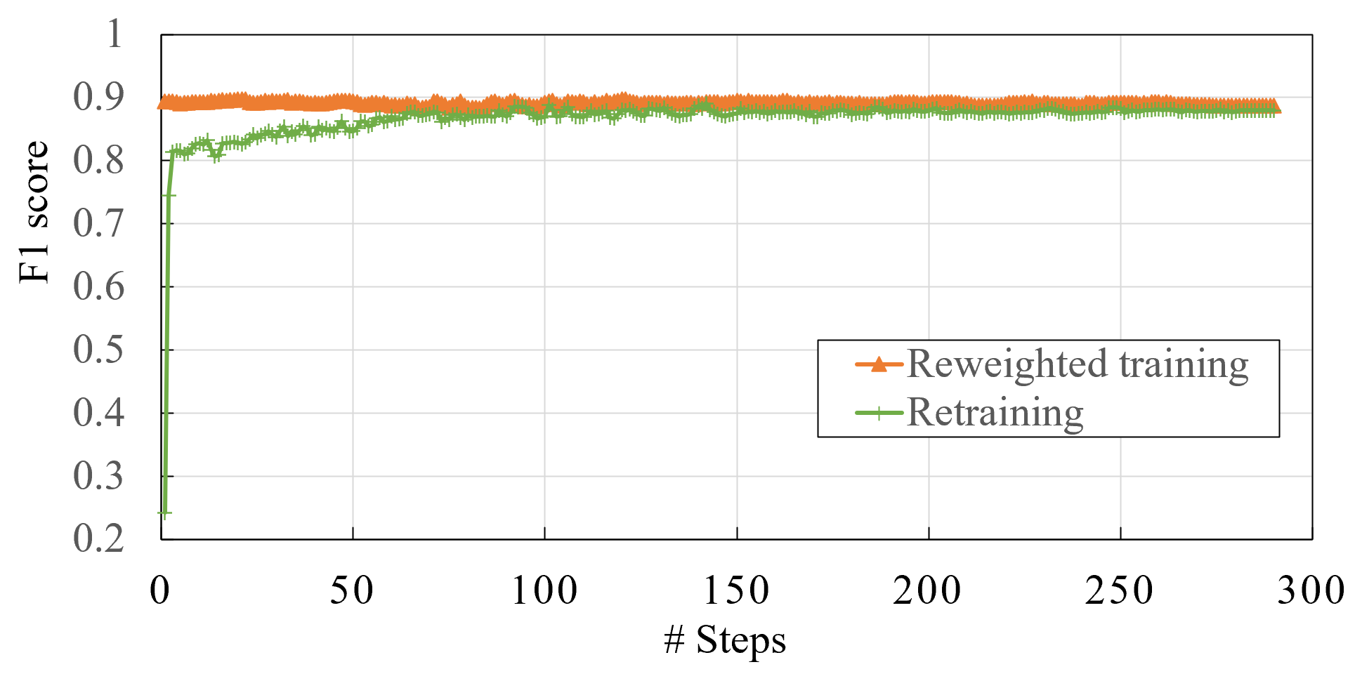
Figure 4: F1 score of reweighted training and retraining with DistilBERT model on MRPC dataset.

We compare the performance (accuracy score) of our pruned models with the baselines. The results are shown in Table 1. For BERT_BASE, we set a compression rate of 1.428$\times$ (i.e., 30% sparsity) or above. The average accuracy degradation is within 2% on all tasks. On WNLI task, there is no accuracy loss. On MNLI, QQP, CoLA, STS-B, and MRPC tasks, the accuracy loss is within 1.5%. On SST-2, QNLI, and RTE tasks, the accuracy loss is also small (within 2.9%), compared to two baseline models. For RoBERTa, the average accuracy degradation is within 3% on all tasks. There is no accuracy loss on WNLI. The accuracy loss is within 1% on MRPC, within 2% on MNLI and STS-B tasks, within 4% on QNLI and RTE tasks, around 5% on QQP, SST-2 and CoLA tasks. For DistilBERT, the average accuracy degradation is within 5% on all tasks. The accuracy losses are within 1% on MRPC task, 3% on MNLI, QQP, QNLI, and STS-B tasks, and 5% on SST-2 task. On CoLA and WNLI datasets, the pruned models perform even better than the unpruned models and increase the final accuracy by 3% (1.197$\times$ compression rate) and 4% (2.0$\times$ compression rate), respectively. Figure 3 and Figure 4 show the reweighted training and retraining results on MRPC dataset, respectively. We choose 256 as the number of blocks. For reweighted training, the mixed loss drops during training within every 116 steps (4 epochs) and increases significantly since we update the penalty matrix $\gamma$. For retraining, the pruned model achieves higher F1 score than the unpruned one.

Table 2: Pruning results of BERT_BASE with different compression rates.

Compression rate	QQP	MNLI	WNLI	QNLI	SST-2
1$\times$	91.4	83.9	56.3	91.1	92.7
1.428$\times$	90.7	82.9	56.3	88.2	89.3
2.0$\times$	90.0	81.2	56.3	85.5	87.0
5.0$\times$	86.9	76.6	56.3	79.5	82.3

We evaluate the accuracy changes when compression rates are different on BERT_BASE and report the accuracy scores for different tasks. Results indicate that the sensitivities of tasks vary significantly under different levels of compression rates. As shown in Table 2, different tasks show different accuracy degradation when using the same compression rate. As we increase the compression rate, the accuracy degradation increased. For specific task (e.g., WNLI), we can achieve up to 5$\times$ compression rate from baseline model with zero accuracy loss. Results on tasks such as WNLI and QQP show minor accuracy degradation while results on SST-2, MNLI, QNLI, show higher accuracy degradation when compression rate is 5.0$\times$. The different accuracy results are related to different dataset sizes, degrees of difficult, and evaluation metrics.

Table 3: Comparison of test accuracy between our BSP method and irregular sparse format on GLUE benchmarks.

Network Model	MNLI	QQP	QNLI	SST2	SSTB	RTE	WNLI
BERTBASE prune	82.9	90.7	88.2	89.3	84.6	63.9	56.3
Prune ratio	1.428$\times$	1.428$\times$	1.428$\times$	1.428$\times$	1.428$\times$	1.428$\times$	2.0$\times$
BERTBASE irregular	83.7	86.5	87.8	90.8	86.7	63.5	56.3
Prune ratio	2.0$\times$	2.0$\times$	1.667$\times$	2.0$\times$	2.5$\times$	2.373$\times$	2.0$\times$
DistilBERT prune	78.5	87.4	85.3	85.3	83.7	59.2	56.3
Prune ratio	2.0$\times$	1.667$\times$	1.667$\times$	2.0$\times$	1.667$\times$	2.0$\times$	2.0$\times$
DistilBERT irregular	80.3	88.7	87.2	86.7	84.7	59.9	56.3
Prune ratio	2.381$\times$	2.174$\times$	2.326$\times$	2.222$\times$	2.222$\times$	2.083$\times$	2.0$\times$

We compare our BSP method with irregular sparse format and the block sparse format Narang et al. (2017); Gray et al. (2017) (pruning all weights on selected blocks). Table 3 shows that under same accuracy, our method achieves a slightly lower pruning ratio compared to irregular sparse format. This is because irregular pruning has a larger flexibility in pruning. However, irregular pruning is less effective when applying to hardware. Irregular sparse format introduces significant memory storage overhead when using Coordinate Format (COO) storage format, therefore is not hardware-friendly. Our method, block structured format (pruning a portion of rows/columns on each block) strikes a better balance between accuracy and memory storage than irregular sparse format or block sparse format Narang et al. (2017); Gray et al. (2017). For irregular sparse format, when storing or transmitting an irregular sparse matrix using the COO format, we store the subsequent nonzeros and related coordinates in memory. Three vectors are needed: row, col, data, where data[i] is value at (row[i], col[i]) position. More specifically, given $50\%$ sparsity for a $8\times 8$ matrix with block size of 4$\times$4, the storage of COO format is $1.5\times 8\times 8=96$; the storage of block structured sparsity (row only) is $8*8\times 0.5+16$ =48. Table 4 lists the accuracy of our method and block sparse format using DistilBERT. Our method achieves $3.04\%$ higher accuracy in average compared with block sparse format.

Table 4: Comparison of test accuracy between our BSP method and block sparse method Narang et al. (2017) on GLUE benchmarks.

Network Model	MNLI	QQP	QNLI	SST2	SSTB	RTE	WNLI
DistilBERT	81.9	90.2	89.5	90.9	86.5	59.2	56.3
DistilBERT-prune	78.5	87.4	85.3	85.3	83.7	59.2	56.3
Block Sparse	78.3	87.2	85.2	83.9	82.2	58.8	49.3
Accuracy Loss	0.2	0.2	0.1	1.4	1.5	0.4	13

As the proposed pruning is hardware-friendly, the pruned weights can be efficiently stored in hardware memory with minor overhead (compared to other pruning methods like irregular pruning). We use a compiler-assisted acceleration framework other than sparse linear algebra libraries, which allows the model to speed up with a sparsity of 30%. We also apply matrix reorder and compact model storage to achieve speed up on edge devices Ma et al. (2020). Hence, it is suitable to deploy the final compressed model on resource-constrained edge devices such as embedded systems and mobile devices.

5 Ablation Studies

In this section, we perform ablation experiments over several parameters when pruning BERT and DistilBERT to better understand their relative importance and the procedure. We change the selection of following parameters: the numbers of blocks for reweighted training and block structured pruning, retraining epochs, and penalty factors. We also evaluate the knowledge distillation friendly.

5.1 Number of Blocks

After selecting penalty factor $3e^{-4}$ and compression rate 2.0$\times$ for each layer (except embedding layers), we choose different numbers of blocks to test. As shown in Table 5, the final accuracy is significantly improved for both BERT_BASE and DitilBERT when we increase the number of blocks. It verifies that with more number of blocks (smaller block size), our weight pruning algorithm has higher flexibility in exploring model sparsity.

Table 5: Number of blocks for reweighted training and retraining on CoLA dataset.

Number of blocks	8	128	256	768
BERTBASE retraining MCC	14.5	48.0	52.6	51.5
DistilBERT retraining MCC	32.2	43.8	47.2	53.4

5.2 Number of Retraining Epochs

By default, all GLUE tests are carried out by running four epochs for pre-training. For reweighted training and retraining, more epochs usually lead to better final accuracy. In this test, we try different reweighted training and retraining epochs. During reweighted training, the mixed loss will drop significantly within every 4 epochs, while the evaluation loss keeps relatively stable. We summarize the results in Table 6. The final accuracy of retraining is improved when we increase the training epochs.

Table 6: Retraining epochs on STS-B dataset.

Number of epochs	4	8	16
BERTBASE retraining Spearman	84.2	84.4	84.6
DistilBERT retraining Spearman	74.6	79.1	80.9

5.3 Penalty Factors

The reweighted training procedure is utilized to penalize the $l_{2}$ norm of the blocks and thus to reduce the magnitude of the weights. Therefore, larger penalty factors help to achieve better retraining accuracy since more smaller weight values of the weight matrices are pruned. However, if the penalty factors are too large, the reweighted training algorithm is not able to compress the model well, which leads to significant accuracy degradation. The results are summarized in Table 7. The retraining accuracy is improved when we increase the penalty factor from $3e^{-5}$ to $1e^{-4}$ and declines from $3e^{-4}$ to $1e^{-3}$.

Table 7: Penalty selections on MNLI dataset.

Penalty factor for each layer	$3e^{-5}$	$1e^{-4}$	$3e^{-4}$	$1e^{-3}$
BERTBASE retraining accuracy	80.7	82.5	82.9	78.9
DistilBERT retraining accuracy	65.8	68.8	73.6	70.0

5.4 Variance of results on multiple runs

During our training, the random seeds are set to 42 as default. We further conduct experiments choosing different seeds and list the results in Table 8. We observe our reported accuracy is aligned with the results with different seeds.

Table 8: Variance of results on multiple runs.

Seed	SST-2	CoLA	STS-B	MRPC
42(default)	85.3	53.4	83.7	89.1
1	83.14	53.75	83.19	89.3
1000	82.8	54.08	83.32	89.3
5000	82.91	54.22	83.03	89.0

5.5 Knowledge Distillation Friendly

To evaluate the effectiveness of our pruning method on distilled models, we focus on the BERT and DistilBERT results in Table 1, where DistilBERT is a highly distilled version of BERT. The average compression rate of BERT and DistilBERT are 1.49$\times$ and 1.79$\times$, respectively. Please note that model size of BERT is 1.67$\times$ of DistilBERT, and therefore is 2.99$\times$ of the final compressed DistilBERT model size. This show that the proposed block structured pruning is orthogonal to knowledge distillation. With this knowledge distillation friendly property, we can first apply the standard knowledge distillation step to reduce the original large model and then apply the proposed pruning method to further reduce the size of the student model.

6 Conclusion

In this work, we propose an hardware-friendly block structured pruning pruning framework for transformer-based large-scale language representation. We incorporate the reweighted group Lasso into for optimization and relax the hard constraints in block structured pruning. We significantly reduce weight storage and computational requirement. Experimental results on different models (BERT, RoBERTa, and DistilBERT) on the GLUE benchmark tasks show that we achieve significant compression rates with zero or minor accuracy degradation on certain benchmarks. Our proposed method is orthogonal to existing compact pre-trained language models such as DistilBERT using knowledge distillation. It is suitable to deploy the final compressed model on resource-constrained edge devices.

7 Appendix

7.1 Single-layer Sensitivity

Before retraining, block structured pruning is carried out for the reweighted trained models by choosing compression ratio for each layer. However, the sensitivity of different layers are different, which may leads to significant accuracy loss if the compression ratios are not proper. To test the sensitivity, we prune 50% of each layer while keeping the other layers unpruned and obtain the final accuracy after retraining. According to tests, embedding layers are sensitive on all datasets except WNLI. On MRPC and RTE datasets, we choose 8 as the number of blocks and $3e^{-4}$ as the penalty factor. In Figure 5, the first two weight matrices are related to embedding layers, while the third to the 38-th weights are related to transformer layers (each transformer layer includes 6 weights). The last two layers is related to classifier layers. The results show that the embedding layers and linear weights in transformer layers are sensitive on CoLA and MRPC datasets. Therefore, we set the compression ratios of corresponding weights zero to ensure the final accuracy.

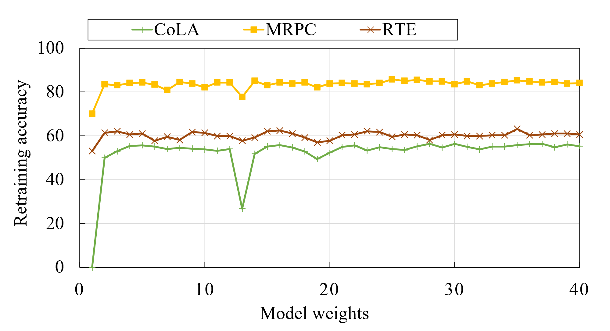
Figure 5: Layer sensitivity with DistilBERT model.

7.2 Number of Blocks

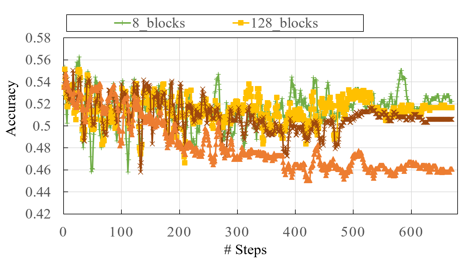
Figure 6: Reweighted training accuracy of different weight matrix block division on CoLA dataset with DistilBERT model.

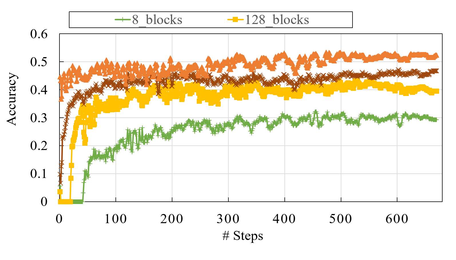
Figure 7: Retraining accuracy of different weight matrix block division on CoLA dataset with DistilBERT model.

Figure 6 and Figure 7 represent reweighted training and retraining accuracy of different block sizes, respectively. During reweighted training, the accuracy decreases when we increase the number of blocks, since the corresponding $l_{1}$ loss increases significantly, which leads to $mixed_{loss}$ to increase as shown in Figure 8. The final accuracy is improved when increasing the number of blocks since the algorithm is capable to operate on smaller units of the weight matrices.

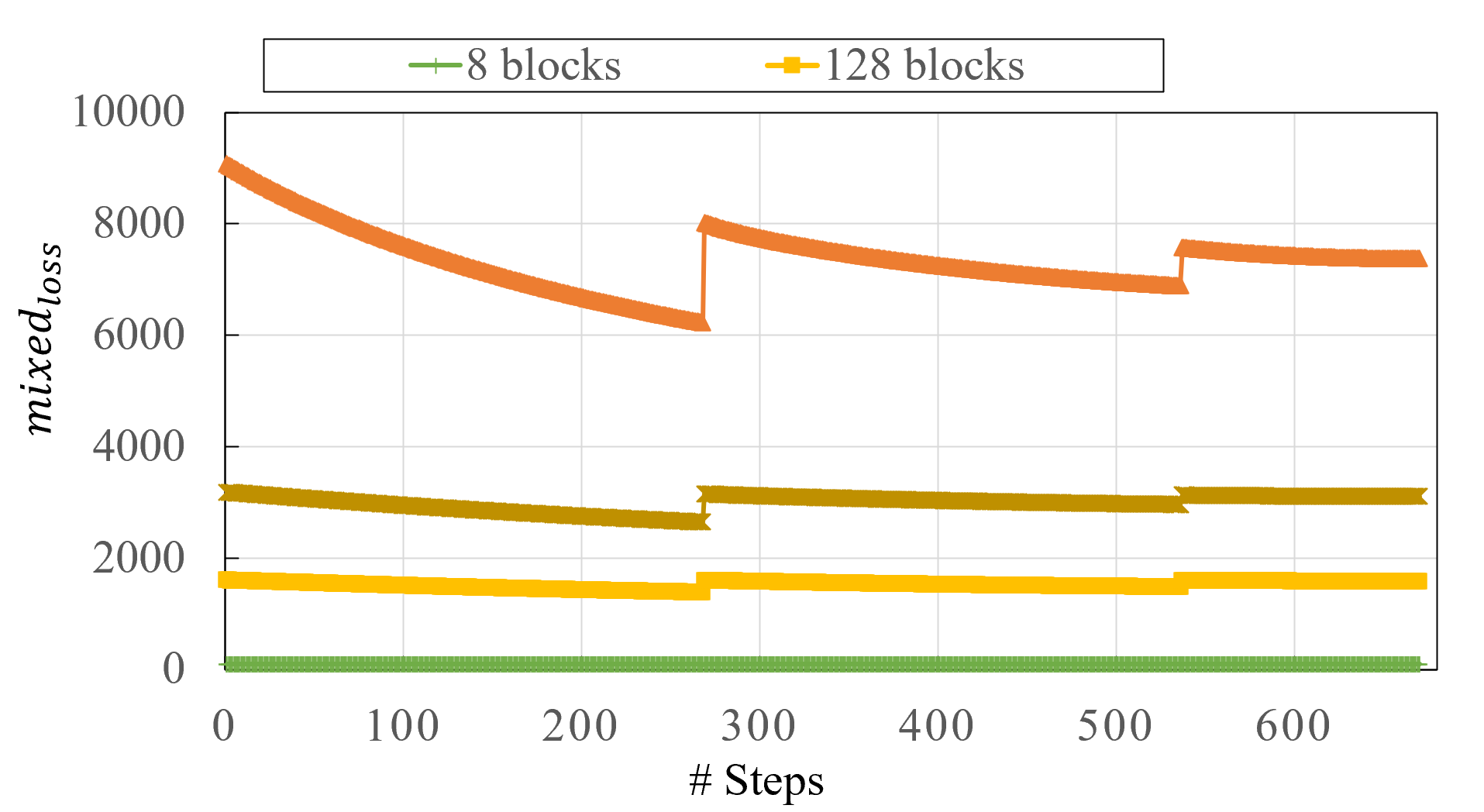
Figure 8: Mixed loss during reweighted training of different weight matrix block divisions on CoLA dataset with DistilBERT model.

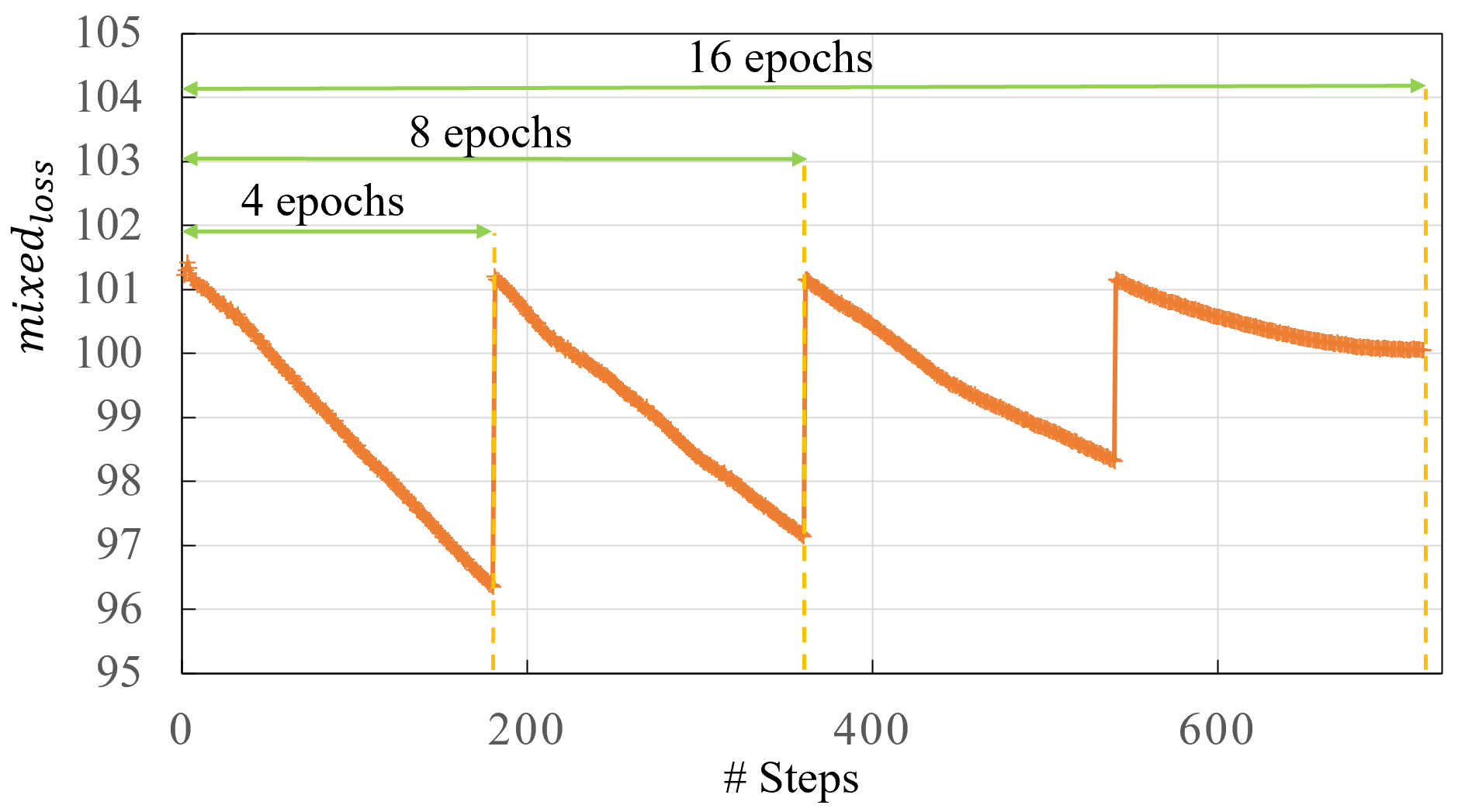
Figure 9: Mixed loss of reweighted training with different epochs on STS-B dataset with DistilBERT model.

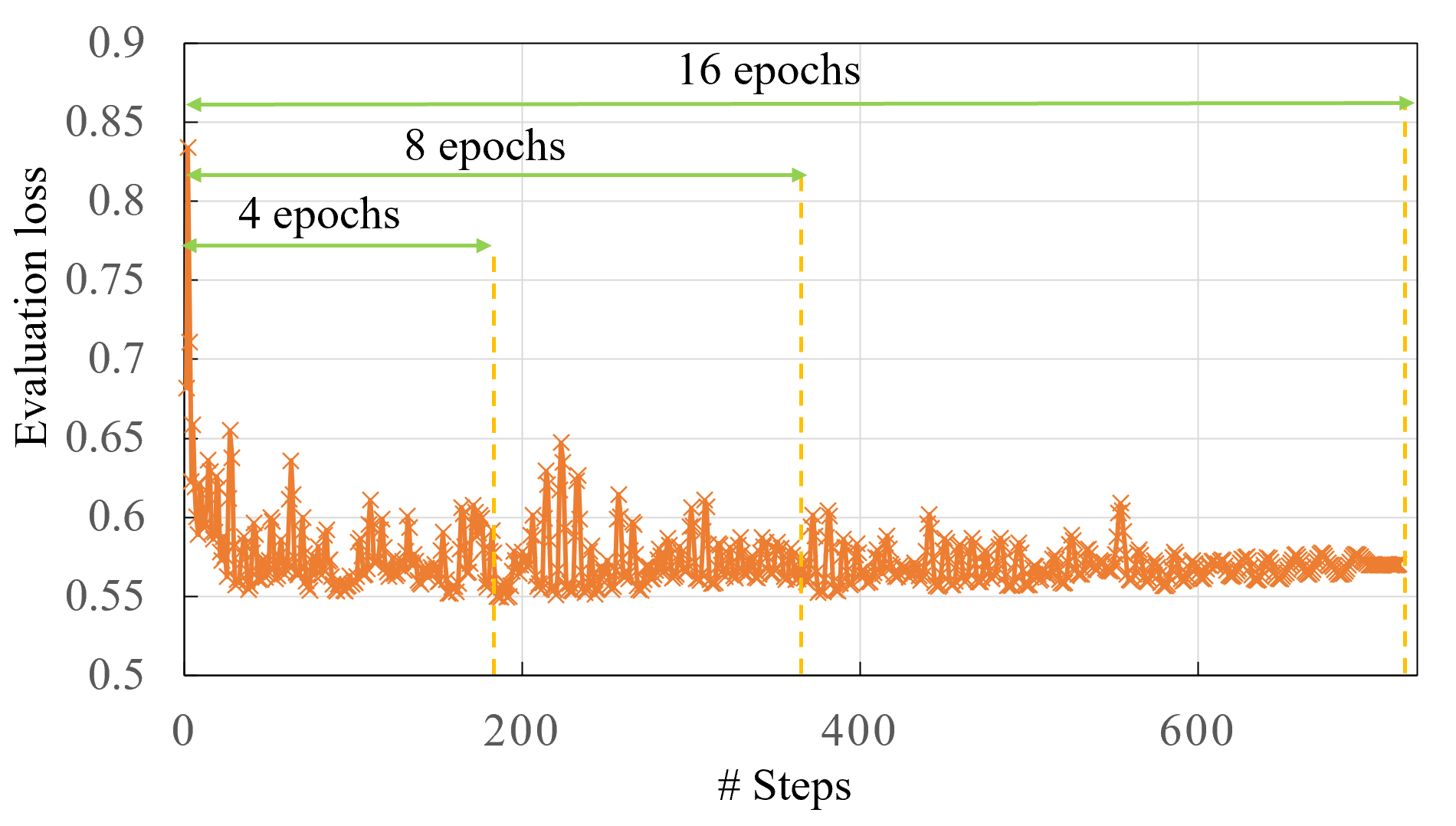
Figure 10: Evaluation loss of reweighted training with different epochs on STS-B dataset with DistilBERT model.

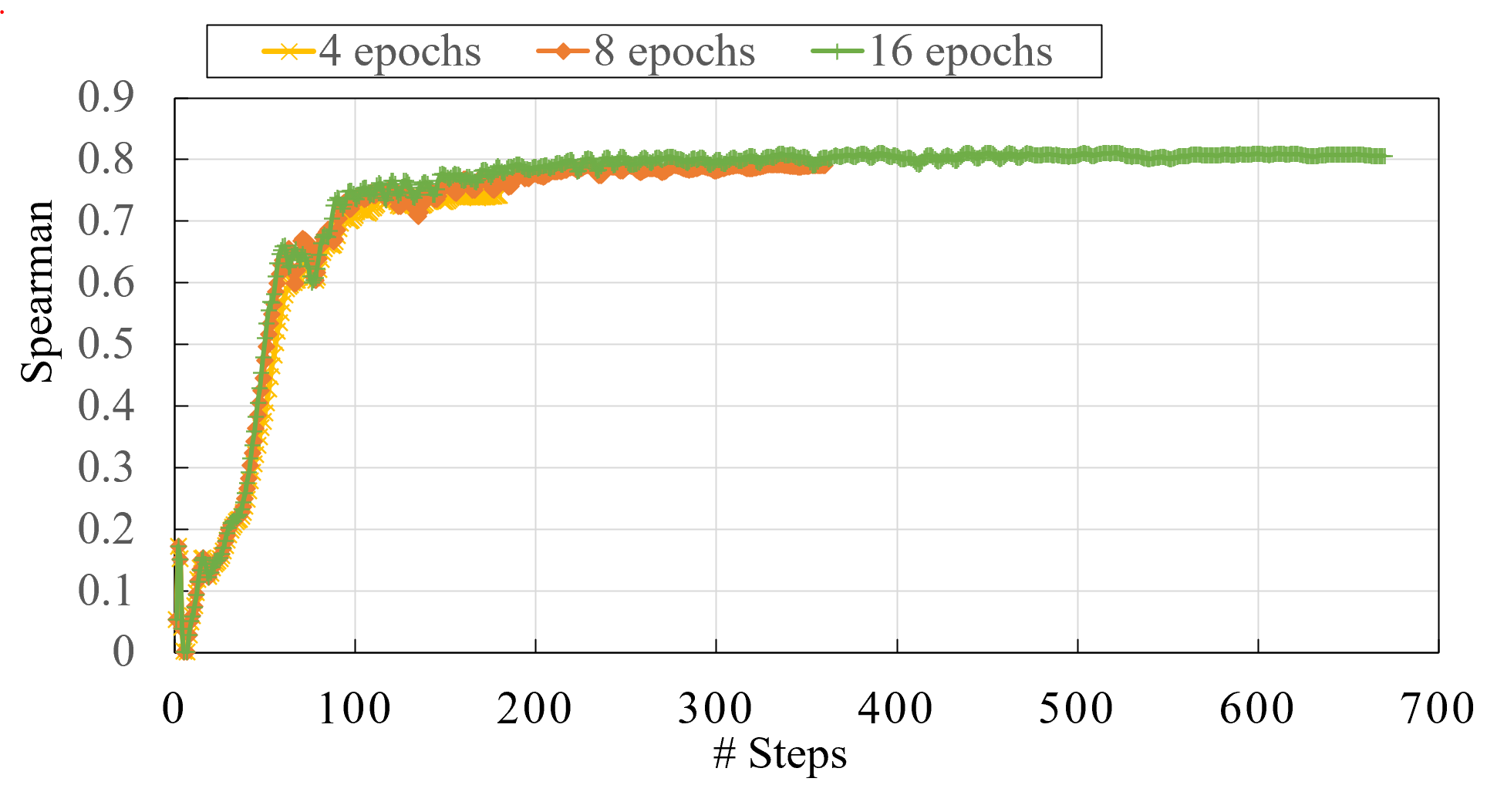
Figure 11: Retraining spearman correlation with different retraining epochs on STS-B dataset with DistilBERT model.

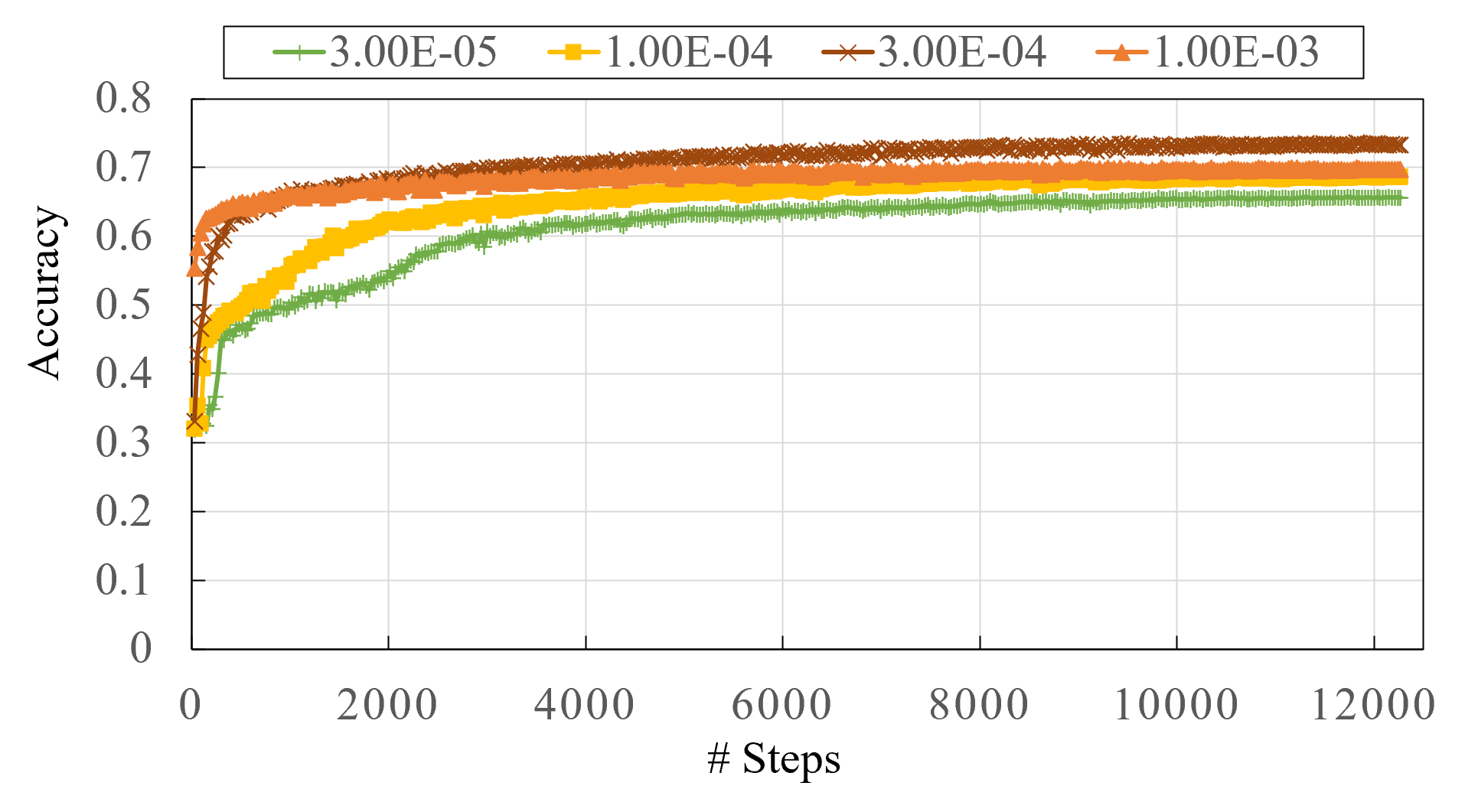
Figure 12: Retraining accuracy using different penalty factors on MNLI dataset with DistilBERT model.

7.3 Number of Retraining Epochs

For reweighted training, Figure 9 and Figure 10 show the results of mixed and evaluation loss, respectively, in which we update the $\gamma$ matrix every four epochs. For each selection of training epochs, we use linear learning rate decay and thus the results do not coincide with each other. The final accuracy of retraining is improved when we increase the training epochs as shown in Figure 11.

7.4 Penalty Factors

In Figure 12, the retraining accuracy is improved when we increase the penalty factor from $3e^{-5}$ to $1e^{-4}$ and declines from $3e^{-4}$ to $1e^{-3}$.

7.5 Retrain Accuracy

Figure 13 $\sim$ Figure 21 show the accuracy with RoBERTa_BASE model on nine GLUE benchmark tasks during retraining steps.

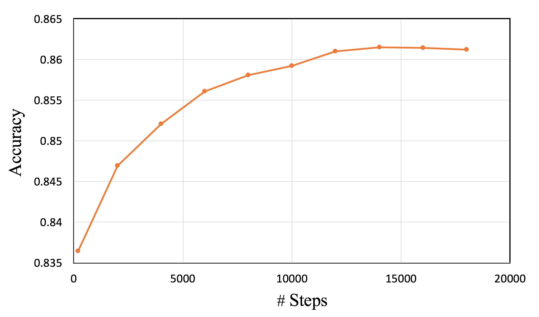
Figure 13: Retraining accuracy on MNLI dataset with RoBERTa model.

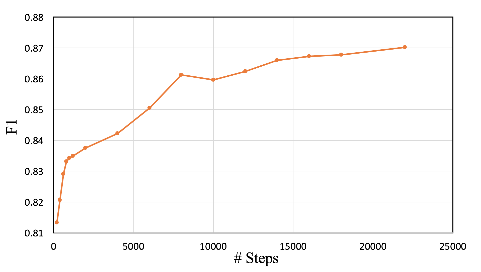
Figure 14: Retraining F1 on QQP dataset with RoBERTa model.

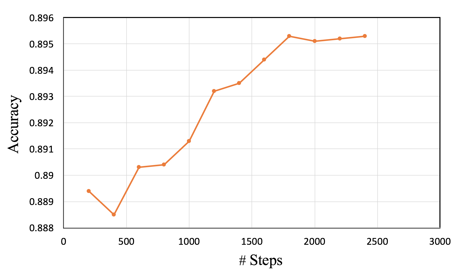
Figure 15: Retraining accuracy on QNLI dataset with RoBERTa model.

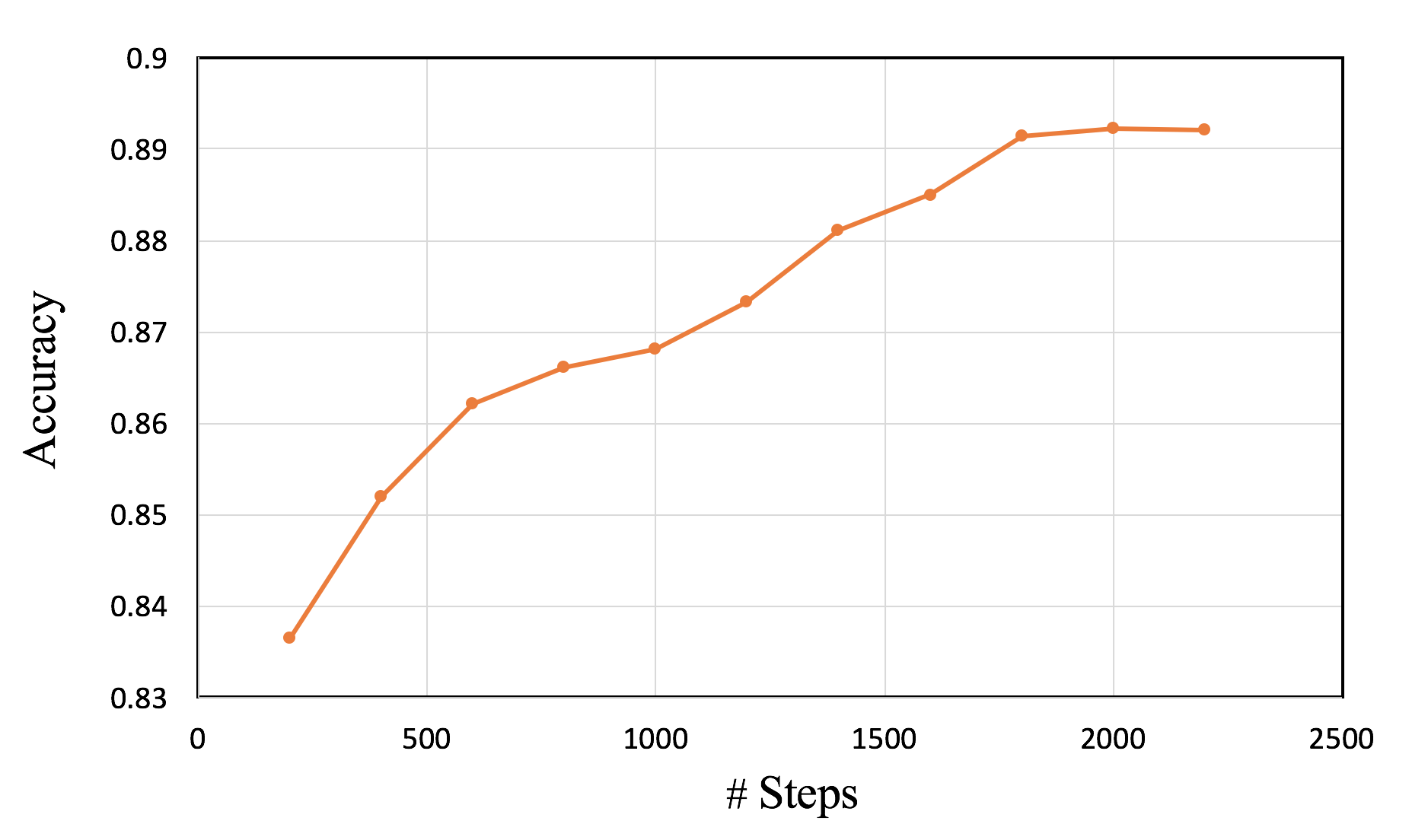
Figure 16: Retraining accuracy on SST-2 dataset with RoBERTa model.

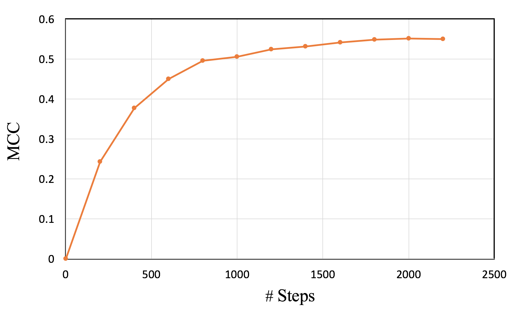
Figure 17: Retraining mcc on CoLA dataset with RoBERTa model.

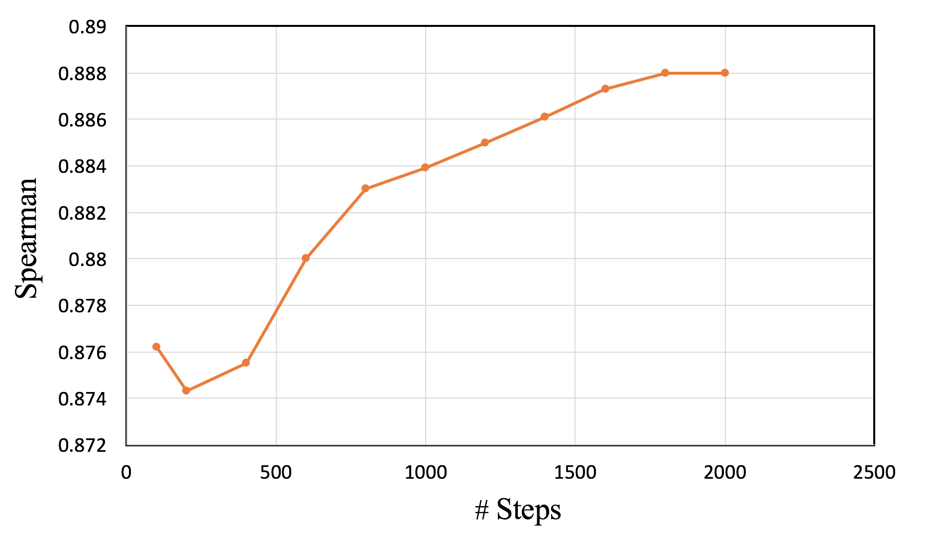
Figure 18: Spearman correlation on STS-B dataset with RoBERTa model.

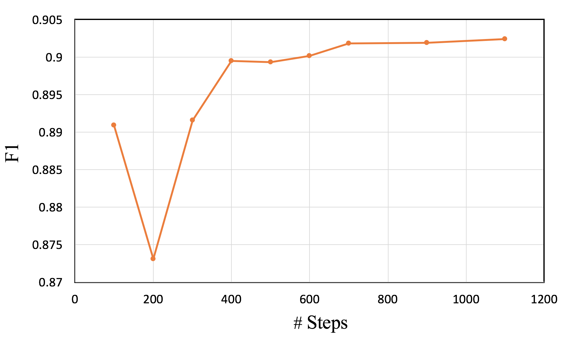
Figure 19: Retraining F1 on MRPC dataset with RoBERTa model.

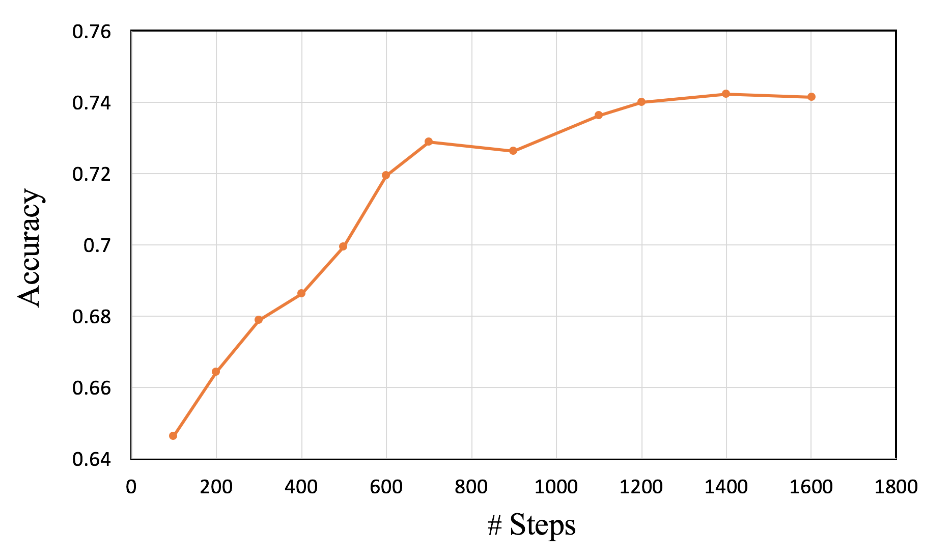
Figure 20: Retraining accuracy on RTE dataset with RoBERTa model.

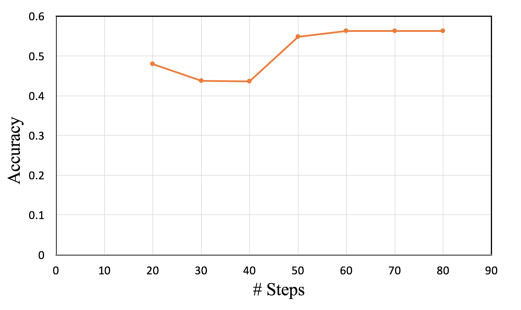
Figure 21: Retraining accuracy on WNLI dataset with RoBERTa model.

References

- Bao et al. (2020) Hangbo Bao, Li Dong, Furu Wei, Wenhui Wang, Nan Yang, Xiaodong Liu, Yu Wang, Songhao Piao, Jianfeng Gao, Ming Zhou, et al. 2020. Unilmv2: Pseudo-masked language models for unified language model pre-training. arXiv preprint arXiv:2002.12804.
- Brown et al. (2020) Tom B. Brown, Benjamin Pickman Mann, Nick Ryder, Melanie Subbiah, Jean Kaplan, Prafulla Dhariwal, Arvind Neelakantan, Pranav Shyam, Girish Sastry, Amanda Askell, Sandhini Agarwal, Ariel Herbert-Voss, G. Krüger, Tom Henighan, Rewon Child, Aditya Ramesh, Daniel M. Ziegler, Jeffrey Wu, Clemens Winter, Christopher Hesse, Mark Chen, Eric J Sigler, Mateusz Litwin, Scott Gray, Benjamin Chess, Jack Clark, Christopher Berner, Sam McCandlish, Alec Radford, Ilya Sutskever, and Dario Amodei. 2020. Language models are few-shot learners.
- Candes et al. (2008) Emmanuel J Candes, Michael B Wakin, and Stephen P Boyd. 2008. Enhancing sparsity by reweighted l1 minimization. Journal of Fourier analysis and applications, 14(5-6):877–905.
- Cer et al. (2017) Daniel Cer, Mona Diab, Eneko Agirre, Iñigo Lopez-Gazpio, and Lucia Specia. 2017. SemEval-2017 task 1: Semantic textual similarity multilingual and crosslingual focused evaluation. In Proceedings of the 11th International Workshop on Semantic Evaluation (SemEval-2017), pages 1–14, Vancouver, Canada. Association for Computational Linguistics.
- Devlin et al. (2018) Jacob Devlin, Ming-Wei Chang, Kenton Lee, and Kristina Toutanova. 2018. Bert: Pre-training of deep bidirectional transformers for language understanding. arXiv preprint arXiv:1810.04805.
- Dolan and Brockett (2005) Bill Dolan and Chris Brockett. 2005. Automatically constructing a corpus of sentential paraphrases. In Third International Workshop on Paraphrasing (IWP2005). Asia Federation of Natural Language Processing.
- Gray et al. (2017) Scott Gray, A. Radford, and Diederik P. Kingma. 2017. Gpu kernels for block-sparse weights.
- Han et al. (2016) Song Han, Xingyu Liu, Huizi Mao, Jing Pu, Ardavan Pedram, Mark A Horowitz, and William J Dally. 2016. EIE: efficient inference engine on compressed deep neural network. In Proceedings of the 43rd International Symposium on Computer Architecture, pages 243–254. IEEE Press.
- Han et al. (2015) Song Han, Jeff Pool, John Tran, and William Dally. 2015. Learning both weights and connections for efficient neural network. In Advances in neural information processing systems, pages 1135–1143.
- Hinton et al. (2015) Geoffrey Hinton, Oriol Vinyals, and Jeff Dean. 2015. Distilling the knowledge in a neural network. stat, 1050:9.
- Jiao et al. (2019) Xiaoqi Jiao, Yichun Yin, Lifeng Shang, Xin Jiang, Xiao Chen, Linlin Li, Fang Wang, and Qun Liu. 2019. Tinybert: Distilling bert for natural language understanding. arXiv preprint arXiv:1909.10351.
- Lan et al. (2019) Zhenzhong Lan, Mingda Chen, Sebastian Goodman, Kevin Gimpel, Piyush Sharma, and Radu Soricut. 2019. Albert: A lite bert for self-supervised learning of language representations. arXiv preprint arXiv:1909.11942.
- Levesque et al. (2012) Hector Levesque, Ernest Davis, and Leora Morgenstern. 2012. The winograd schema challenge. In Thirteenth International Conference on the Principles of Knowledge Representation and Reasoning.
- Liu et al. (2019a) Xiaodong Liu, Pengcheng He, Weizhu Chen, and Jianfeng Gao. 2019a. Multi-task deep neural networks for natural language understanding. In Proceedings of the 57th Annual Meeting of the Association for Computational Linguistics, pages 4487–4496.
- Liu et al. (2019b) Yinhan Liu, Myle Ott, Naman Goyal, Jingfei Du, Mandar Joshi, Danqi Chen, Omer Levy, Mike Lewis, Luke Zettlemoyer, and Veselin Stoyanov. 2019b. Roberta: A robustly optimized bert pretraining approach. arXiv preprint arXiv:1907.11692.
- Ma et al. (2020) Xiaolong Ma, Zhengang Li, Yifan Gong, Tianyun Zhang, Wei Niu, Zheng Zhan, Pu Zhao, Jian Tang, Xue Lin, Bin Ren, and Yanzhi Wang. 2020. Blk-rew: A unified block-based dnn pruning framework using reweighted regularization method.
- Microsoft (2020) Microsoft. 2020. Turing-nlg: A 17-billion-parameter language model by microsoft, 2020.
- Narang et al. (2017) Sharan Narang, Eric Undersander, and Gregory Diamos. 2017. Block-sparse recurrent neural networks.
- NVIDIA (2020) NVIDIA. 2020. Deep learning examples for tensor cores. https://github.com/NVIDIA/DeepLearningExamples/tree/#commit-hash/PyTorch/LanguageModeling/BERT.
- Peters et al. (2018) Matthew E Peters, Mark Neumann, Mohit Iyyer, Matt Gardner, Christopher Clark, Kenton Lee, and Luke Zettlemoyer. 2018. Deep contextualized word representations. In Proceedings of NAACL-HLT, pages 2227–2237.
- Polino et al. (2018) Antonio Polino, Razvan Pascanu, and Dan Alistarh. 2018. Model compression via distillation and quantization. arXiv preprint arXiv:1802.05668.
- (22) Alec Radford, Jeffrey Wu, Rewon Child, David Luan, Dario Amodei, and Ilya Sutskever. Language models are unsupervised multitask learners.
- Rajpurkar et al. (2016) Pranav Rajpurkar, Jian Zhang, Konstantin Lopyrev, and Percy Liang. 2016. Squad: 100, 000+ questions for machine comprehension of text. CoRR, abs/1606.05250.
- Sanh et al. (2019) Victor Sanh, Lysandre Debut, Julien Chaumond, and Thomas Wolf. 2019. Distilbert, a distilled version of bert: smaller, faster, cheaper and lighter. arXiv preprint arXiv:1910.01108.
- Shoeybi et al. (2019) Mohammad Shoeybi, Mostofa Patwary, Raul Puri, Patrick LeGresley, Jared Casper, and Bryan Catanzaro. 2019. Megatron-lm: Training multi-billion parameter language models using gpu model parallelism. arXiv preprint arXiv:1909.08053.
- Socher et al. (2013) Richard Socher, Alex Perelygin, Jean Wu, Jason Chuang, Christopher D. Manning, Andrew Ng, and Christopher Potts. 2013. Recursive deep models for semantic compositionality over a sentiment treebank. In Proceedings of the 2013 Conference on Empirical Methods in Natural Language Processing, pages 1631–1642, Seattle, Washington, USA. Association for Computational Linguistics.
- Sun et al. (2019) Siqi Sun, Yu Cheng, Zhe Gan, and Jingjing Liu. 2019. Patient knowledge distillation for bert model compression. In Proceedings of the 2019 Conference on Empirical Methods in Natural Language Processing and the 9th International Joint Conference on Natural Language Processing (EMNLP-IJCNLP), pages 4314–4323.
- Towns et al. (2014) J. Towns, T. Cockerill, M. Dahan, I. Foster, K. Gaither, A. Grimshaw, V. Hazlewood, S. Lathrop, D. Lifka, G. D. Peterson, R. Roskies, J. R. Scott, and N. Wilkins-Diehr. 2014. Xsede: Accelerating scientific discovery. Computing in Science & Engineering, 16(5):62–74.
- Wang et al. (2018) Alex Wang, Amanpreet Singh, Julian Michael, Felix Hill, Omer Levy, and Samuel R Bowman. 2018. Glue: A multi-task benchmark and analysis platform for natural language understanding. arXiv preprint arXiv:1804.07461.
- Warstadt et al. (2018) Alex Warstadt, Amanpreet Singh, and Samuel R. Bowman. 2018. Neural network acceptability judgments.
- Wen et al. (2016) Wei Wen, Chunpeng Wu, Yandan Wang, Yiran Chen, and Hai Li. 2016. Learning structured sparsity in deep neural networks. In Advances in Neural Information Processing Systems, pages 2074–2082.
- Williams et al. (2018) Adina Williams, Nikita Nangia, and Samuel Bowman. 2018. A broad-coverage challenge corpus for sentence understanding through inference. In Proceedings of the 2018 Conference of the North American Chapter of the Association for Computational Linguistics: Human Language Technologies, Volume 1 (Long Papers), pages 1112–1122. Association for Computational Linguistics.
- Wolf et al. (2019) Thomas Wolf, L Debut, V Sanh, J Chaumond, C Delangue, A Moi, P Cistac, T Rault, R Louf, M Funtowicz, et al. 2019. Huggingface’s transformers: State-of-the-art natural language processing. ArXiv, abs/1910.03771.
- Yang et al. (2019) Zhilin Yang, Zihang Dai, Yiming Yang, Jaime Carbonell, Russ R Salakhutdinov, and Quoc V Le. 2019. Xlnet: Generalized autoregressive pretraining for language understanding. In Advances in neural information processing systems, pages 5754–5764.
- Yu et al. (2017) Jiecao Yu, Andrew Lukefahr, David Palframan, Ganesh Dasika, Reetuparna Das, and Scott Mahlke. 2017. Scalpel: Customizing dnn pruning to the underlying hardware parallelism. In Proceedings of the 44th Annual International Symposium on Computer Architecture, pages 548–560. ACM.