Gravitational wave echoes induced by a point mass plunging to a black hole

Abstract

Recently, the possibility of detecting gravitational wave echoes in the data stream subsequent to the binary black hole mergers observed by LIGO was suggested. Motivated by this suggestion, we presented templates of echoes based on black hole perturbations in our previous work. There, we assumed that the incident waves resulting in echoes are similar to the ones that directly escape to the asymptotic infinity. In this work, to extract more reliable information on the waveform of echoes without using the naive assumption on the incident waves, we investigate gravitational waves induced by a point mass plunging into a Kerr black hole. We solve the linear perturbation equation sourced by the plunging mass under the purely outgoing boundary condition at infinity and a hypothetical reflection boundary condition near the horizon. We find that the low frequency component below the threshold of the super-radiant instability is highly suppressed, which is consistent with the incident waveform assumed in the previous analysis. We also find that the high frequency mode excitation is significantly larger than the one used in the previous analysis, if we adopt the perfectly reflective boundary condition independently of the frequency. When we use a simple template in which the same waveform as the direct emissions to infinity is repeated with the decreasing amplitude, the correlation between the expected signal and the template turns out to decrease very rapidly.

E01, E02, E31, E38

1 Introduction

Since the direct detection of gravitational waves (GWs) was reported by LIGO and Virgo collaboration Abbott:2016blz ; TheLIGOScientific:2016qqj , the reported number of black hole merger events is rapidly increasing LIGOScientific:2018mvr ; GWOSC-GWTC-1 . These data allow us to carefully examine the nature of black holes.

The possible presence of gravitational wave echoes is one of the intriguing topics stimulated by GW observations. Abedi et al. Abedi:2016hgu analyzed the data succeeding to the BBH merger events observed by LIGO during O1 observation run to search for signals of GW echoes, and claimed that they found a tentative evidence for the echoes at false detection probability of 0.011. Motivated by this work, several groups have done the follow-up analyses Ashton:2016xff ; Abedi:2017isz ; Westerweck:2017hus ; Nielsen:2018lkf ; Lo:2018sep ; Uchikata:2019frs ; Abedi:2020sgg .

GW echoes after a compact binary coalescence (CBC) can be a probe of the exotic nature of black holes, since no GW echo is expected if the resulting object after coalescence is just an ordinary classical black hole. There is a possibility that GW echoes are induced, if the resulting object after merger is an exotic compact object (ECO) without horizon Cardoso:2016rao ; Cardoso:2016oxy , e.g. gravastar Mazur:2004fk , wormhole Visser:1995 ; Damour:2007ap , firewall Almheiri:2012rt , and so on (Also see Cardoso:2019rvt , which gives a comprehensive review on ECOs and their tests). Once GW echoes are observed, it would be possible to extract the information about the ECO from the waveforms of the echoes.

Several works on the construction of the waveform of the GW echoes have been done based on the black hole perturbation theory Nakano:2017fvh ; Mark:2017dnq ; Burgess:2018pmm ; Conklin:2019fcs ; Maggio:2019zyv ; Micchi:2019yze ; DAmico:2019dnn . In the case of an ordinary black hole spacetime, one can calculate GWs by solving the perturbation equation (e.g. the Teukolsky equation in Kerr case) under the pure-outgoing condition at infinity and the pure-ingoing one on the horizon. Even in the case of ECOs, we can consider the possibility that only a small neighborhood of the horizon might be modified, i.e., the same spacetime as a black hole might be realized outside a hypothetical near-horizon boundary located slightly outside the horizon. Then, the perturbations in ECO spacetime can be expressed by the same equation as in general relativity, except for the modified boundary condition. The reflective boundary condition at the near-horizon boundary, instead of the pure-ingoing one, leads a series of GW echoes. As a result of this modified boundary condition, extra GWs due to the reflection by the inner boundary is added to GWs observed at infinity, which can be calculated by multiplying the transfer function to the GWs that should have fallen into the horizon in the ordinary setup.

The transfer function consists of the reflectance and the transmittance determined by the effective potential of the perturbation equation, the position and reflectance of the inner boundary. The behavior of the transfer function has been studied well in previous research Nakano:2017fvh ; Mark:2017dnq ; Burgess:2018pmm ; Conklin:2019fcs ; Maggio:2019zyv ; Micchi:2019yze ; DAmico:2019dnn by solving the scattering problem in one-demension. By contrast, the waveform of the incident GWs, which is nothing but the ingoing waves absorbed by the black hole, has not been investigated extensively, especially in the Kerr case. In this paper we study this issue.

In Sec. 2 after recapitulating the basic equations for the black hole perturbation theory based on the Sasaki-Nakamura equation, we make it clear how to compute the ingoing waveform. The variable that we use in the Sasaki-Nakamura equation is the one obtained by a transformation from the Teukolsky variable $\psi_{4}$. For this Teukolsky variable $\psi_{4}$, the amplitude of the ingoing waves are suppressed in the asymptotic regions at infinity and near the horizon, compared with the outgoing ones. Because of this, we cannot calculate the energy of the waves falling into the horizon directly from the asymptotic waveform of the Sasaki-Nakamura variable computed by using the standard Green function method. Here we give the explicit formula for the energy spectrum ingoing to the horizon. Furthermore, based on this flux formula, we develop a method to impose a reflective boundary near the horizon, which applies even in the presence of the source term. In Sec. 3 we present the results of numerical calculation of echo waveform with the reflective boundary condition. We also discuss the detectability of the resulting waveform by using the previously proposed ways to generate the echo templates. Section 4 is dedicated for conclusion.

2 Basic equations

2.1 Plunge orbits

The Kerr metric in the Boyer-Lindquist coordinates, $(t,r,\theta,\varphi)$, is given by

$$g_{\mu\nu}dx^{\mu}dx^{\nu} = -\left(1-\frac{2Mr}{\Sigma}\right)dt^{2}-\frac{4Mar\sin^{2}\!\theta}{\Sigma}dt\,d\varphi+\frac{\Sigma}{\Delta}\,dr^{2}$$ (1)

$$\hskip 56.9055pt+\Sigma\,d\theta^{2}+\left(r^{2}+a^{2}+\frac{2Ma^{2}r}{\Sigma}\sin^{2}\!\theta\right)\sin^{2}\!\theta\,d\varphi^{2},$$

where $\Sigma=r^{2}+a^{2}\cos^{2}\theta$, $\Delta=r^{2}-2Mr+a^{2}$, $M$ and $aM$ are the mass and the angular momentum of the black hole, respectively.

In this work, we consider a point mass which is initially at rest at infinity and falls into a black hole on the equatorial plane ($\theta=\pi/2$). The equations of motion for the particle are given by

$$r^{2}\frac{dt}{d\tau} = -a(a-L)+\frac{r^{2}+a^{2}}{\Delta(r)}P(r),$$

$$r^{2}\frac{dr}{d\tau} = -\sqrt{{\cal R}(r)},$$

$$r^{2}\frac{d\varphi}{d\tau} = -(a-L)+\frac{a}{\Delta(r)}P(r),$$ (2)

where $L$ is the angular momentum of the point mass, $P(r)=r^{2}+a^{2}-aL$ and ${\cal R}(r)=2Mr^{3}-L^{2}r^{2}+2Mr(a-L)^{2}$. (These equations correspond to the geodesic equations with $E=1$ and $C=0$, where $E$ and $C$ are the specific energy and Carter parameter of the point mass.)

2.2 Sasaki-Nakamura equation

The Sasaki-Nakamura equation is given by Sasaki:1981kj

$$\left(\frac{d^{2}}{dr_{*}^{2}}-F\frac{d}{dr_{*}}-U\right)X_{lm\omega}(r_{*})=S_{lm\omega},$$ (3)

where $r_{*}$ is defined by

$$\frac{dr_{*}}{dr}=\frac{r^{2}+a^{2}}{\Delta}.$$

The functions of $F$ and $U$ in Eq. (3) are given by

$$F = \frac{\Delta}{r^{2}+a^{2}}\frac{\gamma^{\prime}}{\gamma},$$ (4)

$$U = \frac{\Delta U_{0}}{(r^{2}+a^{2})^{2}}+G^{2}+\frac{dG}{dr_{*}}-\frac{\Delta G}{r^{2}+a^{2}}\frac{\gamma^{\prime}}{\gamma},$$ (5)

where a prime means a differentiation with respect to $r$, and

$$\alpha = 3iK^{\prime}+\lambda+\frac{6\Delta}{r^{2}}-\frac{iK}{\Delta^{2}}\beta,$$

$$\beta = \Delta\left(-2iK+\Delta^{\prime}-\frac{4\Delta}{r}\right),$$

$$\gamma = \alpha\left(\alpha+\frac{\beta^{\prime}}{\Delta}\right)-\frac{\beta}{\Delta}\left(\alpha^{\prime}+\frac{\beta}{\Delta^{2}}V\right),$$

$$G = -\frac{\Delta^{\prime}}{r^{2}+a^{2}}+\frac{r\Delta}{(r^{2}+a^{2})^{2}},$$

$$U_{0} = V+\frac{\Delta^{2}}{\beta}\left(\left(2\alpha+\frac{\beta^{\prime}}{\Delta}\right)^{\prime}-\frac{\gamma^{\prime}}{\gamma}\left(\alpha+\frac{\beta^{\prime}}{\Delta}\right)\right),$$

$$V = -\frac{K^{2}+4i(r-M)K}{\Delta}+8i\omega r+\lambda,$$

$$K = (r^{2}+a^{2})\omega-am,$$

with the eigenvalue of the spheroidal harmonics, $\lambda$. (Here, we choose the free functions in the equations given in Ref. Sasaki:1981sx as $f=h=1$ and $g=(r^{2}+a^{2})/r^{2}$.)

The source term in the right hand side of Eq.(3) for a plunge orbit in Eq.(2) is expressed by

$$S_{lm\omega}=\frac{\gamma\Delta W_{T}}{(r^{2}+a^{2})^{3/2}r^{2}}\exp\left(-i\int^{r}\frac{K}{\Delta}dr\right),$$ (6)

with

$$W_{T} = W_{nn}+W_{n\bar{m}}+W_{\bar{m}\bar{m}}\,,$$ (7)

$$\frac{1}{\mu}W_{nn} = f_{0}\exp(i\chi)+\int_{r}^{\infty}dr_{1}f_{1}\exp(i\chi)+\int_{r}^{\infty}dr_{1}\int_{r_{1}}^{\infty}dr_{2}f_{2}\exp(i\chi)\,,$$ (8)

$$\frac{1}{\mu}W_{n\bar{m}} = g_{0}\exp(i\chi)+\int_{r}^{\infty}dr_{1}g_{1}\exp(i\chi)\,,$$ (9)

$$\frac{1}{\mu}W_{\bar{m}\bar{m}} = h_{0}\exp(i\chi)+\int_{r}^{\infty}dr_{1}h_{1}\exp(i\chi)+\int_{r}^{\infty}dr_{1}\int_{r_{1}}^{\infty}dr_{2}h_{2}\exp(i\chi)\,,$$ (10)

where

$$f_{0} = -\frac{1}{\omega}\frac{r^{2}\sqrt{{\cal R}}}{(r^{2}+a^{2})^{2}}{\rm S}_{c}\,,$$ (11)

$$f_{1} = \frac{f_{0}}{{\rm S}_{c}}\left[({\rm S}_{1}+(a\omega-m){\rm S}_{0})\frac{ia}{r^{2}}+{\rm S}_{c}\left\{\frac{2(a^{2}-r^{2})}{r(r^{2}+a^{2})}+\frac{{\cal R}^{\prime}}{2{\cal R}}+i\eta\right\}\right]\,,$$ (12)

$$f_{2} = \frac{i}{\omega}\frac{r^{2}\sqrt{{\cal R}}}{(r^{2}+a^{2})\Delta}\left(1-\frac{P}{\sqrt{{\cal R}}}\right)\Biggl{[}\{{\rm S}_{1}+(a\omega-m){\rm S}_{0}\}\frac{ia}{r^{2}}$$ (13)

$$+{\rm S}_{c}\left\{\frac{2a^{2}}{r(r^{2}+a^{2})}+\frac{2r}{r^{2}+(L-a)^{2}}-\frac{(P+\sqrt{{\cal R}})^{\prime}}{P+\sqrt{{\cal R}}}+i\eta\right\}\Biggr{]}\,,$$

$$\eta = \frac{(a\omega-m)(a-L)}{\sqrt{{\cal R}}}-\frac{am}{\Delta}\left(1-\frac{P}{\sqrt{{\cal R}}}\right)\,,$$ (14)

$$g_{0} = -\frac{a-L}{\omega}({\rm S}_{1}+(a\omega-m){\rm S}_{0})\frac{r^{2}}{r^{2}+a^{2}}\,,$$ (15)

$$g_{1} = g_{0}\left[\frac{2a^{2}}{r(r^{2}+a^{2})}+i\eta\right]\,,$$ (16)

$$h_{0} = -\frac{r^{2}h_{2}}{2},\quad h_{1}=-rh_{2},\quad h_{2}=\frac{{\rm S}_{0}(a-L)^{2}}{\sqrt{{\cal R}}}\,,$$ (17)

$${\rm S}_{0} = {}_{-2}{\rm S}_{lm}^{a\omega}(\pi/2),\quad{\rm S}_{1}=\frac{d}{d\theta}{}_{-2}{\rm S}_{lm}^{a\omega}(\pi/2)\,,$$ (18)

$${\rm S}_{c} = \left(a\omega-m-\frac{ia}{r}\right)[{\rm S}_{1}+(a\omega-m){\rm S}_{0}]-\frac{\lambda}{2}{\rm S}_{0}\,,$$ (19)

$$\chi = \omega t-m\varphi+\int^{r}\frac{K}{\Delta}dr\,.$$ (20)

(These source terms are given in Ref. Kojima:1984cj or Ref. Nakamura:1987zz .) ${}_{-2}{\rm S}_{lm}^{a\omega}(\theta)$ is the spin-weighted spheroidal harmonics with the spin weight $-2$. Noticing that $\gamma=O(r^{0})$ for $r\to\infty$ and $\gamma=O((r-r_{+})^{0})$ for $r\to r_{+}$, and ${\cal R}=O(r^{3})$ for $r\to\infty$ in the present setup, we find the asymptotic fall-off behaviors of the source term are given by

$$S_{lm\omega}=\left\{\begin{array}[]{ll}O\left(r^{-5/2}\right){}{}&\mbox{for}~{}r\to\infty\,,\cr\\ O\left((r-r_{+})\right){}{}&\mbox{for}~{}r\to r_{+}.\end{array}\right.\,$$ (24)

which correspond to $W_{T}=O(r^{1/2})$ and $W_{T}=O(1)$, respectively. The Sasaki-Nakamura variable $X_{lm\omega}(r_{*})$ can be converted to the Teukolsky variable $R_{lm\omega}(r_{*})$ by the formula

$$R_{lm\omega}(r_{*})=\Lambda[X_{lm\omega}(r_{*})]+\frac{(r^{2}+a^{2})^{3/2}}{\gamma}S_{lm\omega},$$ (25)

where the differential operator $\Lambda$ is defined by

$$\Lambda[X(r_{*})]\equiv\frac{1}{\gamma}\left[\frac{(\alpha\Delta+\beta^{\prime})}{\sqrt{r^{2}+a^{2}}}X(r_{*})-\frac{\beta}{\Delta}\frac{d}{dr}\left(\frac{\Delta}{\sqrt{r^{2}+a^{2}}}X(r_{*})\right)\right].$$ (26)

Here, we should stress that the source term of the Sasaki-Nakamura equation is obtained by radially integrating the source term of the Teukolsky equation twice. Therefore, it should contain two arbitrary integration constants. The different choice of the source term $S_{lm\omega}$ leads to a different solution of $X_{lm\omega}$, but the resulting Teukolsky variable should be invariant. In fact, $R_{lm\omega}$ derived by using Eq. (25) is invariant under the simultaneous transformations:

$$X_{lm\omega}\rightarrow\tilde{X}_{lm\omega}=X_{lm\omega}+{\delta\!X}_{lm\omega},\quad S_{lm\omega}\rightarrow\tilde{S}_{lm\omega}=S_{lm\omega}+\delta S_{lm\omega},$$ (27)

where

$${\delta\!X}_{lm\omega} = -\frac{\sqrt{r^{2}+a^{2}}}{r^{4}}\exp\left(-i\int\frac{K}{\Delta}dr\right)$$ (28)

$$\times\bigl{[}(2r^{2}-2a^{2}+\lambda r^{2}-4irK+3ir^{2}K^{\prime})c_{0}$$

$$\hskip 14.22636pt+(6Mr-6a^{2}+\lambda r^{2}-6irK+3ir^{2}K^{\prime})c_{1}r\bigr{]}\,,$$

$$\delta S_{lm\omega} = \frac{\gamma\Delta(c_{0}+c_{1}r)}{(r^{2}+a^{2})^{3/2}r^{2}}\exp\left(-i\int^{r}\frac{K}{\Delta}dr\right).$$ (29)

In other words, ${\delta\!X}_{lm\omega}$ and $\delta S_{lm\omega}$ satisfy the following relation:

$$0=\Lambda[{\delta\!X}_{lm\omega}]+\frac{(r^{2}+a^{2})^{3/2}}{\gamma}\delta S_{lm\omega}\,.$$ (30)

One can also verify that the solution of the Sasaki-Nakamura equation sourced by $\delta S_{lm\omega}$ is given by ${\delta\!X}_{lm\omega}$.

If we specify $c_{0}$ and $c_{1}$ as

$$c_{0}=-W_{T}(r_{+})+r_{+}W_{T}^{\prime}(r_{+})\,,\qquad c_{1}=-W_{T}^{\prime}(r_{+}),\,,$$ (31)

we find that

$$\tilde{S}_{lm\omega}=\left\{\begin{array}[]{ll}O(r^{-2}){}{}&\mbox{for}~{}r\to\infty\,,\\ O((r-r_{+})^{3}){}{}&\mbox{for}~{}r\to r_{+}\,,\\ \end{array}\right.$$ (32)

which correspond to $W_{T}=O(r)$ for $r\to\infty$ and $W_{T}=O((r-r_{+})^{2})$ for $r\to r_{+}$, respectively. Compared with the asymptotic behavior of the original source term (24), the fall-off of the new source term $\tilde{S}_{lm\omega}$ is much faster near the horizon, while, as an expence to pay, the fall-off at infinity is slower.

2.3 Homogeneous solutions

Let $X^{\infty,+}$ and $X^{\infty,-}$ stand for the homogeneous solutions of the Sasaki-Nakamura equation (3) that satisfy the purely outgoing $(+)$ and purely ingoing $(-)$ conditions at infinity, respectively. We omit the index $lm\omega$ for simplicity, unless it is necessary. In the same manner, let $X^{H,\pm}$ denote the purely outgoing and purely ingoing homogeneous solutions near the horizon. The asymptotic forms are given by

$$\begin{array}[]{ll}X^{\infty,\pm}=e^{\pm i\omega r_{*}}\,,&\mbox{for}\,\,r\to\infty\\ X^{H,\pm}=e^{\pm ikr_{*}}&\mbox{for}\,\,r\to r_{+}\,.\end{array}$$ (35)

In a similar manner, we define the homogeneous solutions of the radial Teukolsky equation, $R^{\infty,\pm}$ and $R^{H,\pm}$, which satisfy

$$\begin{array}[]{ll}R^{\infty,\pm}=r^{1\pm 2}e^{\pm i\omega r_{*}}&\mbox{for}\,\,r\to\infty\,,\\ R^{H,\pm}=\Delta^{1\mp 1}e^{\pm ikr_{*}}&\mbox{for}\,\,r\to r_{+}\,.\end{array}$$ (38)

Substituting $X^{\infty,+}$ into Eq. (25), we obtain the relation

$$\Lambda[X^{\infty,+}]=\Gamma^{\infty,+}R^{\infty,+}\,,\quad\Gamma^{\infty,+}\equiv\frac{4\omega^{2}}{12i\omega M-\lambda(\lambda+2)+12a\omega(a\omega-m)}\,.$$ (39)

When we apply this formula to an inhomogeneous solution, the source term in Eq. (25) does not contribute independently of whether we use the original source term $S_{lm\omega}$ or the modified one $\tilde{S}_{lm\omega}$, In the same way, the relation between $X^{H,+}$ and $R^{H,+}$ can be obtained as

$$\Lambda[X^{H,+}]=\Gamma^{H,+}R^{H,+},\quad\Gamma^{H,+}\equiv\frac{-4i\sqrt{2Mr_{+}}k(r_{+}-M-2ikMr_{+})}{\gamma(r_{+})}\,,$$ (40)

where

$$\gamma(r_{+}) = -12\omega^{2}r_{+}^{2}+8(9kM+i\lambda)\omega r_{+}-96k^{2}M^{2}-16ikM(\lambda+3)$$ (41)

$$+12i\omega M+\lambda(\lambda+2)+\frac{48ikM^{2}}{r_{+}}.$$

To obtain the relation between $X^{H,-}$ and $R^{H,-}$ through Eq. (25), the higher order corrections of $X^{H,-}$ with respect to $(r-r_{+})$ are required, because the leading and the sub-leading order terms vanish in the expression for $R^{H,-}$. The asymptotic form of the purely ingoing solution is given up to $O((r-r_{+})^{2})$ by

$$X^{H,-}=\left[1+a_{1}(r-r_{+})+a_{2}(r-r_{+})^{2}+O((r-r_{+})^{3})\right]e^{-ikr_{*}},$$ (42)

where $a_{1}$ and $a_{2}$ are determined so that Eq. (3) without the source term is satisfied at each order. Thus determined values of $a_{1}$ and $a_{2}$ are

$$a_{1} = \frac{(r_{+}-M)(r_{+}^{2}+(\lambda-7)Mr_{+}+8M^{2})-2kMmar_{+}^{2}}{2Mr_{+}(r_{+}-M-2ikMr_{+})(r_{+}-M)}\,,$$ (43)

$$a_{2} = \frac{1}{16M^{2}r_{+}^{2}(r_{+}-M-ikMr_{+})(r_{+}-M-2ikMr_{+})(r_{+}-M)^{2}}$$ (44)

$$\times\Bigl{\{}m^{2}a^{2}r_{+}^{2}\left[(4M^{2}k^{2}+2ikM-1)r_{+}^{2}-2iM(Mk+1)r_{+}-M^{2}\right]$$

$$+2maMr_{+}\bigl{[}-6kr_{+}^{4}-2ir_{+}^{3}(2-ikM\lambda+13ikM)$$

$$\hskip 56.9055pt+iMr_{+}^{2}(12-2M^{2}k^{2}-2ikM\lambda+35ikM)$$

$$\hskip 56.9055pt-3i(4+5ikM)M^{2}r_{+}+4iM^{3}\bigr{]}$$

$$-2r_{+}^{6}(1-7ikM)-2Mr_{+}^{5}(6-2ikM\lambda+47ikM-2\lambda)$$

$$+M^{2}r_{+}^{4}(156-8ikM\lambda+\lambda^{2}+170ikM-26\lambda)$$

$$-2M^{3}r_{+}^{3}(244-2ikM\lambda-\lambda^{2}+25ikM-28\lambda)$$

$$+M^{4}r_{+}^{2}(678+\lambda^{2}-104ikM-50\lambda)$$

$$-4M^{5}r_{+}(111-16ikM-4\lambda)+112M^{6}\Bigr{\}}\,.$$

Substituting Eq. (42) into Eq. (25) with Eqs. (43) and (44), we obtain

$$\Lambda[X^{H,-}]=\Gamma^{H,-}R^{H,-},\quad\Gamma^{H,-}\equiv\frac{1}{8\sqrt{2Mr_{+}}(r_{+}-M-2ikMr_{+})(r_{+}-M-ikMr_{+})}.$$ (45)

Here, one remark is in order when we apply this formula to an inhomogeneous solution. In general we cannot neglect the source term contribution in Eq. (25). Neglecting the source term contribution can be justified only when we use the scheme in which the source term is suppressed near the horizon. Therefore, this relation can directly apply only when we consider the asymptotic behaviors of $\tilde{X}_{lm\omega}$, the solution obtained by considering the modified source term $\tilde{S}_{lm\omega}$.

2.4 Inhomogeneous solution with the ordinary boundary conditions

Introducing a new variable $\xi$, defined by $d\xi=\gamma dr_{*}$, the Sasaki-Nakamura equation can be rewritten as

$$\left(\frac{d^{2}}{d\xi^{2}}-\frac{U}{\gamma^{2}}\right)X=\frac{S}{\gamma^{2}}\,.$$ (46)

We construct the retarded Green function for this equation by using the homogeneous solutions that satisfy appropriate boundary conditions, $X^{H,-}$ and $X^{\infty,+}$, as

$$G(\xi,\xi^{\prime})=\frac{1}{W_{G}}\left(X^{H,-}(\xi)X^{\infty,+}(\xi^{\prime})\theta(\xi^{\prime}-\xi)+X^{\infty,+}(\xi)X^{H,-}(\xi^{\prime})\theta(\xi-\xi^{\prime})\right)\,,$$ (47)

where $W_{G}$ is the Wronskian of $X^{\infty,+}$ and $X^{H,-}$, defined by

$$W_{G}=W[X^{\infty,+},X^{H,-}]=X^{H,-}(\xi)\frac{d}{d\xi}X^{\infty,+}(\xi)-X^{\infty,+}(\xi)\frac{d}{d\xi}X^{H,-}(\xi)\,,$$

which is guaranteed to be constant in $\xi$. Using the Green function, we obtain the retarded solution

$$X^{S}(r_{*})=\frac{X^{\infty,+}(r_{*})}{W_{G}}\int_{-\infty}^{r_{*}}dr^{\prime}_{*}\frac{X^{H,-}(r^{\prime}_{*})S(r^{\prime}_{*})}{\gamma}+\frac{X^{H,-}(r_{*})}{W_{G}}\int_{r_{*}}^{\infty}dr^{\prime}_{*}\frac{X^{\infty,+}(r^{\prime}_{*})S(r^{\prime}_{*})}{\gamma}\,.$$ (48)

This solution $X^{S}$ satisfies the boundary condition that there is no incoming wave from the infinity, because $X^{S}$ does not contain such a component owing to the retarded nature that the above Green function possesses by construction, and the source term is suppressed in the limit $r\to\infty$. The boundary condition at $r\to r_{+}$ is also verified because of the retarded nature of the Green function and the fact that the source term does not contribute to the relation between $X$ and $R$ for the outgoing waves.

The asymptotic form of Eq. (48) at infinity is given by

$$X^{S}=A^{\infty}X^{\infty,+}+O(r^{-5/2})\,,\quad A^{\infty}\equiv\frac{1}{W_{G}}\int_{-\infty}^{\infty}dr^{\prime}_{*}\frac{X^{H,-}(r^{\prime}_{*})S(r^{\prime}_{*})}{\gamma}\,,\quad\text{for}\ r\to+\infty\,.$$ (49)

Using the relation (39), we translate Eq. (49) into the Teukolsky variable at infinity as

$$R = \Lambda[X^{S}]+\frac{(r^{2}+a^{2})^{3/2}}{\gamma}S$$ (50)

$$= Z^{\infty}R^{\infty,+}+O(r^{1/2}),\quad Z^{\infty}=\Gamma^{\infty,+}A^{\infty}.$$

To convert Eq. (48) into the Teukolsky variable $R$ near the horizon, we should make use of the invariance of $R$ under the transformation of Eq. (27) with (31). Consider the solution for the transformed source, $\tilde{S}$, through the Green’s function as:

$$X^{\tilde{S}}(r_{*})=\frac{X^{\infty,+}(r_{*})}{W_{G}}\int_{-\infty}^{r_{*}}dr^{\prime}_{*}\frac{X^{H,-}(r^{\prime}_{*})\tilde{S}(r^{\prime}_{*})}{\gamma}+\frac{X^{H,-}(r_{*})}{W_{G}}\int_{r_{*}}^{\infty}dr^{\prime}_{*}\frac{X^{\infty,+}(r^{\prime}_{*})\tilde{S}(r^{\prime}_{*})}{\gamma}.$$ (51)

Now we consider the difference between $X^{S}$ and $X^{\tilde{S}}$:

$$X^{\tilde{S}}-X^{S} = \frac{X^{H,-}}{W_{G}}\int_{\xi}^{\infty}d\xi^{\prime}X^{\infty,+}(\xi^{\prime})\delta S(\xi^{\prime})+\frac{X^{\infty,+}}{W_{G}}\int_{-\infty}^{\xi}d\xi^{\prime}X^{H,-}(\xi^{\prime})\delta S(\xi^{\prime})$$ (52)

$$= \frac{X^{H,-}}{W_{G}}W[X^{\infty,+},{\delta\!X}]_{\xi}^{\infty}+\frac{X^{\infty,+}}{W_{G}}W[X^{H,-},{\delta\!X}]_{-\infty}^{\xi}$$

$$= {\delta\!X}+\frac{W[X^{\infty,+},{\delta\!X}](\infty)}{W_{G}}X^{H,-}-\frac{W[X^{H,-},{\delta\!X}](-\infty)}{W_{G}}X^{\infty,+},$$

where we use the following relation for an arbitrary homogeneous solution, $X$:

$$\int_{\xi_{1}}^{\xi_{2}}d\xi X(\xi)\delta S(\xi) = \int_{\xi_{1}}^{\xi_{2}}d\xi X(\xi)\left(\frac{d^{2}}{d\xi^{2}}-\frac{U}{\gamma^{2}}\right){\delta\!X}(\xi)$$ (53)

$$= \left[X(\xi)\frac{d}{d\xi}{\delta\!X}-\left(\frac{d}{d\xi}X(\xi)\right){\delta\!X}\right]_{\xi_{1}}^{\xi_{2}}$$

$$+\int_{\xi_{1}}^{\xi_{2}}d\xi\left[\left(\frac{d^{2}}{d\xi^{2}}-\frac{U}{\gamma^{2}}\right)X(\xi)\right]{\delta\!X}(\xi)$$

$$= \left[W[X(\xi),{\delta\!X}(\xi)]\right]_{\xi_{1}}^{\xi_{2}}.$$

From Eqs. (25) and (52), we obtain

$$R = \Lambda[X^{S}]+\frac{(r^{2}+a^{2})^{3/2}}{\gamma}S$$ (54)

$$= \Lambda[X^{\tilde{S}}-{\delta\!X}-w^{\infty,0}X^{H,-}+w^{H,0}X^{\infty,+}]+\frac{(r^{2}+a^{2})^{3/2}}{\gamma}S$$

$$= \Lambda[X^{\tilde{S}}-w^{\infty,0}X^{H,-}+w^{H,0}X^{\infty,+}]+\frac{(r^{2}+a^{2})^{3/2}}{\gamma}\tilde{S}\,,$$

where

$$w^{\infty,0}=\frac{W[X^{\infty,+},{\delta\!X}](\infty)}{W_{G}},\quad w^{H,0}=\frac{W[X^{H,-},{\delta\!X}](-\infty)}{W_{G}}.$$ (55)

Since both $X^{H,-}$ and ${\delta\!X}$ satisfy the purely ingoing boundary condition at $r\to r_{+}$, we find $w^{H,0}=0$. From this fact and $\tilde{S}=O((r-r_{+})^{3})$, we find the asymptotic form of $R$ near the horizon is given by

$$R = Z^{H}R^{H,-}+O((r-r_{+})^{3}),$$ (56)

with

$$Z^{H} = \Gamma^{H,-}(\tilde{A}^{H}-w^{\infty,0}),$$ (57)

$$\tilde{A}^{H} = \frac{1}{W_{G}}\int_{-\infty}^{\infty}dr^{\prime}_{*}\frac{X^{\infty,+}(r^{\prime}_{*})\tilde{S}(r^{\prime}_{*})}{\gamma}.$$ (59)

2.5 Solution with reflective boundary condition near the horizon

We consider the case in which the ingoing wave to the black hole is reflected by a hypothetical boundary near the horizon. To describe such a situation, we first consider the solution obtained by replacing the pure-ingoing solution in the Green function, Eq. (47) with the one that contains the reflection waves,

$$X^{H,-}\rightarrow X^{H,{\rm ref}} \equiv X^{H,-}+{\rm R}_{b}\Phi X^{H,+},$$ (60)

$$= (1-{\rm R}_{b}\Phi\hat{r})X^{H,-}+{\rm R}_{b}\Phi\hat{t}X^{\infty,+}\,,$$ (61)

where ${\rm R}_{b}$ is the reflectance on the boundary defined by the square root of the ratio between the energies of the ingoing and outgoing waves, and $\Phi$ is the factor that takes care of the non-trivial relation between the amplitude of the Sasaki-Nakamura variable and the energy spectrum. The explicit formulae for $\Phi$ will be provided later. In the second equality, we introduce $\hat{r}$ and $\hat{t}$ that satisfy the relation $X^{H,+}+\hat{r}X^{H,-}=\hat{t}X^{\infty,+}$, which are the apparent reflection and transmission coefficients of the scattering problem for an incident outgoing wave from the horizon side reflected by the angular momentum barrier. Using the Green function with the above replacement (61), we obtain a solution

$$\hat{X}^{S}(r_{*})=\frac{X^{\infty,+}(r_{*})}{\hat{W}_{G}}\int_{r_{*b}}^{r_{*}}dr^{\prime}_{*}\frac{X^{H,{\rm ref}}(r^{\prime}_{*})S(r^{\prime}_{*})}{\gamma}+\frac{X^{H,{\rm ref}}(r_{*})}{\hat{W}_{G}}\int_{r_{*}}^{\infty}dr^{\prime}_{*}\frac{X^{\infty,+}(r^{\prime}_{*})S(r^{\prime}_{*})}{\gamma}\,,$$ (62)

where $r_{*b}$ is the value of $r_{*}$ on the reflective boundary surface, and $\hat{W}_{G}$ is the Wronskian between $X^{\infty,+}$ and $X^{H,{\rm ref}}$,

$$\hat{W}_{G}=W[X^{\infty,+}(r_{*}),X^{H,{\rm ref}}(r^{\prime}_{*})]=(1-{\rm R}_{b}\Phi\hat{r})W_{G}\,.$$ (63)

The coefficients $w^{\infty,0}$ and $w^{H,0}=0$ in the right hand side of Eq.(54) are now replaced with

$$\hat{w}^{\infty,0}=\frac{W[X^{\infty,+},{\delta\!X}](\infty)}{\hat{W}_{G}}=\frac{w^{\infty,0}}{1-{\rm R}_{b}\Phi\hat{r}}\,,$$ (64)

$$\hat{w}^{{\rm ref},0}=\frac{W[X^{H,{\rm ref}},{\delta\!X}](r_{*b})}{\hat{W}_{G}}=\frac{{\rm R}_{b}\Phi}{1-{\rm R}_{b}\Phi\hat{r}}\frac{W[X^{H,+},{\delta\!X}](r_{*b})}{W_{G}}\,.$$ (65)

In contrast to the original case, $\hat{w}^{{\rm ref},0}$ does not vanish because of the presence of the outgoing component in $X^{H,{\rm ref}}$. As a result, we obtain

$$R = \Lambda[\hat{X}^{\tilde{S}}-\hat{w}^{\infty,0}X^{H,\rm{ref}}+\hat{w}^{\rm{ref},0}X^{\infty,+}],$$ (66)

as an expression for the Teukolsky variable valid near the horizon. The existence of the term with $X^{\infty,+}$, which contains the outgoing component near the horizon, in Eq.(66) is inconsistent with the boundary condition of $R$ that we impose near the horizon. To make the requested retarded boundary conditions satisfied, we need to add a homogeneous solution to the solution (62) as

$$\hat{X}^{{\rm mod}}(r_{*}) = \hat{X}^{{S}}(r_{*})-\hat{w}^{{\rm ref},0}X^{\infty,+}(r_{*}).$$ (67)

The additional term proportional to $X^{\infty,+}(r_{*})$ does not disturb the purely outgoing boundary condition at infinity. This modified solution behaves asymptotically at infinity like

$$\hat{X}^{{\rm mod}}=(\hat{A}^{\infty}-\hat{w}^{{\rm ref},0})X^{\infty,+}+O(r^{-5/2})\,,\quad\text{for}\ r\to+\infty\,,$$ (68)

with

$$\hat{A}^{\infty}\equiv\frac{1}{\hat{W}_{G}}\int_{r_{*b}}^{\infty}dr^{\prime}_{*}\frac{X^{H,{\rm ref}}(r^{\prime}_{*})S(r^{\prime}_{*})}{\gamma}\approx\frac{1}{\hat{W}_{G}}\int_{-\infty}^{\infty}dr^{\prime}_{*}\frac{X^{H,{\rm ref}}(r^{\prime}_{*})S(r^{\prime}_{*})}{\gamma}\,,$$ (69)

where in the last approximate equality we neglect the error due to the change of the integration range. The asymptotic amplitude $\hat{A}^{\infty}$ in the current problem can be expressed in terms of the amplitudes $A^{\infty}$ and $\tilde{A}^{H}$ evaluated in the original case with the ordinary boundary conditions as

$$\hat{A}^{\infty} = \frac{1}{(1-{\rm R}_{b}\Phi\hat{r})W_{G}}\int_{-\infty}^{\infty}dr^{\prime}_{*}\frac{(1-{\rm R}_{b}\Phi\hat{r})X^{H,-}(r^{\prime}_{*})+{\rm R}_{b}\Phi\hat{t}X^{\infty,+}(r^{\prime}_{*})}{\gamma}S(r^{\prime}_{*})$$ (70)

$$= A^{\infty}+\frac{{\rm R}_{b}\Phi\hat{t}}{(1-{\rm R}_{b}\Phi\hat{r})W_{G}}\int_{-\infty}^{\infty}dr^{\prime}_{*}\frac{X^{\infty,+}(r^{\prime}_{*})\left\{\tilde{S}(r^{\prime}_{*})-\delta S(r^{\prime}_{*})\right\}}{\gamma}$$

$$= A^{\infty}+\frac{{\rm R}_{b}\Phi\hat{t}}{1-{\rm R}_{b}\Phi\hat{r}}\left[\tilde{A}^{H}-\frac{W[X^{\infty,+},{\delta\!X}](\infty)}{W_{G}}+\frac{W[X^{\infty,+},{\delta\!X}](-\infty)}{W_{G}}\right]$$

$$= A^{\infty}+\frac{{\rm R}_{b}\Phi\hat{t}}{1-{\rm R}_{b}\Phi\hat{r}}\left[\tilde{A}^{H}-w^{\infty,0}+\frac{\hat{r}}{\hat{t}}w^{H,0}+\frac{W[X^{H,+},{\delta\!X}](-\infty)}{\hat{t}W_{G}}\right]$$

$$= A^{\infty}+\frac{{\rm R}_{b}\Phi\hat{t}}{1-{\rm R}_{b}\Phi\hat{r}}\left(\tilde{A}^{H}-w^{\infty,0}\right)+\hat{w}^{{\rm ref},0}\,.$$

Using the relation of Eq. (39), we translate Eq. (68) into the Teukolsky variable in the limit $r\to\infty$ as

$$\hat{R} = \Lambda[(\hat{A}^{\infty}-\hat{w}^{{\rm ref},0})X^{\infty,+}+O(r^{-5/2})]+\frac{(r^{2}+a^{2})^{3/2}}{\gamma}S_{X}$$ (71)

$$= \hat{Z}^{\infty}R^{\infty,+}+O(r^{1/2})\,,$$

with

$$\hat{Z}^{\infty} = Z^{\infty}+{{\cal K}}Z^{H},\quad{{\cal K}}=\frac{{\rm R}_{b}\Phi\hat{t}}{1-{\rm R}_{b}\Phi\hat{r}}\frac{\Gamma^{\infty,+}}{\Gamma^{H,-}}\,.$$ (72)

The relation (72) is the gravitational wave counterpart of Eq. (2.25) in Ref. Mark:2017dnq , and ${{\cal K}}$ shown here is the transfer function.

2.6 Reflectance on the boundary surface

Here, we determine $\Phi$ in the expression for $X^{H,{\rm ref}}$ given by (61). The corresponding Teukolsky radial function is derived as

$$R^{H,{\rm ref}}=\Lambda\left[X^{H,{\rm ref}}\right]=\Gamma^{H,-}R^{H,-}+\Gamma^{H,+}{\rm R}_{b}\Phi R^{H,+}.$$ (73)

Here, we quote the formulae for the energy spectra of the ingoing and outgoing waves across the boundary surface given by Teukolsky:1974yv ; Nakano:2017fvh

$$\left(\frac{dE}{d\omega}\right)^{H,-}=\mu^{2}\frac{\epsilon_{H,-}^{2}}{4\pi\omega^{2}}\left|\Gamma^{H,-}\right|^{2},\quad\left(\frac{dE}{d\omega}\right)^{H,+}=\mu^{2}\frac{\epsilon_{H,+}^{2}}{4\pi\omega^{2}}\left|\Gamma^{H,+}{\rm R}_{b}\Phi\right|,$$ (74)

with

$$\epsilon_{H,-}^{2} = \frac{256(2Mr_{+})^{5}(k^{2}+4\epsilon^{2})(k^{2}+16\epsilon^{2})k\omega^{3}}{|C_{SC}|^{2}},$$ (75)

$$\epsilon_{H,+}^{2} = \frac{\omega^{3}}{k(2Mr_{+})^{3}(k^{2}+4\epsilon^{2})},$$ (76)

$$\epsilon = \frac{\sqrt{M^{2}-a^{2}}}{4Mr_{+}},$$ (77)

$$|C_{SC}|^{2} = \left[(\lambda+2)^{2}+4a\omega m-4a^{2}\omega^{2}\right]\left[\lambda^{2}+36a\omega m-36a^{2}\omega^{2}\right]$$ (78)

$$+48a\omega(2\lambda+3)(2a\omega-m)+144\omega^{2}(M^{2}-a^{2}).$$

Since the reflectance on the boundary ${\rm R}_{b}$ should be defined to satisfy

$$|{\rm R}_{b}|^{2}=\left(\frac{dE}{d\omega}\right)^{H,+}\bigg{/}\left(\frac{dE}{d\omega}\right)^{H,-} = \left|\frac{\epsilon_{H,+}\Gamma^{H,+}{\rm R}_{b}\Phi}{\epsilon_{H,-}\Gamma^{H,-}}\right|^{2}\,,$$ (79)

we obtain

$$\Phi=\frac{\epsilon_{{\rm H},-}\Gamma^{{\rm H},-}}{\epsilon_{{\rm H},+}\Gamma^{{\rm H},+}}e^{-2ikr_{*b}}\,.$$ (80)

For later use, we also introduce the phase shift on the boundary given by

$$\Delta\phi\equiv\text{arg}({\rm R}_{b})=\text{arg}\left(\frac{\Gamma^{H,+}A^{{\rm ref}}e^{ikr_{*b}}}{\Gamma^{H,-}e^{-ikr_{*b}}}\right)\,.$$ (81)

Since ${\rm R}_{b}$ depends on the unknown property of the inner boundary, it cannot be specified uniquely. Later, we discuss a few simple models of ${\rm R}_{b}$.

2.7 Reflectance and transmittance on the angular momentum barrier

In Sec. 2.5, we introduce $\hat{r}$ and $\hat{t}$ that satisfy $X^{H,+}+\hat{r}X^{H,-}=\hat{t}X^{\infty,+}$. These coefficients are determined by the property of the scattering due to the angular momentum barrier. By using the current notation, the reflectance and the phase shift given in Ref. Nakano:2017fvh are represented by

$${\rm R}=\left|\frac{\epsilon_{H,-}\Gamma^{H,-}}{\epsilon_{H,+}\Gamma^{H,+}}\right|^{2}|\hat{r}|^{2},\quad\phi_{-2}(f)=\text{arg}\left(\frac{\hat{r}\Gamma^{H,-}}{\Gamma^{H,+}}\right).$$ (82)

$\hat{r}$ and $\hat{t}$ can be calculated from the Wronskians between the homogeneous solutions as

$$\hat{r}=-\frac{W[X^{\infty,+},X^{H,+}]}{W_{G}},\quad\hat{t}=\frac{W[X^{H,+},X^{H,-}]}{W_{G}}.$$ (83)

3 Results

Based on the formulation shown in the previous section, we compute the gravitational waves produced by a point particle which is initially at rest at infinity and falls on the equatorial plane to a black hole. We take $M=1$ for all computation in this paper.

3.1 Energy spectrum and transfer function

To check our numerical code, we first compute the energy of GWs radiated to infinity by considering an infalling particle with the ordinary boundary conditions. In Fig.1, we show the energy spectra of $(l,m)=(2,2),(2,1),(2,0),(3,3),(4,4)$ in the case of $a=0.85M$ and $L=2.6M$. This plot is consistent with that in Fig.3(a) of Kojima:1984cj , except for the difference of the factor $2$, which comes from the difference in the definition of the energy spectrum $(dE/d\omega)$: the spectrum in Kojima:1984cj corresponds to the one-side spectrum density, while ours is the two-side one.

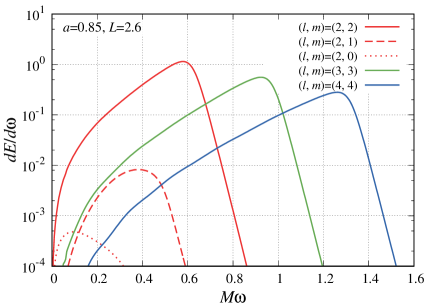
Figure 1: Energy spectrum radiated to infinity in the case of a corotating orbit with $a=0.85M$ and $L=2.6M$.

Next we compute the energies both radiated to the infinity and absorbed by the black hole with ordinary boundary conditions for several sets of the parameters $(a,L)$. In Fig.2, we show both the energy spectra of the $(l,m)=(2,2)$ mode for $a=\{0.1,0.3,0.5,0.7\}M$ and $L=\{0.1,0.5,0.9\}L_{c}^{+}$, where $L_{c}^{\pm}$ is the critical value of the angular momentum

$$L_{c}^{\pm}=\pm 2M(1+\sqrt{1\mp a/M}).$$

In the above equation, the upper sign corresponds to corotating orbits and the lower to counterrotating ones. Our focus is on plunge orbits, and hence we only discuss $L$ that satisfies $L_{c}^{-}<L<L_{c}^{+}$.

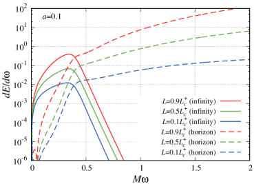
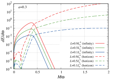
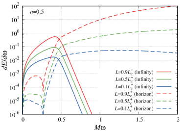
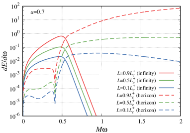
Figure 2: Energy spectra of GWs radiated to infinity and to the horizon of $(l,m)=(2,2)$ for several sets of parameters, $(a,L)$. We choose four values of the Kerr parameter, $a=0.1$ (top left), $a=0.3$ (top right), $a=0.5$ (bottom left), and $a=0.7$ (bottom right). The solid and dashed curves in each panel show the energy spectra to infinity and to the horizon, respectively. Three lines correspond to different values of the angular momentum, $L=0.9L_{c}^{+}$ (red), $L=0.5L_{c}^{+}$ (green), and $L=0.1L_{c}^{+}$ (blue) from top to bottom.

The energy spectra of GWs absorbed by the horizon is largely suppressed at low frequencies. This result turns out to be consistent with the feature of the waveform model proposed in our previous work Uchikata:2019frs ; Nakano:2017fvh . However, the spectra emitted to infinity and to the horizon are not similar at all. The suppression at low frequencies suggested in Ref.Nakano:2017fvh is the one caused by the small transmission coefficient due to the angular momentum barrier, while in the present model the original amplitude of GWs to be reflected by the hypothetical boundary near the horizon is already suppressed at low frequencies. This lack of similarity means that it cannot be an optimal choice to use the waveform of GWs directly emitted to infinity as the seed to generate the echo template.

We can also find that the energy spectrum to the horizon is dominated by the higher frequency band than the quasi-normal mode (QNM) frequency. Here, we consider GWs excited by an in-falling point mass. If we replace the source with a finite size body, there might arise some suppression at high frequencies for ingoing waves falling into the black hole. To suppress the influence of the high frequency modes, which might be an artifact of using the point particle model, it might be appropriate to reduce the amplitude of the high frequency component contained in the waves reflected by the hypothetical boundary near the horizon.

There is also another motivation to introduce a cutoff to the high frequency modes, related to the expected property of the hypothetical reflective boundary near the horizon. There are some proposals suggesting that only low frequency gravitational waves are reflected back by the boundary Bekenstein:1995ju ; Wang:2019rcf ; Oshita:2019sat . In Ref. Bekenstein:1995ju actually proposed was the discretization of the horizon area, from which we naively expect the avoidance of the absorption of low frequency GWs since the state after the absorption is absent. References Wang:2019rcf ; Oshita:2019sat proposed very different independent arguments that suggest the reflective boundary selective to low frequency GWs. To take into account such a possibly expected property of the boundary, here we consider a few simple models that give a frequency dependence to the reflectance of the boundary near the horizon. The simplest one is the sharp cut-off model, given by

$${\rm R}_{b}=\left\{\begin{array}[]{ll}1&(|\omega|<\omega_{c})\\ 0&\mbox{(otherwise)}\end{array}\right.,$$ (84)

where $\omega_{c}>0$ is a parameter introduced as the cutoff frequency. We also introduce a model with the reflectance,

$${\rm R}_{b}=\exp\left[-\left(\frac{\omega-\omega_{{\rm QNM}}}{\sigma_{\omega}}\right)^{2}\right],$$ (85)

where $\omega_{{\rm QNM}}$ is the frequency of the least damped quasi-normal mode for the $m=2$ mode in Kerr spacetime (here we use the fitting function given inBerti:2005ys ), and $\sigma_{\omega}$ is a free parameter. We refer to this model as the Gauusian model. In addition, we consider a reflectance model proposed in Ref. Wang:2019rcf ; Oshita:2019sat ,

$${\rm R}_{b}=e^{-|k|/T_{H}},$$ (86)

where $T_{H}:=(r_{+}^{2}-a^{2})/(4\pi r_{+}(r_{+}^{2}+a^{2}))$ is the Hawking temperature. We refer to this model as the quantum black hole (QBH) model.

In Fig.3, we show the transfer function $|(\epsilon_{\infty,+}/\epsilon_{H,-})\cal K|$ with the various choices of the reflectance on the inner boundary, for $(l,m)=(2,2)$ and $a=0.7$. The factor $|(\epsilon_{\infty,+}/\epsilon_{H,-})|$ is multiplied so that the plot shows the square root of the ratio of the energy flux that reaches the infinity compared with that falls into the black hole in the case without the reflective boundary. We fix the position of the boundary surface at $r_{*b}=-100M$ for all cases.

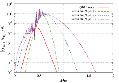
Figure 3: Transfer functions with the reflective surface near the horizon, $(\epsilon_{\infty,+}/\epsilon_{H,-})|\cal K|$. Here we plot the cases with the reflectance of Eq. (84) with the cutoff parameter $\omega_{c}={0.6,0.8,1,2}$ on the left panel, while the cases with those of Eqs. (85) with $\sigma_{\omega}=(0.1,0.2,0.3)$ and (86) on the right panel. We fix $(l,m)=(2,2)$, $a=0.7$ and $r_{*b}=-100M$ for all cases.

Once we obtain $Z^{H}$ under the ordinary boundary conditions and transfer function ${\cal K}$, we can construct the echo amplitude and its waveform measured at infinity under the presence of the reflective boundary near the horizon, through Eq. (72).

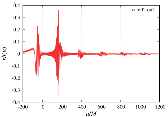
Figure 4: Waveform of the $(l,m)=(2,2)$ mode for the cutoff model with $\omega_{c}=1$. Here we set $(a,L)=(0.7,0.9L_{c}^{+})$ and $r_{*b}=-100M$.

3.2 Comparison with the waveform constructed from the outgoing wave

The time domain waveform observed at infinity can be constructed from the asymptotic form of the Teukolsky variable, $R=Zr^{3}e^{i\omega r_{*}}$ by

$$h(u)=\int d\omega e^{-i\omega u}H(\omega;Z),\quad H(\omega;Z)=-\frac{2}{r}\sum_{lm}\frac{Z}{\omega^{2}}\frac{e^{im\varphi}}{\sqrt{2\pi}}{\rm S}(\theta)$$ (87)

with $u=t-r_{*}$. From Eq. (72), the waveform in the reflective boundary case, $\hat{h}^{\infty}(u)$ is given by

$$\hat{h}^{\infty}(u)=h^{\infty}(u)+h_{{\rm echo}}(u),$$ (88)

where

$$h^{\infty}(u) = \int d\omega e^{-i\omega u}H(\omega;Z^{\infty})\,,$$ (89)

correspond to the waveform observed at infinity in the ordinary BH boundary case, and

$$h_{{\rm echo}}(u) = \int d\omega e^{-i\omega u}H(\omega;{\cal K}Z^{H}),$$ (90)

is that of the series of echoes in the reflective boundary case. As a demonstration, we give the time-domain waveform of the $(l,m)=(2,2)$ mode for the cutoff model with $\omega_{c}=1$ in Fig. 4. Even with the high-frequency cutoff, one can recognize that the first echo is very loud.

In our previous work, we constructed the waveform of echoes using the merger-ringdown waveform observed at infinity as the seed, instead of the waveform of GWs falling into the black hole. Namely, in the present context our previous waveform would correspond to the one obtained by replacing $Z^{H}$ in Eq. (90) with $Z^{\infty}$,

$$\bar{h}_{{\rm echo}}(u)=\int d\omega e^{-i\omega u}H(\omega;{\cal K}Z^{\infty})\,.$$ (91)

To compare $h_{{\rm echo}}$ and $\bar{h}_{{\rm echo}}$, we introduce the overlap between two waveforms by

$$\rho = \max_{\Delta t,\Delta\phi,\bar{r}_{*0}}\frac{(h_{{\rm echo}}|\bar{h}_{{\rm echo}})}{\sqrt{(h_{{\rm echo}}|h_{{\rm echo}})}\sqrt{(\bar{h}_{{\rm echo}}|\bar{h}_{{\rm echo}})}},$$ (92)

with

$$(f|g) \equiv \frac{1}{2\pi}\int_{-\infty}^{\infty}\left[F(\omega)G^{*}(\omega)+F^{*}(\omega)G(\omega)\right]d\omega,$$

where $\Delta t$, $\Delta\phi$ are the shifts of time and phase between the two waveforms, and $\bar{r}_{*b}$, which is the location of the reflective boundary surface for $\bar{h}_{{\rm echo}}$, controls the time interval between neighboring echoes. Here, we assume white noise spectrum, which would be a good approximation as long as we are interested in the waveform whose power is localized in a narrow frequency band. In the above equation, we marginalize $\Delta t$, $\Delta\phi$ and $\bar{r}_{*b}$ in $\bar{h}_{{\rm echo}}$ to maximize $\rho$, while we fix the other parameters to the same values as $h_{{\rm echo}}$. We also define a new estimator for the detectability of the signal when we use a specified echo template, effective filtered amplitude (EFA), by

$${\rm EFA}=\max_{\Delta t,\Delta\phi,\bar{r}_{*b}}\frac{(h_{{\rm echo}}|\bar{h}_{{\rm echo}})}{\sqrt{(h^{\infty}|h^{\infty})}\sqrt{(\bar{h}_{{\rm echo}}|\bar{h}_{{\rm echo}})}}.$$ (93)

This value roughly estimates the amplitude of the echo signal when we project the data by using the template $\bar{h}_{\rm echo}$ relative to the amplitude of $h^{\infty}$. In Table 1 we show the values of $\rho$ and EFA for each model with $a=0.7$, $L=0.9L_{c}^{+}$ and $r_{*b}=-100M$. When $\omega_{c}$ in the cutoff model gets large, the overlap decreases because the fraction of the high frequency modes in $h_{{\rm echo}}$, which is not included in $\bar{h}_{{\rm echo}}$, increases. On the other hand, the EFA gets smaller with the decrease of $\omega_{c}$ because setting $\omega_{c}$ smaller simply reduce the signal contained in the data. A similar behavior of $\rho$ and EFA can be found in the Gaussian models. The EFA for the QBH model is very small compared to the other cases because the amplitude of the echoes is largely suppressed by the transfer function as shown in the right panel of Fig. 3.

model	$\rho$	EFA	$\rho^{\prime}$	$\mbox{EFA}^{\prime}$	$\gamma$
(cutoff)
$\omega_{c}=0.6$	$0.903$	$0.347$	$0.291$	$0.112$	$0.72$
	$(0.895)$	$(0.217)$	$(0.140)$	$(0.0340)$	$(0.51)$
$\omega_{c}=0.8$	$0.673$	$0.588$	$0.162$	$0.142$	$0.62$
	$(0.727)$	$(0.265)$	$(0.105)$	$(0.0385)$	$(0.52)$
$\omega_{c}=1$	$0.443$	$0.623$	$0.101$	$0.142$	$0.63$
	$(0.618)$	$(0.270)$	$(0.0885)$	$(0.0386)$	$(0.51)$
$\omega_{c}=2$	$0.144$	$0.627$	$0.0327$	$0.142$	$0.63$
	$(0.493)$	$(0.270)$	$(0.0705)$	$(0.0386)$	$(0.51)$
(Gaussian)
$\sigma_{\omega}=0.1$	$0.945$	$0.329$	$0.303$	$0.105$	$0.60$
	$(0.951)$	$(0.150)$	$(0.129)$	$(0.0203)$	$(0.53)$
$\sigma_{\omega}=0.2$	$0.839$	$0.445$	$0.245$	$0.130$	$0.63$
	$(0.884)$	$(0.198)$	$(0.111)$	$(0.0249)$	$(0.50)$
$\sigma_{\omega}=0.3$	$0.724$	$0.508$	$0.195$	$0.137$	$0.63$
	$(0.824)$	$(0.223)$	$(0.0977)$	$(0.0264)$	$(0.49)$
QBH	$0.962$	$0.00554$	$0.537$	$0.00309$	$0.13$
	$(0.944)$	$(0.00263)$	$(0.248)$	$(0.000691)$	$(0.12)$

Table 1: Overlap and EFA between two waveforms of echoes for $(l,m)=(2,2)$. The values are computed for $(a,L)=(0.7,0.9L_{c}^{+})$ and $r_{*b}=-100M$. The corresponding values for $L=0.1L_{c}^{+}$ are shown in parentheses for comparison.

Next we evaluate the decline rates of the echoes. The echo term ${{\cal K}}Z^{H}$ in Eq. (72) is composed of the sum of the contributions from individual echoes, which correspond to the respective terms in the series expansion of the transfer function,

$${{\cal K}}Z^{H}=\sum_{n=1}^{\infty}{{\cal K}}^{(n)}Z^{H},\quad{{\cal K}}^{(n)}\equiv({\rm R}_{b}\Phi\hat{r})^{n-1}({\rm R}_{b}\Phi\hat{t})\frac{\Gamma^{\infty,+}}{\Gamma^{H,-}}\,.$$ (94)

Namely, ${{\cal K}}^{(n)}Z^{H}$ corresponds to the amplitude of the $n$-th echo. From this, the whole echo waveform is expressed by a simple additive sum of the waveforms of the individual echoes as

$$h_{{\rm echo}}=\sum_{n=1}^{\infty}h_{{\rm echo}}^{(n)},\quad h_{{\rm echo}}^{(n)}=\int d\omega e^{-i\omega u}H(\omega;{{\cal K}}^{(n)}Z^{H})$$ (95)

In Fig. 5 we show $|H(\omega;{\cal K}^{(n)}Z^{H})|$, the absolute values of the waveform of the $n$-th echo for two representative models. The left panel is the plot for the cutoff model given in Eq. (84) with $\omega_{c}=1$, while the right panel for the QBH model given in Eq. (86). The cutoff model is identical to the case of the perfectly reflective boundary for $M\omega<1$. The first echo contains a large amplitude of high frequency modes, but they disappear in the second and later echoes since the reflectance due to the angular momentum barrier, $\hat{r}$, is almost zero. We also present the case of QBH, because the relative amplitude below the threshold frequency of the super-radiance instability is significantly larger in the late-time echoes than the other cases. Of course, this is not because the lower frequency modes are enhanced but because the higher frequency modes are largely suppressed in the QBH model.

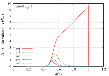
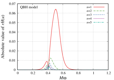
Figure 5: Plots of the absolute values of $H(\omega;{\cal K}^{(n)}Z^{H})$ for $(l,m)=(2,2)$. The left panel is the plot for the cutoff model (84) with $\omega_{c}=1$, while the right panel for the QBH model (86).

In Fig. 6 we also plot $|H(\omega;{\cal K}^{(n)}Z^{\infty})|$, the absolute values of the waveform of the $n$-th echo generated by using $Z^{\infty}$ as the seed, instead of $Z^{H}$. The left panel is the plot for the cutoff model with $\omega_{c}=1$, while the right panel for the QBH model.

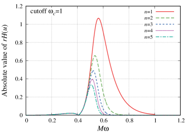
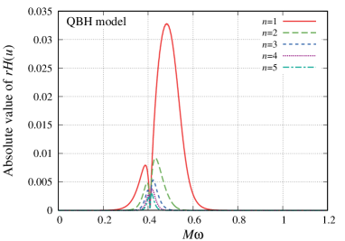
Figure 6: Plots of the absolute values of $H(\omega;{\cal K}^{(n)}Z^{\infty})$ for $(l,m)=(2,2)$. The left panel is for the cutoff model in Eq. (84) with $\omega_{c}=1$, the right panel for the QBH model in Eq. (86).

With the identification of the waveform of each echo mentioned above, we define the following quantities

$$A_{n}\equiv\frac{(h_{{\rm echo}}^{(n)}|h_{{\rm echo}}^{(n)})}{(h_{{\rm echo}}|h_{{\rm echo}})}\,,\quad B_{n}\equiv\frac{(h_{{\rm echo}}^{(n)}|\bar{h}^{(n)}_{{\rm echo}})}{\sqrt{(h_{{\rm echo}}|h_{{\rm echo}})}\sqrt{(\bar{h}_{{\rm echo}}|\bar{h}_{{\rm echo}})}}\,,$$ (96)

where $B_{n}$ is evaluated with the same common values of $\Delta t$, $\Delta\phi$ and $\bar{r}_{*b}$ as those used in the maximization in Eq. (92). $A_{n}$ is the relative amplitude of each echo to the total echoes, and $B_{n}$ is the relative overlap between the $n$-th echo component of $h_{{\rm echo}}$ and that of $\bar{h}_{{\rm echo}}$.

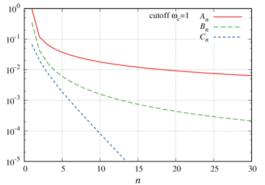
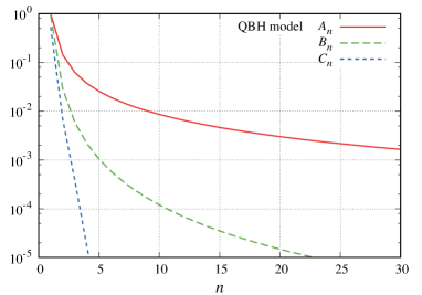
Figure 7: Plots of $A_{n}$, $B_{n}$ and $C_{n}$ for $(l,m)=(2,2)$. The left panel is the plot for the cutoff model (84) with $\omega_{c}=1$, and the right panel for the QNM model (86). Here we fix $(a,L)=(0.7,0.9L_{c}^{+})$ and $r_{*b}=-100M$.

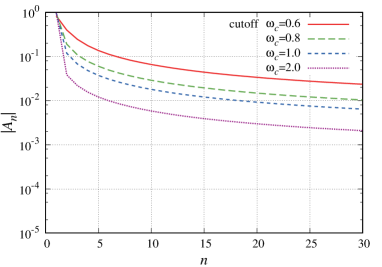
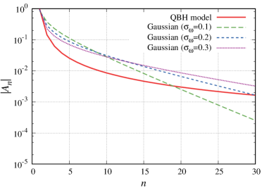
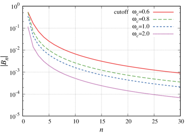
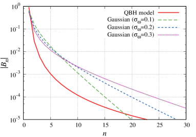
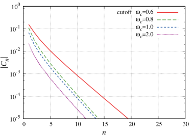
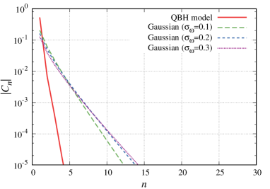
Figure 8: Comparison of $A_{n}$, $B_{n}$ and $C_{n}$ for several models. The left panels are the plots for the cutoff models while the right panels for the Gaussian models and the QBH model. Here we fix $(a,L)=(0.7,0.9L_{c}^{+})$ and $r_{*b}=-100M$.

For comparison, we also consider an even simpler waveform model of echoes:

$$\bar{h}^{\prime}_{{\rm echo}}(u)=\sum_{n=1}^{\infty}\bar{h}^{\prime(n)}_{{\rm echo}}(u),\quad\bar{h}^{\prime(n)}_{{\rm echo}}(u)=(-1)^{n}\gamma^{n-1}h^{\infty}(u-(n-1)\Delta t_{{\rm echo}}),$$ (97)

where $\gamma$ and $\Delta t_{{\rm echo}}$, independent of the frequency, are corresponding to the damping factor and the time interval between successive echoes used in the analysis in Ref. Abedi:2016hgu . This model just repeats exactly the same waveform with a minus sign, periodically with decaying amplitude. We define the overlap and EFA between $h_{{\rm echo}}$ and $\bar{h}^{\prime}_{{\rm echo}}$ as

$$\rho^{\prime} = \max_{\Delta t^{\prime},\Delta\phi^{\prime},\gamma,\Delta t_{{\rm echo}}}\frac{(h_{{\rm echo}}|\bar{h}^{\prime}_{{\rm echo}})}{\sqrt{(h_{{\rm echo}}|h_{{\rm echo}})}\sqrt{(\bar{h}^{\prime}_{{\rm echo}}|\bar{h}^{\prime}_{{\rm echo}})}}\,,$$ (98)

$${\rm EFA}^{\prime} = \max_{\Delta t^{\prime},\Delta\phi^{\prime},\gamma,\Delta t_{{\rm echo}}}\frac{(h_{{\rm echo}}|\bar{h}^{\prime}_{{\rm echo}})}{\sqrt{(h^{\infty}|h^{\infty})}\sqrt{(\bar{h}^{\prime}_{{\rm echo}}|\bar{h}^{\prime}_{{\rm echo}})}}\,,$$ (99)

where we marginalize $\Delta t^{\prime}$, $\Delta\phi^{\prime}$, $\gamma$ and $\Delta t_{{\rm echo}}$ to maximize $\rho^{\prime}$ and ${\rm EFA}^{\prime}$. In Table 1, we show the values of $\rho^{\prime}$, ${\rm EFA}^{\prime}$ and $\gamma$ for the maximization. Both $\rho^{\prime}$ and ${\rm EFA}^{\prime}$ are significantly smaller than $\rho$ and EFA. This means that the template proposed in Ref. Nakano:2017fvh better captures the feature of the echo signal expected by the model with a reflective boundary near the horizon. At the same time we find that the best fit value for the decay rate $\gamma$ is not so large. This is not consistent with the results of the data analysis presented in Ref. Abedi:2016hgu .

In a similar manner to $B_{n}$, we also define

$$C_{n}\equiv\frac{(h_{{\rm echo}}^{(n)}|\bar{h}^{\prime(n)}_{{\rm echo}})}{\sqrt{(h_{{\rm echo}}|h_{{\rm echo}})}\sqrt{(\bar{h}^{\prime}_{{\rm echo}}|\bar{h}^{\prime}_{{\rm echo}})}}\,.$$ (100)

In Figs. 7 and 8, we show the plots of $A_{n}$, $B_{n}$ and $C_{n}$ as functions of $n$ for a representative case with $a=0.7$ and $L=0.9L_{c}^{+}$. $B_{n}$ is much smaller than $A_{n}$, which means that the echo waveform by using GWs emitted to infinity as the seed is not really a good approximation. Nevertheless, $B_{n}$ decreases much less rapidly than $C_{n}$.

In Fig. 8, we give a comparison of $A_{n}$, $B_{n}$ and $C_{n}$ for several models. Here, we adopt $(a,L)=(0.7,0.9L_{c}^{+})$ as the representative values. The left panels are the plots for the cutoff models. All the cases behave very similarly, i.e., the higher cutoff frequency leads to the smaller magnitude for the second and later echoes because the higher frequency modes, which are contained only in the first echo waveform, are emphasized. In the right panels we give the plots for the Gaussian models and the QBH model. These plots show that the Gaussian model with broader frequency band decays more rapidly at the beginning but more slowly at a late time. This is because the model contains both the rapidly escaping high frequency modes and the long-lasting low frequency modes.

4 Conclusion

We have investigated the expected feature of the waveform of GW echoes in the model with a hypothetical reflective boundary near the horizon. As a model which is easy to handle, we consider perturbations induced by a particle falling into a Kerr black hole, instead of a binary coalescence. In the latter case, it is not so clear how to impose the modified reflective boundary condition near the horizon of the black hole newly formed after the merger. By contrast, imposing the reflective boundary condition at the boundary is mathematically well-posed in the case of black hole perturbation.

We used the Sasaki-Nakamura equation to calculate GWs induced by a point mass falling into a Kerr black hole. We clarified the method how to compute GWs absorbed by the black hole by using the Sasaki-Nakamura equation, and developed a prescription to impose the reflective boundary condition near the horizon. For simplicity, our computation was restricted to the case in which the point mass is in an equatorial orbit and initially at rest at $r=\infty$, but its angular momentum was varied. Independently of whether the angular momentum is small or large, the obtained spectrum of GWs absorbed by the black hole is dominated by modes with a higher frequency than that of the fundamental quasi-normal mode. As a result, the echo signal obtained by introducing a reflective boundary near the horizon is also dominated by high frequency modes.

If we assume that the echo waveform is given by a simple repetition of the waveform of GWs emitted to infinity, a significantly large fraction of echo signal is contained in the frequency band lower than the QNM frequency. However, our analysis suggests that a simple reflective boundary model will not predict large power in echoes at such low frequencies.

In Ref. Uchikata:2019frs we reanalyzed LIGO data searching for the echo signal after binary black hole merger. However, the use of our templates that take into account the reflection rate of the angular momentum barrier did not improve the significance of the signal suggested in Ref. Abedi:2016hgu . The main difference in the templates used in these two analyses is in the low frequency bands. If there exists echo signal dominated by lower frequency modes, our analysis presented in this paper suggests that we need to consider more complicated model than the model with a simple reflective boundary near the horizon.

References

- (1) B. P. Abbott et al. [LIGO Scientific and Virgo], Phys. Rev. Lett. 116 (2016) no.6, 061102 doi:10.1103/PhysRevLett.116.061102 [arXiv:1602.03837 [gr-qc]].
- (2) B. P. Abbott et al. [LIGO Scientific and Virgo Collaborations], Phys. Rev. D 93, 122003 (2016) [arXiv:1602.03839 [gr-qc]].
- (3) B. P. Abbott et al. [LIGO Scientific and Virgo], Phys. Rev. X 9 (2019) no.3, 031040 doi:10.1103/PhysRevX.9.031040 [arXiv:1811.12907 [astro-ph.HE]].
- (4) LIGO Scientific Collaboration and Virgo Collaboration, ”GWTC-1 Documentation” on GW Open Science Center, https://doi.org/10.7935/82H3-HH23 (2018).
- (5) J. Abedi, H. Dykaar and N. Afshordi, arXiv:1612.00266 [gr-qc].
- (6) G. Ashton et al., arXiv:1612.05625 [gr-qc].
- (7) J. Abedi, H. Dykaar and N. Afshordi, arXiv:1701.03485 [gr-qc].
- (8) J. Westerweck, A. Nielsen, O. Fischer-Birnholtz, M. Cabero, C. Capano, T. Dent, B. Krishnan, G. Meadors and A. H. Nitz, Phys. Rev. D 97 (2018) no.12, 124037 doi:10.1103/PhysRevD.97.124037 [arXiv:1712.09966 [gr-qc]].
- (9) A. B. Nielsen, C. D. Capano, O. Birnholtz and J. Westerweck, Phys. Rev. D 99 (2019) no.10, 104012 doi:10.1103/PhysRevD.99.104012 [arXiv:1811.04904 [gr-qc]].
- (10) R. K. L. Lo, T. G. F. Li and A. J. Weinstein, Phys. Rev. D 99 (2019) no.8, 084052 doi:10.1103/PhysRevD.99.084052 [arXiv:1811.07431 [gr-qc]].
- (11) N. Uchikata, H. Nakano, T. Narikawa, N. Sago, H. Tagoshi and T. Tanaka, Phys. Rev. D 100 (2019) no.6, 062006 doi:10.1103/PhysRevD.100.062006 [arXiv:1906.00838 [gr-qc]].
- (12) J. Abedi and N. Afshordi, [arXiv:2001.00821 [gr-qc]].
- (13) V. Cardoso, E. Franzin and P. Pani, Phys. Rev. Lett. 116 (2016) no.17, 171101 doi:10.1103/PhysRevLett.116.171101 [arXiv:1602.07309 [gr-qc]].
- (14) V. Cardoso, S. Hopper, C. F. B. Macedo, C. Palenzuela and P. Pani, Phys. Rev. D 94 (2016) no.8, 084031 doi:10.1103/PhysRevD.94.084031 [arXiv:1608.08637 [gr-qc]].
- (15) P. O. Mazur and E. Mottola, Proc. Nat. Acad. Sci. 101 (2004), 9545-9550 doi:10.1073/pnas.0402717101 [arXiv:gr-qc/0407075 [gr-qc]].
- (16) Visser M (1995) Lorentzian wormholes: from Einstein to Hawking. AIP Press/Springer, Woodbury.
- (17) T. Damour and S. N. Solodukhin, Phys. Rev. D 76 (2007), 024016 doi:10.1103/PhysRevD.76.024016 [arXiv:0704.2667 [gr-qc]].
- (18) A. Almheiri, D. Marolf, J. Polchinski and J. Sully, JHEP 02 (2013), 062 doi:10.1007/JHEP02(2013)062 [arXiv:1207.3123 [hep-th]].
- (19) V. Cardoso and P. Pani, Living Rev. Rel. 22 (2019) no.1, 4 doi:10.1007/s41114-019-0020-4 [arXiv:1904.05363 [gr-qc]].
- (20) H. Nakano, N. Sago, H. Tagoshi and T. Tanaka, PTEP 2017 (2017) no.7, 071E01 doi:10.1093/ptep/ptx093 [arXiv:1704.07175 [gr-qc]].
- (21) Z. Mark, A. Zimmerman, S. M. Du and Y. Chen, Phys. Rev. D 96 (2017) no.8, 084002 doi:10.1103/PhysRevD.96.084002 [arXiv:1706.06155 [gr-qc]].
- (22) C. P. Burgess, R. Plestid and M. Rummel, JHEP 09 (2018), 113 doi:10.1007/JHEP09(2018)113 [arXiv:1808.00847 [gr-qc]].
- (23) R. S. Conklin and B. Holdom, Phys. Rev. D 100 (2019) no.12, 124030 doi:10.1103/PhysRevD.100.124030 [arXiv:1905.09370 [gr-qc]].
- (24) E. Maggio, A. Testa, S. Bhagwat and P. Pani, Phys. Rev. D 100 (2019) no.6, 064056 doi:10.1103/PhysRevD.100.064056 [arXiv:1907.03091 [gr-qc]].
- (25) L. F. L. Micchi and C. Chirenti, Phys. Rev. D 101 (2020) no.8, 084010 doi:10.1103/PhysRevD.101.084010 [arXiv:1912.05419 [gr-qc]].
- (26) G. D’Amico and N. Kaloper, Phys. Rev. D 102 (2020) no.4, 044001 doi:10.1103/PhysRevD.102.044001 [arXiv:1912.05584 [gr-qc]].
- (27) S. A. Teukolsky, Astrophys. J. 185, 635 (1973).
- (28) W. H. Press and S. A. Teukolsky, Astrophys. J. 185, 649 (1973).
- (29) S. A. Teukolsky and W. H. Press, Astrophys. J. 193 (1974), 443-461 doi:10.1086/153180
- (30) M. Sasaki and T. Nakamura, Phys. Lett. A 89, 68 (1982).
- (31) M. Sasaki and T. Nakamura, Prog. Theor. Phys. 67, 1788 (1982).
- (32) T. Nakamura and M. Sasaki, Phys. Lett. A 89, 185 (1982).
- (33) Y. Kojima and T. Nakamura, Prog. Theor. Phys. 71 (1984), 79-90 doi:10.1143/PTP.71.79
- (34) T. Nakamura, K. Oohara and Y. Kojima, Part III of Prog. Theor. Phys. Suppl. 90 (1987), 1-218 doi:10.1143/PTPS.90.1
- (35) J. D. Bekenstein and V. F. Mukhanov, Phys. Lett. B 360 (1995), 7-12 doi:10.1016/0370-2693(95)01148-J [arXiv:gr-qc/9505012 [gr-qc]].
- (36) Q. Wang, N. Oshita and N. Afshordi, Phys. Rev. D 101 (2020) no.2, 024031 doi:10.1103/PhysRevD.101.024031 [arXiv:1905.00446 [gr-qc]].
- (37) N. Oshita, Q. Wang and N. Afshordi, JCAP 04 (2020), 016 doi:10.1088/1475-7516/2020/04/016 [arXiv:1905.00464 [hep-th]].
- (38) E. Berti, V. Cardoso and C. M. Will, Phys. Rev. D 73 (2006), 064030 doi:10.1103/PhysRevD.73.064030 [arXiv:gr-qc/0512160 [gr-qc]].