On attainability of Kendall’s tau matrices
and concordance signatures

Abstract

Methods are developed for checking and completing systems of bivariate and multivariate Kendall’s tau concordance measures in applications where only partial information about dependencies between variables is available. The concept of a concordance signature of a multivariate continuous distribution is introduced; this is the vector of concordance probabilities for margins of all orders. It is shown that every attainable concordance signature is equal to the concordance signature of a unique mixture of the extremal copulas, that is the copulas with extremal correlation matrices consisting exclusively of $1$’s and $-1$’s. A method of estimating an attainable concordance signature from data is derived and shown to correspond to using standard estimates of Kendall’s tau in the absence of ties. The set of attainable Kendall rank correlation matrices of multivariate continuous distributions is proved to be identical to the set of convex combinations of extremal correlation matrices, a set known as the cut polytope. A methodology for testing the attainability of concordance signatures using linear optimization and convex analysis is provided. The elliptical copulas are shown to yield a strict subset of the attainable concordance signatures as well as a strict subset of the attainable Kendall rank correlation matrices; the Student $t$ copula is seen to converge, as the degrees of freedom tend to zero, to a mixture of extremal copulas sharing its concordance signature with all elliptical distributions that have the same correlation matrix. blackA characterization of the attainable signatures of equiconcordant copulas is given.

Keywords: Attainable correlations; concordance; copulas; cut-polytope; elliptical distributions; extremal distributions; exchangeability; Kendall’s rank correlation; multivariate Bernoulli distributions.

1 Introduction

In many real-world applications of statistics a modeler is required to impute missing information on the dependencies between variables, typically in the form of correlations. This problem is particularly common in finance and insurance where data on certain risks are often sparse or non-existent. Some financial institutions use copulas parameterized in part by expert-elicited correlations to build joint models of key risks affecting their solvency and profitability (Embrechts et al., 2002; Shaw et al., 2011). For example, a large insurer analyzing excess risk due to the Covid-19 pandemic might consider the interplay between mortality risk, business interruption risk, financial investment risk and trade credit insurance risk. While dependencies between these risks may be significant and non-negligible, they are also difficult to quantify. In the related area of asset management a model for the dependencies between asset returns is essential for optimizing a portfolio. However many assets have no track record and plausible values must be entered if they are to be included in the analysis. Assessing dependence in the absence of data is also relevant in causal inference when unmeasured confounders are present (Stokes et al., 2020).

Imputing missing information on dependence is a challenging problem because of the complex relationships between different pairs or subgroups of variables. The general problem of determining the compatibility of lower-dimensional margins of higher-dimensional distributions has only been partially resolved (see Joe, 1996, 1997, among others). In this paper, we investigate the related problem of compatibility of correlation measures for subgroups of variables. Even for the classical linear correlation of Pearson, the set of attainable correlation matrices has not been fully characterized. Because Pearson’s correlation depends on the marginal distributions, the set of attainable matrices is generally much more complicated than the elliptope of positive semi-definite correlation matrices investigated, for example, by Huber and Marić (2015, 2019), unless attention is restricted to special choices of margins such as the normal (Embrechts et al., 2002). Recently, Hofert and Koike (2019) described the set of attainable Blomqvist’s beta matrices, while Embrechts et al. (2016) found conditions characterizing matrices of tail dependence coefficients. Devroye and Letac (2015) and Wang et al. (2019) consider the set of attainable Spearman rank correlation matrices; this coincides with the elliptope of linear $d\times d$ correlation matrices when $d\leqslant 9$ but not when $d\geqslant 12$, while the case where $d\in\{10,11\}$ remains to be settled.

In this paper, we provide a complete solution to the attainability and compatibility problem when dependence is measured by the widely-used Kendall’s tau rank correlation (Kendall, 1938; Kruskal, 1958; Joe, 1990) which parametrizes many popular dependence models. In order to take into account bivariate and higher-order associations between subsets of variables, we quantify the dependence of a multivariate random vector using a vector-valued measure that we call the concordance signature, which underlies all bivariate and multivariate Kendall’s tau coefficients; this concept is made precise in Section 2.

blackA note on our use of the terms attainability and compatibility may be helpful at this point. We use attainable when we talk about a logically coherent collective entity that could belong to a probability distribution, such as a concordance signature or a Kendall’s tau matrix. We use compatible when we talk about the relationship between sub-components of an attainable entity, such as Kendall’s tau rank correlations for different pairs of variables. We also refer to attainable signatures as being compatible with probability distributions.

Our main result is to fully characterize the set of attainable concordance signatures of continuous multivariate distributions. As a by-product, we prove the conjecture of Hofert and Koike (2019) that the set of attainable Kendall rank correlation matrices is identical to the set of convex combinations of the extremal correlation matrices, i.e., the correlation matrices consisting exclusively of $1$’s and $-1$’s; this set is also known as the cut polytope (Laurent and Poljak, 1995). As we show, this characterization follows from the links between concordance signatures, multivariate Bernoulli distributions, and extremal mixture copulas, i.e., mixtures of the $2^{d-1}$ possible copulas with extremal correlation matrices (Tiit, 1996). We explain why the set of attainable Kendall correlation matrices is identical to the set of attainable correlation matrices for multivariate Bernoulli random vectors with symmetric margins as derived by Huber and Marić (2015, 2019).

The methodology we propose has a number of important applications. First, it allows us to determine whether a set of estimated or expert-elicited Kendall correlations (bivariate or multivariate) is compatible with a valid multivariate distribution. If it is, we then propose a method of determining the set in which any remaining unmeasured Kendall correlations must lie using standard techniques from linear optimization and convex analysis. To illustrate, suppose, for example, we have Bitcoin, Etherium and Litecoin in our portfolio and we invest in a new cryptocurrency ‘X4coin’. Based on return data for Bitcoin, Etherium and Litecoin in 2017, the attainable Kendall rank correlations between the as yet unobserved X4coin and the other three currencies can be shown to lie in the three-dimensional polytope in the left panel of Figure 1. As soon as we form an opinion on the rank correlation between X4coin and one of the cryptocurrencies, this further restricts the set of possible rank correlations between X4coin and the other two currencies, as shown in the right panel of Figure 1; full details are given later in Example 3.

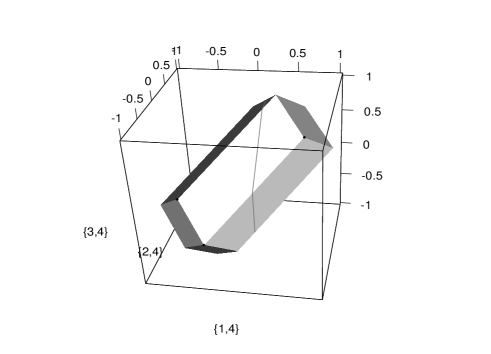
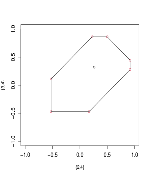
Figure 1: Left panel: set of attainable Kendall rank correlations for X4coin paired with three other cryptocurrencies in Example 3. Right panel: set of attainable Kendall’s tau values for (X4coin, Etherium) and (X4coin, Litecoin) when the (X4coin, Bitcoin) value is fixed at 0.598.

We also prove that sample concordance signatures based on classical estimators of Kendall’s tau are themselves concordance signatures of valid multivariate distributions. Our finding that the concordance signature of a multivariate distribution with continuous margins is always equal to the concordance signature of a unique mixture of the extremal copulas then offers a powerful technique in Monte Carlo simulation or risk analyses. It allows us to draw realizations from a model with identical concordance signature to that estimated from the data but with an extreme form of tail dependence.

Finally, our methodology allows us to take a closer look at the dependence structure inherent in different classes of distributions. We show that the concordance signatures of the family of elliptical copulas form a strict subset of the set of all possible attainable concordance signatures. The surprising consequence is the existence of Kendall correlation matrices that do not correspond to any elliptically distributed random vector; this behavior provides a contrast with Pearson correlation matrices, each of which is the correlation matrix of at least one elliptical distribution. Moreover, we show that the $d$-dimensional Student $t$ copula with correlation matrix $P\in\mathbb{R}^{d\times d}$ and degree-of-freedom parameter $\nu>0$ converges pointwise to a mixture of extremal copulas which shares its concordance signature as $\nu\to 0$. blackWe also investigate the concordance signatures of exchangeable and equiconconcordant distributions.

2 Concordance signatures

Throughout this paper, we use bold symbols such as $\bm{x}=(x_{1},\dots,x_{d})$ to denote vectors in $\mathbb{R}^{d}$ and understand expressions such as $\bm{x}+\bm{y}$ as componentwise operations; similarly $\bm{x}\leqslant\bm{y}$ implies that all components are ordered.

Let $\bm{X}=(X_{1},\ldots,X_{d})$ denote a generic random vector with continuous margins $F_{1},\ldots,F_{d}$. As is well known, the unique copula $C$ of $\bm{X}$ is the distribution function of the random vector $\bm{U}=(U_{1},\ldots,U_{d})$ where $U_{i}=F_{i}(X_{i})$ for $i=1,\ldots,d$ (Joe, 1997; Nelsen, 2006).

For any subset $I\subseteq\mathcal{D}=\{1,\ldots,d\}$ with $I\neq\emptyset$ we write $\bm{X}_{I}$ and $\bm{U}_{I}$ to denote sub-vectors of $\bm{X}$ and $\bm{U}$, and $C_{I}$ for the copula of $\bm{X}_{I}$, i.e., the distribution function of $\bm{U}_{I}$. The multivariate probability of concordance of $\bm{X}_{I}$ is defined as

$$\kappa_{I}=\mathbb{P}\left(\{\bm{X}_{I}\leqslant\bm{X}^{*}_{I}\}\cup\{\bm{X}^{*}_{I}\leqslant\bm{X}_{I}\}\right),$$ (1)

where $\bm{X}^{*}$ is a random vector independent of $\bm{X}$ but with the same distribution. Note that (1) implies $\kappa_{\{i\}}=1$ for a singleton and we adopt the convention $\kappa_{\emptyset}=1$.

For subsets with cardinality $|I|\geqslant 2$, the concordance probabilities quantify the association between the components of $\bm{X}_{I}$. Indeed $\kappa_{I}$ is related to Kendall’s tau $\tau_{I}$ (Kendall, 1938; Kruskal, 1958) when $|I|=2$ and to its multivariate analogue (Joe, 1990; Genest et al., 2011) when $|I|>2$ via the formula

$$(2^{|I|-1}-1)\tau_{I}=2^{|I|-1}\kappa_{I}-1\;.$$ (2)

Moreover, following Nelsen (2006), $\kappa_{I}$ depends only on the copula $C_{I}$ of $\bm{X}_{I}$ according to

$$\kappa_{I}=2\mathbb{P}\left(\bm{X}_{I}\leqslant\bm{X}^{*}_{I}\right)=2\mathbb{P}\left(\bm{U}_{I}\leqslant\bm{U}^{*}_{I}\right)=2\int_{[0,1]^{|I|}}C_{I}(\bm{u})dC_{I}(\bm{u}).$$ (3)

Without loss of generality, we can thus refer to $\kappa_{I}$ as the concordance probability of the copula $C_{I}$ of $\bm{X}_{I}$ and use the notation $\kappa_{I}=\kappa(C_{I})=\kappa(\bm{X}_{I})=\kappa(\bm{U}_{I})$ interchangeably.

To summarize the various dependencies inherent in the vector $\bm{X}$, we can collect the values $\kappa_{I}$ for all subsets $I\in\mathcal{P}(\mathcal{D})$, where $\mathcal{P}(\mathcal{D})$ denotes the power set of $\mathcal{D}$. This motivates calling the vector $(\kappa_{I}:I\in\mathcal{P}(\mathcal{D}))$ the full concordance signature of $\bm{X}$. Sub-vectors of the full concordance signature are known as partial concordance signatures. From Proposition 1 in Genest et al. (2011), which is based on the exclusion-inclusion principle, we can deduce that for any set $I\subseteq\mathcal{D}$ of odd cardinality,

$$\kappa_{I}=1+\sum_{A\subset I,1\leqslant|A|<|I|}(-1)^{|A|}\mathbb{P}(\bm{U}_{A}\leqslant\bm{U}^{*}_{A})=1-\frac{|I|}{2}+\sum_{A\subset I,2\leqslant|A|<|I|}(-1)^{|A|}\frac{\kappa_{A}}{2}\;.$$ (4)

Thus the full concordance signature can be deduced from the concordance probabilities for subsets of $\mathcal{D}$ of even cardinality. We formalize ideas in the following definition.

Definition 1.

A label set is any collection $S$ of subsets of $\mathcal{D}$ such that $\emptyset\in S$. The vector $\bm{\kappa}_{S}(C)=(\kappa(C_{I}):I\in S)$ is called the partial concordance signature of the copula $C$ for the label set $S$. By convention, the elements of $S$ are taken in lexicographical order. When the label set is the even power set $\mathcal{E}(\mathcal{D})=\{I:I\subseteq\mathcal{D},|I|\,\text{even}\}$ (containing the empty set $\emptyset$ by convention) the partial concordance signature is called the even concordance signature of $C$ and is denoted $\bm{\kappa}(C)$. When the label set is $\mathcal{P}(\mathcal{D})$ the partial concordance signature is called the full concordance signature of $C$ and is denoted $\tilde{\bm{\kappa}}(C)$.

3 Extremal mixture copulas

Our main tools for the study of concordance signatures are mixtures of so-called extremal copulas and their relationship with multivariate Bernoulli distributions. In this section we develop the necessary notation and theory.

An extremal copula $C$ with index set $J\subseteq\mathcal{D}$ is the distribution function of the random vector $\bm{U}=(U_{1},\ldots,U_{d})$ where for $j\in\mathcal{D}$, $U_{j}\stackrel{{\scriptstyle\text{\tiny d}}}{{=}}U$ if $j\in J$, $U_{j}\stackrel{{\scriptstyle\text{\tiny d}}}{{=}}1-U$ if $j\in J^{\complement}$, and $U$ is a standard uniform random variable. For all $\bm{u}\in[0,1]^{d}$ it has the explicit form

$$C(\bm{u})=(\min_{j\in J}u_{j}+\min_{j\in J^{\complement}}u_{j}-1)^{+}\;,$$ (5)

where for any $x\in\mathbb{R}$, $x^{+}=\max(x,0)$ denotes the positive part of $x$ and we employ the convention $\min_{j\in\emptyset}u_{j}=1$.

In dimension $d\geqslant 2$ there are $2^{d-1}$ extremal copulas and we enumerate them in the following way. For $k\in\{1,\ldots,2^{d-1}\}$ let $\bm{s}_{k}=(s_{k,1},\ldots,s_{k,d})$ be the vector consisting of the digits of $k-1$ when represented as a $d$-digit binary number. For example, when $d=4$ we have exactly eight extremal copulas corresponding to the vectors

$$\bm{s}_{1} =(0,0,0,0),\quad\bm{s}_{2}=(0,0,0,1),\quad\bm{s}_{3}=(0,0,1,0),\quad\bm{s}_{4}=(0,0,1,1),$$

$$\bm{s}_{5} =(0,1,0,0),\quad\bm{s}_{6}=(0,1,0,1),\quad\bm{s}_{7}=(0,1,1,0),\quad\bm{s}_{8}=(0,1,1,1).$$

For each $k\in\{1,\ldots,2^{d-1}\}$, $\bm{s}_{k}=(s_{k,1},\ldots,s_{k,d})$ and $\bm{1}-\bm{s}_{k}=(1-s_{k,1},\ldots,1-s_{k,d})$ are opposite vertices of the unit hypercube connected by one of its $2^{d-1}$ main diagonals, $\bm{1}$ being the vector of ones. The $k$th extremal copula in dimension $d$, denoted $C^{(k)}$, spreads its probability mass uniformly along the latter diagonal joining $\bm{s}_{k}$ and $\bm{1}-\bm{s}_{k}$. Its index set $J_{k}\subseteq\mathcal{D}=\{1,\ldots,d\}$ is defined as the set of indices corresponding to zeros in $\bm{s}_{k}$; that is, $j\in J_{k}$ if $s_{k,j}=0$ and $j\in J_{k}^{\complement}$ if $s_{k,j}=1$. For the 4-dimensional example above we have $J_{1}=\{1,2,3,4\}$, $J_{1}^{\complement}=\emptyset$, $J_{2}=\{1,2,3\}$, $J_{2}^{\complement}=\{4\}$ and so on. Note also that $J_{1}=\mathcal{D}$ so that $C^{(1)}(\bm{u})=\min(u_{1},\ldots,u_{d})$ is the comonotonicity or Fréchet–Hoeffding upper bound copula.

Extremal copulas owe their name to the fact that their correlation matrices are extremal correlation matrices, that is, matrices consisting exclusively of 1’s and $-1$’s. Indeed, for any $k\in\{1,\ldots,2^{d-1}\}$, we find that the matrix of pairwise Kendall’s tau values for the $k$th extremal copula $C^{(k)}$ is $P^{(k)}=(2\bm{s}_{k}-\bm{1})(2\bm{s}_{k}-\bm{1})^{\top}$. This matrix is simultaneously the matrix of pairwise Pearson and Spearman correlations of $C^{(k)}$.

Definition 2.

An extremal mixture copula is a copula of the form $C^{*}=\sum_{k=1}^{2^{d-1}}w_{k}C^{(k)}$, where for all $k\in\{1,\ldots,2^{d-1}\}$, $C^{(k)}$ is the $k$th extremal copula, $w_{k}\geqslant 0$, and $\sum_{k=1}^{2^{d-1}}w_{k}=1$.

The following proposition shows how the extremal mixture copulas are related to multivariate Bernoulli distributions; the proof is given in A.

Proposition 1.

Let $U$ be a standard uniform random variable and $\boldsymbol{B}$ a $d$-dimensional multivariate Bernoulli vector independent of $U$. Then the distribution function of the vector

$$U\boldsymbol{B}+(1-U)(\boldsymbol{1}-\boldsymbol{B})$$ (6)

is an extremal mixture with weights given, for each $k\in\{1,\ldots,2^{d-1}\}$, by

$$w_{k}=\mathbb{P}(\boldsymbol{B}=\boldsymbol{s}_{k})+\mathbb{P}(\boldsymbol{B}=\bm{1}-\boldsymbol{s}_{k}),$$ (7)

where $\boldsymbol{s}_{k}$ is the vector consisting of the digits of $k-1$ when represented as a $d$-digit binary number. Conversely, any extremal mixture copula $C^{*}=\sum_{k=1}^{2^{d-1}}w_{k}C^{(k)}$ is the distribution function of a random vector of the form (6), where $U$ is independent of $\boldsymbol{B}$ and (7) holds for all $k\in\{1,\ldots,2^{d-1}\}$.

The class of Bernoulli distributions satisfying (7) is infinite since the mass $w_{k}$ can be split between the events $\{\boldsymbol{B}=\boldsymbol{s}_{k}\}$ and $\{\boldsymbol{B}=\bm{1}-\boldsymbol{s}_{k}\}$ in an arbitrary way. It is important for the arguments used in this paper to single out a representative and we do this by setting $\boldsymbol{B}=\boldsymbol{Y}$, where $\boldsymbol{Y}$ is radially symmetric about $\boldsymbol{0.5}$. This means that $\bm{Y}\stackrel{{\scriptstyle d}}{{=}}\bm{1}-\bm{Y}$ and implies that, for each $k\in\{1,\ldots,2^{d-1}\}$,

$$\mathbb{P}(\boldsymbol{Y}=\boldsymbol{s}_{k})=\mathbb{P}(\boldsymbol{Y}=\boldsymbol{1}-\boldsymbol{s}_{k})=0.5w_{k}.$$ (8)

Such distributions are also known as palindromic Bernoulli distributions (Marchetti and Wermuth, 2016) and they are fully parameterized by the $2^{d-1}$ probabilities $\mathbb{P}(\bm{Y}=\bm{s}_{k})=0.5w_{k}$, $k\in\{1,\ldots,2^{d-1}\}$. This means that there is a bijective mapping between the extremal mixture copulas and the radially symmetric multivariate Bernoulli distributions in dimension $d$. A number of constraints apply to radially symmetric Bernoulli random vectors. Apart from the fact that $\mathbb{P}(Y_{i}=1)=0.5$ for all $i$, we will make use of the following insight, proved in A.

Proposition 2.

1. The radially symmetric Bernoulli distribution of a vector $\bm{Y}$ in dimension $d$ is uniquely determined by the vector of probabilities $\bm{p}_{\bm{Y}}=(p_{I}:I\in\mathcal{E}(\mathcal{D})\setminus\emptyset)$, where $p_{I}=\mathbb{P}(\bm{Y}_{I}=\bm{1})$ and $\mathcal{E}(\mathcal{D})$ is the even power set as in Definition 1.

2. The vector $\bm{p}_{\bm{Y}}$ in (i) is the shortest vector of the form $(p_{I}:I\in S\setminus\emptyset)$ for a label set $S\subset\mathcal{P}(\mathcal{D})$ which uniquely determines the distribution of $\bm{Y}$ for all blackradially symmetric Bernoulli random vectors $\bm{Y}$.

We close this section by noting that the independence between $U$ and $\boldsymbol{Y}$ in the stochastic representation $\bm{U}\stackrel{{\scriptstyle\text{\tiny d}}}{{=}}U\bm{Y}+(1-U)(\bm{1}-\bm{Y})$ of an extremal mixture copula cannot be dispensed with. An example of a copula that violates this condition is provided in A and reveals an interesting contrast between the extremal copulas and the mixtures of extremal copulas. While a necessary and sufficient condition for a vector $\bm{U}$ to be distributed according to an extremal copula is that its bivariate margins should be extremal copulas (Tiit, 1996), the analogous statement does not hold for extremal mixture copulas. Although it is necessary that the bivariate margins of an extremal mixture copula are extremal mixture copulas, the example shows that this is not sufficient. An additional condition is required, as detailed in the next proposition which is proved in A.

Proposition 3.

The distribution of a random vector $\bm{U}=(U_{1},\ldots,U_{d})$ is a mixture of extremal copulas if and only if its bivariate marginal distributions are mixtures of extremal copulas and for all $u\in[0,1]$,

$$\mathbb{P}\left(U_{1}\leqslant u\mid\mathbbm{1}_{\{U_{j}=U_{1}\}},j\neq 1\right)=u\;.$$ (9)

4 Characterization of Concordance Signatures

In this section we characterize concordance signatures of arbitrary copulas in dimension $d$. To do so, we first calculate concordance signatures of extremal mixture copulas and investigate their properties. For any $k\in\{1,\ldots,2^{d-1}\}$ let $C^{(k)}$ be an extremal copula with index set $J_{k}$ as specified in Section 3. For $I\subseteq\mathcal{D}$ we introduce the notation

$$a_{I,k}=\begin{cases}1&\text{if $I\subseteq J_{k}$ or $I\subseteq J_{k}^{\complement}$,}\\ 0&\text{otherwise,}\end{cases}$$ (10)

noting that $a_{\{i\},k}=1$ and $a_{\emptyset,k}=1$ for all $k$ and $i$. Then we have the following result.

Proposition 4.

1. For any $k\in\{1,\ldots,2^{d-1}\}$ and $I\in\mathcal{P}(\mathcal{D})$, $\kappa(C^{(k)}_{I})=a_{I,k}$.

2. If $C$ is an extremal mixture copula of the form $\sum_{k=1}^{2^{d-1}}w_{k}C^{(k)}$ then, for any $I\subseteq\mathcal{D}$,

   $$\kappa(C_{I})=\sum_{k=1}^{2^{d-1}}w_{k}\kappa\left(C^{(k)}_{I}\right)=\sum_{k=1}^{2^{d-1}}w_{k}a_{I,k}\;.$$ (11)

Proof.

To show (i), it suffices to consider sets with $|I|\geqslant 2$. For $k\in\{1,\ldots,2^{d-1}\}$, let $\bm{X}^{(k)}=(X^{(k)}_{1},\ldots,X^{(k)}_{d})$ be a random vector with continuous margins and copula $C^{(k)}$. Then the sets $\{X^{(k)}_{j}:j\in J_{k}\}$ and $\{X^{(k)}_{j}:j\in J_{k}^{\complement}\}$ are sets of comonotonic random variables which are concordant with probability $1$, while any pair $(X^{(k)}_{i},X^{(k)}_{j})$ such that $i\in J_{k}$ and $j\in J_{k}^{\complement}$, or vice versa, is a pair of countermonotonic random variables and hence discordant with probability $1$.

To establish (ii), note again that (11) holds trivially for sets $I$ which are singletons or the empty set. For sets such that $|I|\geqslant 2$ we can use (3) to write

$$\kappa(C)=2\int_{[0,1]^{d}}C(\bm{u})dC(\bm{u})=2\sum_{j=1}^{2^{d-1}}\sum_{k=1}^{2^{d-1}}w_{j}w_{k}\int_{[0,1]^{d}}C^{(j)}(\bm{u})dC^{(k)}(\bm{u})\;.$$

Introducing independent random vectors $\bm{U}^{(j)}\sim C^{(j)}$ and $\tilde{\bm{U}}^{(k)}\sim C^{(k)}$ for $j\in\{1,\ldots,2^{d-1}\}$ and $k\in\{1,\ldots,2^{d-1}\}$ we calculate that

$$\int_{[0,1]^{d}}C^{(j)}(\bm{u})dC^{(k)}(\bm{u})=\mathbb{P}\left(\bm{U}^{(j)}\leqslant\tilde{\bm{U}}^{(k)}\right)=\begin{cases}\frac{1}{2}&\text{if $j=k=1$,}\\ \frac{1}{4}&\text{if $j=1$ or $k=1$ but $j\neq k$,}\\ 0&\text{if $j\neq 1$ and $k\neq 1$.}\end{cases}$$

Hence we can verify that $\kappa(C)=2(w_{1}^{2}/2)+4w_{1}\{(w_{2}/4)+\cdots+(w_{2^{d-1}}/4)\}=w_{1}^{2}+w_{1}(1-w_{1})=w_{1},$ which is the weight on $C^{(1)}=M$, the $d$-dimensional comonotonicity copula. If $\bm{U}$ is distributed according to $C$ then the vector $\bm{U}_{I}$ is distributed according to a mixture of extremal copulas in dimension $|I|$ and it follows that $\kappa(\bm{U}_{I})=\kappa(C_{I})=\tilde{w}_{1}$ where $\tilde{w}_{1}$ is the weight attached to the case where $\bm{U}_{I}$ is a comonotonic random vector. This is given by

$$\tilde{w}_{1}=\sum_{k=1}^{2^{d-1}}w_{k}a_{I,k}=\sum_{k=1}^{2^{d-1}}w_{k}\kappa\left(C^{(k)}_{I}\right),$$

where the second equality follows from part (i). ∎

black

Remark 1.

It may be noted that the extremal copulas $C^{(k)}$ are the only copulas that give rise to extremal concordance signatures, that is concordance signatures consisting only of zeros and ones as in part (i) of Proposition 4. This follows from the fact that two variables are comonotonic if and only if the bivariate concordance probability is one and countermonotonic if and only if the bivariate concordance probability is zero (Embrechts et al., 2002); thus a copula with an extremal signature must have bivariate margins that are extremal copulas. Tiit (1996) showed that, if the bivariate margins of a copula are extremal copulas, then the copula is an extremal copula.

From Proposition 4 we see that for any label set $S$ and any $k\in\{1,\ldots,2^{d-1}\}$, the partial concordance signature of $C^{(k)}$ is $\bm{\kappa}_{S}(C^{(k)})=(a_{I,k}:I\in S)$. We also see that the partial concordance signature of an extremal mixture copula $C=\sum_{k=1}^{d}w_{k}C^{(k)}$ is a convex combination of partial signatures of extremal copulas with the same weights, so that $\bm{\kappa}_{S}(C)=\sum_{k=1}^{d}w_{k}\bm{\kappa}_{S}(C^{(k)})$. The following two key properties of the even concordance signature of an extremal mixture link back to the Bernoulli representation in Proposition 1; the proof relying on Proposition 2 is given in A.

Proposition 5.

Let $\bm{a}_{k}=(a_{I,k}:I\in\mathcal{E}(\mathcal{D}))$, for $k\in\{1,\ldots,2^{d-1}\}$, and let $\bm{\kappa}(C)=\sum_{k=1}^{2^{d-1}}w_{k}\bm{a}_{k}$ be the even concordance signature of the extremal mixture $C=\sum_{k=1}^{d}w_{k}C^{(k)}$.

1. $\bm{\kappa}(C)$ uniquely determines $C$. Moreover, it is the minimal partial concordance signature of $C$ which uniquely determines $C$ in all cases.

2. The vectors $\bm{a}_{k}$, $k\in\{1,\ldots,2^{d-1}\}$ are linearly independent.

Proof.

For part (i) recall that a random vector $\bm{U}\sim C$ has the stochastic representation $\bm{U}\stackrel{{\scriptstyle\text{\tiny d}}}{{=}}U\bm{Y}+(1-U)(\bm{1}-\bm{Y})$ where $\bm{Y}$ is a random vector with a radially symmetric Bernoulli distribution. For any set $I\in\mathcal{E}(\mathcal{D})\setminus\emptyset$ the components of $U\bm{Y}+(1-U)(\bm{1}-\bm{Y})$ are concordant if and only if $\bm{Y}_{I}=\bm{1}$ or $\bm{Y}_{I}=\bm{0}$. It follows from the radial symmetry property that $\kappa_{I}(C)=2\mathbb{P}(\bm{Y}_{I}=\bm{1})$. By Proposition 2 the vector $(\mathbb{P}(\bm{Y}_{I}=\bm{1}):I\in\mathcal{E}(\mathcal{D})\setminus\emptyset)$ is the minimal vector of event probabilities that pins down the law of $\bm{Y}$ in all cases and hence, by equation (8), the weights $w_{k}=2\mathbb{P}(\bm{Y}=\bm{s}_{k})$ in the representation $C=\sum_{k=1}^{2^{d-1}}w_{k}C^{(k)}$. If another extremal mixture copula $\tilde{C}$ shares the same values for the concordance probabilities of even order, then the weights must be identical.

For part (ii) suppose, on the contrary, that the vectors $\bm{a}_{k}$ are linearly dependent, that is, there exist scalars $\mu_{k}$, $k\in\{1,\ldots,2^{d-1}\}$ such that $\mu_{k}\neq 0$ for at least one $k$ and

$$\sum_{k=1}^{2^{d-1}}\mu_{k}\bm{a}_{k}=\bm{0}.$$ (12)

To prove the result, we need to show that this assumption leads to a contradiction. We select a copula $C$ such that $C=\sum_{k=1}^{2^{d-1}}w_{k}C^{(k)}$ and $w_{k}>0$ for all $k$. Because the first component of $\bm{a}_{k}$ is 1 for all $k$, we have that $\sum_{k=1}^{2^{d-1}}\mu_{k}=0$. Hence, there exists at least one $k^{*}$ such that $\mu_{k^{*}}>0$. From (12) we have that for each $\alpha\in\mathbb{R}$, $\sum_{k=1}^{2^{d-1}}(w_{k}-\alpha\mu_{k})\bm{a}_{k}=\bm{\kappa}(C)$.

Let $\alpha^{*}=\min((w_{k}/\mu_{k})\>:\;\mu_{k}>0)$. Clearly, $\alpha^{*}>0$ because the set over which the minimum is taken contains at least $w_{k^{*}}/\mu_{k^{*}}$ and because $w_{k}>0$ for all $k$. Now define $\bm{w}^{*}=\bm{w}-\alpha^{*}\bm{\mu}$. These weights are non-negative and sum up to one, while $\bm{w}^{*}\neq\bm{w}$. This implies that $\bm{\kappa}(C)=\sum_{k=1}^{2^{d-1}}w_{k}\bm{a}_{k}=\sum_{k=1}^{2^{d-1}}w_{k}^{*}\bm{a}_{k}$ but this is not possible because the mixture weights are unique by part (i). ∎

Proposition 5 shows that the set of attainable even concordance signatures of $d$-dimensional extremal mixture copulas is the convex hull

$$\mathbb{K}=\left\{\sum_{k=1}^{2^{d-1}}w_{k}\bm{a}_{k}\>:\>w_{k}\geqslant 0,k=1,\ldots,2^{d-1},\sum_{k=1}^{2^{d-1}}w_{k}=1\right\}$$

and implies in particular that $\mathbb{K}$ is a convex polytope with vertices $\bm{a}_{k}$, $k\in\{1,\ldots,2^{d-1}\}$. Similarly the set of full concordance signatures of extremal mixtures is the convex hull of $\tilde{\bm{a}}_{k}=(a_{I,k}:I\in\mathcal{P}(\mathcal{D}))$, $k\in\{1,\ldots,2^{d-1}\}$.

We are now ready for the main result of this paper which shows that these sets are also the sets of attainable even and full concordance signatures for any $d$-dimensional copula, and hence of any random vector with continuous margins.

Theorem 1.

Let $C$ be a $d$-dimensional copula and $\bm{\kappa}(C)=(\kappa_{I}:I\in\mathcal{E}(\mathcal{D}))$ its even concordance signature. Then there exists a unique extremal mixture copula $C^{*}=\sum_{k=1}^{2^{d-1}}w_{k}C^{(k)}$ such that $\bm{\kappa}(C)=\bm{\kappa}(C^{*})$ . The weights $w_{k}$, which are non-negative and add up to $1$, are the unique solution to the system of $2^{d-1}$ linear equations given by

$$\bm{\kappa}(C)=\sum_{k=1}^{2^{d-1}}w_{k}\bm{a}_{k}$$ (13)

where $\bm{a}_{k}=(a_{I,k}:I\in\mathcal{E}(\mathcal{D}))$ for $k\in\{1,\ldots,2^{d-1}\}$.

Proof.

For a vector $\bm{U}\sim C$ we can write, for any $I\in\mathcal{P}(\mathcal{D})$ with $|I|\geqslant 1$,

$$\kappa_{I}=\kappa(C_{I})=2\mathbb{P}\left(\bm{U}_{I}<\bm{U}^{*}_{I}\right) =\mathbb{P}\left(\bm{U}_{I}<\bm{U}^{*}_{I}\right)+\mathbb{P}\left(\bm{U}_{I}>\bm{U}^{*}_{I}\right)$$

$$=\mathbb{P}\Big{(}\operatorname{sign}(\bm{U}_{I}^{*}-\bm{U}_{I})=\bm{1}\Big{)}+\mathbb{P}\Big{(}\operatorname{sign}(\bm{U}_{I}^{*}-\bm{U}_{I})=-\bm{1}\Big{)},$$

where $\bm{U}^{*}$ is an independent copy of $\bm{U}$. If we define the random vectors $\bm{V}=\operatorname{sign}(\bm{U}^{*}-\bm{U})$ and $\bm{Y}=(1/2)(\bm{V}+\bm{1})$, then the concordance probabilities of $C$ are given by

$$\kappa_{I}=\mathbb{P}(\bm{Y}_{I}=\bm{0})+\mathbb{P}(\bm{Y}_{I}=\bm{1})$$ (14)

so that the concordance signature of $C$ is determined by the distribution of $\bm{Y}$, which is a radially symmetric Bernoulli distribution. The radial symmetry follows from the fact that $\bm{V}\stackrel{{\scriptstyle d}}{{=}}-\bm{V}$ so it must be the case that $2\bm{Y}-\bm{1}\stackrel{{\scriptstyle d}}{{=}}\bm{1}-2\bm{Y}$ or, equivalently, $\bm{Y}\stackrel{{\scriptstyle d}}{{=}}\bm{1}-\bm{Y}$.

From (14) we can conclude that, for every $I\in\mathcal{P}(\mathcal{D})$,

$$\kappa_{I} =\sum_{k=1}^{2^{d-1}}\Big{(}\mathbb{P}(\bm{Y}=\bm{s}_{k})+\mathbb{P}(\bm{Y}=\bm{1}-\bm{s}_{k})\Big{)}\mathbbm{1}_{\{I\subseteq J_{k}\,\text{or}\,I\subseteq J_{k}^{\complement}\}}=\sum_{k=1}^{2^{d-1}}w_{k}a_{I,k}=\kappa_{I}(C^{*}),$$

where we have used the fact that the union of all the disjoint events $\{\bm{Y}=\bm{s}_{k}\}$ and $\{\bm{Y}=\bm{1}-\bm{s}_{k}\}$ forms a partition of $\{0,1\}^{d}$ in the first equality, the notation (10) and (8) in the second and (11) in the final equality. Thus the weights $w_{k}$ specifying the extremal mixture copula are precisely the probabilities that specify the law of the radially symmetric Bernoulli vector $\bm{Y}$ through $w_{k}=2\mathbb{P}(\bm{Y}=\bm{s}_{k})$ and the uniqueness of the set of weights follows from the uniqueness of the law of $\bm{Y}$. The sufficiency of solving the linear equation system (13) to determine the weights $w_{k}$ and the existence of a unique solution follow from Proposition 5, in particular the fact that (13) is a system of $2^{d-1}$ equations with $2^{d-1}$ unknowns and the vectors $\bm{a}_{k}$ are linearly independent. ∎

The implication of Theorem 1 is that we can find the mixture weights $\bm{w}$ for a given concordance signature using simple linear algebra. To see this, let $\bm{\kappa}=\bm{\kappa}(C)$ denote the even concordance signature of a $d$-dimensional copula $C$ and let $A_{d}$ be the $2^{d-1}\times 2^{d-1}$ matrix with columns $\bm{a}_{k}$. Proposition 5 implies that $A_{d}$ is of full rank, and hence invertible. The linear equation system (13) can be written in the form $\bm{\kappa}=A_{d}\bm{w}$ and must have a unique solution which can be found by calculating $\bm{w}=A_{d}^{-1}\bm{\kappa}$. Theorem 1 further guarantees that $\bm{w}\geqslant\bm{0}$ and that its components sum up to $1$. For example, when $d=4$ we would have

$$\overbrace{\left(\begin{array}[]{l}1\\ \kappa_{\{1,2\}}\\ \kappa_{\{1,3\}}\\ \kappa_{\{1,4\}}\\ \kappa_{\{2,3\}}\\ \kappa_{\{2,4\}}\\ \kappa_{\{3,4\}}\\ \kappa_{\{1,2,3,4\}}\end{array}\right)}^{\bm{\kappa}}=\overbrace{\left(\begin{array}[]{cccccccc}1&1&1&1&1&1&1&1\\ 1&1&1&1&0&0&0&0\\ 1&1&0&0&1&1&0&0\\ 1&0&1&0&1&0&1&0\\ 1&1&0&0&0&0&1&1\\ 1&0&1&0&0&1&0&1\\ 1&0&0&1&1&0&0&1\\ 1&0&0&0&0&0&0&0\end{array}\right)}^{A_{4}}\bm{w}$$ (15)

The fact that the even concordance signature is required to determine the weights of the extremal mixture copula in all possible cases allows us to view the even concordance signature of a copula as the minimal complete concordance signature. Indeed, the fact that $A_{d}$ is of full rank has the following interesting corollary, namely that a formula such as (4) can only hold for sets of odd cardinality.

Corollary 1.

When $I$ is a set of even cardinality there is no linear formula valid for all copulas relating $\kappa_{I}$ to concordance probabilities of order $|I^{\prime}|\leqslant|I|$.

Proof.

If the statement were not true, the rows of the matrix $A_{d}$ would be linearly dependent, contradicting the assertion that $A_{d}$ is of full rank. ∎

Remark 2.

The implications of Corollary 1 can be extended. In view of (2) an analogous result could be stated for the multivariate Kendall’s tau coefficients: when $|I|$ is odd, a linear formula relating $\tau_{I}$ to the values for lower-dimensional subsets exists (see Proposition 1 in Genest et al. (2011)) but no such formula exists when $|I|$ is even. Moreover, as we will discuss in Section 7, the concordance probabilities of elliptical copulas are equal to twice the orthant probabilities of Gaussian distributions centred at the origin: thus if $\bm{Z}\sim\mathcal{N}(\bm{0},\Sigma)$ is a Gaussian random vector, recursive linear formulas exist for the orthant probabilities $\mathbb{P}(\bm{Z}_{I}\geqslant\bm{0})$ when $|I|$ is odd but not when $|I|$ is even.

5 Concordance signature estimation

Consider a random sample $\boldsymbol{X}_{1},\ldots,\boldsymbol{X}_{n}$ from a distribution with copula $C$ and continuous margins $F_{1},\ldots,F_{d}$. In this section, we explain how the full concordance signature $\tilde{\bm{\kappa}}(C)$ can be estimated intrinsically, i.e., in such a way that the estimated signature is attainable. We do this under the assumption that there are no ties in the data; this is not restrictive because the continuity of the margins ensures the absence of ties with probability $1$.

For any $I$ with $|I|\geqslant 2$, empirical estimators of $\kappa_{I}=\kappa(C_{I})$ can be derived from empirical estimators of $\tau_{I}=\tau(C_{I})$ using (2). When $d=2$ and $I=\{k,\ell\}$ for some distinct $k,\ell\in\{1,\ldots,d\}$, the classical estimator of $\tau_{I}$ going back to Kendall (1938) and Hoeffding (1947) is

$${\tau}_{I,n}=-1+\frac{4}{n(n-1)}\sum_{i\neq j}\mathbbm{1}_{\{X_{ik}\leqslant X_{jk},X_{i\ell}\leqslant X_{j\ell}\}}\;.$$

This is a special case of the estimator of $\tau_{I}$ for $|I|\geqslant 2$ proposed and investigated by Genest et al. (2011), which is given by

$${\tau}_{I,n}=\frac{1}{2^{|I|-1}-1}\Bigl{\{}-1+\frac{2^{|I|}}{n(n-1)}\sum_{i\neq j}\prod_{k\in I}\mathbbm{1}_{\{X_{ik}\leqslant X_{jk}\}}\Bigr{\}}\;.$$

Plugging this estimator into (2) yields an empirical estimator of $\kappa_{I}$ of the form

$${\kappa}_{I,n}=\frac{2}{n(n-1)}\sum_{i\neq j}\prod_{k\in I}\mathbbm{1}_{\{X_{ik}\leqslant X_{jk}\}}.$$

From the theory of U-statistics (Hoeffding, 1948), we know that the empirical concordance signature $\tilde{\bm{\kappa}}_{n}=(\kappa_{I,n}:I\in\mathcal{P}(\mathcal{D}))$ satisfies $\sqrt{n}(\tilde{\bm{\kappa}}_{n}-\tilde{\bm{\kappa}})\rightsquigarrow\mathcal{N}(\boldsymbol{0},\Sigma)$ as $n\to\infty$, where $\tilde{\bm{\kappa}}=\tilde{\bm{\kappa}}(C)$, $\Sigma$ is the covariance matrix of the random vector with components $C_{I}(\boldsymbol{U}_{I})+\bar{C}_{I}(\boldsymbol{U}_{I})$ and $\bar{C}_{I}$ is the survival function of $C_{I}$. The following result shows that the empirical concordance signature $\tilde{\bm{\kappa}}_{n}$ is in fact the concordance signature of a $d$-dimensional copula.

Theorem 2.

Assuming that $n\geqslant 2$ and there are no ties in the sample, there exists a unique $d$-dimensional extremal mixture copula $C_{n}$ such that $\tilde{\bm{\kappa}}_{n}=\tilde{\bm{\kappa}}(C_{n})$.

Proof.

Let $\bm{Y}_{ij}=\big{(}\operatorname{sign}(\bm{X}_{i}-\bm{X}_{j})+1\big{)}/2$ for $i\neq j$ and set

$$\widehat{w}_{k}=\frac{2}{n(n-1)}\sum_{i<j}\left(\mathbbm{1}_{\{\bm{Y}_{ij}=\bm{s}_{k}\}}+\mathbbm{1}_{\{\bm{Y}_{ij}=\bm{1}-\bm{s}_{k}\}}\right).$$ (16)

These empirical weights are estimators of $w_{k}=\mathbb{P}(\bm{Y}=\bm{s}_{k})+\mathbb{P}(\bm{Y}=\bm{1}-\bm{s}_{k})$, the weights of the extremal mixture which has the same concordance signature as $C$. Because the sample is assumed to have no ties, the weights $\widehat{w}_{k}$ are clearly positive and sum to $1$. Thus they describe a mixture of extremal copulas, say $C_{n}$. To establish the result, it suffices to show that for any $I\in\mathcal{P}(\mathcal{D})$ with $|I|\geqslant 2$, $\kappa_{I,n}=\kappa(C_{n,I})$, where $C_{n,I}$ is the margin of $C_{n}$ corresponding to the index set $I$. This can be seen as follows. First,

$$\kappa(C_{n,I})=\sum_{k=1}^{2^{d-1}}\widehat{w}_{k}a_{I,k} =\sum_{k=1}^{2^{d-1}}\frac{2}{n(n-1)}\sum_{i<j}\left(\mathbbm{1}_{\{\bm{Y}_{ij}=\bm{s}_{k}\}}+\mathbbm{1}_{\{\bm{Y}_{ij}=\bm{1}-\bm{s}_{k}\}}\right)a_{I,k}$$

$$=\frac{2}{n(n-1)}\sum_{i<j}\sum_{k=1}^{2^{d-1}}\left(\mathbbm{1}_{\{\bm{Y}_{ij}=\bm{s}_{k}\}}+\mathbbm{1}_{\{\bm{Y}_{ij}=\bm{1}-\bm{s}_{k}\}}\right)\mathbbm{1}_{\{I\subseteq J_{k}\,\text{or}\,I\subseteq J_{k}^{\complement}\}}.$$

Second, use the fact that

$$\sum_{i<j}\left(\mathbbm{1}_{\{\bm{Y}_{ij,I}=\bm{0}\}}+\mathbbm{1}_{\{\bm{Y}_{ij,I}=\bm{1}\}}\right) =\sum_{i<j}\left(\mathbbm{1}_{\{\bm{X}_{i,I}<\bm{X}_{j,I}\}}+\mathbbm{1}_{\{\bm{X}_{i,I}>\bm{X}_{j,I}\}}\right)$$

$$=\sum_{i\neq j}\mathbbm{1}_{\{\bm{X}_{i,I}<\bm{X}_{j,I}\}}=\sum_{i\neq j}\prod_{k\in I}\mathbbm{1}_{\{X_{ik}<X_{jk}\}},$$

where the last expression is $\kappa_{I,n}\times n(n-1)/2$ since there are no ties in the sample. ∎

Remark 3.

While the probability of ties in a sample from a distribution with continuous margins is zero, rounding effects may lead to occasional ties in practice. In this case it may be that some of the vectors $\bm{Y}_{ij}$ have components equal to 0.5. Let us suppose that $\bm{Y}_{ij}$ has $k$ such values for $k\in\{1,\ldots,d\}$. A possible approach to incorporating this information in the estimator is to replace $\bm{Y}_{ij}$ by the $2^{k}$ vectors that have zeros and one in the same positions as $\bm{Y}_{ij}$, each weighted by $2^{-k}$, and to generalize (16) to be a weighted sum of indicators. For example, the observation $\bm{Y}_{ij}=(1,0,0.5,0.5)$ would be replaced by $(1,0,1,1)$, $(1,0,1,0)$, $(1,0,0,1)$ and $(1,0,0,0)$, each weighted by 1/4. This would still deliver estimates $\widehat{w}_{k}$ that are positive and sum to one and thus yield a proper concordance signature.

6 Applications

Theorem 1 allows us to test whether a vector of putative concordance probabilities $\bm{\kappa}_{S}=(\kappa_{I}:I\in S)$ with label set $S$ could be a partial concordance signature of some copula $C$. We now present a number of applications of this result. Let us first say that the vector $\bm{\kappa}_{S}$ is attainable if there exists a $d$-dimensional copula $C$ such that $\bm{\kappa}_{S}=\bm{\kappa}_{S}(C)$.

6.1 Kendall rank correlation matrices

We first turn to the characterization of matrices of pairwise Kendall’s taus, also termed Kendall rank correlation matrices, which are widely used to summarize pairwise associations in a random vector. In view of (2), this can be achieved using Theorem 1 by considering the label set $S=\{\emptyset,\{1,2\},\ldots,\{1,d\},\ldots,\{d-1,d\}\}$.

For a random vector $\bm{X}$ we denote the Kendall rank correlation matrix and the linear correlation matrix by $P_{\tau}(\bm{X})$ and $P_{\rho}(\bm{X})$ respectively. First note that Kendall rank correlation matrices are correlation matrices, i.e., positive semi-definite matrices with ones on the diagonal and all elements in $[-1,1]$. This is because if $\bm{U}$ is a random vector distributed as a copula $C$, then $P_{\tau}(\bm{U})=P_{\rho}(\operatorname{sign}(\bm{U}-\bm{U}^{*}))$, where $\bm{U}^{*}$ is an independent copy $\bm{U}^{*}$.

In Theorem 3 below we provide an answer to the attainability question for Kendall rank correlation matrices using Theorem 1 and the following corollary. Recall from Section 3 that the Kendall rank correlation matrix, which is also the linear correlation matrix of the $k$th extremal copula, is given by $P^{(k)}=(2\bm{s}_{k}-\bm{1})(2\bm{s}_{k}-\bm{1})^{\top}$.

Corollary 2.

Let $\bm{U}$ be distributed according to the mixture of extremal copulas given by $C^{*}=\sum_{k=1}^{2^{d-1}}w_{k}C^{(k)}$. Then

$$P_{\tau}(\bm{U})=P_{\rho}(\bm{U})=\sum_{k=1}^{2^{d-1}}w_{k}P^{(k)}\;.$$ (17)

Proof.

Proposition 4 and equation (2) imply $P_{\tau}(\bm{U})=\sum_{k=1}^{2^{d-1}}w_{k}P_{\tau}(\bm{U}^{(k)})$; the equality $P_{\rho}(\bm{U})=\sum_{k=1}^{2^{d-1}}w_{k}P_{\rho}(\bm{U}^{(k)})$ was proved by Tiit (1996). Hence (17) follows from the equality of linear and Kendall correlations for extremal copulas. ∎

Theorem 3.

The $d\times d$ correlation matrix $P$ is a Kendall rank correlation matrix if and only if $P$ can be represented as a convex combination of the extremal correlation matrices in dimension $d$, that is,

$$P=\sum_{k=1}^{2^{d-1}}w_{k}P^{(k)}\;.$$ (18)

Proof.

If $P$ is of the form (18) then it is the Kendall’s tau matrix of the extremal mixture copula $C^{*}=\sum_{k=1}^{2^{d-1}}w_{k}C^{(k)}$ by Corollary 2. If $P$ is the Kendall’s $\tau$ matrix of an arbitrary copula $C$ then, by Theorem 1, it is also the Kendall’s tau matrix of the extremal mixture copula with the same concordance signature and must take the form (17) by Corollary 2. ∎

The set of convex combinations of extremal correlation matrices is known as the cut polytope. Laurent and Poljak (1995) showed that the cut polytope is a strict subset of the so-called elliptope of correlation matrices in dimensions $d\geqslant 3$; see also Section 3.3 of Hofert and Koike (2019). For example, the positive-definite correlation matrix

$$\frac{1}{12}\left(\begin{array}[]{rrr}12&-5&-5\\ -5&12&-5\\ -5&-5&12\\ \end{array}\right)$$

is in the elliptope but not in the cut polytope. Therefore it cannot be a matrix of Kendall’s tau values. If $\tau=-5/12$ and we set $\kappa=(1+\tau)/2$ and $\bm{\kappa}=(1,\kappa,\kappa,\kappa)$, there is no solution to the equation $A_{3}\bm{w}=\bm{\kappa}$ on the 4-dimensional unit simplex and a representation of the form (18) is impossible.

Huber and Marić (2019) have shown that the cut polytope is also the set of attainable linear correlation matrices for multivariate distributions with symmetric Bernoulli margins. This can be deduced from Theorem 1 and Proposition 1 using the following lemma.

Lemma 1.

Let $\bm{U}=U\bm{B}+(1-U)(\bm{1}-\bm{B})$, where $\bm{B}$ is a Bernoulli vector with symmetric margins and $U$ is a uniform random variable independent of $\bm{B}$. Then $P_{\tau}\left(\bm{U}\right)=P_{\rho}(\bm{B})$.

Proof.

First note that $P_{\tau}\left(\bm{U}\right)=P_{\rho}\left(\bm{U}\right)$ by Proposition 1 and Corollary 2. By writing

$$\bm{U}\bm{U}^{\top} =U^{2}\bm{B}\bm{B}^{\top}+(1-U)^{2}(\bm{1}-\bm{B})(\bm{1}-\bm{B})^{\top}+U(1-U)\left(\bm{B}(\bm{1}-\bm{B})^{\top}+(\bm{1}-\bm{B})\bm{B}^{\top}\right)$$

$$=(2U-1)^{2}\bm{B}\bm{B}^{\top}+(2U-1)(1-U)\big{(}\bm{B}\bm{1}^{\top}+\bm{1}\bm{B}^{\top}\big{)}+(1-U)^{2}\bm{1}\bm{1}^{\top}$$

and using the fact that $\mathbb{E}(B_{i})=0.5$ for all $i\in\{1,\ldots,d\}$, we find that

$$\operatorname{cov}(\bm{U}) =\frac{1}{3}\Bigl{(}\mathbb{E}(\bm{B}\bm{B}^{\top})-\frac{1}{2}\mathbb{E}(\bm{B}\bm{1}^{\top}+\bm{1}\bm{B}^{\top})+\bm{1}\bm{1}^{\top}\Bigr{)}-\frac{1}{4}\bm{1}\bm{1}^{\top}=\frac{1}{3}\mathbb{E}(\bm{B}\bm{B}^{\top})-\frac{1}{12}\bm{1}\bm{1}^{\top}\,.$$

Since $\operatorname{var}(U_{i})=1/12$ and $\operatorname{var}(B_{i})=1/4$ for all $i\in\{1,\ldots,d\}$ we conclude that $P_{\rho}\left(\bm{U}\right)=4\mathbb{E}(\bm{B}\bm{B}^{\top})-\bm{1}\bm{1}^{\top}=P_{\rho}(\bm{B}).$ This completes the proof. ∎

Proposition 6.

The set of Kendall rank correlation matrices of copulas is identical to the set of linear correlation matrices of Bernoulli random vectors with symmetric margins.

Proof.

If $P_{\tau}(\bm{U})$ is a Kendall rank correlation matrix then, by Theorem 1, it is identical to the Kendall rank correlation matrix of a random vector $\bm{U}^{*}$ with distribution given by the extremal mixture copula with the same concordance signature as $\bm{U}$. It follows from Proposition 1 that $\bm{U}^{*}$ has the stochastic representation $\bm{U}^{*}\stackrel{{\scriptstyle\text{\tiny d}}}{{=}}U\bm{Y}+(1-U)(\bm{1}-\bm{Y})$ where, without loss of generality, $\bm{Y}$ has a radially symmetric Bernoulli distribution (with symmetric margins). Lemma 1 gives $P_{\tau}(\bm{U})=P_{\tau}(\bm{U}^{*})=P_{\rho}(\bm{Y})$.

Conversely if $P_{\rho}(\bm{B})$ is the correlation matrix of a Bernoulli random vector $\bm{B}$ with symmetric margins (not necessarily radially symmetric) then, by Proposition 1, we can take an independent uniform random variable $U$ and construct a random vector $\bm{U}^{*}=U\bm{B}+(1-U)(\bm{1}-\bm{B})$ with an extremal mixture copula. Lemma 1 gives $P_{\rho}(\bm{B})=P_{\tau}(\bm{U}^{*})$. ∎

Remark 4.

It is clear from the proof that the set of linear correlation matrices of Bernoulli random vectors with symmetric margins is equal to the set of linear correlation matrices of radially symmetric Bernoulli random vectors. This insight also appears in Theorem 1 of Huber and Marić (2019).

6.2 Attainability of concordance signatures

We now turn to the problem of determining whether a putative partial concordance signature is attainable, and, if it is, of calculating the set in which the remaining unmeasured concordance probabilities must lie.

We begin with a simple example that illustrates what happens in four dimensions when all pairwise Kendall rank correlations are equal and form a so-called equicorrelation matrix.

Example 1.

Let $C$ be a copula in dimension $d=4$ with Kendall rank correlation matrix $P_{\tau}(C)$ equal to the equicorrelation matrix with off-diagonal element $2\kappa_{2}-1$; in other words the bivariate concordance probabilities $\kappa_{\{i,j\}}$ for all pairs of random variables are equal to $\kappa_{2}$. The even concordance signature is then $\bm{\kappa}(C)=(1,\kappa_{2},\kappa_{2},\kappa_{2},\kappa_{2},\kappa_{2},\kappa_{2},\kappa_{4})$ where $\kappa_{4}=\kappa_{\{1,2,3,4\}}$. It is easy to verify that the linear system given in (15) is solved by the weight vector

$$\bm{w}=\left(\kappa_{4},w_{1}(\kappa_{2},\kappa_{4}),w_{1}(\kappa_{2},\kappa_{4}),w_{2}(\kappa_{2},\kappa_{4}),w_{1}(\kappa_{2},\kappa_{4}),w_{2}(\kappa_{2},\kappa_{4}),w_{2}(\kappa_{2},\kappa_{4}),w_{1}(\kappa_{2},\kappa_{4})\right),$$

where $w_{1}(\kappa_{2},\kappa_{4})=(3\kappa_{2}-1)/2-\kappa_{4}$ and $w_{2}(\kappa_{2},\kappa_{4})=1-2\kappa_{2}+\kappa_{4}$. Since the weights must satisfy $0\leqslant w_{i}(\kappa_{2},\kappa_{4})\leqslant 1$, the concordance probabilities must satisfy $\kappa_{2}\in[1/3,1]$ and $\kappa_{4}\in[\max(2\kappa_{2}-1,0),(3\kappa_{2}-1)/2]$. The left panel of Figure 2 shows the set of attainable values for $\tau_{2}=2\kappa_{2}-1$ and $\tau_{4}=(8\kappa_{4}-1)/7$. It is notable that the mere fact that the bivariate concordance probabilities are equal limits the range of attainable correlations significantly. In principle, for any copula, the pair $(\tau_{2},\tau_{4})$ must always lie in the rectangle $[-1,1]\times[-1/7,1]$ shown in the plot. However, in the case of equicorrelation, the attainable set is considerably smaller. blackWe provide some more general results on equiconcordant copulas (copulas for which $\kappa_{I}=\kappa_{\tilde{I}}$ when $|I|=|\tilde{I}|$) in Section 8.

In general, attainability and compatibility problems can be solved by linear programming. To see how this is achieved, consider a label set $S\subset\mathcal{E}(\mathcal{D})$ strictly contained in the even power set and suppose we want to test whether the vector $\bm{\kappa}_{S}=(\kappa_{I}:I\in S)$ with label set $S$ is attainable. Let $A_{d}^{(1)}$ be the $|S|\times 2^{d-1}$ matrix consisting of the rows of $A_{d}$ that correspond to $S$; let $A_{d}^{(2)}$ be the matrix formed of the remaining rows of $A_{d}$. Consider the set of weight vectors $\{\bm{w}:A_{d}^{(1)}\bm{w}=\bm{\kappa}_{S},\;\bm{w}\geqslant\bm{0}\}$ and note that every element of the set satisfies the sum condition on the weights, since $S$ is a label set containing $\emptyset$ and the first row of $A_{d}^{(1)}$ consists of ones. If $\bm{\kappa}_{S}$ is an attainable partial concordance signature then this set of weight vectors is non-empty and forms a convex polytope, that is, a set of the form

$$\left\{\sum_{i=1}^{m}\mu_{i}\bm{w}_{i},\;\sum_{i=1}^{m}\mu_{i}=1,\;\mu_{i}\geqslant 0,i=1,\ldots,m\right\}\;.$$ (19)

In this case it is possible to use the method of Avis and Fukuda (1992) to find the vertices $\bm{w}_{1},\ldots,\bm{w}_{m}$ of the polytope. The set of attainable even concordance signatures containing the partial signature $\bm{\kappa}_{S}$ is then given by the convex hull of the points $\bm{\kappa}_{i}=A_{d}\bm{w}_{i}$, $i\in\{1,\ldots,m\}$, while the set of attainable unspecified elements of the concordance signature is given by the convex hull of the points

$$\{\bm{\kappa}_{i}^{(2)}=A_{d}^{(2)}\bm{w}_{i},\;i=1,\ldots,m\}.$$ (20)

As the dimension increases and the discrepancy between the length of $\bm{\kappa}_{S}$ and the length of an even signature increases, the vertex enumeration algorithm can become computationally infeasible. In such cases we may be content to simply test $\bm{\kappa}_{S}$ for attainability by finding a single even concordance signature that contains $\bm{\kappa}_{S}$. To do so, we can attempt to solve the optimization problem

$$\min\|A_{d}^{(2)}\bm{w}\|:A_{d}^{(1)}\bm{w}=\bm{\kappa}_{S},\;\bm{w}\geqslant\bm{0}$$ (21)

where $\|\cdot\|$ denotes the Euclidean norm. This is a standard minimization problem with both equality and inequality constraints. The putative partial concordance signature $\bm{\kappa}_{S}$ is attainable if a solution exists and the solution to the optimization problem will be the weight vector which gives the (collectively) smallest values for the missing concordance probabilities. To get the (collectively) largest values we could solve

$$\min\|A_{d}^{(2)}\bm{w}-\bm{1}\|:A_{d}^{(1)}\bm{w}=\bm{\kappa}_{S},\;\bm{w}\geqslant\bm{0}.$$ (22)

Note also that if we are only concerned with finding the smallest or largest missing values for certain missing concordance probabilities, then we can drop rows of $A_{d}^{(2)}$.

Example 2.

For $d=5$ let a partial concordance signature be given by $\kappa_{\{i,j\}}=2/3$ for all pairs of variables and $\kappa_{\{1,2,3,4\}}=\kappa_{\{1,2,3,5\}}=0.4$. To complete the concordance signature, three further concordance probabilities are required: $\kappa_{\{1,2,4,5\}}$, $\kappa_{\{1,3,4,5\}}$ and $\kappa_{\{2,3,4,5\}}$. Using the method of Avis and Fukuda (1992) the set of possible weight vectors is non-empty and has nine vertices; thus the specified partial signature is attainable. The set of attainable values for the missing values forms a polytope in 3d which is shown in Figure 2.

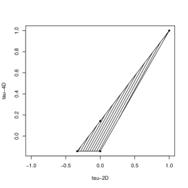
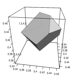
Figure 2: Left panel: set of attainable values of $(\tau_{2},\tau_{4})$ in Example 1. Right panel: Convex polytope of attainable fourth order concordance probabilities in Example 2.

6.3 Data illustration

We now return to the motivating example at the beginning of the paper. Using real data on cryptocurrency returns we illustrate the use of the signature estimation method and we show how missing rank correlation values may be inferred from existing values.

Example 3.

We take the multivariate time series of cryptocurrency prices (in US dollars) for Bitcoin, Ethereum, Litecoin and Ripple. From these data we compute the daily log-returns for the calendar year 2017, giving us 365 4-dimensional data points. The estimated even concordance signature is

$$\bm{\kappa}_{n}=(1,0.639,0.666,0.598,0.681,0.630,0.661,0.364)$$

while the weight vector describing the extremal mixture copula $C$ satisfying $\bm{\kappa}(C)=\bm{\kappa}_{n}$ is

$$\bm{w}=(0.364,0.129,0.069,0.077,0.098,0.075,0.066,0.122),$$

where all figures are given to 3 decimal places. The Kendall rank correlations of the copula $C$ will exactly match the estimated values from the data.

Suppose we are not interested in Ripple but rather in a new cryptocurrency X4coin for which we have no data. We want to estimate the correlations between X4coin and the first three cryptocurrencies. By computing the convex hull of the set of points in (20), and converting the concordance probabilities to Kendall’s tau values, we obtain the polytope shown in the left panel of Figure 1.

Suppose that we now decide that a plausible value for $\tau_{\{1,4\}}$ is 0.598, which is actually the estimated rank correlation between Bitcoin and Ripple implied by the estimated concordance signature above. Then the remaining two values must lie in the convex set shown in the right panel of Figure 1, which is a section of the 3-dimensional set, shown as a cut in the left panel. This is certainly the case for the estimated values of the Etherium-Ripple and Litecoin-Ripple rank correlations which are shown as a point within the set.

7 blackConcordance signatures of elliptical copulas

The concordance signature is identical for the copulas of all continuous elliptical distributions with the same correlation matrix $P$. This follows because the individual probabilities of concordance are identical for all such copulas. This is proved in Genest et al. (2011, Section 2.1) in the context of an analysis of multivariate Kendall’s tau coefficients.

Let $\bm{X}$ have an elliptical distribution centred at the origin with dispersion matrix equal to the correlation matrix $P$ and assume that $\mathbb{P}(\bm{X}=\bm{0})=0$. If $\bm{X}^{*}$ is an independent copy of $\bm{X}$, then the concordance probabilities (1) are given by $\kappa_{I}=2\mathbb{P}\left(\bm{X}_{I}<\bm{X}_{I}^{*}\right)=2\mathbb{P}\left(\bm{X}_{I}-\bm{X}_{I}^{*}<\bm{0}\right)$. The random vector $\bm{X}_{I}-\bm{X}_{I}^{*}$ also has an elliptical distribution centred at the origin. Using the stochastic representation for elliptical distributions (Fang et al., 1990; McNeil et al., 2015) we can write $\bm{X}_{I}-\bm{X}_{I}^{*}\stackrel{{\scriptstyle\text{\tiny d}}}{{=}}R_{1}A\bm{S}$ and $\bm{X}_{I}\stackrel{{\scriptstyle\text{\tiny d}}}{{=}}R_{2}A\bm{S}$ where $\bm{S}$ is a random vector uniformly distributed on the unit sphere, $A$ is a matrix such that $AA^{\top}=P$ and $R_{1}$ and $R_{2}$ are positive scalar random variables, both independent of $\bm{S}$. It follows that

$$\kappa_{I}=2\mathbb{P}\left(\bm{X}_{I}-\bm{X}_{I}^{*}<\bm{0}\right)=2\mathbb{P}\Big{(}(R_{1}A\bm{S})_{I}<\bm{0}\Big{)}=2\mathbb{P}\Big{(}(R_{2}A\bm{S})_{I}<\bm{0}\Big{)}=2\mathbb{P}(\bm{X}_{I}<\bm{0}).$$ (23)

From this calculation, we see that the positive scalar random variable $R_{2}$ plays no role, so that the concordance probabilities $\kappa_{I}$ are the same for any elliptical random vector with the same dispersion matrix $P=AA^{\top}$. Moreover, they are equal to twice the orthant probabilities for a centred elliptical distribution with dispersion matrix $P$. In practice it is easiest to calculate the orthant probabilities of a multivariate normal distribution $\bm{X}\sim\mathcal{N}(\bm{0},P)$ and this is the approach we take in our examples; see B for an illustration involving a $6\times 6$ correlation matrix.

Every linear correlation matrix can be the correlation matrix of a multivariate elliptical (or multivariate normal) distribution. We now show by means of a counterexample that an analogous statement is not true of Kendall rank correlation matrices.

Example 4.

The positive-definite correlation matrix

$$P_{\tau}=\left(\begin{array}[]{rrrr}1&-0.19&-0.29&0.49\\ -0.19&1&-0.34&0.30\\ -0.29&-0.34&1&-0.79\\ 0.49&0.30&-0.79&1\end{array}\right)$$ (24)

is a Kendall rank correlation matrix but is not the Kendall rank correlation matrix of an elliptical distribution. The elements of this matrix are attainable values for the Kendall’s tau coefficients $\tau_{\{i,j\}}$ if the corresponding concordance probabilities $\kappa_{\{i,j\}}=(1+\tau_{\{i,j\}})/2$ are attainable. Using the methods of the previous section we can verify that

$$\bm{\kappa}=(\kappa_{\emptyset},\kappa_{\{1,2\}},\kappa_{\{1,3\}},\kappa_{\{1,4\}},\kappa_{\{2,3\}},\kappa_{\{2,4\}},\kappa_{\{3,4\}})$$

is an attainable partial concordance signature. Solving the linear programming problem (21) gives the weight vector

$$\bm{w}_{1}=(0.04,0.005,0.36,0,0.0625,0.2475,0.2825,0.0025)$$

corresponding to the minimum attainable fourth order concordance probability of 0.04. Solving the linear programming problem (22) gives the weight vector

$$\bm{w}_{2}=(0.0425,0.0025,0.3575,0.0025,0.06,0.25,0.285,0)$$

corresponding to the maximum attainable fourth order concordance probability of 0.0425. In this case $\bm{w}_{1}$ and $\bm{w}_{2}$ are precisely the two vertices of the polytope of attainable weights given by the set (19), which takes the form of a line segment connecting $\bm{w}_{1}$ and $\bm{w}_{2}$. Any weight vector in this set will give the Kendall rank correlation matrix $P_{\tau}$.

Now let us assume that $P_{\tau}$ in (24) corresponds to an elliptical copula. Lindskog et al. (2003) and Fang and Fang (2002) have shown that the Kendall rank correlation matrix of an elliptical copula with correlation matrix $P$ is given by the componentwise transformation $P_{\tau}=2\pi^{-1}\arcsin(P)$. It must be the case that $P=\sin(\pi P_{\tau}/2)$ is the correlation matrix of the elliptical copula. However, by calculating the eigenvalues we find that $P$ is not positive semi-definite, which is a contradiction.

We now turn to the copula of the multivariate Student $t$ distribution $C^{t}_{\nu,P}$ with degree of freedom parameter $\nu$ and correlation matrix parameter $P$. It is unusual to consider this copula for degrees of freedom $\nu<1$, but blackas it turns out, the Student $t$ copula converges to an extremal mixture as $\nu\to 0$. The proof of the following remarkable property relies on some limiting results for the univariate and multivariate $t$ distribution which are collected in C.

Theorem 4.

As $\nu\to 0$ the $d$-dimensional $t$ copula $C^{t}_{\nu,P}$ converges pointwise to the unique extremal mixture copula that shares its concordance signature.

Proof.

Let the function $h_{\nu}(w,\bm{s})$ be defined by

$$h_{\nu}(w,\bm{s})=F_{\nu}\left(G_{d,\nu}^{-1}(w)A\bm{s}\right),\quad w\in(0,1),\quad\bm{s}=(s_{1},\ldots,s_{d}),\;\bm{s}^{\top}\bm{s}=1,$$

where $F_{\nu}$ is the distribution function of a $t$ distribution with $\nu$ degrees of freedom, $G_{d,\nu}$ is the distribution function of the radial component of a $d$-dimensional multivariate $t$ distribution with $\nu$ degrees of freedom and $A$ is a $d\times d$ matrix such that $AA^{\top}=P$; such a matrix can be constructed for any positive semi-definite $P$. Let $\bm{S}=(S_{1},\ldots,S_{d})$ be uniformly distributed on the unit sphere and let $W$ be an independent uniform random variable. Then $\bm{X}=G_{d,\nu}^{-1}(W)A\bm{S}$ has a multivariate $t$ distribution and $\bm{U}=h_{\nu}(W,\bm{S})$ has joint distribution function $C_{\nu.P}^{t}$. We want to show that the joint distribution function of $h_{\nu}(W,\bm{S})$ converges to the joint distribution function of an extremal mixture as $\nu\to 0$.

We first argue that the random vector given by $A\bm{S}$ satisfies $\mathbb{P}\big{(}(A\bm{S})_{j}=0\big{)}=0$. Let $\bm{a}_{j}$ denote the $j$th row of $A$. If $\bm{a}_{j}=\bm{0}$ then the $j$th row and column of $P$ would consist of zeros implying that the $j$th margin of the multivariate $t$ distribution of $\bm{X}$ was degenerate; this case can be discounted because the $t$ copula with such a matrix $P$ is not defined. Suppose therefore that $\mathbb{P}(\bm{a}_{j}^{\top}\bm{S}=0)>0$ for $\bm{a}_{j}\neq\bm{0}$. If $R$ is the radial random variable corresponding to the multivariate normal, then $\mathbb{P}(\bm{a}_{j}^{\top}R\bm{S}=0)=\mathbb{P}(\bm{a}_{j}^{\top}\bm{Z}=0)>0$, where $\bm{Z}$ is a vector of $d$ independent standard normal variables. However $\bm{a}_{j}^{\top}\bm{Z}$ is univariate normal with variance $\bm{a}_{j}^{\top}\bm{a}_{j}>0$ and cannot have an atom of mass at zero.

We can therefore define the set $\mathcal{A}=\{\bm{s}:\bm{s}^{\top}\bm{s}=1,(A\bm{s})_{j}\neq 0,j=1,\ldots,d\}$ such that $\mathbb{P}(\bm{S}\in\mathcal{A})=1$. Given that $\bm{S}=\bm{s}\in\mathcal{A}$, then

$$\{U_{j}\leqslant u_{j}\} =\left\{W\leqslant G_{d,\nu}\left(\frac{F_{\nu}^{-1}(u_{j})}{(A\bm{s})_{j}}\right)\right\}\;\text{if $(A\bm{s})>0$,}$$

$$\{U_{j}\leqslant u_{j}\} =\left\{W\geqslant G_{d,\nu}\left(\frac{F_{\nu}^{-1}(u_{j})}{(A\bm{s})_{j}}\right)\right\}\;\text{if $(A\bm{s})<0$,}$$

and hence the conditional distribution function of $\bm{U}$ given $\bm{S}=\bm{s}$ has the form

$$\mathbb{P}(U_{1}\leqslant u_{1},\ldots,U_{d}\leqslant u_{d}|\bm{S}=\bm{s}) =\mathbb{P}\left(\max_{j\not\in I_{A\bm{s}}}\left\{G_{d,\nu}\left(\frac{F_{\nu}^{-1}(u_{j})}{(A\bm{s})_{j}}\right)\right\}\leqslant W\leqslant\min_{j\in I_{A\bm{s}}}\left\{G_{d,\nu}\left(\frac{F_{\nu}^{-1}(u_{j})}{(A\bm{s})_{j}}\right)\right\}\right)$$

$$=\left(\min_{j\in I_{A\bm{s}}}\left\{G_{d,\nu}\left(\frac{F_{\nu}^{-1}(u_{j})}{(A\bm{s})_{j}}\right)\right\}-\max_{j\not\in I_{A\bm{s}}}\left\{G_{d,\nu}\left(\frac{F_{\nu}^{-1}(u_{j})}{(A\bm{s})_{j}}\right)\right\}\right)^{+},$$

where $I_{A\bm{s}}$ is the set of indices $j$ for which $(A\bm{s})_{j}>0$. Writing, for any $\bm{u}\in(0,1)^{d}$,

$$C_{\nu.P}^{t}(\bm{u})=\mathbb{P}(U_{1}\leqslant u_{1},\ldots,U_{d}\leqslant u_{d})=\int\mathbb{P}(U_{1}\leqslant u_{1},\ldots,U_{d}\leqslant u_{d}|S=\bm{s})dF_{\bm{S}}(\bm{s}),$$

we can use Proposition 8 in C and Lebesgue’s Dominated Convergence Theorem to conclude that $C_{\nu.P}^{t}(\bm{u})$ converges, as $\nu\to 0$, to

$$C(\bm{u})=\int\left(\min_{j\in I_{A\bm{s}}}(2u_{j}-1)^{+}-\max_{j\not\in I_{A\bm{s}}}(1-2u_{j})^{+}\right)^{+}dF_{\bm{S}}(\bm{s}).$$ (25)

We now show that this limit is a mixture of extremal copulas. To this end, consider the random vector $\big{(}\operatorname{sign}(A\bm{S})+\bm{1}\big{)}/2$. This has the same distribution as the multivariate Bernoulli random vector $\bm{Y}$ whose distribution is defined by the probabilities $p_{I}=\mathbb{P}(\bm{Y}_{I}=\bm{1})=\mathbb{P}\big{(}(A\bm{S})_{j}>0,j\in I\big{)}$ for $I\subseteq\mathcal{D}$; the random vectors $\big{(}\operatorname{sign}(A\bm{S})+\bm{1}\big{)}/2$ and $\bm{Y}$ differ only on the null set where components of $A\bm{S}$ are zero. Moreover, the distribution of $\bm{Y}$ is radially symmetric since the spherical symmetry of $\bm{S}$ implies $A\bm{S}\stackrel{{\scriptstyle\text{\tiny d}}}{{=}}-A\bm{S}$ which in turn implies $\bm{Y}\stackrel{{\scriptstyle\text{\tiny d}}}{{=}}\bm{1}-\bm{Y}$. The limiting distribution (25) may be written in the form

$$C(\bm{u})=\sum_{\bm{y}\in\{0,1\}^{d}}\left(\min_{j:y_{j}=1}(2u_{j}-1)^{+}-\max_{j:y_{j}=0}(1-2u_{j})^{+}\right)^{+}\mathbb{P}(\bm{Y}=\bm{y})$$

and using the index set notation defined in Section 3 this may also be written as

$$C(\bm{u}) =\sum_{k=1}^{2^{d-1}}\left(\min_{j\in J_{k}}(2u_{j}-1)^{+}-\max_{j\in J_{k}^{\complement}}(1-2u_{j})^{+}\right)^{+}\mathbb{P}(\bm{Y}=\bm{s}_{k})$$

$$+\sum_{k=1}^{2^{d-1}}\left(\min_{j\in J_{k}^{\complement}}(2u_{j}-1)^{+}-\max_{j\in J_{k}}(1-2u_{j})^{+}\right)^{+}\mathbb{P}(\bm{Y}=\bm{1}-\bm{s}_{k})\;.$$

Setting $\mathbb{P}(\bm{Y}=\bm{s}_{k})=\mathbb{P}(\bm{Y}=\bm{1}-\bm{s}_{k})=0.5w_{k}$ as in Section 3 we obtain $C(\bm{u})=\sum_{k=1}^{2^{d-1}}w_{k}C_{k}(\bm{u})$, where

$$2C_{k}(\bm{u})=\left(\min_{j\in J_{k}}(2u_{j}-1)^{+}-\max_{j\in J_{k}^{\complement}}(1-2u_{j})^{+}\right)^{+}+\left(\min_{j\in J_{k}^{\complement}}(2u_{j}-1)^{+}-\max_{j\in J_{k}}(1-2u_{j})^{+}\right)^{+}$$

and we need to check that $C_{k}$ is in fact the $k$th extremal copula $C^{(k)}$ given by (5). To do so, we have to distinguish the four cases below:

1. Suppose that there is at least one $j\in J_{k}$ and at least one $j\in J_{k}^{\complement}$ such that $u_{j}\leqslant 0.5$. Then $C_{k}(\bm{u})=0=C^{(k)}(\bm{u})$.

2. Suppose that for all $j\in J_{k}$, $u_{j}>0.5$ and there exists at least one $j\in J_{k}^{\complement}$ such that $u_{j}\leqslant 0.5$. Then $2C_{k}(\bm{u})$ equals

   $$\left(\min_{j\in J_{k}}(2u_{j}-1)-\max_{j\in J_{k}^{\complement}}(1-2u_{j})\right)^{+}=2\left(\min_{j\in J_{k}}u_{j}+\min_{j\in J_{k}^{\complement}}u_{j}-1\right)^{+}=2C^{(k)}(\bm{u}).$$

3. The case when for all $j\in J_{k}^{\complement}$, $u_{j}>0.5$ and there exists at least one $j\in J_{k}$ such that $u_{j}\leqslant 0.5$ is analogous to case (ii) and is omitted.

4. Suppose that for all $j\in\mathcal{D}$, $u_{j}>0.5$. Then

   $$2C_{k}(\bm{u})=\min_{j\in J_{k}}(2u_{j}-1)+\min_{j\in J_{k}^{\complement}}(2u_{j}-1)=2\left(\min_{j\in J_{k}}u_{j}+\min_{j\in J_{k}^{\complement}}u_{j}-1\right)=2C^{(k)}(\bm{u}).$$

Finally, we need to verify that the concordance signature of the limiting mixture of extremal copulas is the same as the concordance signature of $C^{t}_{\nu,P}$ for any $\nu>0$. If $\kappa_{I}$ denotes a concordance probability for the $t$ copula, we need to show that $\kappa_{I}=\sum_{k=1}^{2^{d-1}}w_{k}a_{I,k}$, which is the corresponding concordance probability for the limit. Recall that the vector $\bm{X}=G_{d,\nu}^{-1}(W)A\bm{S}$ has a multivariate $t$ distribution. Equation (23) implies that

$$\kappa_{I}=2\mathbb{P}\left(G_{d,\nu}^{-1}(W)(A\bm{S})_{I}<\bm{0}\right)=2\mathbb{P}\Big{(}(A\bm{S})_{I}<\bm{0}\Big{)}=2\mathbb{P}(\bm{Y}_{I}=\bm{0})=2\mathbb{P}(\bm{Y}_{I}=\bm{1})=\sum_{k=1}^{2^{d-1}}w_{k}a_{I,k},$$

where the final step uses the reasoning employed in the proof of Theorem 1. ∎

Figure 3 shows a scatterplot of the copula $C^{t}_{\nu,P}$ when $\nu=0.03$ and $P=(\rho_{ij})$ is the $3\times 3$ matrix with elements $\rho_{12}=0.2$, $\rho_{13}=0.5$ and $\rho_{23}=0.8$. Clearly the points are distributed very close to the four diagonals of the unit cube. The limiting weights attached to extremal copulas associated with each diagonal are given in Table 1.

Remark 5.

The proof holds even when the matrix $P$ is not of full rank. However, because in such cases the copula is distributed on a strict subspace of the unit hypercube $[0,1]^{d}$, the limiting extremal mixture copula has zero mass on certain diagonals of the hypercube. Suppose, for example, that rows $i$ and $j$ of the matrix $A$ satisfying $AA^{\top}=P$ are identical. Then the components $Y_{i}$ and $Y_{j}$ of the vector $\bm{Y}$ defined in the proof are identical, i.e., they are both $0$ or both $1$. For any vector $\bm{s}_{k}$ such that $s_{k,i}\neq s_{k,j}$ it must be the case that $w_{k}=\mathbb{P}(\bm{Y}=\bm{s}_{k})+\mathbb{P}(\bm{Y}=\bm{1}-\bm{s}_{k})=0$ and so the $k$th diagonal would have zero mass.

Figure 3: Scatterplot of data with distribution $C^{t}_{\nu,P}$ when $\nu=0.03$ and $P$ is the $3\times 3$ matrix with elements $\rho_{12}=0.2$, $\rho_{13}=0.5$ and $\rho_{23}=0.8$.

Table 1: Probabilities associated with diagonals of unit cube for copula in Figure 3.

Diagonal	Probability
$(0,0,0)\leftrightarrow(1,1,1)$	51.3%
$(0,0,1)\leftrightarrow(1,1,0)$	5.1%
$(0,1,0)\leftrightarrow(1,0,1)$	15.4%
$(0,1,1)\leftrightarrow(1,0,0)$	28.2%

8 blackConcordance signatures of equiconcordant copulas

As we saw in Example 1, the constraint that certain concordance probabilities are equal further restricts the set of attainable signatures. We close this paper by investigating this phenomenon in greater detail. To this end, let $\Pi(\bm{u})$ represent a permutation of the vector $\bm{u}=(u_{1},\ldots,u_{d})$ and recall that a copula $C$ is said to be exchangeable if $C(\Pi(\bm{u}))=C(\bm{u})$ for all $\bm{u}\in[0,1]^{d}$ and any permutation $\Pi$. A weaker notion of symmetry based on concordance signatures is the following:

Definition 3.

A copula $C$ is said to be equiconcordant if its even concordance signature $\bm{\kappa}(C)=\left\{\kappa_{I}:I\in\mathcal{E}(\mathcal{D})\right\}$ has the property that $\kappa_{I}=\kappa_{\tilde{I}}$ whenever $|I|=|\tilde{I}|$.

Every exchangeable copula $C$ is equiconcordant but not every equiconcordant copula is exchangeable. However, as we will show, the notions are equivalent for the class of extremal mixture copulas.

To develop the necessary arguments we introduce some further notation for extremal copulas building on the notation of Section 3. Let $\eta_{k}=\max(|J_{k}|,|J_{k}^{\complement}|)$ define the comonotonic number of the extremal copula $C^{(k)}$ or, in other words, the size of the larger of the two groups of comonotonic random variables described by $C^{(k)}$. If we order the distinct values of $\eta_{k}$ from largest to smallest we obtain a vector $(h_{1},\ldots,h_{m(d)})=(d,d-1,\ldots,\lceil d/2\rceil)$ with $m(d)=1+\lfloor d/2\rfloor$ elements, where $\lfloor\cdot\rfloor$ and $\lceil\cdot\rceil$ are the floor and ceiling functions respectively.

Each value $h_{i}$ can be associated with a multiplicity, which is the number of extremal copulas with comonotonic number $h_{i}$. Provided $d\neq 2h_{i}$, the multiplicity is the number of ways of choosing the $h_{i}$ members of the larger comonotonic group from a set of $d$ variables and is therefore $\mu_{i}=\tbinom{d}{h_{i}}$. When $d=2h_{i}$ the binomial coefficient double counts the number of extremal copulas with comonotonic number $h_{i}$; for example the extremal copula for which the first $h_{i}$ variables are comonotonic is identical to the extremal copula for which the last $h_{i}$ variables are comonotonic. Thus, in this case, the mutiplicity is given by $\mu_{i}=\tfrac{1}{2}\tbinom{d}{h_{i}}$.

To understand the notation it is helpful to consider a concrete case. When $d=4$ we have $\eta_{1}=4$, $\eta_{2}=\eta_{3}=\eta_{5}=\eta_{8}=3$ and $\eta_{4}=\eta_{6}=\eta_{7}=2$; thus in this case the 8 extremal copulas can be split into $m(4)=3$ groups according to comonotonic number and we find $(h_{1},h_{2},h_{3})=(4,3,2)$ and $(\mu_{1},\mu_{2},\mu_{3})=(1,4,3)$.

We also need to consider the behaviour of extremal copulas under permutations of the arguments. Clearly, the first extremal copula $C^{(1)}$ is exchangeable, but the others are not. For example, under the permutation $\Pi(\bm{u})=(u_{3},u_{4},u_{1},u_{2})$ we find that

$$C^{(2)}(\Pi(\bm{u}))=(\min(u_{3},u_{4},u_{1})+u_{2}-1)^{+}=(\min_{j\in J_{5}}u_{j}+\min_{j\in J_{5}^{\complement}}u_{j}-1)^{+}=C^{(5)}(\bm{u}).$$

and, more generally, $C^{(2)}\to C^{(5)}\to C^{(2)}$, $C^{(3)}\to C^{(8)}\to C^{(3)}$, $C^{(4)}\to C^{(4)}$, $C^{(6)}\to C^{(6)}$ and $C^{(7)}\to C^{(7)}$. It is clear that every extremal copula is mapped either to itself or to another extremal copula with the same comonotonic number. For other permutations the mapping may differ and extremal copulas may form cycles of length greater than two, but they will always be mapped to copulas with the same comonotonic number.

Proposition 7.

Let $C^{*}=\sum_{k=1}^{2^{d-1}}w_{k}C^{(k)}$ be an extremal mixture copula. The following statements are equivalent:

1. $C^{*}$ is exchangeable.

2. $C^{*}$ is equiconcordant.

3. For all $k,l\in\{1,\ldots,2^{d-1}\}$ the weights satisfy $w_{k}=w_{l}$ whenever $\eta_{k}=\eta_{l}$.

Proof.

We show that $1\Rightarrow 2\Rightarrow 3\Rightarrow 1$. The first of these implications is immediate. If $I$ and $\tilde{I}$ are two subsets of $\mathcal{D}$ with the same cardinality then exchangeability implies $C^{*}_{I}=C^{*}_{\tilde{I}}$ and therefore $\kappa_{I}=\kappa(C^{*}_{I})=\kappa(C^{*}_{\tilde{I}})=\kappa_{\tilde{I}}$.

$2\Rightarrow 3$. We use an inductive argument based on comonotonic number $h_{i}$ for $i\in\{1,\ldots,m(d)\}$. Observe first that for $i=1$ the set $I=\mathcal{D}$ is the single subset of $\mathcal{D}$ with cardinality $|I|=d=h_{1}$ and in this case $\kappa_{I}=w_{1}$, the weight on the first extremal copula $C^{(1)}$, which is the only extremal copula with comonotonic number $h_{1}$. Now suppose that $w_{k}=w_{l}$ whenever $\eta_{k}=\eta_{l}=h_{j}$ for all $j\in\{1,\ldots,i\}$ and $i<m(d)$. We want to show that $w_{k}=w_{l}$ whenever $\eta_{k}=\eta_{l}=h_{i+1}$. Consider the subsets $I$ such that $|I|=h_{i+1}$. For each of these subsets we have a formula for the concordance probability of the form $\kappa(C^{*}_{I})=\sum_{k=1}^{2^{d-1}}w_{k}a_{I,k}$ by Proposition 4 and if $a_{I,k}=1$ it must be the case that $\eta_{k}\geqslant h_{i+1}$ by (10). For each distinct subset $I$ there is an equal number of copulas $C^{(k)}$ with $a_{I,k}=1$ and $\eta_{k}=h_{j}$ for each $j\in\{1,\ldots,i\}$ and, by assumption, the weights on copulas with the same comonotonic number are equal. If $h_{i+1}\neq d/2$ there are $\mu_{i+1}$ extremal copulas $C^{(k)}$ with $\eta_{k}=h_{i+1}$ and $\mu_{i+1}$ sets $I$ with $|I|=h_{i+1}$ and for each distinct set $I$ there is a distinct extremal copula $C^{(k)}$ such that $a_{I,k}=1$. If $h_{i+1}=d/2$ there are $\mu_{i+1}$ extremal copulas with $\eta_{k}=h_{i+1}$ and $2\mu_{i+1}$ sets $I$ with $|I|=h_{i+1}$; in this case each distinct set $I$ is weighted on a single extremal copula but for each $C^{(k)}$ there are two sets $I$ with $a_{I,k}=1$. In either case, the equality of the concordance probabilities for the sets $I$ implies that the weights $w_{k}$ are identical for all copulas with $\eta_{k}=h_{i+1}$.

$3\Rightarrow 1$. For a permutation $\Pi$ let the function $l_{\Pi}(k)$ give the identity of the extremal copula to which $C^{(k)}$ is mapped under $\Pi$ and recall that this copula has the same comonotonic number as $C^{(k)}$. Then, for all $\bm{u}\in[0,1]^{d}$,

$$C^{*}(\Pi(\bm{u}))=\sum_{k=1}^{2^{d-1}}w_{k}C^{(k)}(\Pi(\bm{u}))=\sum_{k=1}^{2^{d-1}}w_{k}C^{(l_{\Pi}(k))}(\bm{u})=\sum_{k=1}^{2^{d-1}}w_{l_{\Pi}(k)}C^{(l_{\Pi}(k))}(\bm{u})$$

where the final step follows because $w_{k}=w_{l}$ whenever $\eta_{k}=\eta_{l}$. To complete the proof we need to show that the function $l_{\Pi}$ is simply a permutation of the indices $k=1,\ldots,2^{d-1}$ implying that $C^{*}(\Pi(\bm{u}))=C^{*}(\bm{u})$. To see this assume that $l_{\pi}(k_{1})=l_{\Pi}(k_{2})$ for $k_{1}\neq k_{2}$ so that, for any $\bm{u}\in[0,1]^{d}$,

$$C^{(k_{1})}(\Pi(\bm{u}))=C^{l(k_{1})}(\bm{u})=C^{l(k_{2})}(\bm{u})=C^{(k_{2})}(\Pi(\bm{u})).$$

If $\Pi^{-1}$ denotes the inverse permutation satisfying $\Pi(\Pi^{-1}(\bm{u}))=\bm{u}$, then this would imply that

$$C^{(k_{1})}(\bm{u})=C^{l(k_{1})}(\Pi^{-1}(\bm{u}))=C^{l(k_{2})}(\Pi^{-1}(\bm{u}))=C^{(k_{2})}(\bm{u})$$

contradicting the assumption that $k_{1}\neq k_{2}$. ∎

This result allows us to conclude that for any equiconcordant copula $C$, the extremal mixture copula $C^{*}$ sharing its signature with $C$ is exchangeable. Moreover, we can infer that the set of attainable even equiconcordance signatures takes the form

$$\left\{\sum_{k=1}^{2^{d-1}}w_{k}\bm{a}_{k}:w_{k}\geqslant 0,\sum_{k=1}^{2^{d-1}}w_{k}=1,w_{k}=w_{l}\;\text{if}\;\eta_{k}=\eta_{l},\forall k,l\in\{1,\ldots,2^{d-1}\}\right\}$$

and we can write this in a simplifed way as

$$\left\{\sum_{i=1}^{m(d)}v_{i}\bm{b}_{i}:v_{i}\geqslant 0,\sum_{i=1}^{m(d)}v_{i}=1\right\},\quad\bm{b}_{i}=\frac{1}{\mu_{i}}\sum_{k=1}^{2^{d-1}}\bm{a}_{k}\mathbbm{1}_{\{\eta_{k}=h_{i}\}}$$

where we note that the vectors $\bm{b}_{i}$ are obtained by averaging the vectors $\bm{a}_{k}$ corresponding to extremal copulas with the same comonotonic number and are linearly independent (because the vectors $\bm{a}_{k}$ are linearly independent). The weights $v_{i}$ now express the total weight assigned to all copulas with the same comonotonic number. The set of attainable equiconcordance signatures is clearly also a convex polytope with vertices given by the vectors $\bm{b}_{1},\ldots,\bm{b}_{m(d)}$.

The $2^{d-1}\times m(d)$ matrix with columns $\bm{b}_{i}$ has identical rows corresponding to sets $I$ and $\tilde{I}$ with identical cardinality. Duplicate rows can simply be dropped to retain exactly $m(d)$ rows corresponding to each distinct even cardinality in the set $E=\{0,2,\ldots,2\lfloor d/2\rfloor\}$. This results in an invertible square matrix $B_{d}$. Let us write the elements of the even concordance signature corresponding to each distinct cardinality as $\bm{k}=(\kappa_{i}:i\in E)$ and refer to $\bm{k}$ as the skeletal signature of an equiconcordant copula. We can then consider the linear equation system $\bm{k}=B_{d}\bm{v}$ to solve attainability and compatibility problems for skeletal signatures.

For example, the equation system for $d=7$ is

$$\overbrace{\left(\begin{array}[]{c}1\\ \kappa_{2}\\ \kappa_{4}\\ \kappa_{6}\end{array}\right)}^{\bm{k}}=\overbrace{\left(\begin{array}[]{cccc}1&1&1&1\\[3.0pt] 1&\frac{5}{7}&\frac{11}{21}&\frac{15}{35}\\[3.0pt] 1&\frac{3}{7}&\frac{3}{21}&\frac{1}{35}\\[3.0pt] 1&\frac{1}{7}&0&0\end{array}\right)}^{B_{7}}\overbrace{\left(\begin{array}[]{c}v_{1}\\ v_{2}\\ v_{3}\\ v_{4}\end{array}\right)}^{\bm{v}}$$

and the columns of $B_{7}$ form the 4 vertices of the convex polytope of attainable vectors for the skeletal signature; upon removal of the 1’s in the first component these describe an irregular tetrahedron inside the unit cube $[0,1]^{3}$ as shown in Figure 4.

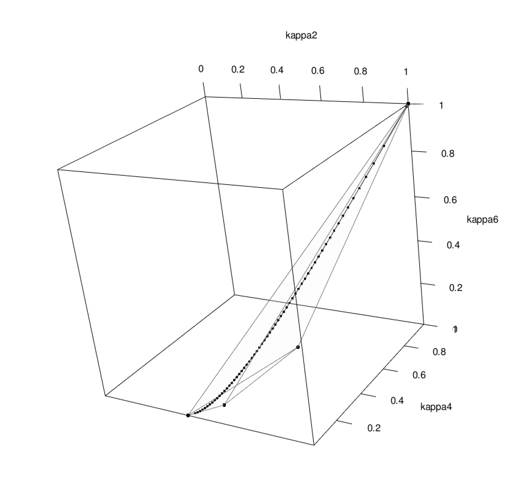
Figure 4: The tetrahedron is the set of attainable skeletal concordance signatures of equiconcordant copulas when $d=7$. The curve and associated points within the tetrahedron show the attainable skeletal signatures of exchangeable elliptical copulas.

In higher dimensions it quickly becomes computationally infeasible to calculate the matrix $B_{d}$ by collapsing the $2^{d-1}\times 2^{d-1}$ matrix $A_{d}$. We end by giving a general formula for the elements of the matrix $B_{d}$ using combinatorial arguments.

Theorem 5.

The elements of the matrix $B_{d}$ satisfy $B_{d}(1,j)=1$ for $j\in\{1,\ldots,m(d)\}$ and

$$B_{d}(i,j)=\frac{\left(\begin{array}[]{c}d-l_{i}\\ h_{j}-l_{i}\end{array}\right)+\left(\begin{array}[]{c}d-l_{i}\\ d-h_{j}-l_{i}\end{array}\right)}{\left(\begin{array}[]{c}d\\ h_{j}\end{array}\right)},\quad i\in\{2,\ldots,m(d)\},\;j\in\{1,\ldots,m(d)\},$$

where $l_{i}=2(i-1)$, $h_{j}$ is the $j$th distinct value of the comonotonic number in reverse order from largest to smallest and, by convention, $\tbinom{n}{p}=0$ if $p<0$.

Proof.

Obviously the first row of $B_{d}$ consists of ones corresponding to the sum constraint on the weights so let $i>1$. To begin with, we exclude the case where $d$ is even and $h_{j}=d/2$. In all other cases the denominator of the fraction above is the multiplicity $\mu_{j}$ of the comonotonic number $h_{j}$. Let $I\subseteq\mathcal{D}$ be any subset with cardinality $|I|=l_{i}$. The numerator is the number of columns of the matrix $A_{d}$ that correspond to extremal copulas with comonotonic number $h_{j}$ and which have a one in the row corresponding to $I$.

Without loss of generality let us consider the set $I$ consisting of the first $l_{i}$ elements of $\mathcal{D}$. In this case we need to simply count the number of extremal copulas $C^{(k)}$ with comonotonic number $h_{j}$ for which the vectors $\bm{s}_{k}$ that we use to code the extremal copulas have zeros in the first $l_{i}$ entries. Now there are two possibilities: either the comonotonic number of the extremal copula $C^{(k)}$ equals the numbers of zeros in the vector $\bm{s}_{k}$ or the number of ones. In the first case, if there are zeros in the first $l_{i}$ positions of $\bm{s}_{k}$ there are $\tbinom{d-l_{i}}{h_{j}-l_{i}}$ ways of assigning the remaining zeros to the other positions. In the second case case there are $\tbinom{d-l_{i}}{d-h_{j}-l_{i}}$ ways of assigning the remaining zeros to the other positions. If either $h_{j}-l_{i}<0$ or $d-h_{j}-l_{i}<0$ then the corresponding binomial coefficients are simply zero.

In the case where $d$ is even and $h_{j}=d/2$ the denominator is twice the multiplicity $\mu_{j}$ of the comonotonic number $h_{j}$. In this case there are exactly the same number of zeros and ones in the $\mu_{j}$ vectors $\bm{s}_{k}$ coding extremal copulas with comonotonic number $h_{j}$ and so there are $\tbinom{d-l_{i}}{h_{j}-l_{i}}$ ways of assigning the remaining zeros to the other positions. However, since $\tbinom{d-l_{i}}{h_{j}-l_{i}}=\tbinom{d-l_{i}}{d-h_{j}-l_{i}}$ when $h_{j}=d/2$, we can use the same general formula. ∎

Software

The methods and examples in this paper are documented in the R package KendallSignature at https://github.com/ajmcneil/KendallSignature.

Appendix A Additional material on extremal mixture copulas

Proof of Proposition 1. Let $\boldsymbol{U}$ be of the form (6) where $U$ and $\boldsymbol{B}$ are independent. For any $\boldsymbol{u}\in[0,1]$,

$$\mathbb{P}(\boldsymbol{U}\leqslant\boldsymbol{u}) =\sum_{\boldsymbol{b}\in\{0,1\}^{d}}\mathbb{P}(\max_{j:b_{j}=0}(1-v_{j})\leqslant U\leqslant\min_{j:b_{j}=1}v_{j}|\boldsymbol{B}=\boldsymbol{b})\mathbb{P}(\boldsymbol{B}=\boldsymbol{b})$$

$$=\sum_{\boldsymbol{b}\in\{0,1\}^{d}}\left(\min_{j:b_{j}=1}v_{j}+\min_{j:b_{j}=0}v_{j}-1\right)^{+}\mathbb{P}(\boldsymbol{B}=\boldsymbol{b})$$

$$=\sum_{k=1}^{2^{d-1}}\left(\min_{j\in J_{k}}v_{j}+\min_{j\in J_{k}^{\complement}}v_{j}-1\right)^{+}\Big{(}\mathbb{P}(\boldsymbol{B}=\boldsymbol{s}_{k})+\mathbb{P}(\boldsymbol{B}=\bm{1}-\boldsymbol{s}_{k})\Big{)}.$$

where in the final step we have used the fact that the set of possible outcomes of the Bernoulli vector $\bm{B}$ can be written as the disjoint union

$$\{0,1\}^{d}=\bigcup_{k=1}^{2^{d-1}}\{\bm{s}_{k},\bm{1}-\bm{s}_{k}\}.$$ (26)

From (5), one can see that the distribution function of $\boldsymbol{U}$ is indeed an extremal mixture with weights as given in (7).

Conversely, given an extremal mixture copula of the form $C^{*}=\sum_{k=1}^{2^{d-1}}w_{k}C^{(k)}$, it suffices to consider any Bernoulli vector $\bm{B}$ independent of $U$ with the property that $w_{k}=\mathbb{P}(\boldsymbol{B}=\boldsymbol{s}_{k})+\mathbb{P}(\boldsymbol{B}=\bm{1}-\boldsymbol{s}_{k})$; this is possible because the events $\{\boldsymbol{B}=\boldsymbol{s}_{k}\}$ and $\{\boldsymbol{B}=\bm{1}-\boldsymbol{s}_{k}\}$ are disjoint and their union forms a partition of $\{0,1\}^{d}$ by (26). We can then retrace the steps of the argument in reverse to establish the representation (6). ∎

Proof of Proposition 2. For part (i), note that all probabilities of the form $p_{I}=\mathbb{P}(\bm{Y}_{I}=\bm{1})$ for sets $I$ with odd cardinality are fully determined by the equivalent probabilities for lower-dimensional sets of even cardinality. This follows from the fact that

$$p_{I}=\mathbb{E}\left(\prod_{i\in I}Y_{i}\right)=\mathbb{E}\left(\prod_{i\in I}(1-Y_{i})\right)=1+\sum_{A\subseteq I,|A|\geqslant 1}(-1)^{|A|}\mathbb{E}\left(\prod_{i\in A}Y_{i}\right).$$

When $I$ is odd, we then have

$$2p_{I}=1+\sum_{A\subset I,1\leqslant|A|<|I|}(-1)^{|A|}p_{A}=1-\tfrac{1}{2}|I|+\sum_{A\subset I,2\leqslant|A|<|I|}(-1)^{|A|}p_{A},$$ (27)

where the last equality follows from the fact that $p_{A}=0.5$ whenever $|A|=1$. For example,

$$p_{\{1,2,3\}} =\mathbb{E}\Big{(}(1-Y_{1})(1-Y_{2})(1-Y_{3})\Big{)}=\frac{1}{2}\left(p_{\{1,2\}}+p_{\{1,3\}}+p_{\{2,3\}}\right)-\frac{1}{4}\;.$$

The conclusion follows since the vector of joint event probabilities $(p_{I}:I\in\mathcal{P}(\mathcal{D})\setminus\emptyset)$ uniquely specifies the distribution of a Bernoulli random vector.

For part (ii) observe that the vector $\bm{p}_{\bm{Y}}$ has length equal to

$$\sum_{j=1}^{\lfloor d/2\rfloor}\left(\begin{array}[]{c}d\\ 2j\end{array}\right)=2^{d-1}-1.$$

Radially symmetric multivariate Bernoulli distributions in dimension $d$ have $2^{d-1}-1$ free parameters, with one being deducted for the sum constraint $2\sum_{k=1}^{2^{d-1}}\mathbb{P}(\bm{Y}=\bm{s}_{k})=1$. Thus the vector $\bm{p}_{\bm{Y}}$ is the minimal vector of its kind that is required to fully specify the distribution of $\bm{Y}$ blackfor all radially symmetric Bernoulli random vectors $\bm{Y}$. ∎

Example 5.

Let the joint distribution of $(U,Y_{1},Y_{2},Y_{3})$ be specified by

$$\mathbb{P}(U\leqslant u,Y_{1}=y_{1},Y_{2}=y_{2},Y_{3}=y_{3})=\frac{1}{8}\left(u+(-1)^{(y_{1}+y_{2}+y_{3})}\frac{\theta u(1-u)}{4}\right)$$

for $u\in[0,1]$ and $y_{i}\in\{0,1\}$, $i\in\{1,2,3\}$. Note that this is an increasing function in $u$ for any fixed $(y_{1},y_{2},y_{3})$ and defines a valid distribution. It may be easily verified, by summing over the outcomes for the $Y_{i}$ variables, that the marginal distribution of $U$ is standard uniform, while letting $u\to 1$ shows that the random vector $\bm{Y}=(Y_{1},Y_{2},Y_{3})$ consists of iid Bernoulli variables with success probability $0.5$ (and is radially symmetric). It may also be verified that the marginal distributions $P(U\leqslant u,Y_{i}=y_{i})=0.5u$ so that the pairs $(U,Y_{i})$ are independent for all $i$, while the marginal distributions $P(U\leqslant u,Y_{i}=y_{i},Y_{j}=y_{j})=0.25u$ so that $(U,Y_{i},Y_{j})$ are mutually independent for all $i\neq j$.

Now consider the vector $\bm{U}=U\bm{Y}+(1-U)(\bm{1}-\bm{Y})$. Since the pairs $(U,Y_{i})$ are independent it is easy to see that the components $U_{i}=UY_{i}+(1-U)(1-Y_{i})$ are uniform, implying that the distribution of $\bm{U}$ is a copula. Since the triples $(U,Y_{i},Y_{j})$ are mutually independent, the bivariate margins of $\bm{U}$ are extremal mixtures by Proposition 1. To calculate the copula $C$ of $\bm{U}$ we observe that, for $\bm{u}=(u_{1},u_{2},u_{3})$,

$$C(u_{1},u_{2},u_{3}) =\sum_{i=1}^{4}\Big{(}\mathbb{P}(\bm{U}\leqslant\bm{u},\bm{Y}=\bm{s}_{k})+\mathbb{P}(\bm{U}\leqslant\bm{u},\bm{Y}=\bm{1}-\bm{s}_{k})\Big{)}=2\sum_{i=1}^{4}\mathbb{P}(\bm{U}\leqslant\bm{u},\bm{Y}=\bm{s}_{k}).$$

The final equality follows because our model has the property that $(U,Y_{1},Y_{2},Y_{3})\stackrel{{\scriptstyle\text{\tiny d}}}{{=}}(1-U,1-Y_{1},1-Y_{2},1-Y_{3})$. This implies that $(\bm{U},\bm{Y})=(U\bm{Y}+(1-U)(\bm{1}-\bm{Y}),\bm{Y})\stackrel{{\scriptstyle\text{\tiny d}}}{{=}}(\bm{U},\bm{1}-\bm{Y})$. The copula $C$ has 4 distinct terms, each associated with a diagonal of the unit cube:

$$4C(u_{1},u_{2},u_{3})=\min(u_{1},u_{2},u_{3})+\frac{\theta}{4}\min(u_{1},u_{2},u_{3})\max(1-u_{1},1-u_{2},1-u_{3})$$

$$+\mathbbm{1}_{\{\min(u_{1},u_{2})+u_{3}-1\geqslant 0\}}\Big{(}\min(u_{1},u_{2})-\frac{\theta}{4}\min(u_{1},u_{2})\max(1-u_{1},1-u_{2})-1+u_{3}+\frac{\theta}{4}u_{3}(1-u_{3})\Big{)}$$

$$+\mathbbm{1}_{\{\min(u_{1},u_{3})+u_{2}-1\geqslant 0\}}\Big{(}\min(u_{1},u_{3})-\frac{\theta}{4}\min(u_{1},u_{3})\max(1-u_{1},1-u_{3})-1+u_{2}+\frac{\theta}{4}u_{2}(1-u_{2})\Big{)}$$

$$+\mathbbm{1}_{\{\min(u_{2},u_{3})+u_{1}-1\geqslant 0\}}\Big{(}\min(u_{2},u_{3})-\frac{\theta}{4}\min(u_{2},u_{3})\max(1-u_{2},1-u_{3})-1+u_{1}+\frac{\theta}{4}u_{1}(1-u_{1})\Big{)}.$$

However, unless $\theta=0$, $C$ is not of the form (5) and is not an extremal mixture copula.

Proof of Proposition 3. If $\bm{U}$ follows an extremal mixture copula then, by Proposition 1, it has the stochastic representation $\bm{U}\stackrel{{\scriptstyle\text{\tiny d}}}{{=}}U\bm{B}+(1-U)(\bm{1}-\bm{B})$ for some Bernoulli random vector $\bm{B}$ and it is clear that all the bivariate margins have the same structure. From the independence of $U$ and $\bm{B}$ we obtain

$$\mathbb{P}\left(U_{1}\leqslant u\mid\mathbbm{1}_{\{U_{j}=U_{1}\}},j\neq 1\right) =\mathbb{P}\left(U\leqslant u\mid\mathbbm{1}_{\{B_{2}=B_{1}\}},\ldots,\mathbbm{1}_{\{B_{d}=B_{1}\}}\right)=\mathbb{P}(U\leqslant u)=u.$$

Conversely, let us suppose that all the bivariate margins of $\bm{U}$ are mixtures of extremal copulas. This implies that almost surely, $\bm{U}$ takes values in the set

$$\bigcap_{i\neq j}\{\bm{u}\in[0,1]^{d}:u_{j}=u_{i}\>\text{or}\>u_{j}=1-u_{i}\},$$

which simplifies to the union $\mathcal{E}$ of the $2^{d-1}$ main diagonals of the unit hypercube, viz.

$$\mathcal{E}=\bigcup_{k=1}^{2^{d-1}}\{\bm{u}\in[0,1]^{d}:u_{j}=u_{1}^{(1-s_{k,j})}(1-u_{1})^{s_{k,j}},j\neq 1\}.$$

Let $E_{k}=\{U_{j}=U_{1}^{(1-s_{k,j})}(1-U_{1})^{s_{k,j}},j\neq 1\}$ represent the event that $\bm{U}$ lies on the $k$th diagonal and set $w_{k}=\mathbb{P}(E_{k})$. By the law of total probability, we get

$$C(\bm{u})=\sum_{k=1}^{2^{d-1}}w_{k}\mathbb{P}(U_{1}\leqslant u_{1},\ldots,U_{d}\leqslant u_{d}\mid E_{k})=\sum_{k=1}^{2^{d-1}}w_{k}\mathbb{P}(U_{1}\in[\max_{j\in J_{k}^{\complement}}(1-u_{j}),\min_{j\in J_{k}}u_{j}]\mid E_{k}).$$

On the diagonals of the hypercube, $\{\bm{U}\in\mathcal{E}\}\cap\{\mathbbm{1}_{\{U_{j}=U_{1}\}}=1-s_{k,j},j\neq 1\}=E_{k}$, so that $w_{k}=\mathbb{P}\{\mathbbm{1}_{\{U_{j}=U_{1}\}}=1-s_{k,j},j\neq 1\}$ and conditioning on the event $E_{k}$ is identical to conditioning on the event $\{\mathbbm{1}_{\{U_{j}=U_{1}\}}=1-s_{k,j},j\neq 1\}$. We thus obtain that

$$C(\bm{u})=\sum_{k=1}^{2^{d-1}}w_{k}\mathbb{P}(U_{1}\in[\max_{j\in J_{k}^{\complement}}u_{j},\min_{j\in J_{k}}u_{j}]\mid\mathbbm{1}_{\{U_{j}=U_{1}\}}=1-s_{k,j},j\neq 1)=\sum_{k=1}^{2^{d-1}}w_{k}C^{(k)}(\bm{u})$$

where the last equality follows from (9) and (5). This shows that $C$ is indeed a mixture of extremal copulas as claimed. ∎

Appendix B Additional material on elliptical distributions

The concordance probabilities for a continuous elliptical distribution the $6\times 6$ correlation matrix

$$P=\frac{1}{16}\left(\begin{array}[]{rrrrrr}16&1&2&3&4&5\\ 1&16&6&7&8&9\\ 2&6&16&10&11&12\\ 3&7&10&16&13&14\\ 4&8&11&13&16&15\\ 5&9&12&14&15&16\end{array}\right)$$ (28)

are given in Table 2, along with the weights of the unique mixture of extremal copulas sharing the same concordance signature.

Table 2: Results for the correlation matrix $P$ in (28).

$k$	$S_{k}$	$w_{k}$	$I$	$\kappa_{I}$
1	$\{0,0,0,0,0,0\}$	0.2627	$\emptyset$	1.0000
2	$\{0,0,0,0,0,1\}$	0.0009	$\{1,2\}$	0.5199
3	$\{0,0,0,0,1,0\}$	0.0131	$\{1,3\}$	0.5399
4	$\{0,0,0,0,1,1\}$	0.0037	$\{1,4\}$	0.5600
5	$\{0,0,0,1,0,0\}$	0.0304	$\{1,5\}$	0.5804
6	$\{0,0,0,1,0,1\}$	0.0037	$\{1,6\}$	0.6012
7	$\{0,0,0,1,1,0\}$	0.0088	$\{2,3\}$	0.6224
8	$\{0,0,0,1,1,1\}$	0.0179	$\{2,4\}$	0.6441
9	$\{0,0,1,0,0,0\}$	0.0579	$\{2,5\}$	0.6667
10	$\{0,0,1,0,0,1\}$	0.0029	$\{2,6\}$	0.6902
11	$\{0,0,1,0,1,0\}$	0.0100	$\{3,4\}$	0.7149
12	$\{0,0,1,0,1,1\}$	0.0108	$\{3,5\}$	0.7413
13	$\{0,0,1,1,0,0\}$	0.0165	$\{3,6\}$	0.7699
14	$\{0,0,1,1,0,1\}$	0.0085	$\{4,5\}$	0.8019
15	$\{0,0,1,1,1,0\}$	0.0063	$\{4,6\}$	0.8391
16	$\{0,0,1,1,1,1\}$	0.0659	$\{5,6\}$	0.8869
17	$\{0,1,0,0,0,0\}$	0.1037	$\{1,2,3,4\}$	0.2804
18	$\{0,1,0,0,0,1\}$	0.0029	$\{1,2,3,5\}$	0.2977
19	$\{0,1,0,0,1,0\}$	0.0114	$\{1,2,3,6\}$	0.3150
20	$\{0,1,0,0,1,1\}$	0.0091	$\{1,2,4,5\}$	0.3244
21	$\{0,1,0,1,0,0\}$	0.0193	$\{1,2,4,6\}$	0.3437
22	$\{0,1,0,1,0,1\}$	0.0073	$\{1,2,5,6\}$	0.3675
23	$\{0,1,0,1,1,0\}$	0.0062	$\{1,3,4,5\}$	0.3702
24	$\{0,1,0,1,1,1\}$	0.0390	$\{1,3,4,6\}$	0.3909
25	$\{0,1,1,0,0,0\}$	0.0338	$\{1,3,5,6\}$	0.4161
26	$\{0,1,1,0,0,1\}$	0.0064	$\{1,4,5,6\}$	0.4581
27	$\{0,1,1,0,1,0\}$	0.0076	$\{2,3,4,5\}$	0.4503
28	$\{0,1,1,0,1,1\}$	0.0232	$\{2,3,4,6\}$	0.4725
29	$\{0,1,1,1,0,0\}$	0.0100	$\{2,3,5,6\}$	0.4993
30	$\{0,1,1,1,0,1\}$	0.0136	$\{2,4,5,6\}$	0.5427
31	$\{0,1,1,1,1,0\}$	0.0036	$\{3,4,5,6\}$	0.6153
32	$\{0,1,1,1,1,1\}$	0.1831	$\{1,2,3,4,5,6\}$	0.2627

Appendix C Some limiting properties of the univariate and multivariate Student distribution as $\nu\to 0$

C.1 Univariate Student $t$ distribution

Let $F_{\nu}$, $F_{\nu}^{-1}$ and $f_{\nu}$ denote the df, inverse df and density of a univariate $t$ distribution with $\nu$ degrees of freedom. The df satisfies

$$F_{\nu}(x)-0.5=\frac{x\Gamma(\frac{\nu+1}{2})}{\sqrt{\pi\nu}\Gamma(\frac{\nu}{2})}{}_{2}F_{1}\left(\frac{1}{2},\frac{\nu+1}{2};\frac{3}{2};-\frac{x^{2}}{\nu}\right),\quad x\in\mathbb{R},\;\nu>0,$$ (29)

where ${}_{2}F_{1}$ denotes the hypergeometric function and $\Gamma$ the gamma function. We will show that, for fixed $u\neq 0.5$, the quantile function $F_{\nu}^{-1}(u)$ is unbounded as a function of $\nu$ as $\nu\to 0$. To that end we first prove the following lemma.

Lemma 2.

$\lim_{\nu\to 0}F_{\nu}(x)=0.5$ for all $x\in\mathbb{R}$.

Proof.

The lemma is trivially true for $x=0$ so we consider $x\neq 0$. Making the substitution $y=x/\sqrt{\nu}$ in (29) gives

$$\frac{2F_{\nu}(\sqrt{\nu}y)-1}{\nu}=\frac{2y\Gamma(\frac{\nu+1}{2})}{\sqrt{\pi}\nu\Gamma(\frac{\nu}{2})}{}_{2}F_{1}\left(\frac{1}{2},\frac{\nu+1}{2};\frac{3}{2};-y^{2}\right)$$

and we can use the limits (Abramowitz and Stegun, 1965)

$$\lim_{\nu\to 0}y\;{}_{2}F_{1}\left(\frac{1}{2},\frac{\nu+1}{2};\frac{3}{2};-y^{2}\right)=y\;{}_{2}F_{1}\left(\frac{1}{2},\frac{1}{2};\frac{3}{2};-y^{2}\right)=\ln\left(y+\sqrt{1+y^{2}}\right)$$

$$\lim_{\nu\to 0}\frac{2\Gamma(\frac{\nu+1}{2})}{\sqrt{\pi}\nu\Gamma(\frac{\nu}{2})}=\lim_{\nu\to 0}\frac{\Gamma(\frac{\nu+1}{2})}{\sqrt{\pi}}\frac{1}{\frac{\nu}{2}\Gamma(\frac{\nu}{2})}=\lim_{\nu\to 0}\frac{\Gamma(\frac{\nu+1}{2})}{\sqrt{\pi}}\frac{1}{\Gamma(\frac{\nu+2}{2})}=1$$

to conclude that

$$\lim_{\nu\to 0}\frac{2F_{\nu}(\sqrt{\nu}y)-1}{\nu}=\ln\left(y+\sqrt{1+y^{2}}\right)=\operatorname{sign}(y)\ln\left(|y|+\sqrt{1+y^{2}}\right).$$

Reversing the earlier substitution and setting $x=\sqrt{\nu}y$ now gives

$$\lim_{\nu\to 0}\frac{2F_{\nu}(x)-1}{\nu\operatorname{sign}(x)\left(\ln\big{(}|x|+\sqrt{\nu+x^{2}}\big{)}-0.5\ln\nu\right)}=1.$$

The result follows from the fact that the denominator tends to 0 as $\nu\to 0$. ∎

Lemma 3.

$$\lim_{\nu\to 0}F_{\nu}^{-1}(u)=\begin{cases}-\infty&\text{if $u<0.5$,}\\ 0&\text{if $u=0.5$,}\\ \infty&\text{if $u>0.5$.}\end{cases}$$

Proof.

The case $u=0$ is obvious, since $F_{\nu}^{-1}(0.5)=0$ for all $\nu>0$. To show that $\lim_{\nu\to 0}F_{\nu}^{-1}(u)=-\infty$ for $u<0.5$, we need to show that, for all $k<0$, there exists $\delta$ such that $\nu<\delta\Rightarrow F_{\nu}^{-1}(u)\leqslant k$. Suppose we fix an arbitrary $k<0$. Since $F_{\nu}(k)\to 0.5$ as $\nu\to 0$, there exists $\delta>0$ such that $\nu<\delta$ implies that $F_{\nu}(k)>u$, since $u<0.5$. But then, for any $\nu<\delta$, it follows that $k\in\{x:F_{\nu}(x)\geqslant u\}$ and hence $F_{\nu}^{-1}(u)=\inf\{x:F_{\nu}(x)\geqslant u\}\leqslant k$.

Analogously, to show that $\lim_{\nu\to 0}F_{\nu}^{-1}(u)=\infty$ for $u>0.5$, we need to show that, for all $k>0$, there exists $\delta$ such that $\nu<\delta\Rightarrow F_{\nu}^{-1}(u)\geqslant k$. Suppose we fix an arbitrary $k>0$. Since $F_{\nu}(k)\to 0.5$ as $\nu\to 0$, there exists $\delta>0$ such that $\nu<\delta$ implies that $F_{\nu}(k)<u$, since $u>0.5$. But then, for any $\nu<\delta$, it follows that $k\notin\{x:F_{\nu}(x)\geqslant u\}$. Since $F_{\nu}(x)$ is a non-decreasing function of $x$, any $y<k$ also satisfies $y\notin\{x:F_{\nu}(x)\geqslant u\}$. Hence $F_{\nu}^{-1}(u)=\inf\{x:F_{\nu}(x)\geqslant u\}\geqslant k$.

∎

C.2 Multivariate Student $t$ distribution

If the random vector $\bm{X}$ has a $d$-dimensional multivariate $t$ distribution with $\nu$ degrees of freedom, then it has the stochastic representation $\bm{X}\stackrel{{\scriptstyle\text{\tiny d}}}{{=}}\bm{\mu}+RA\bm{S}$ where $\bm{S}$ is a uniform random vector on the $d$-dimensional unit sphere, $R$ is an independent, positive, scalar random variable such that $R^{2}/d\sim F(d,\nu)$ (a Fisher–Snedecor $F$ distribution), $\bm{\mu}$ is a location vector and $A$ is a matrix; see Section 6.3 in McNeil et al. (2015). Let $G_{d,\nu}$ denote the df of the radial random variable $R$ and $g_{d,\nu}$ the corresponding density; the latter is given by

$$g_{d,\nu}(r)=\frac{2}{r}\left(1+\frac{\nu}{r^{2}}\right)^{-\frac{d}{2}}\left(1+\frac{r^{2}}{\nu}\right)^{-\frac{\nu}{2}}\frac{\Gamma\left(\frac{\nu+d}{2}\right)}{\Gamma\left(\frac{d}{2}\right)\Gamma\left(\frac{\nu}{2}\right)}.$$ (30)

The following limiting result is key to our analysis of the limiting behaviour of the $t$ copula as $\nu\to 0$. Note that the limiting function on the right-hand side is either the df of a random variable that is uniformly distributed on $[0.5,1]$ or the survival function of a random variable that is uniformly distributed on $[0,0.5]$, depending on the sign of $\lambda$.

Proposition 8.

For a constant $\lambda\neq 0$ and any $u\in[0,1]$,

$$\lim_{\nu\to 0}G_{d,\nu}\left(\frac{F_{\nu}^{-1}(u)}{\lambda}\right)=\begin{cases}(2u-1)^{+}&\text{if $\lambda>0$,}\\ (1-2u)^{+}&\text{if $\lambda<0$.}\end{cases}$$ (31)

Proof.

When $\lambda>0$, $F_{d,\nu}(u)=G_{d,\nu}\left(\lambda^{-1}F_{\nu}^{-1}(u)\right)$ is a distribution function supported on $[0.5,1]$. Similarly, when $\lambda<0$, $F_{d,\nu}(u)=1-G_{d,\nu}\left(\lambda^{-1}F_{\nu}^{-1}(u)\right)$ is a distribution function supported on $[0,0.5]$. The density of $F_{d,\nu}$ is given by

$$f_{d,\nu}(u) =g_{d,\nu}\left(\frac{|F_{\nu}^{-1}(u)|}{|\lambda|}\right)\frac{1}{|\lambda|}\frac{1}{f_{\nu}\big{(}F_{\nu}^{-1}(u)\big{)}}$$

where $u\in[0.5,1)$ when $\lambda>0$ and $u\in(0,0.5]$ when $\lambda<0$.

Note that, when $u=0.5$, $F_{\nu}^{-1}(u)=0$ for all $\nu$ and (31) clearly holds; we thus restrict our analysis of the density to the case where $u\neq 0.5$. Using the notation $x_{\nu,u}=F_{\nu}^{-1}(u)$ and the expression (30) we have that

$$f_{d,\nu}(u) =g_{d,\nu}\left(\frac{|x_{\nu,u}|}{|\lambda|}\right)\frac{1}{|\lambda|}\frac{1}{f_{\nu}\big{(}x_{\nu,u}\big{)}}$$

$$=\frac{2}{|x_{\nu,u}|}\left(1+\frac{\lambda^{2}\nu}{x_{\nu,u}^{2}}\right)^{-\frac{d}{2}}\left(1+\frac{x_{\nu,u}^{2}}{\lambda^{2}\nu}\right)^{-\frac{\nu}{2}}\frac{\Gamma\left(\frac{\nu+d}{2}\right)}{\Gamma\left(\frac{d}{2}\right)\Gamma\left(\frac{\nu}{2}\right)}\frac{\sqrt{\nu\pi}\Gamma\left(\frac{\nu}{2}\right)}{\Gamma\left(\frac{\nu+1}{2}\right)}\left(1+\frac{x_{\nu,u}^{2}}{\nu}\right)^{\frac{\nu+1}{2}}$$

$$=2\,\frac{\sqrt{\nu+x_{\nu,u}^{2}}}{|x_{\nu,u}|}\left(1+\frac{\lambda^{2}\nu}{x_{\nu,u}^{2}}\right)^{-\frac{d}{2}}\left(1+\frac{x_{\nu,u}^{2}}{\lambda^{2}\nu}\right)^{-\frac{\nu}{2}}\left(1+\frac{x_{\nu,u}^{2}}{\nu}\right)^{\frac{\nu}{2}}\frac{\Gamma\left(\frac{\nu+d}{2}\right)}{\Gamma\left(\frac{d}{2}\right)}\frac{\sqrt{\pi}}{\Gamma\left(\frac{\nu+1}{2}\right)}$$

$$=2\,\underbrace{\frac{\sqrt{\nu+x_{\nu,u}^{2}}}{|x_{\nu,u}|}}_{1}\underbrace{\left(1+\frac{\lambda^{2}\nu}{x_{\nu,u}^{2}}\right)^{-\frac{d}{2}}}_{2}\underbrace{\left(\frac{\lambda^{2}\left(\nu+x_{\nu,u}^{2}\right)}{\lambda^{2}\nu+x_{\nu,u}^{2}}\right)^{\frac{\nu}{2}}}_{3}\underbrace{\frac{\Gamma\left(\frac{\nu+d}{2}\right)}{\Gamma\left(\frac{d}{2}\right)}}_{4}\underbrace{\frac{\sqrt{\pi}}{\Gamma\left(\frac{\nu+1}{2}\right)}}_{5}.$$

The limit as $\nu\to 0$ of each of the five terms above is 1. For terms 1, 2, 4 and 5, this is obvious from the properties of the gamma function and the fact that $|x_{\nu,u}|\to\infty$ for $u\neq 0.5$ (Lemma 3 above). For term 3 note that the term within the outer brackets converges to $\lambda^{2}$ and hence the assertion follows. The density in the limit thus satisfies

$$\lim_{\nu\to 0}f_{d,\nu}(u)=\begin{cases}2\times\mathbbm{1}_{\{0.5\leqslant u<1\}}&\lambda>0\\ 2\times\mathbbm{1}_{\{0<u\leqslant 0.5\}}&\lambda<0.\end{cases}$$

From Scheffé’s Theorem we conclude that the limiting distribution of $F_{d,\nu}$ is uniform on either $[0,0.5]$ or $[0.5,1]$, depending on the sign of $\lambda$. Hence if $\lambda>0$, $F_{d,\nu}(u)\to(2u-1)^{+}$ as $\nu\to 0$, and if $\lambda<0$, $F_{d,\nu}(u)\to 1-(1-2u)^{+}$ as $\nu\to 0$. In either case (31) holds. ∎

References

- Abramowitz and Stegun (1965) Abramowitz, M., Stegun, I.A. (Eds.), 1965. Handbook of Mathematical Functions. Dover Publications, New York.
- Avis and Fukuda (1992) Avis, D., Fukuda, K., 1992. A pivoting algorithm for convex hulls and vertex enumeration of arrangements and polyhedra. Discrete and Computational Geometry 8, 295–313.
- Devroye and Letac (2015) Devroye, L., Letac, G., 2015. Copulas with prescribed correlation matrix, in: Donati-Martin, C., Lejay, A., Rouault, A. (Eds.), In Memoriam Marc Yor - Séminaire de Probabilités XLVII. Springer International Publishing, Cham, pp. 585–601.
- Embrechts et al. (2016) Embrechts, P., Hofert, M., Wang, R., 2016. Bernoulli and tail-dependence compatibility. Annals of Applied Probability 26, 1636–1658.
- Embrechts et al. (2002) Embrechts, P., McNeil, A.J., Straumann, D., 2002. Correlation and dependency in risk management: properties and pitfalls, in: Dempster, M. (Ed.), Risk Management: Value at Risk and Beyond. Cambridge University Press, Cambridge, pp. 176–223.
- Fang and Fang (2002) Fang, H.B., Fang, K.T., 2002. The meta-elliptical distributions with given marginals. Journal of Multivariate Analysis 82, 1–16.
- Fang et al. (1990) Fang, K.T., Kotz, S., Ng, K.W., 1990. Symmetric Multivariate and Related Distributions. Chapman & Hall, London.
- Genest et al. (2011) Genest, C., Nešlehová, J., Ben Ghorbal, N., 2011. Estimators based on Kendall’s tau in multivariate copula models. Australian and New Zealand Journal of Statistics 53, 157–177.
- Hoeffding (1947) Hoeffding, W., 1947. On the distribution of the rank correlation coefficient when the variates are not independent. Biometrika 34, 183–196.
- Hoeffding (1948) Hoeffding, W., 1948. A class of statistics with asymptotically normal distribution. The Annals of Mathematical Statistics 19, 293–325.
- Hofert and Koike (2019) Hofert, M., Koike, T., 2019. Compatibility and attainability of matrices of correlation-based measures of concordance. Astin Bulletin 49, 1–34.
- Huber and Marić (2015) Huber, M., Marić, N., 2015. Multivariate distributions with fixed marginals and correlations. Journal of Applied Probability 52, 602–608.
- Huber and Marić (2019) Huber, M., Marić, N., 2019. Admissible Bernoulli correlations. Journal of Statistical Distributions and Applications 6, 1–8.
- Joe (1990) Joe, H., 1990. Multivariate concordance. Journal of Multivariate Analysis 35, 12–30.
- Joe (1996) Joe, H., 1996. Families of -variate distributions with given margins and bivariate dependence parameters. Lecture Notes-Monograph Series , 120–141.
- Joe (1997) Joe, H., 1997. Multivariate Models and Dependence Concepts. Chapman & Hall, London.
- Kendall (1938) Kendall, M., 1938. A new measure of rank correlation. Biometrika 30, 81–89.
- Kruskal (1958) Kruskal, W.H., 1958. Ordinal measures of association. Journal of the American Statistical Association 53, 814–861.
- Laurent and Poljak (1995) Laurent, M., Poljak, S., 1995. On a positive semidefinite relaxation of the cut polytope. Linear Algebra and its Applications 223, 439–461.
- Lindskog et al. (2003) Lindskog, F., McNeil, A.J., Schmock, U., 2003. Kendall’s tau for elliptical distributions, in: Bol, G., et al. (Eds.), Credit Risk: Measurement, Evaluation and Management. Physica-Verlag (Springer), Heidelberg, pp. 149–156.
- Marchetti and Wermuth (2016) Marchetti, G.M., Wermuth, N., 2016. Palindromic Bernoulli distributions. Electronic Journal of Statistics 10, 2435–2460.
- McNeil et al. (2015) McNeil, A.J., Frey, R., Embrechts, P., 2015. Quantitative Risk Management: Concepts, Techniques and Tools. 2nd ed., Princeton University Press, Princeton.
- Nelsen (2006) Nelsen, R.B., 2006. An Introduction to Copulas. 2nd ed., Springer, New York.
- Shaw et al. (2011) Shaw, R., Smith, A., Spivak, G., 2011. Measurement and modelling of dependencies in economic capital. British Actuarial Journal 16, 601–699.
- Stokes et al. (2020) Stokes, T., Steele, R., Shrier, I., 2020. Causal simulation experiments: Lessons from bias amplification. arXiv:2003.08449.
- Tiit (1996) Tiit, E., 1996. Mixtures of multivariate quasi-extremal distributions having given marginals, in: Rüschendorf, L., Schweizer, B., Taylor, M.D. (Eds.), Distributions with Fixed Marginals and Related Topics, Institute of Mathematical Statistics, Hayward, CA. pp. 337–357.
- Wang et al. (2019) Wang, B., Wang, R., Wang, Y., 2019. Compatible matrices of Spearman’s rank correlation. Statist. Probab. Lett. 151.