Deep Forest: Neural Network reconstruction of the Lyman-$\alpha$ forest.

Abstract

We explore the use of Deep Learning to infer physical quantities from the observable transmitted flux in the Ly$\alpha$ forest. We train a Neural Network using redshift $z=3$ outputs from cosmological hydrodynamic simulations and mock datasets constructed from them. We evaluate how well the trained network is able to reconstruct the optical depth for Ly$\alpha$  forest absorption from noisy and often saturated transmitted flux data. The Neural Network outperforms an alternative reconstruction method involving log inversion and spline interpolation by approximately a factor of 2 in the optical depth root mean square error. We find no significant dependence in the improvement on input data signal to noise, although the gain is greatest in high optical depth regions. The Ly$\alpha$ forest optical depth studied here serves as a simple, one dimensional, example but the use of Deep Learning and simulations to approach the inverse problem in cosmology could be extended to other physical quantities and higher dimensional data.

1 Introduction

The $\Lambda$CDM cosmology (e.g., Dodelson, 2003), combined with numerical simulations (see the review by Vogelsberger et al. 2020) can be used to create realistic and detailed forward models. Some observables such as the Lyman-$\alpha$ forest (Rauch 1998, Weinberg et al. 2003) are particularly useful because almost all the relevant physical processes are understood and can be resolved (Cen et al. 1994; Zhang et al. 1995; Hernquist et al. 1996; Hui & Gnedin 1997). Given this level of fidelity, an interesting question is how these forward models can be used in conjunction with observational data in order to infer unobservable quantities, such as the dark matter distribution from galaxy positions, cool gas using observations of hot gas, or even the initial density fluctuations from data at redshift zero. The advent of efficient machine learning algorithms (see e.g., Mitchell 1997) offers a route to solving this inverse problem, and one that we explore in this paper. In particular, we will use Deep Learning (DL, LeCun et al. 2015), the science of neural networks (NN), combined with numerical simulations. We will train NN using simulations that have well defined inputs and outputs. We will then use those networks to infer the output (underlying physical quantity) given an input (observational data).

The use of DL techniques in cosmology and astrophysics has exploded over the last few years, following the trend of increasing application of Artificial Intelligence (AI) to many scientific fields and to everyday life (Russell & Norvig, 2020). With DL, artificial Neural Networks are used that are capable of learning, including from data that is unstructured or unlabeled. The NNs consist of neurons arranged in layers, with numerical values passed between neurons subjected to weights which are adjusted as part of the training process. An introduction to DL and NN is Goodfellow et al. (2016). Their use in astronomy so far has often been to find and classify events, and example training in this case consists in providing labelled datasets, with the NN learning to associate particular inputs (for example astronomical images) with output labels (e.g., galaxy types, Cheng et al. 2020). Lyman-$\alpha$ forest data is one dimensional, and DL has been used successfully in one dimension to find Gravitational Wave events from strain time series (George & Huerta, 2018), to classify astronomical spectra (Muthukrishna et al., 2019), and also to find and characterize high column density absorption lines in quasar spectra (Parks et al., 2018). Applications to two dimensional images are more common (e.g., finding gravitational lenses (Metcalf et al., 2019), or adding subresolution details to galaxy images (Schawinski et al., 2017)).

More recently, DL techniques are being applied increasingly widely to the simulation of datasets and to the analysis of data. NN trained using a grid of N-body simulations have been used to infer cosmological parameters from galaxy weak lensing maps by Fluri et al. (2019). Maps of the lensing potential itself have been reconstructed from CMB observations (Caldeira et al. 2019), an example of a DL solution to an inverse problem similar to the type we consider here. Also closely related is the work of Charnock et al. (2018) who use Information Maximizing NN to optimally compress data, and show as an example cosmological constraints inferred from quasar spectra (specifically the Lyman-$\alpha$ forest, see below). Training sets derived from simulations feature heavily in this work, but DL has also been used to interpret and learn the physical processes occurring in the simulations (e.g., He et al. 2019, Lucie-Smith et al. 2018), as well as becoming part of the simulation methodologies themselves (e.g., Kodi Ramanah et al. 2020, Li et al. 2020).

The physical system we will concentrate on is the Lyman-$\alpha$ forest of absorption due to neutral hydrogen seen in quasar and galaxy spectra (Rauch, 1998; Savaglio et al., 2002), because the physics is well understood (as mentioned above) and also because the observations are one dimensional, and therefore numerically easy to process. At redshifts where the Ly$\alpha$ transition is at optical wavelengths, the forest absorption mostly arises in the moderately overdense intergalactic medium (IGM) (Bi, 1993; Cen et al., 1994; Zhang et al., 1995; Hernquist et al., 1996). In the standard cosmological model, the forest is generated by residual neutral hydrogen in this photoionized medium. The space between galaxies is filled with this absorbing material, and its structure on scales larger than the Jean’s scale traces the overall matter density. The relevant physics was first described by Gunn & Peterson (1965) in the context of a uniform medium, leading to the characterization in the forest as the ‘fluctuating Gunn–Peterson effect’ (FGPA, Weinberg et al. 1998). The Ly$\alpha$ forest has been used to test cosmological models, allowing for example the measurement of the baryonic oscillation scale at redshifts $z>2$ (e.g., Aubourg et al. 2015).

The matter density, temperature, and velocity field in simulations can be used to predict Ly$\alpha$ forest observables as mentioned above. The inverse procedure, reconstruction of these underlying physical quantities from observations can also be carried out (Nusser & Haehnelt, 1999; Horowitz et al., 2019; Müller et al., 2020), although non-linearities and incomplete information make this difficult. While the methods in this paper could be used to carry out such reconstruction, we will instead restrict ourselves to a more limited problem in this first use case. We will infer the optical depth for absorption $\tau$ by neutral hydrogen from the transmitted flux $F$ observed in a spectrum. These quantities are related by

$$F=e^{-\tau}$$ (1)

The flux is often saturated (particularly at high redshift), meaning that $\tau$ cannot be directly inferred from observations of $F$.

We note that in truly dense regions, close to and in galaxies, the FGPA is not obeyed. These are known as Lyman limit and Damped Ly$\alpha$ (DLA) systems (see e.g., Wolfe et al. 2005 for a review), because of absorption of light beyond the Lyman limit and presence of damping wings respectively. These systems are however rare, and we will not deal with them here. Our work could be adapted to deal with them too, given simulations that model them (e.g., Pontzen et al. 2008). Previous work has used Machine Learning techniques to detect and characterize them in observational data (e.g., Parks et al. 2018), as well as simulating them with generative NN (Zamudio-Fernandez et al., 2019).

Here we will use cosmological simulations which resolve the relevant physics for the Ly$\alpha$  forest to make training spectra. Once trained, NN will recover the optical depth $\tau$ from the observed transmitted flux $F$. The NN will therefore be using information from observable regions to infer the situation in unobservable (saturated) regions. We will test the fidelity of this recovery using simulations for which both quantities are available. Tests with different noise levels will be important as these will dictate the fraction of spectra that are effectively saturated. We will compare this DL recovery of optical depths to an alternative which is to smooth spectra until they are more easily invertible directly (using Equation 1), along with spline interpolation for regions that are still saturated. We concentrate on relatively poor input signal to noise ratio (S/N) of 2.5-10 per pixel as these are most relevant for large surveys (e.g., López et al. 2016, eBOSS Collaboration et al. 2020).

Our plan for the paper is as follows. In Section 2 we introduce the cosmological hydrodynamic simulation Ly$\alpha$ forest data we use for training and testing. In Section 3 we describe the NN based method we will use for reconstruction, including data preprocessing and the network architecture. We also give details of some alternative reconstruction methods we will use for comparison. In Section 4 we present the results of our reconstructions, with both example sightlines shown as well as statistical measurements of accuracy. In Section 5 we summarize our work and discuss the results and possible future directions.

2 The Lyman-$\alpha$ forest: training data

2.1 Hydrodynamic simulation

In order to make training data for our NN, we use the Ly$\alpha$  spectra computed from a large hydrodynamic cosmological simulation of the $\Lambda$CDM model. The smoothed particle hydrodynamics code P–GADGET (see Springel 2005, Di Matteo et al. 2012) evolved $2\times 4096^{2}=137$ billion particles in a cubical periodic volume of $(400h^{-1}{\rm Mpc})^{3}$. This simulation was previously used in other works such as Cisewski et al. (2014) and Croft et al. (2018), where more details are given.

The cosmological parameters used in the simulation were $h=0.702,\,\Omega_{\Lambda}=0.725,\,\Omega_{m}=0.275,\,\Omega_{b}=0.046,\,n_{s}=0.968\;$and$\;\sigma_{8}=0.82.$ The mass per particle was $1.19\times 10^{7}$ $h^{-1}M_{\odot}$ (gas) and $5.92\times 10^{7}$ $h^{-1}M_{\odot}$ (dark matter). An ultraviolet background radiation field consistent with that of Haardt & Madau (1996) is included, as well as cooling and star formation. The star formation model however uses a lower density threshold ($\rho=1000$, in units of the mean density) than usual (for example in Springel & Hernquist 2003) so that gas particles are quickly converted to collisionless gas particles. In this way, the execution of the simulation is sped up, but this has no significant effect on the diffuse IGM that gives rise to the Lyman-$\alpha$ forest.

2.2 Mock observational data

We use the simulation snapshot at redshift $z=3.0$ to generate a set of Lyman-$\alpha$ spectra using information from the particle distribution (Hernquist et al., 1996). The spectra are generated on a grid with $256^{2}=65536$ evenly spaced sightlines. These many sightlines are therefore available for training purposes. Because neighbouring sightlines arise in the same large scale structures, they are not completely independent datasets.

Figure 1: Density plot of $\tau$ values in pixels in our simulated Ly$\alpha$  forest dataset. The vertical line at $\tau=2$ represents the boundary between high and low $\tau$ values used in the analysis in Section 4.

The spectra are generated with 4096 pixels each, but these are rebinned into 512 pixels per sightline, in order to approximate the resolution of spectra in the Sloan Digital Sky Survey (SDSS, e.g., Lee et al. 2013). The pixel width is 90 $\,{\rm km}\,{\rm s}^{-1}$. In Figure 1 we show the pdf of the underlying $\tau$ values in the pixels. We can see that the mode of the distribution is $\tau\sim 0.6$, which corresponds to $F\sim 0.5$. Nevertheless there are a significant number of pixels with high $\tau$. Because these represent an interesting subset for our analysis (being close to saturated), we evaluate the accuracy of the reconstruction separately for high and low $\tau$ pixels. The (arbitrary) boundary between the two sets of pixels we set to be at $\tau=2$ (which corresponds to $F=0.135$). This boundary is shown on Figure 1.

Figure 2: Architecture of the neural network used in this paper, which takes the flux as input and returns a prediction for optical depth $\tau$ at the center pixel. Layer (a) is a convolutional layer with kernel size of 5 and stride of 1. Layer (b) is a max pool layer which also has a kernel size of 5 and stride of 1. At the top of the figure, we write the number of channels and the size of feature map. For instance, 4@508 means the layer has 4 channels and 508 pixels. Layers (c), (d), and (e) are linear layers. Prior to layer (e), the array is flattened so that the final layer returns a single output. Layers (a), (c), and (d) go through the ReLU activation function, $f(x)=max(0,x)$. See Section 3.2 for more details.

We apply artificial noise to the $F$ values by adding to each pixel a value randomly drawn from a Normal distribution with mean zero and standard deviation $\sigma_{N}$. The signal to noise ratio is defined to be

$$S/N=\frac{\sigma_{F}}{\sigma_{N}},$$ (2)

where $\sigma_{F}=0.635$ is the standard deviation of flux values averaged over all spectra. We try three different S/N values during our analysis: 10, 5, and 2.5. We explain further in Section 3.1.

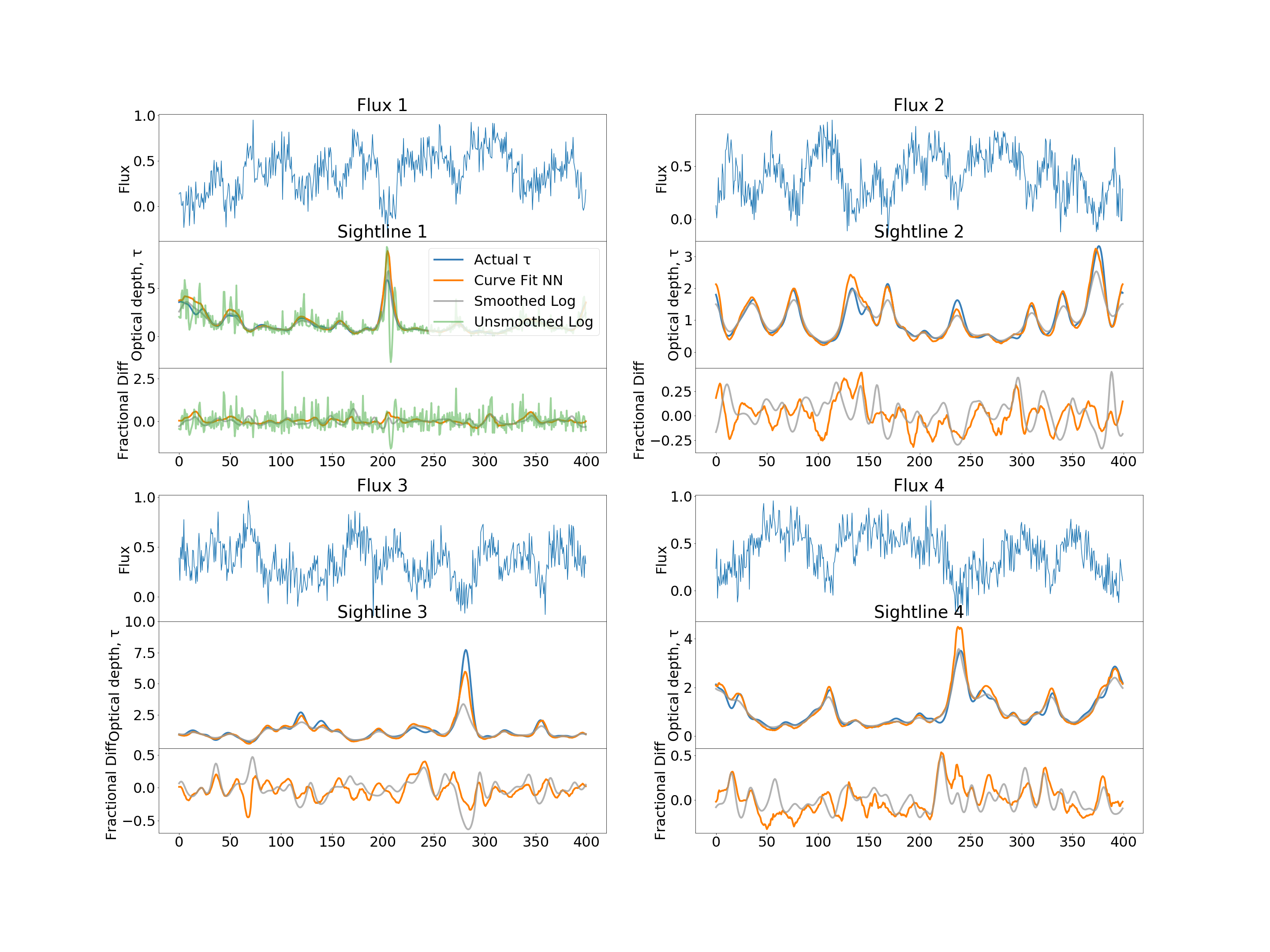
Figure 3: Ly$\alpha$ optical depth $\tau$ predicted by the curve fit NN (detailed in Section 4.2) for four example sightlines. We also show results for alternative reconstruction methods involving taking the log and interpolating with cubic splines (see Section 3.5). In addition, we show the fractional difference between predicted $\tau$ and real $\tau$ for each method beneath the reconstructions. We first calculate flux, then add noise with a signal-to-noise ratio of 5 before using the four different reconstruction methods to predict $\tau$. The $x$-axis units are comoving $h^{-1}{\rm Mpc}$

3 Method: Deep learning reconstruction of the Lyman-$\alpha$ forest

3.1 Data preprocessing

As explained in Section 1, we train a NN using our mock datasets, and use it to recover the optical depth to Ly$\alpha$ absorption, $\tau$, from input values of flux $F$.

The data are split into training, test, and validation sets (the role of each will be explained in Section 3.4 below). 60% of the sightlines are assigned to the training set, and 20% each to the validation and testing sets. The sightlines are arranged in a 2D array, where nearby sightlines are strongly correlated with each other. The sightlines that make up the validation and test sets come from opposite corners of the 2D array to ensure the test and validation sets are as independent as possible from the training data.

As mentioned above, we generate Gaussian noise at three different signal-to-noise ratios. While we generate new noise at every epoch for the training data, we create and save the noise for the validation and test sets for more consistent evaluation of the neural network and comparison to other reconstruction methods.

For each sightline, the data used for training are the mock observational datasets consisting of $F$ values, to which noise has been applied, and the optical depth $\tau$ values. The latter represent the underlying physical quantities which the NN will learn how to derive from the former. Because we are primarily interested in the large scale structure of the forest, we smooth the $\tau$ values as part of our data preprocessing before passing them to the NN for training (the training flux values are unsmoothed). The smoothing is done with a Gaussian kernel of $\sigma$ equal to six pixels (4.7 $h^{-1}{\rm Mpc}$).

3.2 Neural network

Convolutional neural networks (CNNs) have revolutionized the field of computer vision in the last decade achieving state-of-the-art performance on almost all computer vision tasks, such as image classification, object detection and semantic segmentation (Rawat & Wang, 2017). CNNs provide the ability to solve non-linear inversion problems by learning spatial features that are invariant to translation and local distortions. Consequently they are being increasingly used in various fields other than computer vision including cosmology (Ribli et al., 2019; Ravanbakhsh et al., 2017). Hence we choose to use a convolution neural network architecture to learn spatial features from flux input to predict optical depth, and the proposed architecture is displayed in Figure 2. The inputs are the observed flux values, $F$, for the 512 pixels in the same sightline. The output is the prediction for the optical depth $\tau$ at the center pixel of a sightline (which we take to be the 256th out of the 512 pixels). To predict $\tau$ values for other pixels in the sightline, we shift the pixels such that the position of output pixel is at the center of the sightline. Each sightline can therefore be used for training 512 times, each time with a different pixel at the center. The periodic boundary conditions of the simulation are respected during this process.

In Figure 2, we can see the different layers that the input is processed through. The first, (a) is a convolutional layer with kernel size of 5 pixels and stride of 1 pixel. This layer has 4 filters which it applies to the sightline, producing four-channel data from the originally one dimensional data. The next, layer (b) is a max pool layer: for discrete sets of five neighboring pixels, the layer outputs the maximum value using a stride of 1 pixel. This is done for each of the four channels individually. Layers (c), (d), and (e) are fully connected linear layers with decreasing numbers of outputs. Prior to layer (e), the array is flattened so that the final layer returns a single output. The outputs of layers (a), (c), and (d) pass through the Rectified Linear Unit (ReLU) activation function, $f(x)=max(0,x)$. The final architecture and hyperparameters are chosen by experimentation using the validation dataset which is described in the following section 3.3.

As the NN is trained, the weights are adjusted based on minimization of a loss function. We use the mean squared error (MSE) as the loss function:

$$L(\hat{\tau},\tau)=\frac{1}{n}\sum_{n}(\hat{\tau}-\tau)^{2}$$ (3)

Here, $\tau$ is the actual $\tau$ value in a pixel and $\hat{\tau}$ is the neural network prediction for $\tau$, while $n$ is the batch size. The adjustment of weights is carried out using Adam optimizer (Kingma & Ba, 2014), an efficient alternative to the standard stochastic gradient descent method. We also use L2 regularization, which adds a regularization term to the loss function. The goal is to decrease the network complexity and improve generalization. For L2 regulation, we use the decoupled weight decay regularization method (Loshchilov & Hutter, 2017) that is part of the Adam optimizer implementation within the PYTORCH library (Paszke et al., 2019). We set the weight decay parameter in L2 regularization to $5*10^{-4}$. The neural network is trained on 10,000 samples every epoch. The code base was written using the PYTORCH library, and we make it publicly available to the research community.

3.3 Hyperparameters

We choose our proposed neural network architecture after training and evaluating various architectures across a range of hyperparameters on the validation set. We initially experiment with fully connected network architectures with varying numbers of hidden layers and units, but we find that it does not learn. Hence we switch to use convolutional neural network (CNN) architectures as motivated in the previous section. For the CNN architecture, we experiment with different kernel sizes between 3 to 5, output channels between 2 to 4, and linear layers between 2 to 5 to find the optimal architecture. For each of the architectures, we experiment with a range of learning rates between $10^{-3}$ and $10^{-6}$ for thorough comparison. Ultimately, we find that our proposed architecture described in Figure 2 results in the most accurate predictions.

Additionally, we experiment with different types of pooling layers including max, min and average pooling layers. Pooling is often performed after convolutional layers in order to reduce the spatial resolution of the feature maps and thus achieve spatial invariance to input distortions and translations. As we use a kernel size of 5, max pooling separates the data into groups of 5 consecutive pixels. For each of these groups, the maximum value within the consecutive pixels is taken as the output value for the group. Similarly, min pooling does the same using the minimum value, while average pooling takes the arithmetic average of the 5 pixel group. Some works (Scherer et al., 2010; Jarrett et al., 2009) have empirically shown that max pooling provides superior generalization and faster convergence leading to most state-of-the-art architectures using max pooling. However, another work (Boureau et al., 2010) focuses on theoretical analysis of max pooling and average pooling supplemented by empirical evaluations to conclude that the performance of either max or average pooling depends on the data and its features. Hence we conduct experimental analysis to evaluate the optimal pooling layer type for our dataset and architecture. We find that min and average pooling perform marginally better (within 3 standard deviations of Root Mean Squared Error, RMSE) for $\tau<2$, but perform marginally worse (within 1 standard deviation) on higher values, $\tau>2$, as compared to max pooling. Since the performance across different pooling layers is comparable for our dataset, we choose max pooling in our proposed architecture as it performs marginally better on the high $\tau$ values, which is the region of saturated flux data we are interested in. The details of RMSE and standard deviation calculation are provided in Section 4.3.

We report the neural network’s hyperparameters here for completeness. We use a learning rate of $10^{-4}$, batch size of 10,000, and train for 50,000 epochs. We use Adam optimizer, as implemented in the PYTORCH library, with betas equal to (0.9, 0.999), eps of $10^{-8}$, and weight_decay of $5*10^{-4}$.

3.4 Training

In training, we randomly select 10,000 pixels from our training set, shifting their sightlines so that the selected pixel is at the center. We then add noise to the $F$ values. As explained in Section 2.2, we use a normal distribution for noise, with standard deviation determined by the desired signal-to-noise ratio. The NNs are both trained and tested at a single signal-to-noise ratio. We do find, however that a NN trained using data with a S/N of 5 still outperforms comparison reconstruction methods at other signal to noise ratios (namely 2.5 and 10). We discuss further on this in Section 5.2. The validation dataset is used to evaluate performance of the neural network and tune hyperparameters, while the test dataset is used for final results.

3.5 Comparison methods for reconstruction

It will be useful to compare the NN reconstruction of $\tau$ from noisy $F$ values with other reconstruction methods. Looking at Equation 1, one can see that the simplest method would be a straight inversion, $\tau=-\ln{F}$. This is the first alternative reconstruction method that we try. Of course it is necessary in this case to deal with negative values of $F$. We do this using cubic spline interpolation. When a pixel $F$ value is negative, we initially ignore it, calculating the negative log of all positive $F$ values while saving their positions on the sightline. Once all positive $F$ values have a predicted $\tau$, we then use cubic spline interpolation with a periodic boundary to estimate $\tau$ for pixels with negative $F$.

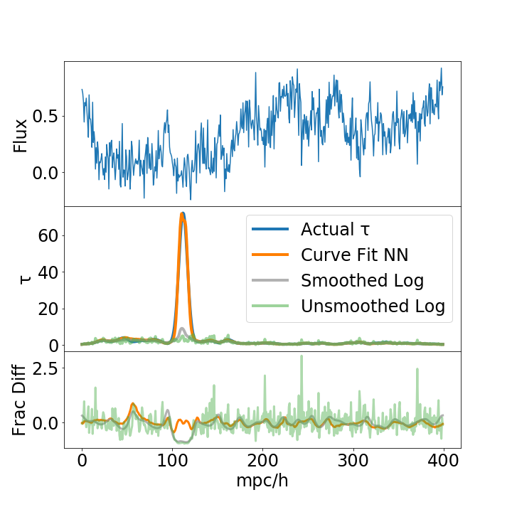
Figure 4: Reconstruction of a sightline with high values of $\tau$. This sightline was selected for having the most pixels with $\tau$ greater than 50. See the caption of Figure 3 for more details.

Our second comparison method (which gives better results) involves first smoothing the $F$ values with a Gaussian kernel with a $\sigma$ of 6 pixels, and then computing $\tau=-\ln{F}$. We label this method Smoothed Input Log. In this case, there are fewer negative pixel values, but when there are, we again use cubic spline interpolation, as in the previous method.

Figure 5: Reconstruction of the same sightline for three different noise levels. See the caption of Figure 3 for more details.

4 Results

After training the NN for 50,000 epochs using the training data, and adjusting the hyperparameters using the validation dataset, we apply the NN reconstruction to the test dataset (which consists of 20% of the sightlines). In this section we show some example sightlines as well as some statistical evaluations of the fidelity of the reconstructions.

Figure 6: Scatter plots of the reconstruction predictions for the Ly$\alpha$ optical depth $\tau$ as a function of the true $\tau$ in each pixel. Each panel shows a different reconstruction technique. Clockwise from top left these are, (a) NN prediction; (b) Log inversion of the unsmoothed $F$ data, including cubic spline interpolation; (c) Log inversion of the smoothed $F$ data, including cubic spline interpolation; and (d) NN prediction adjusted with curve fit to high $\tau$ pixels. The line in black shows the median prediction for each bin of the real tau value. The right subfigure shows the same scatter plots as the left, but with log scaling in the axes.

4.1 Example sightlines

In Figure 3 we show results for four randomly chosen sightlines. We show the input noisy $F$ values as a function of distance along the sightline in the top panel in each case. All of the examples in this plot are for an input spectra with S/N = 5. Underneath the $F$ panel in each case, we show the actual $\tau$ values, as well as the results of the curve fit NN reconstruction (detailed in Section 4.2), and the Smoothed Input Log inversion. For only one of the panels (the top left) we show the results of the direct log inversion (”Unsmoothed Log”, in green), but do not show it in the others because it obscures the other results. We also show the fractional difference between predicted $\tau$ and real $\tau$ for each method beneath the reconstructions. The fractional difference is calculated as $(\tau_{pred}-\tau_{real})/\tau_{real}$.

We can see that the NN has learned to reconstruct the $\tau$ curve from the noisy flux quite well. The general nature of the fluctuations is reproduced, even in regions where the $F$ values become significantly negative due to noise. The Smoothed Input Log reconstruction also works reasonably well, although appears to underpredict in the high $\tau$ regions.

In Figure 4, we show the situation for a sightline with very high $\tau$ values, again with S/N = 5. This sightline was chosen because it had the most pixels with $\tau>50$. We can see that there is a significant region, about $100h^{-1}{\rm Mpc}$ in width, where the flux values are roughly consistent with zero given the noise. The direct inversion method shown in green does not capture any of the high $\tau$ structure in this region. The Smoothed Log method does find a bump with $\tau\sim 10$ in the right place, but the NN is able to use the information on $F$ surrounding the high $\tau$ pixels to reconstruct a reasonable likeness of the ”hidden” $\tau$ in the most absorbed region.

The previous plots showed results for a moderate noise level, S/N=5. In Figure 5 we show the flux and the $\tau$ predictions across the different levels of noise we have tried, where the S/N values are equal to 2.5, 5, and 10. In this case, we show the same sightline in each case, only the noise being different. We do not show the Unsmoothed Log reconstruction to avoid obscuring the other lines. We can see that there are significant differences in the small scale structure of $\tau$ reconstructed by both the NN and the Smoothed Log in the low S/N case, although both recover the largest peak quite well. As the S/N increases, the fidelity becomes markedly better, with the largest qualitative improvement between S/N=2.5 and S/N=5. The statistical evaluation of the accuracy of this method for different S/N is carried out in the Section 4.3.

4.2 Scatter plots

We now move to comparisons of results from all pixels. We show scatter plots of the $\tau$ predictions from the NN and other reconstruction methods vs the true $\tau$ values in Figure 6.

The NN prediction is in the top left panel, and we can see that the $y=x$ line appears to pass through the center of the point cloud for $\tau$ values below 10. We see however that the NN prediction appears to be non-linear for $\tau$ values that are higher than this. For example, the $\tau$ prediction never rises above $\tau=16$, although there are pixels in the spectra which have higher $\tau$ values.

The neural network likely has difficulty predicting high $\tau$ for two reasons. Pixels with high $\tau$ values will have a low flux, so any added noise can have a large impact. The second reason is due to a class imbalance problem (Buda et al., 2018), as pixels of high $\tau$ are rarer than pixels of low $\tau$, with only 0.01% of pixels being above $\tau=20$. We attempt to deal with the class imbalance problem by adjusting the loss function to evaluate loss differently for higher values of $\tau$. We divide pixels into 3 bins; $\tau<2$, $2\leq\tau<30$, and $\tau\geq 30$. We calculate the proportion of pixels in each bin then take the weighted average of square errors:

$$L(\hat{\tau},\tau)=\frac{1}{n}\bigg{(}\sum_{\tau<2}\frac{(\hat{\tau}-\tau)^{2}}{b_{1}}+\sum_{2\leq\tau<30}\frac{(\hat{\tau}-\tau)^{2}}{b_{2}}+\sum_{\tau\geq 30}\frac{(\hat{\tau}-\tau)^{2}}{b_{3}}\bigg{)}$$ (4)

Where $b_{i}$ refers to the proportion of pixels in the entire training set that are in each bin and n is the batch size, which we chose to be 10,000. The numerical values for the bin proportions are as follows; $b_{1}=0.906,b_{2}=0.094,b_{3}=2.12*10^{-5}$.

With this method, we increase the loss in bins of high $\tau$ according to the proportion of pixels in each bin. This method was unsuccessful in increasing accuracy, with a RMSE value of 0.533 at a signal-to-noise ratio of 5, which was 25% higher than using mean square error as the loss function. We also attempted using two neural networks to predict one sightline, with one network predicting low values of $\tau$ and the other predicting high values of $\tau$. These models’ architectures are the same architecture we use in this paper. This method was also unsuccessful in increasing accuracy.

Another possibility is to directly address the class imbalance problem by training the network on sightlines from a range of redshifts so that the network has more training data with high $\tau$ values. We leave exploring this method to future work.

Even though the number of extremely high $\tau$ pixels is small (only 1.16% of pixels have true $\tau>10$), in order to achieve higher accuracy, we use a curve fitting algorithm on the ratio of actual $\tau$ to predicted $\tau$ where the actual $\tau$ is greater than or equal to 2. For these datapoints, we use the actual to prediction ratio as our y-values and the actual $\tau$ as our x-values. By fitting a curve to these points, we construct a function of actual $\tau$ that outputs the ratio between actual $\tau$ and predicted $\tau$. In order to correct our neural network predictions, we multiply each point in the scatterplot by the ratio given by the function and the actual $\tau$ value of the pixel.

When fitting a cubic function to these ratios, we find parameters that minimize the residuals between the cubic function and these datapoints using the Levenberg-Marquadt optimization algorithm. The resulting cubic function is $r=-0.000078\cdot x^{3}+0.0046\cdot x^{2}+0.047\cdot x+0.81$, where r is the ratio between actual $\tau$ and predicted $\tau$. Because the neural network’s prediction is linear for low $\tau$, we don’t modify those points. In future work, we will investigate whether the NN can be trained to do better on the highest $\tau$ points, but do not do this here, in order to keep the NN part of our algorithm simple.

The result of including a curve fit to the predictions is shown in the ”Curve Fit Neural Network Prediction” panel in Figures 6. We do not apply the same method to the analytical method Smoothed Input Log because its prediction at the highest $\tau$ values is approximately symmetric about $y=x$, and we find that curve fitting would not increase accuracy significantly.

The results from the Smoothed Input Log reconstruction are in the bottom right panel of Figure 6. We can see both that the scatter extends significantly wider than for the NN method, and that there is curvature in the mean relation even for values as low as $\tau\sim 3$. As mentioned above, for higher $\tau$ values (above $\tau=15$) there is not evidence for curvature but the scatter is extremely high. The Unsmoothed Log Prediction (top right panel) is not biased at low $\tau$, but has visually much worse scatter.

4.3 Statistical measures

We have seen that the neural network appears to qualitatively outperform our alternative reconstruction methods, and have seen some examples of sightlines with different levels of signal to noise. We now evaluate the performance quantitatively, by comparing the reconstructed $\tau$ values in sightlines to the true $\tau$ values. Again, the results are from predictions on the test set, which the neural network has not trained on. One measure of the accuracy of the reconstruction is the Root Mean Squared Error, RMSE, defined as

$${\rm RMSE}=\sqrt{\frac{1}{n}\sum_{i=1}^{n}(\hat{\tau_{i}}-\tau_{i})^{2}},$$ (5)

where the sum is over the $n$ pixels in the test dataset, $\hat{\tau_{i}}$ is the reconstructed optical depth in pixel $i$ and $\tau_{i}$ is the true value.

Our second measure of the accuracy is the fractional error, which we define to be RMSE$/{\overline{\tau}}$, where ${\overline{\tau}}$ is the mean optical depth for the particular dataset being evaluated. The different datasets are either the full range of pixels in spectra, or the high $\tau$ pixels (with $\tau>2$), or those with low $\tau$ ($\tau<2$) Across the entire data set, mean ${\overline{\tau}}$ is 1.107. For $\tau<2$, mean ${\overline{\tau}}=0.543$, and for $\tau\geq 2$, ${\overline{\tau}}=5.468$.

There are three levels of stochasticity to the RMSE values. The first comes from the noise, the second comes from the initial weights of the neural network, and the third comes from the source of our sightlines. In order to capture two of the three levels of stochasticity, the RMSE values in Tables 1, 2, and 3 are the averages of 7 neural networks with different initial weights predicting $\tau$ with different generated noise. The comparison reconstruction RMSE values are also an average over 7 different sets of randomly generated noise. The standard deviations are calculated from the seven different reconstructions in each category using the following formula:

$$\sigma=\frac{\sqrt{\sum(x-\bar{x})^{2}}}{n-1}$$ (6)

Here, $x$ is the RMSE value, $\bar{x}$ is the average RMSE value for the reconstruction method at a given signal-to-noise ratio and $\tau$ range, and n is the number of samples, which is 7 here.

Table 1: RMSE of our neural network’s prediction vs log prediction over our test set, with a signal-to-noise ratio of 10. The RMSE is split into three sections, where we calculate RMSE for the total test dataset, just for high values of $\tau$, and just for low values. We define $\tau\geq 2$ to be a high value of $\tau$.

Name	RMSE${}_{\text{total}}$	RMSE${}_{\text{high}}$	RMSE${}_{\text{low}}$
Curve Fit NN	0.285 $\pm$ 0.01	0.882 $\pm$ 0.05	0.091 $\pm$ 0.02
Neural Network	0.330 $\pm$ 0.01	1.036 $\pm$ 0.03	0.091 $\pm$ 0.02
Log	0.620 $\pm$ $7\mathrm{e}{-4}$	1.908 $\pm$ $2\mathrm{e}{-3}$	0.214 $\pm$ $2\mathrm{e}{-4}$
Smooth Input Log	0.511 $\pm$ $2\mathrm{e}{-3}$	1.620 $\pm$ $8\mathrm{e}{-3}$	0.124 $\pm$ $5\mathrm{e}{-5}$

Table 2: RMSE values for SNR of 5 (see Table 1 caption for details)

Name	RMSE${}_{\text{total}}$	RMSE${}_{\text{high}}$	RMSE${}_{\text{low}}$
Curve Fit NN	0.342 $\pm$ $4\mathrm{e}{-3}$	1.012 $\pm$ 0.01	0.151 $\pm$ $8\mathrm{e}{-3}$
Neural Network	0.423 $\pm$ $3\mathrm{e}{-3}$	1.296 $\pm$ 0.01	0.151 $\pm$ $8\mathrm{e}{-3}$
Log	0.800 $\pm$ $1\mathrm{e}{-3}$	2.192 $\pm$ $4\mathrm{e}{-3}$	0.455 $\pm$ $3\mathrm{e}{-4}$
Smooth Input Log	0.538 $\pm$ $4\mathrm{e}{-3}$	1.696 $\pm$ 0.01	0.141 $\pm$ $4\mathrm{e}{-4}$

Table 3: RMSE values for SNR of 2.5 (see Table 1 caption for details)

Name	RMSE${}_{\text{total}}$	RMSE${}_{\text{high}}$	RMSE${}_{\text{low}}$
Curve Fit NN	0.430 $\pm$ $7\mathrm{e}{-3}$	1.044 $\pm$ 0.08	0.299 $\pm$ 0.03
Neural Network	0.560 $\pm$ $8\mathrm{e}{-3}$	1.570 $\pm$ 0.03	0.299 $\pm$ 0.03
Log	1.076 $\pm$ $8\mathrm{e}{-4}$	2.529 $\pm$ $3\mathrm{e}{-3}$	0.782 $\pm$ $4\mathrm{e}{-4}$
Smooth Input Log	0.674 $\pm$ $7\mathrm{e}{-3}$	2.100 $\pm$ 0.02	0.208 $\pm$ $1\mathrm{e}{-3}$

(a) RMSE

(b) Fractional Error

Figure 7: RMSE and Fractional Error for different methods across different noise levels, separated further into three groups; all $\tau$ values; only high $\tau$ values; and only low $\tau$ values. The four methods are neural network prediction, curve fit neural network prediction (where the output is fit onto $y=x$), log prediction, and smoothed input log prediction (where the input flux is smoothed with a Gaussian kernel size of 6 pixels). The RMSE is calculated using Equation 5. The fractional error is defined to be RMSE divided by mean $\tau$ in each group.

We present our results in Tables 1-3 and in graphical form in Figures 7(a) and 7(b). A quick glance reveals that in these figures that the blue bar, the NN adjusted by curve fitting has the lowest RMSE and Fractional error in all cases, except for the $\tau<2$ results for S/N of 2.5 and 5. The improvement over the raw log transformation is significant for the total of all pixels, and for $\tau<2$, varying from a factor of 2.1 to 2.5, with no variation for different S/N. If we compare instead to the smoothed input log reconstruction, we find that that the curve fit neural network improves the reconstruction by a factor of between 1.6 and 2.0 for all and high $\tau$ pixels.

The curve fitting addition to the NN makes the most difference for low S/N and high $\tau$ pixels. There is no difference for $\tau<2$. The improvement over the NN on its own varies from a factor of 1.1 to 1.5. Apart from the $\tau<2$ low S/N results mentioned above, the NN without curve fitting is significantly better than the smoothed input log reconstruction. When considering the accuracy on a pixel by pixel basis, the fractional error (Figure 7(b)) is useful. We can see that we can aspire to a fractional error on $\tau$ reconstruction for $\tau>2$ using the curve fit NN of less than 20%, for all S/N levels tested.

5 Summary and discussion

5.1 Summary

We have set up a neural network to train on 1D Ly$\alpha$ forest datasets from simulations.The aim is to use the trained NN to recover underlying Ly$\alpha$ optical depth values from noisy and saturated transmitted flux data in quasar spectra. The NN has an architecture which includes both convolutional and fully connected layers. We have trained the network using spectra from hydrodynamic simulations of a CDM cosmology. The NN has been applied to a test dataset, and its accuracy evaluated statistically using the root mean square difference between the reconstructed and true $\tau$ values in the simulation. We have compared the NN reconstruction to straightforward logarithmic inversion of the noisy flux data (including spline interpolation of $\tau$ through saturated regions) and also logarithmic inversion of the smoothed flux data. Our findings are as follows:

• The curve fit neural network is at least twice as accurate as the naive log reconstruction method.

• Curve fitting decreased the neural network’s RMSE by 15% on average.

• The curve fit neural network outperforms all the other methods except the Smoothed Input Log method for low values of $\tau$ ($\tau$ ¡ 2) where the signal-to-noise ratio is 2.5 or 5.

5.2 Discussion

Although we have concentrated on the simplest task in this paper, inversion of Equation 1 for noisy and saturated data, it should be relatively straightforward in principle to apply the same techniques to reconstruct other quantities from the transmitted Ly$\alpha$  forest flux, $F$. The simulations include information on the underlying physical quantities relevant to $F$, such as the baryonic and dark matter density, temperature and velocity fields. We leave testing such reconstructions to future work, but we note that some quantities such as the velocity field may be difficult to infer from individual 1D sightlines, as they are generated by the matter distribution in three dimensional space. It will nevertheless be interesting to see how much can be recovered from one dimension only. All reconstructed quantities will of course be dependent on the simulations and model used for training the NN (we return to this below). For example, little direct information on the gas temperature is available from the low resolution spectra we have considered so far (thermal broadening occurs on too small a scale), but a NN would presumably recover a physically reasonable but very model dependent temperature indirectly from the relationship between temperature and density in the IGM (Hui & Gnedin 1997). Recent work on a similar theme, but in three dimensions is that of Hong et al. (2020) who have used hydrodynamic simulations of galaxy formation to train a NN to reconstruct the dark matter distribution from galaxy positions and velocities.

Having only trained our NN on one simulation, the answers that it returns are likely to be strongly dependent on that training set. We have carried out tests using mock data with different S/N ratios (training with a different S/N than the test data), and find reasonable results, but it would be very interesting in future work to try training the NN with data from different redshifts or cosmologies from the test data.

Another issue related to the finite size of the training dataset is that there will be rare events which could be underrepresented, such as large fluctuations in the optical depth. There will also be features in real data which are not included in the simulations, depending on their level of sophistication. For example we have not included damped Ly$\alpha$  lines in our mock datasets, or metal lines. In principle these could be added to training data, as simulations exist which make predictions for them (e.g., Pontzen et al. 2008). The physics involved (including galaxy and star formation) is however more uncertain and less likely to resolved in the simulations than the physics leading to the majority of the Ly$\alpha$ optical depth.

We have compared the NN reconstruction method with two other methods for inferring the optical depth from the flux. It is of course possible that other methods could be imagined which have better performance. For example, in one method, we smooth the flux before log inversion and spline interpolation. One could imagine using some more sophisticated denoising such as L1 trend filtering (Politsch et al., 2020a, b) before log inversion. Physical reconstruction modeling could also be tried, which uses the physics of the intergalactic medium in simulations to go from flux to physical quantities. Examples include Nusser & Haehnelt (1999), and Müller et al. (2020). Other machine learning techniques have been applied to similar problems in absorption line data, for example use of a genetic algorithm to model data with multiple metal line species (Lee et al. 2020), or the use of conditional neural spline flows to predict the quasar continuum on the red side of the quasar Ly$\alpha$  line from blue side data (Reiman et al., 2020).

Our particular NN approach works better than the alternatives we have tested, except for the highest optical depth regions $\tau\lower 2.15277pt\hbox{$\;\buildrel>\over{\sim}\;$}15$, where the scatter is low but there is a bias. These correspond to an extremely small percentage of pixels, but nevertheless it would be very useful to improve the NN there. We have investigated changes in NN hyperparameters, but have not been able to simply improve the NN performance in these regions. We have instead adopted a curve fit approach to the highest $\tau$ pixels, which, like the NN uses information from the simulations. The combined NN and curve fit approach does yield good results at high $\tau$, making use of the fact that the NN is able to reduce the scatter even though its results are biased. We leave a comprehensive effort to improve the NN in these regions to future work.

Another open question is how the NN is making its predictions for $\tau$. The flux in an entire simulated spectrum (spanning 512 pixels and 400 $h^{-1}{\rm Mpc}$) is used by the NN as an input. In future work, we plan to investigate the response of the NN and how it is using the input information, for example weighted by pixel distance. The log inversion techniques use only single pixel information in unsaturated regions, but signal over longer distances in the spline interpolation part of the algorithms. It will be interesting to compare the dependence of the NN algorithm on distance of the farthest data used from the predicted pixel.

We have approached this paper from the point of view that solving the inverse problem (in this example of observed flux to underlying optical depth) is an interesting intellectual exercise. One should obviously also ask however how useful our DL solution actually is, what its limitations might be. Different use cases can be imagined, but they will likely all be dependent on the model used in training, unless significant testing (for example with different simulations) shows how more general conclusions can be inferred. We indulge in a limited amount of speculation here. If we are testing a particular model (for example $\Lambda$CDM with specific parameters), we could use simulations of that model for training and then compare statistics of the reconstructed fields (e.g., temperature, density) to see if they are consistent with the original model. This would allow testing using statistical measurements of quantities which are not directly observable. In the case of Ly$\alpha$ optical depth $\tau$ studied in this paper, we could imagine measuring the clustering of $\tau$, including perhaps higher order statistics. Whether these would actually have more discriminatory power than statistics of measurable quantities such as the flux $F$ is debatable, but at the very least they may offer different ways of weighting the data (see McCullagh et al. 2016 and related works for other approaches). For example the S/N of Ly$\alpha$ BAO measurements may improve (or not) if the observations are transformed to a $\tau$ field or a density field first.

Certainly, in the case of the Ly$\alpha$ forest there is increasing interest in the use of interpolation techniques to construct three dimensional maps from arrays of one dimensional spectra (Pichon et al., 2001; Horowitz et al., 2019; Newman et al., 2020)). Instead of producing a 3D flux field, one could use the NN reconstruction to make 3D $\tau$, temperature, or density fields. One use of reconstructed sightlines or maps could be to use in cross-correlation with other data. The Ly$\alpha$  forest has a low bias factor (the ratio of $F$ fluctuations to matter fluctuations), with $|b|\sim 0.2$ (Slosar et al., 2011), and transforming to a variable with a higher $|b|$ such as $\tau$ could increase the S/N of Ly$\alpha$  forest - Ly$\alpha$  emission cross-correlations (e.g., Croft et al. 2018), for example. Because the DL reconstruction appears to work significantly better on noisy data than smoothing does, one could imagine using it to remove noise artifacts, or perhaps even set the unobserved quasar continuum level (by training on mock data with varied continua).

We have seen that NN are able to learn the relationships between complex physical quantities in simulations. In the case of the Ly$\alpha$ forest this can be used to carry out model dependent reconstruction from observables. As with many applications of Artificial Intelligence techniques, the uses and limitations are not all yet apparent, but it is obvious that there is much of promise that should be studied further.

Acknowledgments

RACC is supported by NASA ATP 80NSSC18K101, NASA ATP NNX17AK56G, NSF NSF AST-1909193, and a Lyle Fellowship from the University of Melbourne. This work was also supported by the NSF AI Institute: Physics of the Future, NSF PHY- 2020295. We would like to thank the referee for their comments and suggestions for future work.

5.3 Data availability

The data underlying this article are accessible through the code repository..

References

- Aubourg et al. (2015) Aubourg É., et al., 2015, Phys. Rev. D, 92, 123516
- Bi (1993) Bi H., 1993, ApJ, 405, 479
- Boureau et al. (2010) Boureau Y., Ponce J., LeCun Y., 2010
- Buda et al. (2018) Buda M., Maki A., Mazurowski M. A., 2018, Neural Networks, 106, 249
- Caldeira et al. (2019) Caldeira J., Wu W. L. K., Nord B., Avestruz C., Trivedi S., Story K. T., 2019, Astronomy and Computing, 28, 100307
- Cen et al. (1994) Cen R., Miralda-Escudé J., Ostriker J. P., Rauch M., 1994, ApJ, 437, L9
- Charnock et al. (2018) Charnock T., Lavaux G., Wandelt B. D., 2018, Phys. Rev. D, 97, 083004
- Cheng et al. (2020) Cheng T.-Y., et al., 2020, MNRAS, 493, 4209
- Cisewski et al. (2014) Cisewski J., Croft R. A. C., Freeman P. E., Genovese C. R., Khandai N., Ozbek M., Wasserman L., 2014, MNRAS, 440, 2599
- Croft et al. (2018) Croft R. A. C., Miralda-Escudé J., Zheng Z., Blomqvist M., Pieri M., 2018, MNRAS, 481, 1320
- Di Matteo et al. (2012) Di Matteo T., Khandai N., DeGraf C., Feng Y., Croft R. A. C., Lopez J., Springel V., 2012, ApJ, 745, L29
- Dodelson (2003) Dodelson S., 2003, Modern cosmology
- Fluri et al. (2019) Fluri J., Kacprzak T., Lucchi A., Refregier A., Amara A., Hofmann T., Schneider A., 2019, Phys. Rev. D, 100, 063514
- George & Huerta (2018) George D., Huerta E. A., 2018, Physics Letters B, 778, 64
- Goodfellow et al. (2016) Goodfellow I. J., Bengio Y., Courville A., 2016, Deep Learning. MIT Press, Cambridge, MA, USA
- Gunn & Peterson (1965) Gunn J. E., Peterson B. A., 1965, ApJ, 142, 1633
- Haardt & Madau (1996) Haardt F., Madau P., 1996, ApJ, 461, 20
- He et al. (2019) He S., Li Y., Feng Y., Ho S., Ravanbakhsh S., Chen W., Póczos B., 2019, Proceedings of the National Academy of Science, 116, 13825
- Hernquist et al. (1996) Hernquist L., Katz N., Weinberg D. H., Miralda-Escudé J., 1996, ApJ, 457, L51
- Hong et al. (2020) Hong S. E., Jeong D., Hwang H. S., Kim J., 2020, arXiv e-prints, p. arXiv:2008.01738
- Horowitz et al. (2019) Horowitz B., Lee K.-G., White M., Krolewski A., Ata M., 2019, ApJ, 887, 61
- Hui & Gnedin (1997) Hui L., Gnedin N. Y., 1997, MNRAS, 292, 27
- Jarrett et al. (2009) Jarrett K., Kavukcuoglu K., Ranzato M., LeCun Y., 2009, in 2009 IEEE 12th international conference on computer vision. pp 2146–2153
- Kingma & Ba (2014) Kingma D. P., Ba J., 2014, Adam: A Method for Stochastic Optimization (arXiv:1412.6980)
- Kodi Ramanah et al. (2020) Kodi Ramanah D., Charnock T., Villaescusa-Navarro F., Wandelt B. D., 2020, MNRAS, 495, 4227
- LeCun et al. (2015) LeCun Y., Bengio Y., Hinton G., 2015, Nature, 521, 436
- Lee et al. (2013) Lee K.-G., et al., 2013, AJ, 145, 69
- Lee et al. (2020) Lee C.-C., Webb J. K., Carswell R. F., Milakovic D., 2020, arXiv e-prints, p. arXiv:2008.02583
- Li et al. (2020) Li Y., Ni Y., Croft R. A. C., Di Matteo T., Bird S., Feng Y., 2020, arXiv e-prints, p. arXiv:2010.06608
- López et al. (2016) López S., et al., 2016, A&A, 594, A91
- Loshchilov & Hutter (2017) Loshchilov I., Hutter F., 2017, Decoupled Weight Decay Regularization (arXiv:1711.05101)
- Lucie-Smith et al. (2018) Lucie-Smith L., Peiris H. V., Pontzen A., Lochner M., 2018, MNRAS, 479, 3405
- McCullagh et al. (2016) McCullagh N., Neyrinck M., Norberg P., Cole S., 2016, Monthly Notices of the Royal Astronomical Society, 457, 3652
- Metcalf et al. (2019) Metcalf R. B., et al., 2019, A&A, 625, A119
- Mitchell (1997) Mitchell T., 1997, Machine Learning. McGraw Hill
- Müller et al. (2020) Müller H., Behrens C., Marsh D. J. E., 2020, MNRAS,
- Muthukrishna et al. (2019) Muthukrishna D., Parkinson D., Tucker B. E., 2019, ApJ, 885, 85
- Newman et al. (2020) Newman A. B., et al., 2020, ApJ, 891, 147
- Nusser & Haehnelt (1999) Nusser A., Haehnelt M., 1999, MNRAS, 303, 179
- Parks et al. (2018) Parks D., Prochaska J. X., Dong S., Cai Z., 2018, MNRAS, 476, 1151
- Paszke et al. (2019) Paszke A., et al., 2019, in Wallach H., Larochelle H., Beygelzimer A., d'Alché-Buc F., Fox E., Garnett R., eds, , Advances in Neural Information Processing Systems 32. Curran Associates, Inc., pp 8024–8035, http://papers.neurips.cc/paper/9015-pytorch-an-imperative-style-high-performance-deep-learning-library.pdf
- Pichon et al. (2001) Pichon C., Vergely J. L., Rollinde E., Colombi S., Petitjean P., 2001, MNRAS, 326, 597
- Politsch et al. (2020a) Politsch C. A., Cisewski-Kehe J., Croft R. A. C., Wasserman L., 2020a, MNRAS, 492, 4005
- Politsch et al. (2020b) Politsch C. A., Cisewski-Kehe J., Croft R. A. C., Wasserman L., 2020b, MNRAS, 492, 4019
- Pontzen et al. (2008) Pontzen A., et al., 2008, MNRAS, 390, 1349
- Rauch (1998) Rauch M., 1998, ARA&A, 36, 267
- Ravanbakhsh et al. (2017) Ravanbakhsh S., Oliva J., Fromenteau S., Price L. C., Ho S., Schneider J., Poczos B., 2017, Estimating Cosmological Parameters from the Dark Matter Distribution (arXiv:1711.02033)
- Rawat & Wang (2017) Rawat W., Wang Z., 2017, Neural computation, 29, 2352
- Reiman et al. (2020) Reiman D. M., Tamanas J., Prochaska J. X., Ďurovčíková D., 2020, arXiv e-prints, p. arXiv:2006.00615
- Ribli et al. (2019) Ribli D., Pataki B. Á., Zorrilla Matilla J. M., Hsu D., Haiman Z., Csabai I., 2019, Monthly Notices of the Royal Astronomical Society, 490, 1843
- Russell & Norvig (2020) Russell S. J., Norvig P., 2020, Artificial Intelligence: a modern approach, 4 edn. Pearson
- Savaglio et al. (2002) Savaglio S., Panagia N., Padovani P., 2002, ApJ, 567, 702
- Schawinski et al. (2017) Schawinski K., Zhang C., Zhang H., Fowler L., Santhanam G. K., 2017, MNRAS, 467, L110
- Scherer et al. (2010) Scherer D., Müller A., Behnke S., 2010, in International conference on artificial neural networks. pp 92–101
- Slosar et al. (2011) Slosar A., et al., 2011, J. Cosmology Astropart. Phys., 2011, 001
- Springel (2005) Springel V., 2005, MNRAS, 364, 1105
- Springel & Hernquist (2003) Springel V., Hernquist L., 2003, MNRAS, 339, 289
- Vogelsberger et al. (2020) Vogelsberger M., Marinacci F., Torrey P., Puchwein E., 2020, Nature Reviews Physics, 2, 42
- Weinberg et al. (1998) Weinberg D. H., Hernsquit L., Katz N., Croft R., Miralda-Escudé J., 1998, in Petitjean P., Charlot S., eds, Structure et Evolution du Milieu Inter-Galactique Revele par Raies D’Absorption dans le Spectre des Quasars, 13th Colloque d’Astrophysique de l’Institut d’Astrophysique de Paris. p. 133
- Weinberg et al. (2003) Weinberg D. H., Davé R., Katz N., Kollmeier J. A., 2003, in Holt S. H., Reynolds C. S., eds, American Institute of Physics Conference Series Vol. 666, The Emergence of Cosmic Structure. pp 157–169 (arXiv:astro-ph/0301186), doi:10.1063/1.1581786
- Wolfe et al. (2005) Wolfe A. M., Gawiser E., Prochaska J. X., 2005, ARA&A, 43, 861
- Zamudio-Fernandez et al. (2019) Zamudio-Fernandez J., Okan A., Villaescusa-Navarro F., Bilaloglu S., Derin Cengiz A., He S., Perreault Levasseur L., Ho S., 2019, arXiv e-prints, p. arXiv:1904.12846
- Zhang et al. (1995) Zhang Y., Anninos P., Norman M. L., 1995, ApJ, 453, L57
- eBOSS Collaboration et al. (2020) eBOSS Collaboration et al., 2020, arXiv e-prints, p. arXiv:2007.08991