Towards the Heisenberg limit in microwave photon detection by a qubit array

Abstract

Using an analytically solvable model, we show that a qubit array-based detector allows to achieve the fundamental Heisenberg limit in detecting single photons. In case of superconducting qubits, this opens new opportunities for quantum sensing and communications in the important microwave range.

I Introduction

Single photon detection has been initiated in the optical regime, but is now being actively pursued in the microwave range. Its motivations come from different fields, ranging from quantum communicationsRen et al. (2017), sensingSantagati et al. (2019) and medical imagingKiani et al. (2020) to the search for axions, hypothetical ingredients of dark matterDuffy and van Bibber (2009); Beck (2015); Dixit et al. (2020) (an axion in a magnetic field would convert to a single microwave photon).

The natural frequency range of superconducting qubits is in the microwave regimeZagoskin (2011), which facilitates their use for detection of single microwave photonsSchuster et al. (2007); Inomata et al. (2016); Gu et al. (2017); Sathyamoorthy et al. (2014). Still, it remains a challenging task, in particular because of the significant level of ambient noise in this frequency range.

The fast progress in quality and complexity of experimentally realized superconducting qubit arrays coupled to waveguides Paik et al. (2011); Koch et al. (2007); Wendin (2017); Wallraff et al. (2004); Il’ichev et al. (2003); Hoi et al. (2013) as well as in theory of these quantum metamaterialsRakhmanov et al. (2008); Zagoskin et al. (2009); Savel’ev et al. (2012); Ivić et al. (2016); Grimsmo et al. (2020) stimulated the inquiry into the practical possibility of their application to single photon detection. It was shownZagoskin et al. (2013) that for an array of ${\cal N}$ uncorrelated, non-interacting qubits used for a quantum non-demolition detection of a photon, the signal-to-noise ratio (SNR) ratio grows as $\sqrt{\cal N}$, corresponding to standard standard quantum limit (SQL) and it was suggested Giovannetti et al. (2006)that introducing some specific quantum correlations could realize the so-called Heisenberg limit for SNR, i.e., to have SNR scaling as ${\cal N}$ rather than $\sqrt{\cal{N}}$.

Essentially, SQL is not the fundamental limit on the accuracy achieved by ${\cal N}$ measurements of the system (in parallel or consecutively). It applies to the case of independent inputs and is the consequence of the central limit theoremGiovannetti et al. (2004). If the inputs are properly quantum correlated, then the accuracy is proportional to $1/\cal{N}$ rather than $1/\sqrt{\cal{N}}$, and this is the best possible outcomeGiovannetti et al. (2006). Remarkably, achieving the Heisenberg limit does not depend on whether the measurements are quantum correlated; it is only the quantum correlations between the inputs that countGiovannetti et al. (2006).

Several possible implementations for achieving the Heisenberg limit had been suggestedGiovannetti et al. (2006), but its experimental realization remains a challenging task, especially outside the optical range. In this paper we show that the Heisenberg limit for SNR can be achieved in principle using quantum nondemolition measurement of an array of qubits, which plays the role of an antenna. This result may be of a particular importance for superconducting qubit arrays, which would be a natural choice for the detection of single microwave photonsZagoskin et al. (2013). For convenience and without the loss of generality, we are using the language appropriate to this particular realization of the proposed approach. In section 2, we formulate an exactly solvable model Hamiltonian in presence of a thermal noise and, in section 3, we analyze the obtained results according to the level of input correlations between the qubits.

II Exactly solvable model

II.1 Model Hamiltonian

Without loss of generality, we start from the scheme presented in Fig.1. There are $N$ identical waveguides indexed by $\nu=1,2,\dots N$, each containing $M$ identical qubits and $\mu=1,2,\dots M$. These qubits are prepared either in a factorized superposition state $|\Psi_{F}\rangle=\prod_{\nu,\mu}|\psi\rangle_{\nu,\mu}=\prod(|0\rangle_{\nu,\mu}+|1\rangle_{\nu,\mu})/\sqrt{2}$, or in a more complicated entangled state chosen to maximize the SNR.

An input signal consists of $n$ photons ($n=0,1$) and is uniformly fed into the same mode of waveguides. As in Zagoskin et al. (2013), the qubits are detuned from the mode frequency (dispersive regime) to ensure that there is no absorption. Thus the qubit-field interaction is a quantum non-demolition kind of process.

Figure 1: Schematic representation of the single photon detector. The signal propagates horizontally through $N$ parallel waveguides each containing $M$ qubits.

The annihilation operator for the input signal, $\hat{a}$, can be then written as

$$\hat{a}=\sum_{\nu=1}^{N}\frac{1}{\sqrt{N}}\hat{a}_{\nu}$$ (1)

Here $\hat{a}_{\nu}$ describes the submode, which travels in the waveguide $\nu$. The qubit is described by Pauli matrices $\hat{\sigma}_{\nu,\mu}^{x}=|1\rangle_{\nu,\mu}\langle 0|+|0\rangle_{\nu,\mu}\langle 1|$, $\hat{\sigma}_{\nu,\mu}^{y}=-i|1\rangle_{\nu,\mu}\langle 0|+i|0\rangle_{\nu,\mu}\langle 1|$ and $\hat{\sigma}_{\nu,\mu}^{z}=|1\rangle_{\nu,\mu}\langle 1|-|0\rangle_{\nu,\mu}\langle 0|$. The rising/lowering operators are $\hat{\sigma}_{\nu,\mu}^{\pm}=(\hat{\sigma}_{\nu,\mu}^{x}\pm i\hat{\sigma}_{\nu,\mu}^{y})/2$.

Even in the absence of direct qubit-qubit interaction, they will interact through the virtual excitations of the vacuum waveguide mode, which in case of a large number of qubits can be approximated by the mean field term in the Hamiltonian proportional to $h_{\delta}\hat{\sigma}^{x}_{\nu,\mu}$ Zagoskin et al. (2013). During the relevant time interval $\tau_{1}$ this interaction induces a rotation of the qubit state about $0x$ by an angle $\Delta=\tau_{1}h_{\delta}\langle\langle 1$. The interaction of qubits with the photon field in the dispersive regime is given by a term $\propto h_{p}\hat{a}^{\dagger}_{\nu}\hat{a}_{\nu}\hat{\sigma}^{z}_{\nu,\mu}$. When one photon passes by a qubit (with an effective interaction time $\tau_{2}$), it will induce a qubit state rotation about the $0z$ axis by $\theta=\tau_{2}h_{p}$. If the distance between the qubits is much smaller than the photon wavelength, we can assume that the interaction with all qubits is simultaneous. In the absence of noise, the time-dependent Hamiltonian can be thus written as

$$\hat{H}(t) = -\bigg{[}\sum_{\nu,\mu=1}^{N,M}R\left(\frac{t}{\tau_{1}}-\frac{1}{2}\right)\frac{h_{\delta}}{2}\hat{\sigma}^{x}_{\nu,\mu}$$ (2)

$$+ R\left(\frac{t-\tau_{1}}{\tau_{2}}-\frac{1}{2}\right)\frac{h_{p}}{2}\hat{\sigma}^{z}_{\nu,\mu}\hat{a}^{\dagger}_{\nu}\hat{a}_{\nu}\bigg{]}$$

where we use the rectangular window function:

$$R(t)=\left\{{\begin{array}[]{rl}0,&{\text{if }}|t|>{\frac{1}{2}}\\ {\frac{1}{2}},&{\text{if }}|t|={\frac{1}{2}}\\ 1,&{\text{if }}|t|<{\frac{1}{2}}.\end{array}}\right.$$ (6)

II.2 Noise

We consider simultaneous action of kinds of noise. The first kind is inherent in the quantum state chosen to describe the qubit ensemble. The readout measurement has an intrinsic shot noise from uncorrelated qubits that is probed from the quantum fluctuations of the spin operators. We expect that an adequate quantum entanglement would correlate the qubit states and decrease this measurement noise.

The second kind of noise originates from the imperfect transmission of the signal to the qubits and leads to the dephasing. It may be caused by imperfections of the waveguide, thermal photons inside the cavity or in the qubits, or other sources of ambient noise. It is modeled by the additional quantum noise field $\hat{b}_{\nu,\mu}$ that reduces the quantum efficiency $\eta<1$. As a result the actual signal interacting with the qubit $(\nu,\mu)$ will be

$$\hat{a}^{\prime}_{\nu,\mu}=\sqrt{\eta}\hat{a}_{\nu}+\sqrt{1-\eta}\hat{b}_{\nu,\mu}$$ (7)

For a thermal noise field, the disturbance will depend on the effective noise temperature $T$. Note that this effect accounts also for the back scattering field:

$$\hat{b}^{\prime}_{\nu,\mu}=-\sqrt{1-\eta}\hat{a}_{\nu}+\sqrt{\eta}\hat{b}_{\nu,\mu}\,.$$ (8)

We express the noise through its Fourier components $\hat{b}_{\nu,k_{z}}$ inside each waveguide:

$$\hat{b}_{\nu,\mu}=\sum_{\mu=1}^{M}\frac{e^{2\pi ik_{z}\mu/M}}{\sqrt{M}}\hat{b}_{\nu,k_{z}}$$ (9)

These evolves with the dispersion relation frequency $\omega_{k_{z}}$. Therefore

$$\hat{a}^{\prime}_{\nu,k_{z}}=\sqrt{\eta}\hat{a}_{\nu}+\sqrt{1-\eta}\hat{b}_{\nu,k_{z}}$$ (10)

With all these contributions, the initial quantum state has many degrees of freedom. Modeling the noise in the waveguide by a black body radiation, we have for the initial density matrix of the system the following expression:

$$\!\!\!\!\hat{\rho}_{n}=\frac{\exp(-\sum_{\nu,k_{z}=1}^{N,M}\frac{\hbar\omega_{k_{z}}}{{k_{B}T}}\hat{b}^{\dagger}_{\nu,k_{z}}\hat{b}_{\nu,k_{z}})}{{\rm Tr}[\exp(-\sum_{\nu,k_{z}=1}^{N,M}\frac{\hbar\omega_{k_{z}}}{{k_{B}T}}\hat{b}^{\dagger}_{\nu,k_{z}}\hat{b}_{\nu,k_{z}})]}|n\rangle\langle n||\Psi\rangle\langle\Psi|.$$ (11)

Here $|n\rangle=(1/\sqrt{n!})[\frac{\sum_{\nu=1}^{N}\hat{a}^{\dagger}_{\nu}}{\sqrt{N}}]^{n}|0\rangle$ is the state of the signal photon field with $n(=0,1)$ photons, and $|\Psi\rangle$ is the quantum state of the qubits.

The other sources of noise are the relaxation of the qubits and the effects of finite preparation and readout timescales. We have described by a single effective decay rate $\Gamma$. It affects the initial state since the qubit readout is delayed by the finite time interval $\tau_{1}+\tau_{2}$ during the photon passage. If no photon passes through the line, the quantum state becomes mixed with the density matrix:

$$|\psi\rangle_{\nu,\mu}\langle\psi|\rightarrow\hat{\rho}_{\nu,\mu}(t)=$$

$$\frac{1}{2}\left[\exp(-\Gamma t)\hat{\sigma}_{\nu,\mu}^{x}+(\exp(-2\Gamma t)-1)\hat{\sigma}_{\nu,\mu}^{z}+\hat{1}\right]$$ (12)

Therefore, we must ensure that the photon passage time should be short enough, so that $\tau_{1}+\tau_{2}\langle\langle 1/\Gamma$ (see also Shlyakhov et al. (2018); Danilin et al. (2018)). This condition can be fullfilled since the decay rate is in the MHz range in comparison to the photon frequency in the GHz range. The addition of direct qubit-qubit coupling generates an entangled ground state, stabilizes the initial state $|\Psi_{F}\rangle$ and suppresses the relaxation rate (see section III.2).

II.3 System evolution

In the Heisenberg representation, the two successive qubit rotations (by an angle $\Delta$ during the time $\tau_{1}$ due to effective qubit-qubit interactions, and by an angle $\theta$ during the time $\tau_{2}$ due to direct qubit-photon interaction) produce a unitary transformation of field operators. For the qubit, we obtain after the total time $\tau_{1}+\tau_{2}$ the new “spin” operators:

$$\hat{\sigma}^{\prime i}_{\nu,\mu} = \hat{U}_{\sigma}\hat{\sigma}_{\nu,\mu}^{i}\hat{U}^{\dagger}_{\sigma}\quad i=(x,y,z)$$ (13)

$$\hat{U}_{\sigma} = \prod_{\nu,\mu=1}^{N,M}\exp(-i\frac{\theta}{2}\hat{a}^{\prime\dagger}_{\nu,\mu}\hat{a}^{\prime}_{\nu,\mu}\hat{\sigma}^{z}_{\nu,\mu})\exp(-i\frac{\Delta}{2}\hat{\sigma}^{x}_{\nu,\mu})$$ (14)

Using the operator algebra, we bring these expressions to a simpler form,

$$\hat{\sigma}^{\prime z}_{\nu,\mu} = \cos(\Delta)\hat{\sigma}_{\nu,\mu}^{z}-\sin(\Delta)\cos(\theta\hat{a}^{\prime\dagger}_{\nu,\mu}\hat{a}^{\prime}_{\nu,\mu})\hat{\sigma}_{\nu,\mu}^{y}$$ (15)

$$+\sin(\Delta)\sin(\theta\hat{a}^{\prime\dagger}_{\nu,\mu}\hat{a}^{\prime}_{\nu,\mu})\hat{\sigma}_{\nu,\mu}^{x}$$

It remains to determine the expectation values of these operators for various qubit configurations using the definition $\langle\hat{\cal O}\rangle={\rm tr}(\hat{\rho}_{n}\hat{\cal O})$.

III Results

III.1 Uncorrelated initial qubit state

The simplest qubit configuration is the factorized state given by $|\Psi_{F}\rangle=\prod_{\nu,\mu=1}^{N,M}(|0\rangle_{\nu,\mu}+|1\rangle_{\nu,\mu})/\sqrt{2}$. Using the Eqs.(15) and observing that the signal affects equally each qubit, we obtain for the average magnetic flux of the array:

$$\langle\hat{S}^{\prime z}\rangle = \!\!\!\sum_{\nu,\mu=1}^{N,M}\!\!\!\frac{\langle\hat{\sigma}^{\prime z}_{\nu,\mu}\rangle}{2}=\frac{NM}{2}\sin(\Delta)\langle\sin(\theta\hat{a}^{\prime\dagger}_{\nu,\mu}\hat{a}^{\prime}_{\nu,\mu})\rangle\,.$$ (16)

Quite generally, we obtain for the detection of $n$ photons (see Appendix):

$$\langle\sin(\theta\hat{a}^{\prime\dagger}_{\nu,\mu}\hat{a}^{\prime}_{\nu,\mu})\rangle_{n}=\frac{-i/2}{1+f_{T}(1-e^{i\theta})}\left[1+\frac{\eta(e^{i\theta}-1)}{N[1+f_{T}(1-e^{i\theta})}\right]^{n}+{\rm c.c}$$ (17)

where $f_{T}=(1-\eta)\overline{f}$ is the fraction of thermal noise deteriorating the signal, $\overline{f}=\sum_{k_{z}=1}^{M}f_{k_{z}}/M$ is the noise density and $f_{k_{z}}=1/[\exp(\hbar\omega_{k_{z}}/k_{B}T)-1]$ is the Bose-Einstein factor. In particular, we find for $n=0,1$

$$\langle\sin(\theta\hat{a}^{\prime\dagger}_{\nu,\mu}\hat{a}^{\prime}_{\nu,\mu})\rangle_{0}=\frac{f_{T}\sin\theta}{[1+f_{T}(1-\cos\theta)]^{2}+f_{T}^{2}\sin^{2}\theta}$$ (18)

$$\langle\sin(\theta\hat{a}^{\prime\dagger}_{\nu,\mu}\hat{a}^{\prime}_{\nu,\mu})\rangle_{1}=\langle\sin(\theta\hat{a}^{\prime\dagger}_{\nu,\mu}\hat{a}^{\prime}_{\nu,\mu})\rangle_{0}+\frac{\eta\sin\theta(1-2(1-\cos\theta)f_{T}^{2})}{N\{[1+f_{T}(1-\cos\theta)]^{2}+f_{T}^{2}\sin^{2}\theta\}^{2}}$$ (19)

For small $\Delta$, we deduce also that the fluctuations scale normally like $NM$ since

$$\langle\delta^{2}\hat{S}^{\prime z}\rangle=NM/4+{\cal O}(\Delta)$$ (20)

Thus, the SNR for an $n$-photon detection is defined as

$$SNR_{n}=\frac{\langle\hat{S}^{\prime z}\rangle}{\sqrt{\langle\delta^{2}\hat{S}^{\prime z}\rangle}}=R\sqrt{N}\Delta\langle\sin(\theta\hat{a}^{\prime\dagger}_{\nu,\mu}\hat{a}^{\prime}_{\nu,\mu})\rangle_{n}$$

where $R=\sqrt{M}$ corresponds to the standard quantum limit. This last result implies that, as a function of $N$, SNR scales like $\sqrt{N}$ for small $\Delta$ in the absence of a photon but becomes worse in the presence of one photon. However, as a function of $M$, the scaling is always $\sqrt{M}$ irrelevant of the number of photons detected. This observation indicates that $N=1$ is the optimal value for a single photon detection.

The contrast is defined as:

$${\cal C}\equiv\frac{\langle\sin(\theta\hat{a}^{\prime\dagger}_{\nu,\mu}\hat{a}^{\prime}_{\nu,\mu})\rangle_{1}-\langle\sin(\theta\hat{a}^{\prime\dagger}_{\nu,\mu}\hat{a}^{\prime}_{\nu,\mu})\rangle_{0}}{\langle\sin(\theta\hat{a}^{\prime\dagger}_{\nu,\mu}\hat{a}^{\prime}_{\nu,\mu})\rangle_{0}+\langle\sin(\theta\hat{a}^{\prime\dagger}_{\nu,\mu}\hat{a}^{\prime}_{\nu,\mu})\rangle_{1}}$$ (22)

This expression can be reduced to

$$\frac{N}{\eta}\frac{2{\cal C}}{1-{\cal C}}=\frac{1-2(1-\cos\theta)f_{T}^{2}}{f_{T}[1+2(1-\cos\theta)(f_{T}+f_{T}^{2})]}$$ (23)

The left hand side corresponds to a renormalized contrast where the dependence from the quantum efficiency and the qubit number $N$ have been absorbed and its curve is displayed in Fig.2. As expected, the contrast decreases when the noise density increases, but this effect is more important for large rotation angles $\theta$. It shows a regime of negative contrast when the noise density exceeds the critical value $f_{T}>1/\sqrt{2(1-\cos\theta)}.$ For rather small noise, $f_{T}<0.5$, the contrast is positive for any $\theta\in(0,\pi)$. With this, $C>0$ for any finite $f_{T}$ if qubit-photon interaction does not cause much qubit rotation for vanishing $\theta$.

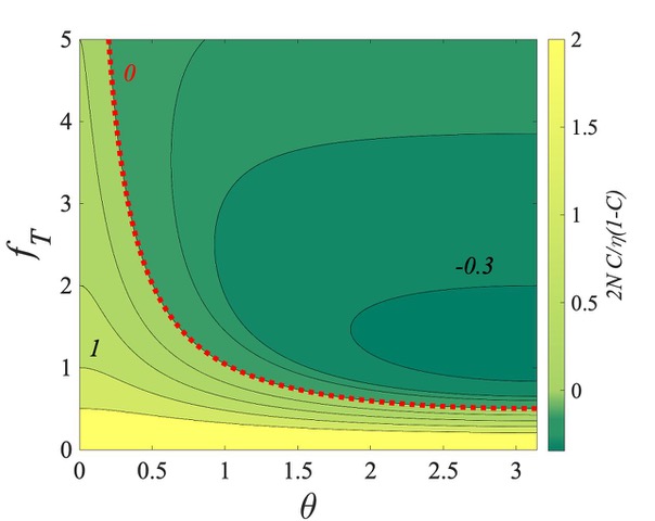
Figure 2: Plot of the renormalized contrast vs. the angle shift and the thermal noise

III.2 Perfectly correlated state

Correlated states involving qubits with equal $\nu$ but different $\mu$ improve the signal-to-noise ratio. More precisely, using the notation $\hat{S}_{\nu}^{i}=\sum_{\mu=1}^{M}\hat{\sigma}_{\nu,\mu}^{i}/2$, we notice from (III.1) that SNR for small $\Delta$ is proportional to $R=\langle\hat{S}_{\nu}^{x}\rangle/\langle\hat{S_{\nu}^{z}}^{2}\rangle^{1/2}$ which equals to $\sqrt{M}$ in the uncorrelated case. This observation suggests that the optimal state is the one that maximizes $R$ and therefore is the ground state of the quantum Ising Hamiltonian with a strong qubit-qubit coupling:

$$\hat{H}_{\nu}=\hat{S}_{\nu}^{z\,2}+\lambda\hat{S}_{\nu}^{x}$$ (24)

The coefficient $\lambda$ is the Lagrange multiplier that controls the necessary level of correlation. It should be small since an optimal result is obtained for strong quantum correlations. It is worth pointing out this connection between the magnetometry quantum sensing in cold atoms and the single photon detection using qubit detection. The optimization of SNR amounts to obtaining the highest possible spin squeezing Sørensen et al. (2001). Then we may use the perturbation theory. In the zeroth order ($\lambda\rightarrow 0$, we start from the total angular momentum state $|l,m\rangle_{\nu}$ as the eigenstate of ${\bf\hat{S}}^{2}_{\nu}=\sum_{i=x,y,z}\hat{S}_{\nu}^{i\,2}$ and $\hat{S}_{\nu}^{z}$ with eigenvalues $l(l+1)$ and $m$ respectively and where we identify $l=M/2$. The ground state combines states of $m$ very close to zero and thus corresponds to a giant spin state that entangles all the individual qubits.

In the next order, there are two cases:

$M$ odd: The next order is a linear combination of the two degenerate ground states $|M/2,\pm 1/2\rangle_{\nu}$. We find the correlated state $|\Psi\rangle=\prod_{\nu=1}^{N}(|M/2,1/2\rangle_{\nu}+|M/2,-1/2\rangle_{\nu})/\sqrt{2}$ that corresponds to a maximally entangled state. We determine that $\langle\delta^{2}\hat{S}^{z}_{\nu}\rangle=1/4$ is independent on $M$ and that $\langle\hat{S}^{x}_{\nu}\rangle=(M+1)/4$. We find therefore $R=(M+1)/2$ which corresponds asymptotically to the Heisenberg limit.

$M$ even: The ground state for $\lambda=0$ corresponds to a maximally entangled state of individual qubits:

$$|M/2,0\rangle_{\nu}=\frac{(M/2)!}{\sqrt{M!}}\!\!\!\!\!\!\sum_{\begin{array}[]{c}\tiny s_{\mu}=\pm 1/2\\ \tiny\!\!\!\!\!\!\!\sum_{\mu=1}^{M}s_{\mu}=0\end{array}}\!\!\!\!\!\!\!|s_{1},\dots,s_{\mu},\dots,s_{M}\rangle_{\nu}$$ (27)

with spin $s_{\mu}$ along the z axis. Each individual state is also an eigenstate for $\lambda=0$.

The expansion to the second order involves the entangled combination $|\Psi\rangle=\prod_{\nu=1}^{N}\sum_{m=-1}^{1}\alpha_{m}|M/2,m\rangle_{\nu}$. We determine $\langle\delta^{2}\hat{S}^{z}_{\nu}\rangle=\lambda^{2}(M/2+1)M/4$ and $\langle\hat{S}^{x}_{\nu}\rangle=\lambda(M/2+1)M/2$. We find therefore $R=\sqrt{M(M/2+1)}$ which also asymptotically tend to the Heisenberg limit which agrees with the results for squeezed spin states in André and Lukin (2002).

Such a maximally correlated state of the qubit set, which imposes the maximal rigidity on it producing a “giant spin”, is not realistic from the experimental point of view. Generally, restrictions imposed by the qubit circuit geometry limit their connectivity or couplings to architecture in clusters. A relaxation of effective qubit-qubit coupling affects the rigidity and deteriorate the SNR. Indeed, the introduction of a pertubation additional small term (which softens the ”giant spin”)

$$\hat{H}^{\prime}_{\nu}=\sum_{\mu\not=\mu^{\prime}=1}^{M}p_{\mu\mu^{\prime}}\frac{\hat{\sigma}^{z}_{\nu,\mu}\hat{\sigma}^{z}_{\nu,\mu^{\prime}}}{4}$$ (28)

raises the degeneracy of the individual states. Assume a simplified case where the interaction is turned on between $M-M_{E}$ spins and does not affect the $M_{E}$ other spins. For $M_{E}$ even, the state that minimizes the perturbation Hamiltonian for $\lambda=0$ can be decomposed into an uncorrelated state of $M-M_{E}$ spins and a perfectly correlated state of $M_{E}$ spins described by angular state with angular momentum number $M_{E}/2$ written as:

$$|\Psi\rangle_{\nu}=|\pm s_{1},\dots,\pm s_{M-M_{E}}\rangle|M_{E}/2,0\rangle_{\nu}$$ (29)

In this expression, there are two possible degenerate states of opposite uncorrelated spins. Again, as the result of second order perturbation theory, we obtain the expression for $R$,

$$R = \sqrt{M_{E}(M_{E}/2+1)+M-M_{E}}$$ (30)

which interpolates between the uncorrelated regime and the Heisenberg regime. Fig. 3 shows the increase of the SNR with the qubit number $M$ for various entanglement state characterized by the ratio $k=M_{E}/M$. This last result illustrates that the Heisenberg limit of SNR is not fragile with respect to perturbations.

$M=2$ for any $\lambda$: For this simpler situation, the exact diagonalization is possible. Using the correlated state $|\Psi\rangle=\prod_{\nu=1}^{N}\sum_{m=-1}^{1}\alpha_{m}|M/2,m\rangle_{\nu}$, we determine the coefficient $\alpha_{m}$ and find the ratio:

$$R=\sqrt{2+\frac{2}{\sqrt{1+4\lambda^{2}}}}$$ (31)

Thus $\lambda$ controls the crossover from an uncorrelated state ($R=\sqrt{2}$ at $\lambda=\infty$) to a fully correlated or entangled state ($R=2$ at $\lambda=0$), with the corresponding transition from the SQL to the Heisenberg limit.

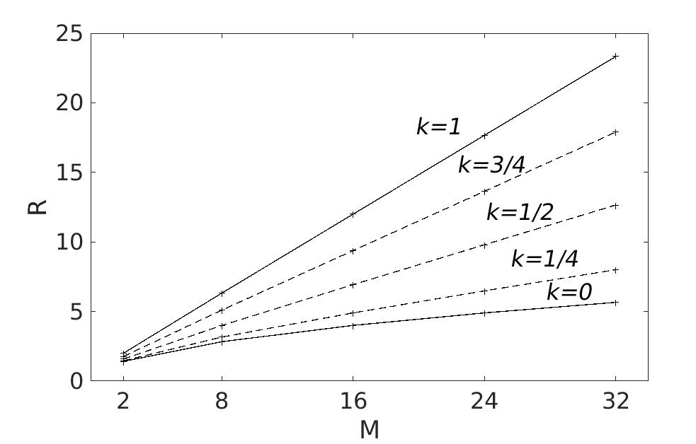
Figure 3: Signal to noise ratio $R$ vs. qubit number $M$ for perfect correlated state ($k=1$), non correlated state ($k=0$) and intermediate regimes ($0<k<1$)

III.3 Nearest-neighbour interacting state

Since the qubits are placed in a linear chain along the waveguide, we can use the quantum Ising Hamiltonian with only nearest-neighbour coupling:

$$\hat{H}_{\nu}=\sum_{\mu=1}^{M}\frac{\hat{\sigma}^{z}_{\nu,\mu+1}\hat{\sigma}^{z}_{\nu,\mu}}{2}+\lambda\frac{\hat{\sigma}^{x}_{\nu,\mu}}{2}$$ (32)

where we use periodic boundary condition for simplicity ($\hat{\sigma}^{z}_{\nu,M+1}=\hat{\sigma}^{z}_{\nu,1}$).

We define the antiferromagnetic state $|AF\rangle_{\nu}$ as the ground state for $\lambda=0$. These are two such degenerate states but we will only consider one since they are separated by a large potential barrier for large $N$. In the case of $\lambda\to 0$, we use again the second order perturbation theory with the correlated state $|\Psi\rangle=\prod_{\nu=1}^{N}(\alpha_{0}+\alpha_{1}\hat{S}^{+}_{\nu}+\alpha_{-1}\hat{S}^{-}_{\nu})|AF\rangle_{\nu}$. There are again two cases:

$M$ even: We find: $\langle\delta^{2}\hat{S}^{z}_{\nu}\rangle=\lambda^{2}M/16$ and $\langle\hat{S}^{x}_{\nu}\rangle=\lambda M/4$. Therefore we find no improvement since $R=\sqrt{M}$ is left unchanged.

$M$ odd: We find for large $M$ that $\langle\delta^{2}\hat{S}^{z}_{\nu}\rangle=(1+\lambda^{2}M/4)/4$ and $\langle\hat{S}^{x}_{\nu}\rangle=\lambda M/4$. We find therefore $R=\lambda M/\sqrt{4+\lambda^{2}M}\rightarrow\sqrt{M}$ for large $M$. In the limit of small $\lambda$ however, we find $R=\lambda M/2$ which is again the Heisenberg limit, but only achieved for $\lambda\langle\langle 1$.

Therefore the nearest-neighbour coupling is useless if the goal is to reach the Heisenberg limit of signal-to-noise ratio in a quantum detector array.

IV Conclusion

We have analyzed a detector consisting in an array of qubits in the presence of noise and interaction. Using an exactly solvable model, we have shown that quantum correlations of the state of array allow to reach the Heisenberg limit, that is, increase the signal-to-noise ratio proportionally to the total number of qubits (forming together the detected signal) rather than its square root. The rigidity of the qubit system is the crucial requirement for achieving this effect, which makes connectivity between qubits in a detector array the key parameter in designing similar systems. Our findings provide an important insight for strategy of reaching the Heisenberg limit, in the design of efficient qubit-based quantum detectors.

In our generic model we have neglected the size of the qubits compared to the microwave wavelength. We also do not specify the origin of the interaction, which produces the interqubit coupling. A natural extension of this study will be the investigation of different geometries of qubit arrays and of the effects of specifics of the interqubit interaction (dipole-dipole, inductive, etc.).

Acknowledgements: The authors thank K. Shulga for helpful discussions. This work was supported by the EU project SUPERGALAX (Grant agreement ID: 863313).

V Appendix

The expectation value of the phase is determined using the coherent state formalism. Defining the coherent state: $|\alpha\rangle_{\nu}=\sum_{n=0}^{\infty}e^{-|\alpha|^{2}/2}\alpha^{n}(\hat{a}^{\dagger}_{\nu})^{n}|0\rangle_{\nu,\mu}/n!$ and $|\beta\rangle_{\nu,\mu}=\sum_{n=0}^{\infty}e^{-|\beta|^{2}/2}\beta^{n}(\hat{b}^{\dagger}_{\nu,\mu})^{n}|0\rangle_{\nu,\mu}/n!$, we can calculate successively the coherent state average:

$${}_{\nu}\langle\alpha|_{\nu,\mu}\langle\beta|\exp[i\theta\hat{a}^{\prime\dagger}_{\nu,\mu}\hat{a}^{\prime}_{\nu,\mu}]|\alpha\rangle_{\nu}|\beta\rangle_{\nu,\mu} = {}_{\nu}\langle\alpha|_{\nu,\mu}\langle\beta|\exp[i\theta(\sqrt{\eta}\hat{a}^{\dagger}_{\nu}+\sqrt{1-\eta}\hat{b}^{\dagger}_{\nu,\mu})(\sqrt{\eta}\hat{a}_{\nu}+\sqrt{1-\eta}\hat{b}_{\nu,\mu})]|\alpha\rangle_{\nu}|\beta\rangle_{\nu,\mu}$$ (33)

$$= {}_{\nu}\langle 0|_{\nu,\mu}\langle 0|\exp[i\theta(\hat{a}^{\prime\dagger}_{\nu,\mu}+\sqrt{\eta}\alpha^{*}+\sqrt{1-\eta}\beta^{*})(\hat{a}^{\prime}_{\nu,\mu}+\sqrt{\eta}\alpha+\sqrt{1-\eta}\beta)]|0\rangle_{\nu}|0\rangle_{\nu,\mu}$$

$$= {}_{\nu,\mu}\langle\sqrt{\eta}\alpha+\sqrt{1-\eta}\beta|\exp[i\theta\hat{a}^{\prime\dagger}_{\nu,\mu}\hat{a}^{\prime}_{\nu,\mu}]|\sqrt{\eta}\alpha+\sqrt{1-\eta}\beta\rangle_{\nu,\mu}$$

$$= {}_{\nu,\mu}\langle\sqrt{\eta}\alpha+\sqrt{1-\eta}\beta|e^{i\theta}(\sqrt{\eta}\alpha+\sqrt{1-\eta}\beta)\rangle_{\nu,\mu}$$

$$= \exp[(e^{i\theta}-1)|\sqrt{\eta}\alpha+\sqrt{1-\eta}\beta|^{2}]$$

The thermal state caused by the noise is related to the coherent state through the formula:

$$\frac{\exp(-\hbar\omega_{k_{z}}\hat{b}^{\dagger}_{\nu,k_{z}}\hat{b}_{\nu,k_{z}}/k_{B}T)}{{\rm Tr}[\exp(-\hbar\omega_{k_{z}}\hat{b}^{\dagger}_{\nu,k_{z}}\hat{b}_{\nu,k_{z}}/k_{B}T)]}=\int\frac{d^{2}\beta}{\pi f_{k_{z}}}\exp(-|\beta|^{2}/f_{k_{z}})|\beta\rangle_{\nu,k_{z}}\langle\beta|$$ (34)

With this procedure, we obtain an expression for the thermal average:

$${\rm Tr}[|\alpha\rangle_{x}\langle\alpha|\frac{\exp(-\sum_{k_{z}=1}^{M}\hbar\omega_{k_{z}}\hat{b}^{\dagger}_{\nu,k_{z}}\hat{b}_{\nu,k_{z}}/k_{B}T)}{{\rm Tr}[\exp(-\sum_{k_{z}=1}^{M}\hbar\omega_{k_{z}}\hat{b}^{\dagger}_{\nu,k_{z}}\hat{b}_{\nu,k_{z}}/k_{B}T)]}\exp[i\theta\hat{a}^{\prime\dagger}_{\nu,\mu}\hat{a}^{\prime}_{\nu,\mu}]]$$ (35)

$$= \prod_{k_{z}=1}^{M}\int\frac{d^{2}\beta_{k_{z}}}{\pi f_{k_{z}}}\exp(-|\beta_{k_{z}}|^{2}/f_{k_{z}})\exp[(e^{i\theta}-1)|\sqrt{\eta}\alpha+\sqrt{1-\eta}\sum_{k_{z}=1}^{M}\frac{\exp(i2\pi k_{z}\nu/M)}{\sqrt{M}}\beta_{k_{z}}|^{2}]$$

$$= \frac{1}{1+f_{T}(1-e^{i\theta})}\exp\left[\frac{\eta(e^{i\theta}-1)|\alpha|^{2}}{1+f_{T}(1-e^{i\theta})}\right]$$

It remains to generalize the expressions for $N$ channels and carry out an expansion development in the photon number. Using the property that $|\alpha\rangle=\prod_{\nu=1}^{N}|\alpha/\sqrt{N}\rangle_{\nu}$, we determine

$$\langle\exp[i\theta a^{\prime\dagger}_{\nu,\mu}\hat{a}^{\prime}_{\nu,\mu}]\rangle = {\rm Tr}[|\alpha\rangle\langle\alpha|\frac{\exp(-\sum_{\nu^{\prime},k_{z}=1}^{N,M}\hbar\omega_{k_{z}}\hat{b}^{\dagger}_{\nu^{\prime},k_{z}}\hat{b}_{\nu^{\prime},k_{z}}/k_{B}T)}{{\rm Tr}[\exp(-\sum_{\nu^{\prime},k_{z}=1}^{N,M}\hbar\omega_{k_{z}}\hat{b}^{\dagger}_{\nu^{\prime},k_{z}}\hat{b}_{\nu^{\prime},k_{z}}/k_{B}T)]}\exp[i\theta a^{\prime\dagger}_{\nu,\mu}\hat{a}^{\prime}_{\nu,\mu}]$$ (36)

$$= \frac{1}{1+f_{T}(1-e^{i\theta})}\exp\left[\frac{\eta(e^{i\theta}-1)|\alpha|^{2}}{N[1+f_{T}(1-e^{i\theta})}\right]$$

Finally, by an expansion in $\alpha$, we deduce the average for the case of $n$ photons:

$$\langle\exp[i\theta a^{\prime\dagger}_{\nu,\mu}\hat{a}^{\prime}_{\nu,\mu}]\rangle_{n} = {\rm Tr}[|n\rangle\langle n|\frac{\exp(-\sum_{\nu^{\prime},k_{z}=1}^{N,M}\hbar\omega_{k_{z}}\hat{b}^{\dagger}_{\nu^{\prime},k_{z}}\hat{b}_{\nu^{\prime},k_{z}}/k_{B}T)}{{\rm Tr}[\exp(-\sum_{\nu^{\prime},k_{z}=1}^{N,M}\hbar\omega_{k_{z}}\hat{b}^{\dagger}_{\nu^{\prime},k_{z}}\hat{b}_{\nu^{\prime},k_{z}}/k_{B}T)]}\exp[i\theta a^{\prime\dagger}_{\nu,\mu}\hat{a}^{\prime}_{\nu,\mu}]$$ (37)

$$= \frac{1}{1+f_{T}(1-e^{i\theta})}\left[1+\frac{\eta(e^{i\theta}-1)}{N[1+f_{T}(1-e^{i\theta})}\right]^{n}$$

References

• Ren et al. (2017) J.-G. Ren, P. Xu, H.-L. Yong, L. Zhang, S.-K. Liao, J. Yin, W.-Y. Liu, W.-Q. Cai, M. Yang, L. Li, et al., Nature 549, 70 (2017).
• Santagati et al. (2019) R. Santagati, A. A. Gentile, S. Knauer, S. Schmitt, S. Paesani, C. Granade, N. Wiebe, C. Osterkamp, L. P. McGuinness, J. Wang, M. G. Thompson, J. G. Rarity, F. Jelezko,  and A. Laing, Phys. Rev. X 9, 021019 (2019).
• Kiani et al. (2020) B. T. Kiani, A. Villanyi,  and S. Lloyd, “Quantum medical imaging algorithms,”  (2020), arXiv:2004.02036 [quant-ph] .
• Duffy and van Bibber (2009) L. D. Duffy and K. van Bibber, New Journal of Physics 11, 105008 (2009).
• Beck (2015) C. Beck, Physics of the Dark Universe 7-8, 6 (2015).
• Dixit et al. (2020) A. V. Dixit, S. Chakram, K. He, A. Agrawal, R. K. Naik, D. I. Schuster,  and A. Chou, “Searching for dark matter with a superconducting qubit,”  (2020), arXiv:2008.12231 [hep-ex] .
• Zagoskin (2011) A. M. Zagoskin, Quantum engineering: theory and design of quantum coherent structures (Cambridge University Press, 2011).
• Schuster et al. (2007) D. I. Schuster, A. A. Houck, J. A. Schreier, A. Wallraff, J. M. Gambetta, A. Blais, L. Frunzio, J. Majer, B. Johnson, M. H. Devoret, S. M. Girvin,  and R. J. Schoelkopf, Nature 445, 515 (2007).
• Inomata et al. (2016) K. Inomata, Z. Lin, K. Koshino, W. D. Oliver, J.-S. Tsai, T. Yamamoto,  and Y. Nakamura, Nature Communications 7, 12303 (2016).
• Gu et al. (2017) X. Gu, A. F. Kockum, A. Miranowicz, Y. xi Liu,  and F. Nori, Physics Reports 718-719, 1 (2017), microwave photonics with superconducting quantum circuits.
• Sathyamoorthy et al. (2014) S. R. Sathyamoorthy, L. Tornberg, A. F. Kockum, B. Q. Baragiola, J. Combes, C. M. Wilson, T. M. Stace,  and G. Johansson, Phys. Rev. Lett. 112, 093601 (2014).
• Paik et al. (2011) H. Paik, D. I. Schuster, L. S. Bishop, G. Kirchmair, G. Catelani, A. P. Sears, B. R. Johnson, M. J. Reagor, L. Frunzio, L. I. Glazman, S. M. Girvin, M. H. Devoret,  and R. J. Schoelkopf, Phys. Rev. Lett. 107, 240501 (2011).
• Koch et al. (2007) J. Koch, T. M. Yu, J. Gambetta, A. A. Houck, D. I. Schuster, J. Majer, A. Blais, M. H. Devoret, S. M. Girvin,  and R. J. Schoelkopf, Phys. Rev. A 76, 042319 (2007).
• Wendin (2017) G. Wendin, Reports on Progress in Physics 80, 106001 (2017).
• Wallraff et al. (2004) A. Wallraff, D. I. Schuster, A. Blais, L. Frunzio, R.-S. Huang, J. Majer, S. Kumar, S. M. Girvin,  and R. J. Schoelkopf, Nature 431, 162 (2004).
• Il’ichev et al. (2003) E. Il’ichev, N. Oukhanski, A. Izmalkov, T. Wagner, M. Grajcar, H.-G. Meyer, A. Y. Smirnov, A. Maassen van den Brink, M. H. S. Amin,  and A. M. Zagoskin, Phys. Rev. Lett. 91, 097906 (2003).
• Hoi et al. (2013) I.-C. Hoi, C. M. Wilson, G. Johansson, J. Lindkvist, B. Peropadre, T. Palomaki,  and P. Delsing, New Journal of Physics 15, 025011 (2013).
• Rakhmanov et al. (2008) A. L. Rakhmanov, A. M. Zagoskin, S. Savel’ev,  and F. Nori, Physical Review B 77, 144507 (2008).
• Zagoskin et al. (2009) A. Zagoskin, A. Rakhmanov, S. Savel’ev,  and F. Nori, physica status solidi (b) 246, 955 (2009).
• Savel’ev et al. (2012) S. Savel’ev, A. Zagoskin, A. Rakhmanov, A. Omelyanchouk, Z. Washington,  and F. Nori, Physical Review A 85, 013811 (2012).
• Ivić et al. (2016) Z. Ivić, N. Lazarides,  and G. Tsironis, Scientific reports 6, 29374 (2016).
• Grimsmo et al. (2020) A. L. Grimsmo, B. Royer, J. M. Kreikebaum, Y. Ye, K. O’Brien, I. Siddiqi,  and A. Blais, “Quantum metamaterial for nondestructive microwave photon counting,”  (2020), arXiv:2005.06483 [quant-ph] .
• Zagoskin et al. (2013) A. M. Zagoskin, R. D. Wilson, M. Everitt, S. Savel’ev, D. R. Gulevich, J. Allen, V. K. Dubrovich,  and E. Il’ichev, Scientific Reports 3 (2013), 10.1038/srep03464.
• Giovannetti et al. (2006) V. Giovannetti, S. Lloyd,  and L. Maccone, Phys. Rev. Lett. 96, 010401 (2006).
• Giovannetti et al. (2004) V. Giovannetti, S. Lloyd,  and L. Maccone, Science 306, 1330 (2004).
• Shlyakhov et al. (2018) A. R. Shlyakhov, V. V. Zemlyanov, M. V. Suslov, A. V. Lebedev, G. S. Paraoanu, G. B. Lesovik,  and G. Blatter, Phys. Rev. A 97, 022115 (2018).
• Danilin et al. (2018) S. Danilin, A. V. Lebedev, A. Vepsäläinen, G. B. Lesovik, G. Blatter,  and G. S. Paraoanu, npj Quantum Information 4 (2018), 10.1038/s41534-018-0078-y.
• Sørensen et al. (2001) A. Sørensen, L.-M. Duan, J. I. Cirac,  and P. Zoller, Nature 409, 63 (2001).
• André and Lukin (2002) A. André and M. D. Lukin, Phys. Rev. A 65, 053819 (2002).