Augmented Convolutional LSTMs for Generation of High-Resolution Climate Change Projections

Abstract.

Projection of changes in extreme indices of climate variables such as temperature and precipitation are critical to assess the potential impacts of climate change on human-made and natural systems, including critical infrastructures and ecosystems. While impact assessment and adaptation planning rely on high-resolution projections (typically in the order of a few kilometers), state-of-the-art Earth System Models (ESMs) are available at spatial resolutions of few hundreds of kilometers. Current solutions to obtain high-resolution projections of ESMs include downscaling approaches that consider the information at a coarse-scale to make predictions at local scales. Complex and non-linear interdependence among local climate variables (e.g., temperature and precipitation) and large-scale predictors (e.g., pressure fields) motivate the use of neural network-based super-resolution architectures. In this work, we present auxiliary variables informed spatio-temporal neural architecture for statistical downscaling. The current study performs daily downscaling of precipitation variable from an ESM output at 1.15 degrees ( 115 km) to 0.25 degrees (25 km) over the world’s most climatically diversified country, India. We showcase significant improvement gain against three popular state-of-the-art baselines with a better ability to predict extreme events. To facilitate reproducible research, we make available all the codes, processed datasets, and trained models in the public domain.

1. Introduction

The last few decades have witnessed record-breaking climate and weather-related extremes across the globe (Prein et al., 2017; Zhang et al., 2013). We are witnessing urgent calls for substantial new investments in climate modeling to increase the precision, accuracy, reliability, and resolution at which information is made available to the stakeholders (Dessai et al., 2009b; Schmidt, 2010). To model earth’s past, present, and future climate, Earth System Models are used for simulate the interactions of atmosphere, land, ocean, ice and biosphere to estimate the state of local and regional climate under various conditions. Earth system models (ESMs) integrate the interactions of atmosphere, ocean, land, ice, and biosphere to estimate the state of regional and global climate under a wide variety of conditions (Arora et al., 2013). Despite the increasing complexity and inclusion of more sophisticated schemes to account for interactions across various constituting components, ESMs suffer from three broad sources of uncertainties: (i) knowledge gaps in understanding of coupled natural-human systems which could results in different Representative Concentration Pathways (RCPs), (ii) lack of understanding of physics of climate system which is encapsulated through parametric differences in Multiple Model Ensembles (MMEs), and (iii) intrinsic variability which is captured through multiple initial condition ensembles (Kumar and Ganguly, 2018). To characterize these uncertainties, ESMs are often executed with multiple initial conditions, multiple ensemble mode with different RCPs making impact relevant insight discovery from ESM outputs a “big data” challenge (Faghmous and Kumar, 2014). Owing to ESMs high-computation requirements, their projections are limited to a very coarse resolution (typically 100–150 km), leading to complications in assessing the regional impacts (Wilby and Dessai, 2010; Dessai et al., 2009a). While there has been an emphasis on multiple model ensembles for assessing climate change impacts on precipitation and temperature, researchers believe that ignoring the contribution of internal variability could result in underestimation of statistics of extremes, which in turn can lead to maladaptation (Bhatia and Ganguly, 2019). However, the development of design relevant intensity-duration and frequency curves require climate projections at high resolution. Hence, generating high-resolution data products that have high credibility is pivotal to inform adaptation strategies in the backdrop of climate change.

1.1. The Downscaling Approaches

Climate scientists use downscaling techniques to generate climate projections at higher spatial resolution. These techniques are broadly classified into two categories, namely dynamical and statisti‘cal downscaling. Dynamical downscaling embeds the sub-grid processes within boundary conditions of coarse resolution ESM grids. Examples of sub-grid processes include cloud physics, radiation, soil characteristics, and hydrological processes. While dynamical downscaling is useful for simulating extreme precipitation events and localized phenomena such as convective precipitations, the generated outputs are highly sensitive to the boundary conditions (Xue et al., 2014). High computational requirements and limited spatial scalability limit the usage in downscaling multiple ensembles, and multiple initial conditions runs of ESMs. On the other hand, statistical downscaling (hereafter ‘SD’) attempts to learn the statistical relationship between ESM output (at coarse resolution) with high-resolution observations such as observed or remotely sensed precipitation. With an underlying assumption of space and time stationarity, the above relationship helps in generating higher resolution outputs of coarse resolution ESM projections.

1.2. Climatically Diversified Indian Sub-continent

Indian subcontinent comprises a wide range of weather conditions and six climate subtypes ranging from tundra and glaciers in the north to deserts in the west, and humid tropical regions in the southwest. Indian subcontinent comprises of wide range and highly disparate micro-climate systems, making it one of the most climatically diverse countries on the globe (Brenkert and Malone, 2005). Despite the stark heterogeneity, these geographical and geological features work in tandem to drive Indian Summer Monsoon Rainfall (or ISMR) (Kulkarni et al., 2009; Clift and Plumb, 2008). India receives 80% of its annual rainfall during the southwest summer monsoon season. While monsoon systems are reliable at annual scales as a consequence of seasonal heating of the land, even small percentage variations (Mishra et al., 2012) can have dramatic impacts on food and economic security of the nation (Gadgil and Gadgil, 2006). In addition to regional and local correlations in space and time, ISMR is influenced by the coupled ocean and atmospheric phenomena over the Indian Ocean, Pacific decadal oscillations, and Atlantic Ocean sea surface temperature making it a complicated system to predict. Given the utmost importance of ISMR in the Indian Climatic system, we have trained the proposed model separately for monsoon and non-monsoon seasons in the context of SD.

1.3. Spatio-temporal Teleconnections

In atmospheric sciences, climate variables and anomalies often exhibit long-term dependence among spatially non-contiguous regions, referred to as “teleconnections” (Adarsh and Reddy, 2019). Analogously, it is widely accepted that climate variability is scale-invariant and exhibit long-term memory in time (Yuan et al., 2013). Here, long-term memory implies that the present state of the system influences the future states. Recent advancements in deep learning literature result in several SD architectures such as Convolution Neural Networks (CNNs) (Vandal et al., 2017), Residual Dense Block (RDB) (Zhang et al., 2018) and Long Short Term Memory (LSTMs) (Misra et al., 2018) capturing spatial and temporal dependencies, respectively.

However, to the best of our knowledge, we do not find any SD technique that captures both spatio-temporal dependencies simultaneously. Moreover, we showcase that both CNN-based approaches (Vandal et al., 2017) and RDB based approaches that generates high-resolution projections of ESM using a single image does not perform well when applied to real ESM data.

1.4. Augmented Convolutional LSTMs

In this paper, we address the major limitation of SD techniques in capturing spatio-temporal dependencies simultaneously. We discuss a framework to downscale multiple initial condition ensembles of Community Earth System Model Large Ensemble (CESM-LENS) project (Kay et al., 2015) using Recurrent Convolutional LSTM. Besides, we propose a research direction to augment multiple state variables in addition to station elevation data by including seven physics guided auxiliary variables.

1.5. Key Contributions

The key contributions are as follows:

• We present a Recurrent Convolutional LSTM based Super-resolution approach towards statistical downscaling of climatic data from coarse-resolution ESM to fine-resolution Observation data, which accounts for spatial and temporal dependence in space and time between target variable (precipitation in the present case) and auxiliary variables. We propose a way to include multiple state variables in addition to station elevation data by including seven physics guided auxiliary variables.

• We address the major limitation of state-of-the-art deep learning-based super-resolution architectures that use a coarse resolution version of the same image to generate finer resolution outputs. Moreover, in reality, ESMs are expected to capture statistics of atmospheric variables, especially at decadal and interdecadal scales. Hence, day-to-day mapping, as proposed by earlier models, is of limited to no use to multiple downscale models and multiple ensembles of ESMs.

1.6. Organization of the Paper:

We organize the rest of the paper as follows. Section 2 outlines data used in present research along with the rationale of choice of covariates. Section 3 discusses the related work in the area of SD along with an overview of state-of-the-art convolution neural network and LSTM based approaches for SD and their key limitations. Section 4 presents ConvLSTM for SD. Section 5 describes the experimental settings. In Section 6, we compare our results with the current state-of-the-art ResLap (Cheng et al., 2020), DeepSD (Vandal et al., 2017) and widely used quantile mapping technique (Cannon, 2011). In Section 7, we briefly discuss results, limitations, and scalability potential of our work to generate high-resolution outputs that can be leveraged by stakeholders and policymakers for design and adaptation planning.

2. Datasets

Climate modeling relies on the numerical solution of the fundamental equations for atmospheric motion, i.e., conservation of mass, energy, and momentum, and equation of state, which are expressed as simultaneous non-linear dynamical equations (Hansen et al., 1983). The solution of these equations typically yields state variables including temperature, humidity, atmospheric pressure, wind velocities in three directions (zonal, meridional, and vertical velocities), and precipitation. However, running the climate models or ESMs at higher temporal resolutions results in higher computation cost since the relationship between spatial resolution and model execution time is non-linear; hence these models run at the resolution of a 100–150 km resulting in too coarse resolution for local and regional adaptation. In this paper, we use coarse resolution precipitation outputs from the NCAR Community Earth System Model (NCAR CESM1 CAM5) obtained from the archives of the Climate Modeling Intercomparison Project 5 (Lauritzen et al., 2018; Taylor et al., 2012). To establish the relationship between coarse resolution model output and observations at high resolution, we use the high-resolution spatial resolution ($0.25^{o}\times 0.25^{o})$ available for 110 years over the Indian mainland (Pai et al., 2014). As precipitation is also dependent upon temperature, humidity, atmospheric pressure, and wind velocities, we use these variables as potential covariates in addition to coarse resolution precipitation. Since observations for these covariates is not available at the gauge level, we use the outputs from the national Centers for Environmental Prediction-National Center for Atmospheric Research (NCEP-NCAR) global reanalysis project (Kalnay et al., 1996). Furthermore, the correlation between precipitation patterns and topography suggests that type (rain or snow), intensity, and duration of precipitation is significantly controlled by elevation characteristics. Hence, we use the topographical information from NASA’s Shuttle Radar Topography Mission (SRTM), which is available at 90 meters. As outlined in (Vandal et al., 2017), we use the image construct to combine coarse resolution precipitation with covariates and elevation data (jointly referred to as ‘auxiliary variables’), resulting in a 7-channel input image. One advantage of retaining image-based construct over other machine learning-based approaches of SD is that it preserves the spatial dependence structure. Section 5.1 presents detailed description of datasets with experimental settings.

Figure 1. (Best viewed in color) An example of temporal dependence of precipitation over a span of three days. Red color represents regions of high precipitation, whereas Blue color represents regions with low precipitation.

3. Related Work

As discussed before, SD is a technique for obtaining high-resolution climate and/or climate change information at adaptation relevant scales. SD has been applied to coarse resolution ESM output for years with a rich body of work existing in this field. SD is typically viewed as a problem of regression with the objective of identifying the optimal transfer function between ESM inputs and observations. Both linear and non-linear approaches are used to establish the relationship between auxiliary variables and the target variable of interest. Popular approaches among others include linear regression methods (Wilby and Wigley, 1997), Automated Statistical Downscaling (ASD) (Guo et al., 2012), relevance vector machines (Ghosh and Mujumdar, 2008), zero-shot super-resolution architecture (Shocher et al., 2018), quantile regression neural network (Cannon, 2011), and multivariate linear regression approach (Chen et al., 2010). Another widely used approach is quantile mapping methods (Cannon et al., 2015), which correct systematic biases in the distribution of climate variables. While these approaches are sufficient to capture mean statistics of climate variables, it has been found that these approaches fail in capturing extremes. Moreover, while quantile mapping methods have gained wider popularity, these tend to corrupt the trends projected by models artificially (Cannon et al., 2015).

Given the spatiotemporal nature and underlying non-linear behavior of the climate system, there is growing interest in the adaptation of deep learning techniques based super-resolution architectures to statistical downscaling. Vandal et al. (Thomas Vandal, 2017) proposed DeepSD which considered the complex precipitation data as a single image. DeepSD (Thomas Vandal, 2017) consists of convolution neural networks based super-resolution architecture SRCNN (Dong et al., 2014a) to capture the spatial dependencies. Inspired by this, other researchers have proposed ResLap (Cheng et al., 2020) which uses laplacian pyramid based super-resolution network (Lai et al., 2017) for further improvement in the quality of the generated climate change projections. ResLap (Cheng et al., 2020) extracts hierarchical features from the original precipitation projection and used a series of transposed convolution networks to upscale the low-resolution projection to the target scale. On other hand, given the long short term memory processes that are inherent to the system, researchers have also used recurrent and vanilla Long Short Term Memory (LSTM) (Misra et al., 2017) for climate downscaling. Moreover, in the context of SD using super-resolution construct, authors have envisioned the problem of SD as that of a single image Super-resolution. However, this approach has two major limitations. First, ESMs are designed to capture the statistics of climate variables, and there is no concept of one-to-one mapping with observations. Hence, single image Super-resolution can yield superfluous results when applied to real ESMs. Secondly, while both DeepSD(Thomas Vandal, 2017) and ResLap(Cheng et al., 2020) accounts for dependencies in space, temporal dependencies are altogether ignored, which are ubiquitous in climate and weather patterns, as shown in Fig 1. To capture temporal dependence, (Misra et al., 2017) used Long-Short Term Memory (LSTM) recurrent neural network. LSTMS are commonly used for processing sequential inputs and are preferred over vanilla RNNs as they solve the problem of vanishing gradients to some extent. However, one of the essential requirements for LSTMs is that it requires a one-dimensional data stream. So, in order to fit this with the problem, authors flattened the image to form a single-dimensional array and passed it to LSTMs, resulting in loss of spatial structure. To our knowledge, little work has been attempted to explicitly capture dependency in space and time in the context of SD.

4. Methodology

In this section, we present a detailed discussion of our proposed SD methodology. The proposed deep architecture addresses the problems described in the previous section.

4.1. Convolutional LSTM Networks for SD

We envision the problem of SD as learning the transfer function between high-resolution observations and coarse resolution ESM outputs using a spatio-temporal sequence of state variables as input. By combining fully connected LSTMs with convolutions, we build an end-to-end trainable convolutional LSTM SR (ConvLSTM-SR) model for SD problem that combines convolutional LSTMs (Xingjian et al., 2015) with super-resolution block (discussed next).

4.2. Model Description

Consider $X_{t}$ representing low resolution spatial data at $t^{th}$ day consisting of seven channels, each representing one climate variable. Each $X_{t}$ represents an “image” of size 7$\times$N$\times$M, where last two dimensions representing spatial dimensions. Consider $\mathcal{X}_{t}$ representing previous $T$ low resolution spatial data points available on $t^{th}$ day:

(1) $$\mathcal{X}_{t}=[X_{t-T},X_{t-(T-1)},X_{t-(T-2)},\ldots,X_{t-1},X_{t}]$$

We define convolutional LSTM, $ConvLSTM(\eta,k)$, where $\eta$ and $k$ represent number of filters and kernel dimensions, respectively. Convolutional LSTM handles spatio-temporal data by considering cell outputs $C_{1},\ldots,C_{t}$, hidden states $H_{1},\ldots,H_{t}$, and gates, $i_{t}$ (input), $f_{t}$(forget) and $o_{t}$ (output) as 3D tensors. The equation below (Shi et al., 2015) illustrates operations at different gates with $\ast$ and $\circ$ representing convolution and element-wise matrix multiplication operations, respectively.

(2) $$i_{t}=Sigmoid(W_{i}\ast\mathcal{X}_{t}+R_{i}\ast h_{t-1}+\rho_{i}\circ C_{t-1}+b_{i})$$

(3) $$f_{t}=Sigmoid(W_{f}\ast\mathcal{X}_{t}+R_{f}\ast h_{t-1}+\rho_{f}\circ C_{t-1}+b_{f})$$

(4) $$o_{t}=Sigmoid(W_{o}\ast\mathcal{X}_{t}+R_{o}\ast h_{t-1}+\rho_{o}\circ C_{t}+b_{o})$$

(5) $$C_{t}=f_{t}\circ c_{t-1}+i_{t}\circ Tanh(W_{c}\mathcal{X}_{t}+R_{c}h_{t-1}+b_{c})$$

(6) $$h_{t}=o_{t}\circ Tanh(c_{t})$$

In the above equations, $W_{i}$, $W_{f}$, $W_{o}$ and $W_{c}$ $\in$ $\mathbb{R}^{\eta,k,k}$ represent input weights, $R_{i}$, $R_{f}$, $R_{o}$ and $R_{c}$ $\in$ $\mathbb{R}^{\eta,k,k}$ represent recurrent weights, $\rho_{i}$, $\rho_{f}$, and $\rho_{o}$ $\in$ $\mathbb{R}^{k}$ represent peephole weights and $b_{i}$, $b_{f}$, $b_{o}$ and $b_{c}$ $\in$ $\mathbb{R}^{k}$ represent bias weights. Fig 2 shows the detailed description of ConvLSTM block.

Figure 2. (a) A detailed Representation of ConvLSTM block. (b) Representation of Super-resolution (SR) block. The labels of each block follows the convention of name of the layer followed by its activation and an integer represents the number of kernels used in that particular block.

We propose a stacked ConvLSTM architecture, comprising three stacked ConvLSTM blocks and a super-resolution (SR) block. The first ConvLSTM block attempts to encode the temporal information present in the sequence while maintaining the spatial dependencies between them with total $\eta_{1}$ filters of $k_{1}\times k_{1}$ dimensions.

(7) $$F_{1}(\mathcal{X})=ConvLSTM(\eta_{1},k_{1})(\mathcal{X})$$

Similarly, second ConvLSTM block comprises $\eta_{2}$ filters each with $k_{2}\times k_{2}$ dimensions.

(8) $$F_{2}(\mathcal{X})=ConvLSTM(\eta_{2},k_{2})(F_{1}(\mathcal{X}))$$

The last ConvLSTM block comprises $\eta_{3}$ filters each with $k_{3}\times k_{3}$ dimensions.

(9) $$F_{3}(\mathcal{X})=ConvLSTM(\eta_{3},k_{3})(F_{2}(\mathcal{X}))$$

In our experiments, we choose $N$ and $M$ as 129 and 135. We choose $\eta_{1}$, $\eta_{2}$, $\eta_{3}$ as 32, 16, and 16, respectively. Similarly, we choose $k_{1}$, $k_{2}$, and $k_{3}$ as 9, 5, 3, respectively. The size of the resultant output tensor after three stacked ConvLSTM operations is 16$\times$129$\times$135. The recurrent nature associated with the ConvLSTM helps in utilizing the temporal dependencies associated with data. On the other hand, the convolutional operations inside the cell help in retaining the spatial correlation. Therefore, The output tensor encodes temporal as well as the spatial dependencies associated with the data.

The super-resolution (SR) block (described in Fig 2) increases the resolution of high dimensional feature data obtained from the preceding ConvLSTM layers. In our experiments, SR block consist of a six stacked deep Convolutional layers with skip connections in between them. Each convolution layer has Relu activation (Nair and Hinton, 2010). Below shows operation sequence inside the Super-resolution (SR) block. $W^{\prime}_{1}$, $W^{\prime}_{2}$, ,$W^{\prime}_{3}$ and $W^{\prime}_{4}$ represent filters of size 16$\times$9$\times$9, 128$\times$5$\times$5 and 64$\times$3$\times$3, 32$\times$3$\times$3 respectively. $B^{\prime}_{1}$, $B^{\prime}_{2}$, and $B^{\prime}_{3}$ represent bias weights.

(10) $$F^{\prime}_{1}(X)=W^{\prime}_{1}\ast X+B^{\prime}_{1}\\$$

(11) $$F^{\prime}_{2}(X)=ReLU(W^{\prime}_{2}\ast F^{\prime}_{1}(X)+B^{\prime}_{2})\\$$

(12) $$F^{\prime}_{3}(X)=ReLU(W^{\prime}_{3}\ast F^{\prime}_{2}(X)+B^{\prime}_{3})\\$$

(13) $$F^{\prime}_{4}(X)=CONCAT(F^{\prime}_{1}(X),F^{\prime}_{3}(X))\\$$

(14) $$F^{\prime}_{5}(X)=W^{\prime}_{4}\ast X+B^{\prime}_{4}$$

As described above, the high-resolution feature data processed produced from the last ConvLSTM layer is passed to the first SR block.

(15) $$F_{4}(\mathcal{X})=SRBlock(F_{3}(\mathcal{X}))$$

The output from the first SR block is further passed through another SR block for doubling the current resolution.

(16) $$F_{5}(\mathcal{X})=SRBlock(F_{4}(\mathcal{X}))$$

(17) $$F_{6}(\mathcal{X})=ReLU(W^{\prime\prime}_{1}\ast F_{5}(\mathcal{X})+B^{\prime\prime}_{1})$$

(18) $$F_{7}(\mathcal{X})=W^{\prime\prime}_{2}\ast F_{6}(\mathcal{X})+B^{\prime\prime}_{2}$$

In our experiments  (17) and  (18), $W^{\prime\prime}_{1}$ and $W^{\prime\prime}_{2}$ represent filters of size 128$\times$1$\times$1 and 16$\times$3$\times$3, respectively. $B^{\prime\prime}_{1}$ and $B^{\prime\prime}_{2}$ represent bias weights. The overall architecture is shown in Fig 3.

Figure 3. Proposed Convolutional LSTM based model augmented with Super-resolution block. On left, the representation of all the 7 climatic variables (Precipitation, Elevation, Relative-Humidity, Pressure, 3 Wind components) as channels is shown. The numbers mentioned in the labels of each block followed by its name and activation represents the number of kernels used in that particular block.

5. Experiments

This section describes the dataset and the experimental settings.

5.1. Dataset

Owing to the diversity in the Indian precipitation profile, we categorize months into two periods: (i) Non-monsoon (October – April) and (ii) Monsoon months (May – September). Since the spatial resolution of the ESM(1.15°), the reanalysis state variables(2°) and observations(0.25°) are different, therefore, we interpolate both the ESM and the reanalysis state variables to match the resolution of the observation. We train our proposed model for these periods separately. In addition, each variable is normalized for better representation. Except for precipitation, all climate variables are normalized between 0 and 1. Precipitation is normalized between 0 and 50. This differential normalization scheme explicitly focuses the model on the precipitation variable compared to other auxiliary variables.

Table 1. Dataset statistics

Overall	Year-range	1948–2005
	Climate variables	7
	Total instances	21,170
	Input shape (interpolated)	$7\times 129\times 135$
	Output Shape	$1\times 129\times 135$
Test	Year-range	2000–2005
	Instances	2,190
Train	Year-range	1948–1999
	Instances	20,075

We, further, split data into train and test classes. The training data comprises years between 1948–1999, whereas test data comprises years between 2000–2005.

5.2. Experimental settings

5.2.1. Parameter Training

The proposed model generates fine-grained precipitation projections leveraging previous five days coarse-grained climatic projections. We incorporate recurrent dropouts of $0.2$ to the stacked ConvLSTM layers along with a dropout of $0.1$ between ConvLSTM layers. Additionally, we keep regularization with weight decay of value $0.02$ in the ConvLSTM layers. The RMSE loss is optimized using Adam optimizer (Kingma and Ba, 2014). Besides, we keep an adaptive learning rate ($lr$) with an initial value of $0.0003$. The subsequent rates follow the update equation, $lr=lr*\alpha$, where $\alpha=0.2$. The models for both monsoon and non-monsoon periods have an identical set of parameters. Both the models are trained for 1500 epochs with the mini-batch size as 15. Models were built and trained on Tensorflow (Abadi et al., 2016). For training, two NVIDIA RTX 2080-Ti GPUs were harnessed by independently training the two models (monsoon and non-monsoon) on each of them.

5.3. Baselines

We compare our proposed model with two state-of-the-art baselines, ResLap (Zhang et al., 2018; Cheng et al., 2020), DeepSD (Vandal et al., 2017) and Quantile Mapping Approach (Cannon et al., 2015).

5.3.1. ResLap(Cheng et al., 2020)

It uses a Residual Dense Block (RDB) on top of Laplacian pyramid based super-resolution network (Lai et al., 2017) for generating high resolution climate change projections. ResLap (Cheng et al., 2020) extracts hierarchical features at different levels from the original precipitation projection. It then uses a series of transposed convolution networks to upscale the low-resolution projection to the target scale.

5.3.2. DeepSD (Vandal et al., 2017)

It uses a series of stacked convolutional neural network-based super-resolution architecture SRCNN (Dong et al., 2014a). Each of the stacked SRCNN (Dong et al., 2014a) module in DeepSD (Thomas Vandal, 2017) is trained independently to generate climate change projection at different resolutions. Low-resolution projection is then passed sequentially through this stacked pipeline to finally generate the high resolution climate projections.

5.3.3. Quantile Mapping Approach (Q-Map) (Cannon et al., 2015)

Bias Correction Spatial Disaggregation (BCSD) or Quantile mapping approach follows a point based statistical estimation. It is a simple but effective method for statistical downscaling. These models correct systematic biases in distribution of climate variables.

5.4. Evaluation Metrics

We leverage root-mean-square error (RMSE), and mean of absolute difference (referred to as Bias) to compare our proposed model with the state-of-the-art frameworks for statistical downscaling of climate variables ResLap, DeepSD and popularly used Q-Map.

5.5. Choice of lag-days

While in present studies, we have five temporal inputs with a lag of four, we note that the inclusion of a higher number of temporal variables could result in better performance. However, in this case, our choice of lag is limited by the computing power at our disposal. For this study, we used Nvidia-RTX-2080Ti with a batch size of 15.

5.6. Comparison

In this work, we compare the performance of the proposed approach with state-of-the-art methods, including ResLap, DeepSD and Quantile mapping. DeepSD, a convolutional neural network-based super-resolution approach for SD (Thomas Vandal, 2017), recently gained popularity, given its accuracy on a single image super-resolution task. On the other hand, Q-Map (Cannon, 2011) is a simple yet elegant technique that is widely used for the SD problem.

In our experiments, we apply quantile mapping on daily precipitation to match the probability distribution function of ESM outputs with observations by inverting the cumulative distribution functions. This inversion leads to the removal of systematic bias. Since the spatial resolution of ESM and observations is different, we interpolate ESM to common grid resolution to match the observation grid. We note that while the grid size is reduced, mere interpolation does not account for increased resolution as fine-scale information is missing from the interpolated image. The process of interpolation is followed by determining the scaling factors to map the distribution of interpolated ESM outputs to observations. The projections for the year 2000–2005 are used for comparison to BCSD.

Secondly, ResLap is applied to downscale over India using coarse resolutions from ESM and it’s corresponding observations. ResLap consists of residual dense blocks(RDB) (Xu et al., 2018) embedded into the Laplacian pyramid super-resolution network (LapSRN) (Lai et al., 2017) with the addition of Charbonnier function as the loss metric.

Lastly, we apply DeepSD using elevation and coarse-resolution precipitation obtained from ESM as input channels to learn the non-linear mapping between the ESM projection and precipitation. We use an super-resolution Convolution Neural Network (SRCNN) architecture, as presented by (Dong et al., 2014b) and (Vandal et al., 2017).

6. Results and Evaluation

We analyse and compare the performance of our proposed method with the other methods described in Section 5.6. Key metrics such as Root mean square error (RMSE) and Bias are used to capture the predictive capabilities of these methods. Secondly, We compare the performance of these methods on extreme precipitation over India to analyse the applicability of the methods on extreme events.

Figure 4. Daily root-mean-square error (RMSE) computed for (Top) monsoon period and (Bottom) non-monsoon period between years 2000–2005 (test set) for ConvLSTM, ResLap and DeepSD. The right figure depicts the difference in RMSE values of ConLSTM with ResLap and DeepSD on the same period. It can be observed that both ResLap and DeepSD over predicts on most grid points even during monsoon period.

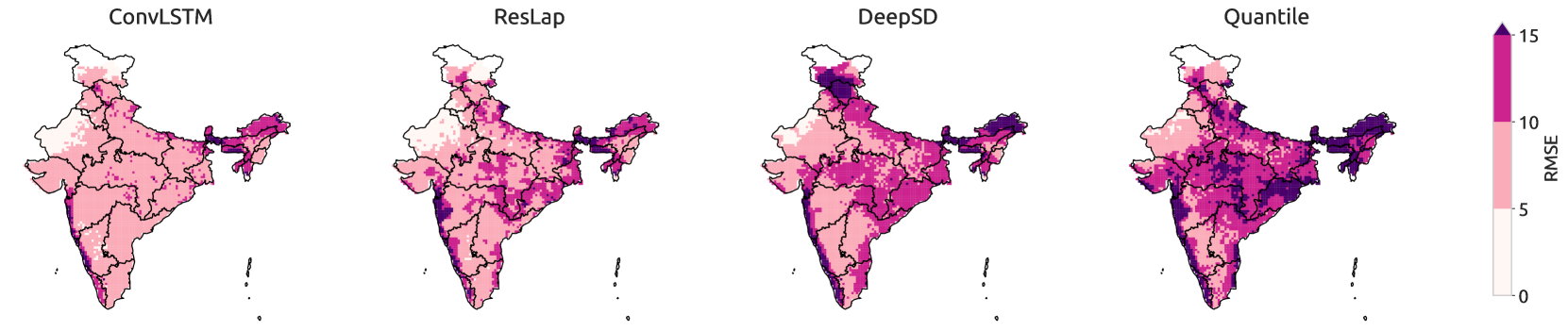
Figure 5. (Best viewed in color) Daily root-mean-square error (RMSE) computed for years between 2000–2005 (test set) for ConvLSTM, ResLap, DeepSD and Q-Map.

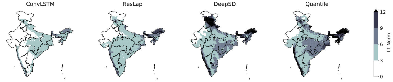
Figure 6. (Best viewed in color) L1 Norm computed on average projection for years between 2000–2005 (test set) for ConvLSTM, ResLap, DeepSD and Q-Map.

6.1. Daily Predictability

Results of Root mean square error (RMSE) of the predicted projections of precipitation over India during the months of monsoon and non-monsoon is shown in Fig 4. The difference in RMSE values of our method with that of ResLap and DeepSD over each location in India is given on the right-side in Fig 4. The lower rate of errors of our method on both monsoon and non-monsoon period over India shows the improved performance of ConvLSTM. Similarly, Fig 6 shows the projection of overall Root mean square error (RMSE) of the methods over the whole test set of precipitation (2000-2005). It can be clearly observed that despite ESM having false projections over East-part of India, the model generates more accurate projections over the southern part of India along with maintaining the extreme values.

The predictive performance of the model in terms of root-mean-square-error (RMSE) and Bias values on monsoon and non-monsoon are shown in Table 2. The model has performed remarkably well in the non-monsoon periods with a test accuracy of $2.37mm$, and even with the Monsoon period, model has performed well enough with test RMSE of $9.86mm$ despite the period having more extremes over the southern region with a large offset between the ESM and the observed data. Table 3 shows the overall predictive performance of the models on the whole test set (2000-2005). Table 4 shows a season-wise comparison of RMSE and Bias values. Again, it can be observed clearly that ConvLSTM outperforms the other methods for chosen metrics in all seasons.

Table 2. Performance of our proposed model against ResLap, DeepSD and Q-Map on the period of 2000-2005 (test data) for Monsoon and non-monsoon period

		Our	ResLap	DeepSD	Q-Map
Non Monsoon	RMSE	2.37	4.02	5.77	7.04
	Bias	0.79	1.23	4.18	1.94
Monsoon	RMSE	9.86	12.46	12.66	19.48
	Bias	5.18	6.23	7.15	9.99

Table 3. Overall Performance of our proposed model against ResLap, DeepSD and Q-Map on the period of 2000-2005 (test data) in India.

	Our	ResLap	DeepSD	Q-Map
RMSE	7.94	9.88	11.42	14.16
Bias	3.17	3.72	5.97	4.63

Table 4. Season-wise Performance of our proposed model against ResLap, DeepSD and Q-Map on the period of 2000-2005 (test data) in India.

		Our	ResLap	DeepSD	Q-Map
RMSE	DJF	2.38	3.31	6.69	6.45
	JJA	12.78	15.62	16.74	21.68
	MAM	4.03	5.07	7.30	8.15
	SON	8.32	10.39	11.92	14.36
Bias	DJF	0.64	1.15	4.07	0.98
	JJA	6.298	7.65	8.49	10.06
	MAM	1.36	1.60	4.21	1.94
	SON	3.61	4.45	6.60	5.12

6.2. Predicting Extremes

We perform various evaluations of the methods on extreme events of precipitation. For this, first we consider the precipitation events that are greater than the $90$th percentile for each location over the grid of India. We select the $25$th and the $75$th quantiles of both RMSE and Bias values for determining the confidence intervals. Fig 9 shows the plot of mean along with the computed confidence bounds of Root mean square error (RMSE) and Bias values on the percentile threshold between $90$ and $98$. It can be seen clearly that both ResLap and DeepSD overpredicts the precipitation values at the extremes and performs the worst. Q-map manages to lower the RMSE value on extremes for the monsoon-period, however, it is observed that it’s performance is not stable and produces high biased values on all the other periods. Even though RMSE and Bias values deviates much more on the extremes, however, ConvLSTM is able to maintain stable performance and overall still outperforms the other methods. We also construct quantile-quantile(Q-Q) plots to measure the overall performance of methods on extreme events. We select four random grid-points over India and we compare the quantiles generated by the methods with the quantile of the observed precipitation. Fig 7 shows the Q-Q plots on the four randomly chosen grid points. We also contruct Q-Q plot of the entire grid of India averaged over the test period. Fig 8 shows this average Q-Q plot. It can be observed that the quantiles of both DeepSD (Thomas Vandal, 2017) and ResLap (Cheng et al., 2020) deviates from the observation. The quantile produced by Q-map is closer for some grid points but it is has large deviation on other points. Our approach on the other hand, produces stable quantiles and on average, it has the closest quantiles with that of the observed projection.

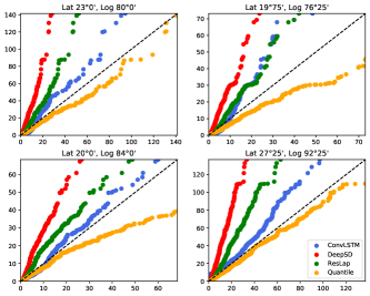
Figure 7. Quantile vs Quantile (Q-Q) plots on 4 randomly chosen grid points over India. The x-axis denotes the actual expected quantiles and y-axis denotes the quantiles produced by the methods.

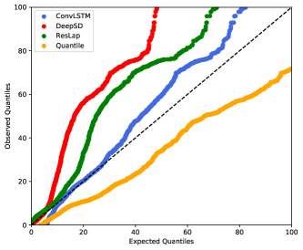
Figure 8. Quantile vs Quantile (qq) plot of the projection of grid points averaged over test period on India. The x-axis denotes the actual expected quantiles and y-axis denotes the quantiles produced by the methods.

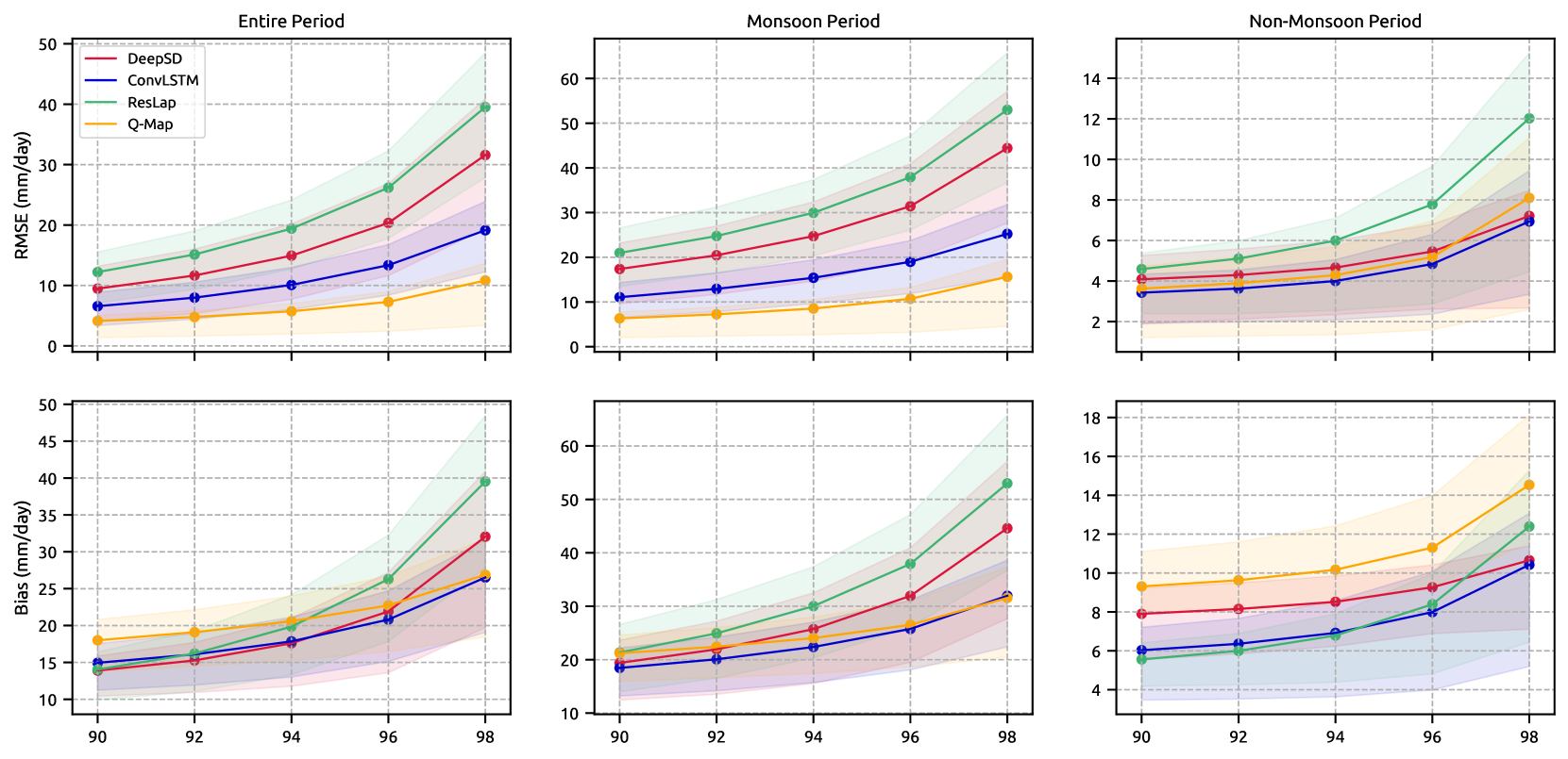
Figure 9. (Best viewed in color) Comparison of predictive performance on extreme precipitation of ConvLSTM, ResLap and DeepSD on the entire (a, d), monsoon (b, e) and non-monsoon (c, f) periods betweeen the year 2000-2005. At each location in India, all precipitation events above a percentile threshold (x-axis) are selected. Percentile thresholds between 90 and 99.9 are used. RMSE (a, b, c) and Bias (d, e, f) are computed for these events over India and averaged over the period for years 2000 to 2005 (test data). Confidence intervals show inter quantile range computed over entire India.

7. Conclusion

While state-of-the-Art Super-resolution architectures have shown promise for single image SD, ESMs models have complex spatiotemporal dependencies that need to be accounted for explicitly. Second, Due to a high computational cost associated with ConvLSTMs, the effective sequence length (the number of days to be included as lag variables) that could be used as an input is limited by the computing resources available. Hence, future dependencies need to account for long term spatiotemporal variability in addition to near-term dependencies, which is a typical characteristic of climate systems that shape up the atmospheric processes. Finally, handling non-stationarities (both in space and time) remains an open question in the field of SD. Future work needs to build on design-of-experiments strategies proposed by Salvi et. al  (Salvi et al., 2016) to evaluate the performance of SD approaches under non-stationary climate scenarios. We emphasize that while there has been growing interest of the scientific community in the applications of deep learning architectures in generating high-resolution outputs of Earth System Models, translation of these outputs to design relevant intensity, duration and frequency curves require more robust evaluation metrics of extremes which are stakeholder relevant.

REPRODUCIBILITY

We have utilized only free open-source scientific libraries and frameworks for the experiments. The coarse resolution precipitation data from NCAR Community Earth System Model (NCAR CESM1 CAM5) is available on climate model inter-comparison project (CMIP5) archives and auxilliary variables used as part of the study are available from UCAR NCAR repository. All codes used to generate these results are available on Github .

References

- (1)
- Abadi et al. (2016) Martín Abadi, Ashish Agarwal, Paul Barham, Eugene Brevdo, Zhifeng Chen, Craig Citro, Greg S. Corrado, Andy Davis, Jeffrey Dean, Matthieu Devin, Sanjay Ghemawat, Ian Goodfellow, Andrew Harp, Geoffrey Irving, Michael Isard, Yangqing Jia, Rafal Jozefowicz, Lukasz Kaiser, Manjunath Kudlur, Josh Levenberg, Dan Mane, Rajat Monga, Sherry Moore, Derek Murray, Chris Olah, Mike Schuster, Jonathon Shlens, Benoit Steiner, Ilya Sutskever, Kunal Talwar, Paul Tucker, Vincent Vanhoucke, Vijay Vasudevan, Fernanda Viegas, Oriol Vinyals, Pete Warden, Martin Wattenberg, Martin Wicke, Yuan Yu, and Xiaoqiang Zheng. 2016. TensorFlow: Large-Scale Machine Learning on Heterogeneous Distributed Systems. arXiv:cs.DC/1603.04467
- Adarsh and Reddy (2019) S Adarsh and M Janga Reddy. 2019. Links Between Global Climate Teleconnections and Indian Monsoon Rainfall. In Climate Change Signals and Response. Springer, 61–72.
- Arora et al. (2013) Vivek K Arora, George J Boer, Pierre Friedlingstein, Michael Eby, Chris D Jones, James R Christian, Gordon Bonan, Laurent Bopp, Victor Brovkin, Patricia Cadule, et al. 2013. Carbon–concentration and carbon–climate feedbacks in CMIP5 Earth system models. Journal of Climate 26, 15 (2013), 5289–5314.
- Bhatia and Ganguly (2019) Udit Bhatia and Auroop Ratan Ganguly. 2019. Precipitation extremes and depth-duration-frequency under internal climate variability. Scientific reports 9, 1 (2019), 1–9.
- Brenkert and Malone (2005) Antoinette L Brenkert and Elizabeth L Malone. 2005. Modeling vulnerability and resilience to climate change: a case study of India and Indian states. Climatic Change 72, 1-2 (2005), 57–102.
- Cannon (2011) Alex J Cannon. 2011. Quantile regression neural networks: Implementation in R and application to precipitation downscaling. Computers & geosciences 37, 9 (2011), 1277–1284.
- Cannon et al. (2015) Alex J Cannon, Stephen R Sobie, and Trevor Q Murdock. 2015. Bias correction of GCM precipitation by quantile mapping: how well do methods preserve changes in quantiles and extremes? Journal of Climate 28, 17 (2015), 6938–6959.
- Chen et al. (2010) Shien-Tsung Chen, Pao-Shan Yu, and Yi-Hsuan Tang. 2010. Statistical downscaling of daily precipitation using support vector machines and multivariate analysis. Journal of hydrology 385, 1-4 (2010), 13–22.
- Cheng et al. (2020) J. Cheng, Q. Kuang, C. Shen, J. Liu, X. Tan, and W. Liu. 2020. ResLap: Generating High-Resolution Climate Prediction Through Image Super-Resolution. IEEE Access 8 (2020), 39623–39634.
- Clift and Plumb (2008) Peter D Clift and R Alan Plumb. 2008. The Asian monsoon: causes, history and effects. Vol. 288. Cambridge University Press Cambridge.
- Dessai et al. (2009a) Suraje Dessai, Mike Hulme, Robert Lempert, and Roger Pielke Jr. 2009a. Climate prediction: a limit to adaptation. Adapting to climate change: thresholds, values, governance (2009), 64–78.
- Dessai et al. (2009b) Suraje Dessai, Mike Hulme, Robert Lempert, and Roger Pielke Jr. 2009b. Do we need better predictions to adapt to a changing climate? Eos, Transactions American Geophysical Union 90, 13 (2009), 111–112.
- Dong et al. (2014a) Chao Dong, Chen Change Loy, Kaiming He, and Xiaoou Tang. 2014a. Image Super-Resolution Using Deep Convolutional Networks. arXiv:cs.CV/1501.00092
- Dong et al. (2014b) Chao Dong, Chen Change Loy, Kaiming He, and Xiaoou Tang. 2014b. Learning a deep convolutional network for image super-resolution. In European conference on computer vision. Springer, 184–199.
- Faghmous and Kumar (2014) James H Faghmous and Vipin Kumar. 2014. A big data guide to understanding climate change: The case for theory-guided data science. Big data 2, 3 (2014), 155–163.
- Gadgil and Gadgil (2006) Sulochana Gadgil and Siddhartha Gadgil. 2006. The Indian monsoon, GDP and agriculture. Economic and Political Weekly (2006), 4887–4895.
- Ghosh and Mujumdar (2008) Subimal Ghosh and Pradeep P Mujumdar. 2008. Statistical downscaling of GCM simulations to streamflow using relevance vector machine. Advances in water resources 31, 1 (2008), 132–146.
- Guo et al. (2012) Jing Guo, Hua Chen, Chong-Yu Xu, Shenglian Guo, and Jiali Guo. 2012. Prediction of variability of precipitation in the Yangtze River Basin under the climate change conditions based on automated statistical downscaling. Stochastic Environmental Research and Risk Assessment 26, 2 (2012), 157–176.
- Hansen et al. (1983) J Hansen, G Russell, D Rind, P Stone, A Lacis, S Lebedeff, R Ruedy, and L Travis. 1983. Efficient three-dimensional global models for climate studies: Models I and II. Monthly Weather Review 111, 4 (1983), 609–662.
- Kalnay et al. (1996) Eugenia Kalnay, Masao Kanamitsu, Robert Kistler, William Collins, Dennis Deaven, Lev Gandin, Mark Iredell, Suranjana Saha, Glenn White, John Woollen, et al. 1996. The NCEP/NCAR 40-year reanalysis project. Bulletin of the American meteorological Society 77, 3 (1996), 437–472.
- Kay et al. (2015) Jennifer E Kay, Clara Deser, A Phillips, A Mai, Cecile Hannay, Gary Strand, Julie Michelle Arblaster, SC Bates, Gokhan Danabasoglu, J Edwards, et al. 2015. The Community Earth System Model (CESM) large ensemble project: A community resource for studying climate change in the presence of internal climate variability. Bulletin of the American Meteorological Society 96, 8 (2015), 1333–1349.
- Kingma and Ba (2014) Diederik P. Kingma and Jimmy Ba. 2014. Adam: A Method for Stochastic Optimization. arXiv:cs.LG/1412.6980
- Kulkarni et al. (2009) Ashwini Kulkarni, SS Sabade, and RH Kripalani. 2009. Spatial variability of intra-seasonal oscillations during extreme Indian monsoons. International Journal of Climatology: A Journal of the Royal Meteorological Society 29, 13 (2009), 1945–1955.
- Kumar and Ganguly (2018) Devashish Kumar and Auroop R Ganguly. 2018. Intercomparison of model response and internal variability across climate model ensembles. Climate dynamics 51, 1-2 (2018), 207–219.
- Lai et al. (2017) W. Lai, J. Huang, N. Ahuja, and M. Yang. 2017. Deep Laplacian Pyramid Networks for Fast and Accurate Super-Resolution. In 2017 IEEE Conference on Computer Vision and Pattern Recognition (CVPR). 5835–5843.
- Lai et al. (2017) Wei-Sheng Lai, Jia-Bin Huang, Narendra Ahuja, and Ming-Hsuan Yang. 2017. Deep Laplacian Pyramid Networks for Fast and Accurate Super-Resolution. In IEEE Conferene on Computer Vision and Pattern Recognition.
- Lauritzen et al. (2018) Peter Hjort Lauritzen, Ram D Nair, AR Herrington, P Callaghan, S Goldhaber, JM Dennis, JT Bacmeister, BE Eaton, CM Zarzycki, Mark A Taylor, et al. 2018. NCAR release of CAM-SE in CESM2. 0: A reformulation of the spectral element dynamical core in dry-mass vertical coordinates with comprehensive treatment of condensates and energy. Journal of Advances in Modeling Earth Systems 10, 7 (2018), 1537–1570.
- Mishra et al. (2012) Vimal Mishra, Brian V Smoliak, Dennis P Lettenmaier, and John M Wallace. 2012. A prominent pattern of year-to-year variability in Indian Summer Monsoon Rainfall. Proceedings of the National Academy of Sciences 109, 19 (2012), 7213–7217.
- Misra et al. (2017) Saptarshi Misra, Sudeshna Sarkar, and Pabitra Mitra. 2017. Statistical downscaling of precipitation using long short-term memory recurrent neural networks. Theoretical and Applied Climatology 134 (11 2017), 1–18. https://doi.org/10.1007/s00704-017-2307-2
- Misra et al. (2018) Saptarshi Misra, Sudeshna Sarkar, and Pabitra Mitra. 2018. Statistical downscaling of precipitation using long short-term memory recurrent neural networks. Theoretical and Applied Climatology 134, 3-4 (2018), 1179–1196.
- Nair and Hinton (2010) Vinod Nair and Geoffrey E. Hinton. 2010. Rectified Linear Units Improve Restricted Boltzmann Machines. In Proceedings of the 27th International Conference on International Conference on Machine Learning (ICML’10). Omnipress, Madison, WI, USA, 807–814.
- Pai et al. (2014) DS Pai, Latha Sridhar, M Rajeevan, OP Sreejith, NS Satbhai, and B Mukhopadhyay. 2014. Development of a new high spatial resolution (0.25 0.25) long period (1901–2010) daily gridded rainfall data set over India and its comparison with existing data sets over the region. Mausam 65, 1 (2014), 1–18.
- Prein et al. (2017) Andreas F Prein, Roy M Rasmussen, Kyoko Ikeda, Changhai Liu, Martyn P Clark, and Greg J Holland. 2017. The future intensification of hourly precipitation extremes. Nature Climate Change 7, 1 (2017), 48–52.
- Salvi et al. (2016) Kaustubh Salvi, Subimal Ghosh, and Auroop R Ganguly. 2016. Credibility of statistical downscaling under nonstationary climate. Climate Dynamics 46, 5-6 (2016), 1991–2023.
- Schmidt (2010) Gavin Schmidt. 2010. THE REAL HOLES IN CLIMATE SCIENCE. Nature 463 (2010), 21.
- Shi et al. (2015) Xingjian Shi, Zhourong Chen, Hao Wang, Dit-Yan Yeung, Wai kin Wong, and Wang chun Woo. 2015. Convolutional LSTM Network: A Machine Learning Approach for Precipitation Nowcasting. arXiv:cs.CV/1506.04214
- Shocher et al. (2018) Assaf Shocher, Nadav Cohen, and Michal Irani. 2018. “zero-shot” super-resolution using deep internal learning. In Proceedings of the IEEE Conference on Computer Vision and Pattern Recognition. 3118–3126.
- Taylor et al. (2012) Karl E Taylor, Ronald J Stouffer, and Gerald A Meehl. 2012. An overview of CMIP5 and the experiment design. Bulletin of the American Meteorological Society 93, 4 (2012), 485–498.
- Thomas Vandal (2017) Auroop R Ganguly Thomas Vandal, Evan Kodra. 2017. DeepSD: Generating High Resolution Climate Change Projections through Single Image Super-Resolution. In proceedings of SIGKDD Conference on Knowledge Discovery and Data Mining (KDD), ACM, 1663–1672. https://doi.org/10.1145/3097983.3098004
- Vandal et al. (2017) Thomas Vandal, Evan Kodra, Sangram Ganguly, Andrew Michaelis, Ramakrishna Nemani, and Auroop R Ganguly. 2017. Deepsd: Generating high resolution climate change projections through single image super-resolution. In Proceedings of the 23rd acm sigkdd international conference on knowledge discovery and data mining. 1663–1672.
- Wilby and Dessai (2010) Robert L Wilby and Suraje Dessai. 2010. Robust adaptation to climate change. Weather 65, 7 (2010), 180–185.
- Wilby and Wigley (1997) Robert L Wilby and TML Wigley. 1997. Downscaling general circulation model output: a review of methods and limitations. Progress in physical geography 21, 4 (1997), 530–548.
- Xingjian et al. (2015) SHI Xingjian, Zhourong Chen, Hao Wang, Dit-Yan Yeung, Wai-Kin Wong, and Wang-chun Woo. 2015. Convolutional LSTM network: A machine learning approach for precipitation nowcasting. In Advances in neural information processing systems. 802–810.
- Xu et al. (2018) J. Xu, Y. Chae, B. Stenger, and A. Datta. 2018. Dense Bynet: Residual Dense Network for Image Super Resolution. In 2018 25th IEEE International Conference on Image Processing (ICIP). 71–75.
- Xue et al. (2014) Yongkang Xue, Zavisa Janjic, Jimy Dudhia, Ratko Vasic, and Fernando De Sales. 2014. A review on regional dynamical downscaling in intraseasonal to seasonal simulation/prediction and major factors that affect downscaling ability. Atmospheric research 147 (2014), 68–85.
- Yuan et al. (2013) Naiming Yuan, Zuntao Fu, and Shida Liu. 2013. Long-term memory in climate variability: A new look based on fractional integral techniques. Journal of Geophysical Research: Atmospheres 118, 23 (2013), 12–962.
- Zhang et al. (2013) Xuebin Zhang, Hui Wan, Francis W Zwiers, Gabriele C Hegerl, and Seung-Ki Min. 2013. Attributing intensification of precipitation extremes to human influence. Geophysical Research Letters 40, 19 (2013), 5252–5257.
- Zhang et al. (2018) Yulun Zhang, Yapeng Tian, Yu Kong, Bineng Zhong, and Yun Fu. 2018. Residual dense network for image super-resolution. In Proceedings of the IEEE conference on computer vision and pattern recognition. 2472–2481.