Efficient early stellar feedback can suppress galactic outflows by reducing supernova clustering

Abstract

We present a novel set of stellar feedback models, implemented in the moving-mesh code Arepo, designed for galaxy formation simulations with near-parsec (or better) resolution. These include explicit sampling of stars from the IMF, allowing feedback to be linked to individual massive stars, an improved method for the modelling of H ii regions, photoelectric heating from a spatially varying FUV field and supernova feedback. We perform a suite of 32 simulations of isolated $M_{\mathrm{vir}}=10^{10}\,\mathrm{M_{\odot}}$ galaxies with a baryonic mass resolution of $20\,\mathrm{M_{\odot}}$ in order to study the non-linear coupling of the different feedback channels. We find that photoionization and supernova feedback are both independently capable of regulating star formation to the same level, while photoelectric heating is inefficient. Photoionization produces a considerably smoother star formation history than supernovae. When all feedback channels are combined, the additional suppression of star formation rates is minor. However, outflow rates are substantially reduced relative to the supernova only simulations. We show that this is directly caused by a suppression of supernova clustering by the photoionization feedback, disrupting star forming clouds prior to the first supernovae. We demonstrate that our results are robust to variations of our star formation prescription, feedback models and the baryon fraction of the galaxy. Our results also imply that the burstiness of star formation and the mass loading of outflows may be overestimated if the adopted star particle mass is considerably larger than the mass of individual stars because this imposes a minimum cluster size.

1 Introduction

It is well established that the process of galaxy formation and evolution cannot solely be captured by the physics of gravitational collapse, hydrodynamics and radiative cooling. Star formation in galaxies is significantly less efficient than such a naive determination would predict (see e.g. Zuckerman & Evans II 1974; Williams & McKee 1997; Kennicutt 1998; Evans 1999; Krumholz & Tan 2007; Evans et al. 2009). The interstellar medium (ISM) is observed to have a complex phase structure (see e.g. the review of Ferrière 2001) originating from a variety of sources of heating as well as cooling. The baryon fractions of galaxies far exceed those of observations unless some mechanism mitigates the flow of gas into haloes (White & Frenk 1991; Springel & Hernquist 2003b; Kereš et al. 2009). Indeed, an ejection of mass out of the star forming regions of galaxies is required in order to explain the metal enrichment of the surrounding circumgalactic medium (CGM) (Aguirre et al. 2001; Pettini et al. 2003; Songaila 2005, 2006; Martin et al. 2010). This mass transfer is observed in the form of multi-phase galactic outflows travelling at hundreds of $\mathrm{km\,s^{-1}}$ (see e.g. Martin 1999, 2005; Veilleux et al. 2005) with mass flow rates that match or exceed the star formation rate (SFR) of the galaxy (Bland-Hawthorn et al. 2007; Schroetter et al. 2015). The phenomena described above in broad strokes (as well as many others) can be explained to a greater or lesser degree by the inclusion of feedback processes, originating from stars or active galactic nuclei (AGN), into theories of galaxy formation. This approach has driven significant progress in the field (see e.g. the review of Somerville & Davé 2015). AGN feedback is believed to operate primarily in galaxies more massive than the Milky Way while stellar feedback dominates in lower mass galaxies (although there have been recent observational and theoretical suggestions that AGN feedback may also operate in lower mass galaxies, see e.g. Silk 2017; Dashyan et al. 2018; Penny et al. 2018; Koudmani et al. 2019; Koudmani et al. 2021; Manzano-King et al. 2019).

Perhaps the most commonly invoked form of stellar feedback is the injection of mass, energy and momentum by supernovae (SNe). The ability of SNe to determine the phase structure of the ISM has been acknowledged for some time (McKee & Ostriker 1977). There is also an established theoretical basis for predicting the regulation of star formation efficiencies (SFE) by SN–driven ISM turbulence (Ostriker et al. 2010; Ostriker & Shetty 2011; Kim et al. 2011; Faucher-Giguere et al. 2013; Hayward & Hopkins 2017), although other studies show that the SFE within giant molecular clouds (GMCs) is reduced to the percent level prior to the first SN by cloud turbulence, magnetic fields, stellar winds and jets (see e.g. Federrath 2015; Grudić et al. 2018). It has been known for decades that SNe are able to drive galactic outflows (Chevalier & Clegg 1985).

The aforementioned ability of SN feedback to regulate the ISM, star formation and drive outflows has been incorporated into numerical hydrodynamic simulations of galaxy formation at various levels of abstraction depending on the resolution available. When the ISM is entirely unresolved (e.g. in large volume cosmological simulations), sub-grid models with a high level of abstraction must be adopted, typically involving a modification of the equation of state of ISM gas and the use of phenomenological models for the generation of galactic outflows (Springel & Hernquist 2003a; Vogelsberger et al. 2013; Vogelsberger et al. 2014; Dubois et al. 2014; Dubois et al. 2016; Schaye et al. 2015; Davé et al. 2016; Davé et al. 2019; Pillepich et al. 2018). When the ISM can be marginally resolved (with mass resolutions of $10^{2}-10^{4}\,\mathrm{M_{\odot}}$), typically because individual galaxies are being simulated, more explicit sub-grid models can be used (see e.g. Hopkins et al. 2014; Ceverino et al. 2014; Kimm et al. 2015; Agertz & Kravtsov 2015; Marinacci et al. 2019). When low mass galaxies are simulated, the spatial resolution reached can be on the order of a parsec or better (see e.g. Hu et al. 2017; Hu 2019; Smith et al. 2018; Emerick et al. 2019, 2020; Agertz et al. 2020). Dwarf galaxies provide a useful laboratory for studying stellar feedback because their shallow potential well makes them very sensitive to it. Finally, the highest resolutions are reached in simulations of patches of galaxies (see e.g. Hennebelle & Iffrig 2014; Walch et al. 2015; Gatto et al. 2015; Li et al. 2015; Kim & Ostriker 2015b, 2017; Martizzi et al. 2016 and the compilation of Li & Bryan 2020). These simulations permit the modelling of SN feedback in an explicit manner, allowing the creation of a multi-phase, turbulent ISM and the driving of outflows to arise naturally without relying on sub-grid models.

Recently, it has become apparent that the clustering of SNe in both space and time has a non-trivial impact on their ability to drive galactic outflows. When SNe occur close together, their blast waves overlap and form “superbubbles”. Idealized simulations studying the generation and behaviour of these superbubbles in 1D (Sharma et al. 2014; Gentry et al. 2017; El-Badry et al. 2019) and 3D (Yadav et al. 2017; Gentry et al. 2019) have demonstrated that the net impact of SNe is greatly enhanced when they occur in clusters as opposed to isolation. Due to their vulnerability to radiative losses, isolated SNe are unable to create a hot ISM phase and their main contribution is to couple momentum into the ISM (which is also reduced relative to the clustered case). When SNe are clustered such that successive SNe occur approximately within a cooling time and length of each other, a hot bubble can be maintained and momentum input is enhanced. Experiments in a galactic context (Fielding et al. 2017, 2018; Martizzi 2020) support this picture, but also highlight the role of superbubble breakout in the efficient driving of winds. Crucially, SN remnants (SNRs) must be able to make their way out of the dense gas of the galactic disc in order to couple mass and energy into the CGM. Isolated SNe typically radiate too much energy away pre-breakout. Clustered SNe, on the other hand, are able to work together to inflate superbubbles that can reach breakout while retaining a substantial fraction of their initial energy. The gas in the superbubble (as well as the SNRs of subsequent SNe) can vent straight into the CGM, bypassing the ISM, allowing the creation of highly energetic winds with mass loadings of unity or higher. This venting also has implications for the metal loading of the winds, since mixing of SN ejecta with the ISM is reduced.

SNe are not the only form of stellar feedback. Winds from massive stars are capable of creating cavities in star forming clouds (see e.g. Dale et al. 2014; Gallegos-Garcia et al. 2020) prior to the first SNe. The energy budget contained in radiation from massive stars far outstrips that produced by SNe (Leitherer et al. 1999), although the manner in which they couple this energy to the ISM is more complicated. Photoionization, photoheating and radiation pressure from massive stars (forming H ii regions) can significantly disrupt giant molecular clouds prior to the first SNe (Vázquez-Semadeni et al. 2010; Walch et al. 2012; Dale et al. 2014; Sales et al. 2014) although the ability of radiation pressure to drive galactic outflows is disputed (see e.g. the discussion in Rosdahl et al. 2015). Photoelectric heating caused by FUV radiation plays a role in setting the state of the ISM (see e.g. Wolfire et al. 2003) and regulating SFRs, although the impact of this effect in dwarf galaxies (Forbes et al. 2016; Hu et al. 2016, 2017; Emerick et al. 2019) varies depending on the amount of dust present. The production of photodissociating Lyman-Werner photons regulates the mass fraction of H₂ in the ISM (see e.g. Hu et al. 2016; Emerick et al. 2019). Momentum coupled into the ISM by the resonant scattering of Ly$\alpha$ photons may play a non-negligible role in metal-poor galaxies (Kimm et al. 2018). Feedback from high-mass X-ray binaries (HMXBs) can influence the ISM in a complex manner (Artale et al. 2015; Garratt-Smithson et al. 2018, 2019). Because all of these different feedback processes operate on different timescales and have complex dependencies on the state of the ambient ISM, they interact in a highly non-linear fashion. This means that the question “which feedback channel is the most important?” is often not well posed.

Nonetheless, it is usually a reasonable assessment that SNe are the primary driver of galactic outflows (in the absence of an AGN). The role of the other forms of stellar feedback in outflow driving are then often considered in terms of the way they assist or impede the SNe. Perhaps the most commonly invoked interaction is the enhancement of outflow driving efficiency by dropping the local gas density before SNe occur. Enhancement of outflow rates can also occur if pre-SN feedback clears channels out of the disc, making breakout easier. However, while it is mentioned less frequently, it is also possible for pre-SN feedback to reduce the efficiency of SN outflow driving. If the SFR is regulated down to a lower level, then the SN rate similarly drops. A more subtle interaction occurs if the pre-SN feedback alters the clustering properties of the SNe, reducing their ability to form superbubbles. This phenomenon will be a particular focus of this work.

This work was carried out as part of the SMAUG (Simulating Multiscale Astrophysics to Understand Galaxies) project. The aims of the SMAUG project are to develop and implement a new set of sub-grid models for use in large volume cosmological simulations. These models will have their basis in knowledge gained from high resolution simulations that explicitly resolve small-scale physics, rather than being tuned to large scale observables. To this end, the SMAUG consortium is carrying out a diverse range of numerical experiments across a variety of spatial scales to study the key physical processes involved in galaxy formation in detail (Li et al. 2020a, b; Kim et al. 2020a, b; Motwani et al. 2020; Fielding et al. 2020; Pandya et al. 2020; Anglés-Alcázar et al. 2020). This work forms a part of that effort.

2 A guide to this work

This work necessarily contains both a detailed description of our new numerical schemes as well as an in-depth presentation of their application. We acknowledge that readers may wish to omit parts of the paper, for example, skipping the detailed numerical methods section. Therefore, for the convenience of the reader, we now outline the key points of the work and where they can be found.

• In Section 3 we present a new set of sub-grid models for modelling star formation and stellar feedback implemented in the code Arepo. Section 3.2 details our adopted star formation criteria and explicit IMF sampling scheme, by which we are able to keep track of individual massive stars in the simulation. Section 3.3 presents our models for stellar feedback. These include a model for photoelectric heating using a spatially varying interstellar radiation field, a novel scheme for modelling overlapping H ii regions that accounts for anisotropic distributions of neutral gas and our SN feedback scheme.

• Section 4 details the initial conditions used in this work, comprising of 3 high resolution isolated $M_{\mathrm{vir}}=10^{10}\,\mathrm{M_{\odot}}$ systems with differing baryon fractions. Table 1 is a reference for the 32 simulations presented in this work and the various combinations of initial conditions, stellar feedback channels and other parameter variations used.

• Sections 5.1-5.4 explore basic galaxy properties for our fiducial six simulations. We show that the addition of photoionization feedback provides smooth SFRs and significantly suppresses the generation of outflows by SNe. In Section 5.5 we show that this is because the photoionization feedback significantly reduces the clustering of SNe.

• In Section 5.6 we demonstrate that while different star formation prescriptions do alter the degree of SN clustering, this is subdominant to the impact of ionizing radiation.

• In Section 6 we discuss the limitations of our photoionization feedback model, the non-linear and non-monotonic consequences of combining different feedback channels, the implications of our findings for coarser resolution simulations and compare our results to other works. We also discuss whether it is necessary to invoke additional physics that are missing from our simulations to compensate for the de-clustering ability of efficient pre-SN feedback.

• Section 7 contains our concluding remarks.

• Appendix A shows that our results are insensitive to increasing or decreasing the baryon fraction of our galaxy by a factor of two. In Appendix B we explore why photoelectric heating is almost always inefficient in our simulations and examine the sensitivity to the dust-to-gas ratio, local shielding approximation and the assumed heating efficiency. In Appendix C we demonstrate the robustness of our short-range photoionization model. In Appendix D we test a model for treating long-range ionizing radiation that assumes all attenuation occurs locally and argue that it is not a suitable substitute for full RT in this context, despite its recent adoption by other groups.

3 Numerical methods

3.1 Gravity, hydrodynamics and cooling

We use the code Arepo (Springel 2010; Pakmor et al. 2016) in combination with our own novel extensions to model star formation and stellar feedback (described in subsequent sections). Hydrodynamics are included with a quasi-Lagrangian finite volume scheme, which makes use of an unstructured moving-mesh based on a Voronoi tessellation of discrete mesh-generating points that are drifted with the local gas velocity. Gravity is included with a tree-based algorithm. We use the Grackle chemistry and cooling library (Smith et al. 2017) in its non-equilibrium six-species mode (H i, H ii, He i, He ii, He iii and electrons), tracking the advection of these species with our hydrodynamical scheme. Grackle also provides metal cooling via look-up tables computed using the photoionization simulation code Cloudy (Ferland et al. 2013). Cooling rates are tabulated as a function of total metallicity (i.e. not broken into individual elements) and scaled relative to local metallicity assuming a solar abundance pattern. We therefore also track the advection of a global metallicity field. In this work we do not track the abundances of individual metal species separately, but this is possible with our schemes. We include ionization and heating from a metagalactic UV background (Haardt & Madau 2012). We include self-shielding from the UV background by using the implementation of a Rahmati et al. (2013) style prescription included in Grackle (including the corrected metal cooling tables). We adopt the version of the implementation recommended by Smith et al. (2017), where self-shielding is approximated in H i and He i but He ii ionization and heating is ignored.

3.2 Star formation

3.2.1 Determining the local star formation rate

Due to the large dynamic range in spatial scales required to correctly treat star formation from first principles, in common with all other galaxy formation simulations, we must adopt some form of sub-grid model to capture the relevant processes that cannot be resolved. Our fiducial model is as follows. We identify star forming gas in the simulation as that which is unstable to gravitational collapse, specifically that which we only marginally resolve correctly with our gravito-hydrodynamic scheme. We therefore determine the local Jeans mass for each cell,

$$M_{\mathrm{J}}=\frac{\pi^{5/2}c_{\mathrm{s}}^{3}}{6G^{3/2}\rho^{1/2}},$$ (1)

where $c_{\mathrm{s}}$ and $\rho$ are the sound speed and density of the cell and $G$ is the gravitational constant. When $M_{\mathrm{J}}<N_{\mathrm{J}}m_{\mathrm{cell}}$, where $N_{\mathrm{J,SF}}$ is a free parameter and $m_{\mathrm{cell}}$ is the cell mass, we permit star formation in the cell. We adopt the value of $N_{\mathrm{J,SF}}=8$, used in a similar scheme by Hu et al. (2017). A detailed investigation into this choice is beyond the scope of this work, although we briefly examine the impact of changing this criteria in Section 5.6, along with the consequences of adopting an additional high density threshold, $n_{\mathrm{SF}}$.

For gas that meets this criteria, we calculate a local star formation rate using a simple Schmidt law, which assumes that the star formation rate proceeds on a local free-fall time, $t_{\mathrm{ff}}=\sqrt{3\pi/32G\rho}$, modulated by some efficiency, $\epsilon_{\mathrm{SF}}$:

$$\dot{\rho}_{\star}=\epsilon_{\mathrm{SF}}\frac{\rho}{t_{\mathrm{ff}}}.$$ (2)

For this work, we adopt a fixed value of $\epsilon_{\mathrm{SF}}=0.02$, motivated by observed efficiencies in dense gas (see e.g. Krumholz & Tan 2007, and references therein). In Section 5.6, we investigate the impact of using $\epsilon_{\mathrm{SF}}=1$ on our fiducial model. We intend to make a more detailed study of the consequences of different choices of $\epsilon_{\mathrm{SF}}$ in the future, as well as examining the use of models that vary efficiency as a function of local gas properties (e.g. levels of turbulence).

3.2.2 Explicit IMF sampling

The star formation rates are then used to stochastically convert gas cells into collisionless “star particles”. In many simulations, these particles are treated as single stellar populations (SSPs) with all resulting stellar feedback treated as an average over the population. This approach can be seen to be valid when the star particle mass is large enough that the distribution of stellar masses, specified by the initial mass function (IMF), is well sampled. Even when the star particle mass is small, this approach can still be used under the assumption that the IMF is still well sampled across the various star particles in the simulation as a whole (except in cases of very low star formation). However, when the star particle mass approaches that of individual stars one can improve upon this method by explicitly sampling the IMF and assigning individual stars to the star particles (see e.g. Hu et al. 2017; Hu 2019; Emerick et al. 2019). This allows the clustering of stellar feedback sources to be captured self-consistently, an option which is not available for lower resolution simulations. A companion paper to this work (Smith 2021) demonstrates that the effectiveness of photoionization feedback can be unphysically modulated if star particles are assigned an IMF averaged luminosity because the spatial and temporal distribution of rare, bright sources (which dominate the ionizing photon budget) is not correctly captured. We therefore adopt the explicit IMF sampling approach in this work. A detailed description of our implementation can be found in Smith (2021) but we give the salient details here.

Each star particle in the simulation represents a collection of discrete stars. We record the initial stellar inventory of each star particle and the overall stellar feedback produced by a particle is tied to its extant constituent stars (see Section 3.3 for details). When a gas cell is converted into a star particle, we sample the IMF to draw individual stellar masses with which we can populate its stellar inventory. In this work, we adopt a Kroupa (2001) IMF over the range $0.08-100\,\mathrm{M_{\odot}}$. The sampling is performed using an acceptance-rejection method with a power-law envelope function.

Ideally, we would like to draw samples until the total mass drawn, $M_{\mathrm{IMF}}$, equals the dynamical mass of the star particle, $m_{\mathrm{part}}$. Of course, discrete draws from the IMF are extremely unlikely to result in $M_{\mathrm{IMF}}=m_{\mathrm{part}}$, with an overshoot being inevitable. We accept the last drawn stellar mass in order to avoid biasing the IMF and assign the drawn population to the star particle. However, this obviously does not conserve mass. We resolve this discrepancy by requiring that when populating the next newly created star particle we aim for a correspondingly lower total inventory mass than its dynamical mass. Again, we draw until we overshoot the target. The discrepancy between this particle’s $M_{\mathrm{IMF}}$ and $m_{\mathrm{part}}$ is then used to set the target sample mass for the next particle and so on. The result is that for some particles $M_{\mathrm{IMF}}>m_{\mathrm{part}}$, while other particles will have $M_{\mathrm{IMF}}<m_{\mathrm{part}}$. However, the assigned and dynamical masses will be consistent when averaged across multiple particles. Note that this scheme makes it possible to, for example, assign a $40\,\mathrm{M_{\odot}}$ star to a $20\,\mathrm{M_{\odot}}$ star particle; the scheme compensates by not assigning any stars to the next formed star particle(s). Smith (2021) provides a greater discussion of the algorithm and its consequences, to which we refer the interested reader. Crucially, it demonstrates that other techniques commonly adopted to resolve the overshoot issue (e.g. stop-before, stop-after and stop-nearest) bias the IMF and the resultant stellar feedback budget to a non-negligible extent when $m_{\mathrm{part}}\lesssim 500\,\mathrm{M_{\odot}}$.

Our scheme is conceptually similar to that used in Hu et al. (2017), except that in their implementation dynamical mass is subsequently exchanged between star particles to enforce $M_{\mathrm{IMF}}=m_{\mathrm{part}}$ at the individual particle level. We instead accept the resulting inconsistency between the mass of the stars assigned to the star particle (used to determine the resulting stellar feedback) and its dynamical mass, preferring to avoid unphysical displacement of mass. This inconsistency is typically small at our chosen resolution of $20\,\mathrm{M_{\odot}}$ (except in the case of a very massive star being drawn, as discussed later). Any dynamical effects of this inconsistency are negligible since we already cannot follow exact N-body dynamics in this type of simulation.

3.3 Stellar feedback

3.3.1 Stellar properties

Emerick et al. (2019) derived far-UV (FUV) and ionizing photon luminosities as a function of a star’s mass and metallicity from the OSTAR2002 grid of stellar models (Lanz & Hubeny 2003), making use of a black body spectrum for masses outside the grid range (see the work for exact details). They assume no evolution in the spectral properties with time, instead fixing them to their zero age main sequence (MS) values. This approximation is reasonable since these luminosities typically do not change significantly during the MS phase, while the pre- and post-MS phases are short relative to the already rapid MS evolution. This approximation simplifies the implementation, removing the need to do an additional table interpolation as a function of age. However, a future scheme could incorporate time evolution if more detailed spectral properties were needed. We use this compiled data to assign FUV and ionizing photon luminosities to the star particles as the sum of the contributions from the individual (extant) stars that they contain. For simplicity, in this work we use the $0.1\,\mathrm{Z_{\odot}}$ luminosities for all stars, equal to that of the gas in the initial conditions (see below), rather than interpolating between metallicities. In reality, the luminosities do not have a strong dependence on metallicity, nor does the metallicity in the non-cosmological simulations presented below deviate far enough from the initial conditions for this to have any impact.

Likewise, we obtain lifetimes for the stars as a function of mass from the PARSEC grid of stellar tracks (Bressan et al. 2012). If the age of a star particle exceeds the lifetime of one of the individual stars it contains, that star is considered dead. Dead stars no longer contribute FUV or ionizing photon luminosity to their host star particle. Additionally, if the star has a mass in the range $8-35\,\mathrm{M_{\odot}}$ it will trigger a SN event (see below for details). Star particles containing extant stars with masses greater than $5\,\mathrm{M_{\odot}}$ (i.e. those that can contribute to feedback) have their time-steps limited to a maximum of 0.1 Myr; in reality, their time-steps are usually much shorter, as set by other constraints (e.g. the gravitational acceleration time-step). Finally, it should be noted that we do not account for binary stellar evolution nor runaway OB stars in this work.

3.3.2 Photoelectric heating

In galaxies with a dust-to-gas ratio (DGR) similar to Milky Way values, calculating the interstellar radiation field (ISRF) is made complex by dust extinction. However, in more dust-poor environments we can approximate the effects of extinction by assuming that it occurs locally with the majority of the medium between source and receiving location being optically thin. This makes the determination of the ISRF seen by each gas cell a simple inverse-square law summing of (locally attenuated) sources, in a manner similar to the gravity calculation. This approach is also taken by Forbes et al. (2016) and Hu et al. (2017) as well as being used in more dust rich environments in Hopkins et al. (2018b).

Relevant to photoelectric heating is the FUV luminosity in the range 6 - 13.6 eV. The luminosity of the star particle in this band, $L_{\mathrm{FUV},i}$, is the sum of the contributions from the individual stars assigned to it. The luminosity of the star particle is then attenuated with a Jeans length approximation,

$$L_{\mathrm{FUV,eff},i}=L_{\mathrm{FUV},i}\exp\left(-1.33\times 10^{-21}Dn\lambda_{\mathrm{J}}\right),$$ (3)

where $D$ is the DGR relative to the Milky Way, $n$ is the hydrogen nucleus number density and $\lambda_{J}$ is the Jeans length (in cgs units), all evaluated in the gas cell currently hosting the star particle. The DGR is calculated assuming a broken power-law dependency on gas metallicity taken from Rémy-Ruyer et al. (2014),

$$x=\mathrm{log}_{10}\left(\frac{Z}{0.014}\right),$$ (4)

$$\mathrm{log}_{10}\left(D\right)=\begin{cases}x,&x\geq-0.59\\ 3.1x+1.239,&x<-0.59\end{cases}$$ (5)

The radiation field strength at a given location, normalised to the Habing (1968) field, is then

$$G_{0}=\frac{1}{5.29\times 10^{-14}\,\mathrm{erg\,cm^{-3}}}\sum_{i}\frac{L_{\mathrm{FUV,eff},i}}{4\pi cr_{i}^{2}},$$ (6)

where the sum is carried out over all sources, $i$, a distance of $r_{i}$ from the location. This summation is carried out using the gravity tree, with sources softened in the same way as the gravitational force softening. Following Hu et al. (2017) we impose a minimum value for $G_{0}$ of $3.24\times 10^{-3}$, representing the contribution to the energy density between 6 - 13.6 eV from the $z=0$ UV background (Haardt & Madau 2012). The effective field strength seen by a gas cell after further local attenuation is

$$G_{\mathrm{eff}}=G_{0}\exp\left(-1.33\times 10^{-21}Dn\lambda_{\mathrm{J}}\right),$$ (7)

where the quantities are now evaluated in the receiving cell.

The cell now experiences a heating rate (which is passed to Grackle) of

$$\Gamma_{\mathrm{PE}}=1.3\times 10^{-24}\epsilon_{\mathrm{PE}}DG_{\mathrm{eff}}n\,\mathrm{erg\,s^{-1}\,cm^{-3}},$$ (8)

where $\epsilon_{\mathrm{PE}}$ is the photoelectric heating efficiency (Bakes & Tielens 1994; Wolfire et al. 2003; Bergin et al. 2004). The efficiency is properly a function of temperature and electron number density $n_{e}$ (e.g Wolfire et al. 2003). Unfortunately, obtaining an accurate determination of $n_{e}$ in the cold, dense ISM is extremely difficult since the major contributions come from carbon, dust and polyaromatic hydrocarbon (PAH) ionizations, additionally requiring a treatment of cosmic ray ionization. Erroneous photoelectric heating rates will result if these processes are not accurately modelled. Using a fixed value for $\epsilon_{\mathrm{PE}}$ is also undesirable since it can vary by over an order of magnitude across the range of densities and temperatures typical of the ISM. Instead, we follow the approach of Emerick et al. (2019) and allow $\epsilon_{\mathrm{PE}}$ to vary as a function of density. We use a fit to the results of Wolfire et al. (2003) (see fig. 10 of that work) for the solar neighbourhood (implicitly assuming the gas lies on the equilibrium curve),

$$\epsilon_{\mathrm{PE}}=\mathrm{MIN}\left[0.041,0.00871\left(n/\mathrm{cm^{-3}}\right)^{0.235}\right].$$ (9)

3.3.3 Short-range photoionization

We employ an overlapping Strömgren type approximation to model the effects of photoionization as is often employed in simulations without explicit radiative transfer (see e.g. Hopkins et al. 2018b; Hu et al. 2017). However, we improve upon typical schemes to account for anisotropic distributions of neutral gas. In a manner analogous to our scheme for photoelectric heating, we obtain the rate of ionizing photons, $S_{*,i}$, emitted from each star particle, $i$, as the sum of the contributions from the individual stars assigned to it. The rate of ionizing photons needed to balance recombinations in a gas cell, $j$, is $R_{\mathrm{rec},j}=\beta m\rho(X_{\mathrm{H}}/m_{\mathrm{p}})^{2}$, where $\beta=2.56\times 10^{-13}\,\mathrm{cm^{3}\,s^{-1}}$ is the case B recombination coefficient at $10^{4}\,\mathrm{K}$, $m_{\mathrm{p}}$ is the proton mass and $m$, $\rho$ and $X_{\mathrm{H}}$ are the mass, density and hydrogen mass fraction of the cell, respectively. If the cell is above a threshold temperature, $T_{\mathrm{photo,max}}$, such that it is sufficiently hot to be collisionally ionized, it is assigned $R_{\mathrm{rec},j}=0$. We adopt $T_{\mathrm{photo,max}}=1.05\times 10^{4}\,\mathrm{K}$, chosen to be slightly higher than our photoionization heating temperature (see later) to avoid numerical issues with cells ‘flipping’ in and out of H ii regions. However, results are largely insensitive to this value. Similarly, we ignore gas less dense than some threshold $n_{\mathrm{photo,min}}$, again assigning $R_{\mathrm{rec},j}=0$ for the purposes of our method. If the H ii region manages to break out into low density gas, it has essentially transitioned from being ionization bounded to being density bounded. The Strömgren approximation breaks down in low density gas. The timescale on which the Strömgren sphere evolves is the recombination time, $\tau\approx\left(\alpha_{\mathrm{H}}n_{\mathrm{H}}\right)^{-1}$, which is approximately 0.1 Myr for $1\,\mathrm{cm^{-3}}$ density gas. This is longer than the other relevant timescales of the system, so the instantaneous balance between ionization and recombination required by the approximation is no longer valid. Because low density gas does not absorb many photons, continuing to apply a Strömgren type approximation in this gas erroneously enforces an ionized fraction of unity and allows even the dimmest ionizing sources to hold significant volumes of what would otherwise be the Warm Neutral Medium (WNM) photoionized (and hot). We adopt $n_{\mathrm{photo,min}}=1\,\mathrm{cm^{-3}}$, motivated by the minimum observed densities of H ii regions and our timescale argument given above. However, in practice, we find our results are insensitive to this choice (even if the density cut is removed altogether), unless it is set sufficiently high that we exclude gas for which the Strömgren approximation is in fact valid. We discuss this in Appendix C.

For each gas cell, $j$, we compute $S_{\mathrm{cell},j}=(\sum S_{*,i})-R_{\mathrm{rec},j}$, where the sum is carried out over all star particles, $i$, inside the cell. If $S_{\mathrm{cell},j}\geq 0$ the cell is flagged as photoionized and is treated as a source cell in the next stage of the algorithm with an emergent ionizing photon rate of $S_{\mathrm{cell},j}$. Note that by first considering the ionizing photon budget within each cell we are able to allow for multiple star particles working together to ionize a common nearest gas cell, a scenario which former schemes cannot treat. From this point onwards, the emergent ionizing photon flux from the cell is resolved from centroid of the contributing star particles weighted by their ionizing photon rate.

At this point, we could adopt the typical Strömgren type approximation, carrying out a neighbour search to find the radius around each source cell in which recombination rate matches the emergent ionizing photon rate (see e.g. Hu et al. 2017; Hopkins et al. 2018b). However, such an approach unavoidably leads to a strong mass biasing effect. Dense clumps (potentially distant from the source) dominate the local recombination rate and will effectively receive most of the ionizing flux despite subtending a small solid angle as seen from the source. In some cases this can lead to an overestimation of the ability of the source to ionize the dense clumps. Alternatively, if the clump is sufficiently dense that it can never be ionized by the source it will prevent the source from ionizing any lower density material at all.

Instead, we define $N_{\mathrm{pix}}$ angular pixels around the source cell, making use of the HealPix tessellation library (Górski & Hivon 2011). Each pixel, $k$, is assigned an equal portion of the cell’s ionizing photon rate i.e. $S_{\mathrm{pix},jk}=S_{\mathrm{cell},j}/N_{\mathrm{pix}}$. We wish to find the radius within each pixel (independent of the other pixels) in which the total recombination rate is equal to $S_{\mathrm{pix},jk}$. We search for gas cells not yet flagged as photoionized by another cell within a radius $r_{\mathrm{ion},jk}$ inside each pixel and sum their contribution to the total recombination rate within the pixel, $R_{\mathrm{rec,pix},jk}=\sum\left(-S_{\mathrm{cell},l}\right)$. Note that each cell, $l$, contributes their own $-S_{\mathrm{cell},l}$, calculated in the previous step, instead of $R_{\mathrm{rec},l}$, to the total recombination rate within the pixel; this accounts for cells that have been partially ionized by star particles inside them. All neutral gas cells within $r_{\mathrm{ion},jk}$ are flagged as photoionized. We then iteratively increase or decrease $r_{\mathrm{ion},jk}$ until $\left|S_{\mathrm{pix},jk}-R_{\mathrm{rec,pix},jk}\right|$ is smaller than some tolerance, unflagging cells if $r_{\mathrm{ion},jk}$ retracts past them in an iteration. Following Hu et al. (2017), we set the tolerance such that it equals the recombination rate of a single neutral gas cell with a density of 10 cm^-3 i.e. $10\beta m_{\mathrm{cell}}X_{\mathrm{H}}/m_{\mathrm{p}}$.

Additionally, if the tolerance is not met but $S_{\mathrm{pix},jk}-R_{\mathrm{rec,pix},jk}$ changes sign and only one cell has been flagged/un-flagged between iterations we end the procedure. Otherwise, an infinite loop would occur because the cell in question must be of sufficient density that adding it to the pixel results in an overshoot of the total recombination rate beyond the tolerance but omitting it results in an undershoot. In this scenario, we leave this last cell unflagged. We also keep track of the specific source that has ionized each cell to avoid a source unflagging a cell that has been flagged by another source. This is a necessary precaution to allow the development of overlapping H ii regions from multiple sources. Additionally, our first guess for $r_{\mathrm{ion},jk}$ is always 90% (an empirically determined choice) of the value found the last time the algorithm was carried out. This allows ionization fronts from neighbouring sources to “walk out” towards each other as we iteratively search which reduces errors originating from the order in which the searches are carried out. It should also be noted that, in common with the scheme of Hu et al. (2017), the neighbour searches are carried out globally (i.e. a source can ionize a cell residing on a different computational domain) unlike the algorithm described in Hopkins et al. (2018b).

Cells flagged as photoionized have their ionized fraction set to unity, are immediately heated to $10^{4}\,\mathrm{K}$ and are forbidden from cooling below this temperature. In addition, flagged cells are explicitly forbidden from forming stars (although their temperature of $10^{4}\,\mathrm{K}$ would naturally exclude them from star formation anyway). We adopt $N_{\mathrm{pix}}=12$, which is the coarsest resolution permitted by HealPix. We find that, as long as neighbour searches are carried out in an efficient manner, the computational penalty for using this new approach instead of the standard spherical search is negligible. In principle, finer angular resolution would provide sharper shadows. However, our scheme only performs searches for cell mesh generating points rather than explicitly checking whether an angular pixel intersects a cell volume. This means that if a larger number of pixels are used, a significant number of them will pass through a cell volume without encountering the mesh generating point leading to numerical ‘leaking’ of ionizing photons. Likewise, a cell can be ionized only by the pixel that contains its mesh generating point, even though it may subtend multiple pixels. In order to avoid this problem and allow much higher angular resolution, a more sophisticated (and expensive) scheme must be adopted (see e.g. Jaura et al. 2018, also implemented in Arepo). However, for our purpose of including H ii regions while avoiding the mass-biasing error, we find that $N_{\mathrm{pix}}=12$ provides a high enough resolution. At large radii, the mass-biasing error will once again begin to be significant within a pixel, so we impose a maximum radius of $r_{\mathrm{ion,max}}=100\,\mathrm{pc}$ to avoid sources erroneously ionizing very distant dense clumps. We investigate the sensitivity to this choice in Appendix C.

Hu et al. (2017) contains a simple test of the D-type expansion of an H ii region in a homogeneous region which we replicate here in order to demonstrate the accuracy of our method. We place four ionizing sources at the centre of a box filled with a uniform background medium with a density of $100\,\mathrm{cm^{-3}}$ and a temperature of $10^{3}\,\mathrm{K}$. Each source emits ionizing photons at a rate of $2.5\times 10^{48}\,\mathrm{s^{-1}}$. This rate is chosen such that the net luminosity is equivalent to a typical O-type star, but by dividing it between four sources we can demonstrate that our scheme correctly handles H ii regions generated from multiple sources. The gas cell resolution is $20\,\mathrm{M_{\odot}}$ (the same as in our main galaxy simulations). Fig. 1 shows the radius of the resulting ionized region as a function of time when our scheme uses the more common spherical H ii region approach (equivalent to $N_{\mathrm{pix}}=1$) as well as our improved HealPix algorithm. The radius of the ionization front is determined by taking the average of the most distant cell tagged as photoionized by our scheme in each octant of the box (considering each octant independently gives near identical results, with the addition of some slight noise during the first 0.5 Myr). It is apparent that the two versions of the scheme converge to the same result, which they should in a uniform medium. The ionized front starts out at the Strömgren radius of 3.1 pc as our scheme does not capture the initial R-type expansion (which is anyway expected to proceed on a relatively rapid timescale). As the gas is heated to $10^{4}\,\mathrm{K}$, the over-pressured H ii region expands into the neutral medium (this is the D-type expansion). In Fig. 1 we also plot the expected evolution of the ionizing front provided by the RT code comparison project Starbench (Bisbas et al. 2015). Our experiments can be seen to agree very well with the results obtained by more sophisticated (and expensive) RT schemes at higher resolution, suggesting that our approximation is appropriate for the modelling of H ii regions. Our results are unaffected by changing the number of MPI ranks used or by placing the sources under the control of different MPI ranks. It should be noted that while we apparently achieve our excellent level of convergence with the Starbench results at a coarser gas resolution than Hu et al. (2017) (who already slightly underestimate the radius of the ionization front with an SPH particle mass of $4\,\mathrm{M_{\odot}}$), they most likely have a lower effective resolution due to the smoothing across their SPH kernel.

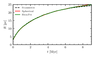
Figure 1: The location of the ionization front as a function of time for four sources each emitting $2.5\times 10^{48}\,\mathrm{s^{-1}}$ placed at the centre of a box filled with a uniform medium with a density of $100\,\mathrm{cm^{-3}}$ and a temperature of $10^{3}\,\mathrm{K}$. The simulations are carried out with a gas mass resolution of $20\,\mathrm{M_{\odot}}$ with our photoionization scheme operating in the commonly adopted ‘spherical’ mode ($N_{\mathrm{pix}}=1$) and our improved HealPix scheme ($N_{\mathrm{pix}}=12$). Both schemes accurately capture the evolution of a D-type expansion, as compared to results from the RT code comparison project Starbench (Bisbas et al. 2015).

In order to demonstrate the advantage of our new HealPix scheme in an idealized manner, we repeat the previous experiment but additionally place a dense clump of gas near the sources. This takes the form of a sphere of radius 10 pc centred 20 pc from the origin, comprised of gas with a density of $10^{4}\,\mathrm{cm^{-3}}$ in pressure equilibrium with the background medium. Fig. 2 shows the temperature of the gas in a slice through the centre of the box after 8 Myr. We also mark with a green circle the location of the ionization front predicted by Starbench in the absence of the dense clump. If the spherical scheme is used, when the ionizing front makes contact with the dense clump it cannot advance in any direction without first starting to ionize the dense gas. This is equivalent to photons that should be emitted in the opposite direction to the clump being erroneously redirected towards it. The result is that a significant portion of the clump has been ionized or otherwise disrupted by the expanding H ii region by 8 Myr. An arc of cold material is noticeable as the dense clump is peeled off around the necessarily spherical H ii region. Meanwhile, the expansion of the ionized region (which is co-spatial with the hottest gas in the slice shown) into the lower density medium has been curtailed relative to the case without the dense clump. There is significant flow of warm (but not photoionized) material in the opposite direction to the clump due to the large pressure gradient across the region (since both the $10^{2}$ and $10^{4}\,\mathrm{cm^{-3}}$ gas is heated to $10^{4}\,\mathrm{K}$ when photoionized).

Alternatively, when our novel HealPix scheme is used, the dense clump is barely disturbed as it can effectively only receive ionizing photons sent in its direction. Meanwhile, the ionization front in other directions is set independently in each angular pixel. The result is that away from the dense clump, the ionization front is close to the result predicted in the absence of the clump. The shadow cast by the clump is coarse, but our angular resolution is sufficient to meet our aims of mitigating the erroneous mass-biasing errors present in a traditional spherical approach.

Finally, for any scheme such as ours it must be determined how frequently to recalculate the extent of the H ii regions. If the recalculation is not occurring every time-step, then gas cells must be ‘locked’ as either flagged (and have the temperature floor imposed) or unflagged. In addition, it must be decided whether all sources will refresh together in a synchronised manner or in an asynchronous manner (i.e. after a certain delay time from when they were first switched on). The latter case has the advantage of minimizing the potential impact of ‘flickering’, whereby the geometry of two overlapping regions may alternate back and forth from calculation to calculation in a non-deterministic manner. As the refresh rate is likely to be much faster than the cooling time of the gas, this can lead to a greater quantity of gas effectively pinned to $10^{4}$ K than can physically be photoionized at once. An asynchronous scheme usually results in only one of the overlapping regions being recalculated at once, making the results more consistent. The disadvantage is that an asynchronous scheme also requires a more complicated method of locking source stars to the refresh rate of the host cells in order to avoid double counting if they drift into another cell. We have implemented both approaches. In practice, we find that refreshing every fine time-step (i.e. the finest time-step in the hierarchy) or with some fixed refresh rate, in either a synchronous or asynchronous fashion, gives identical results with no evidence of ‘flickering’. The exception to this is if the refresh rate is set to be too slow.

We find that for the test case above, the H ii region must be recalculated at least as frequently as every 0.1 Myr. Longer refresh rates than this lead to stalling of the D-type expansion and severe underestimation of size of the H ii region (see Appendix C). We also find that the results from our global galaxy simulations, presented below, converge as long as the recalculation occurs more frequently than approximately 0.1 Myr. Slower refresh rates gradually reduce the impact of the feedback channel. In practice, we find that the computational cost of our algorithm is so low, even in our full galaxy simulations, that we can afford to adopt the simplest solution and execute the full photoionization algorithm every fine time-step for all sources.

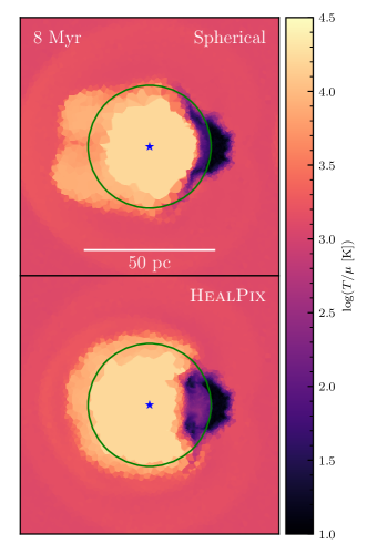
Figure 2: D-type expansion of an H ii region into a background of $100~{}\mathrm{cm^{-3}}$ gas as in Fig. 1, but this time with the addition of a clump of $10^{4}~{}\mathrm{cm^{-3}}$ gas offset from the centre. We show the temperature in a slice through the centre of the domain after 8 Myr. The green circle marks the expected radius of the ionization front predicted by Starbench in the absence of the dense clump. In the top panel, the common spherical method erroneously forces ionizing photons to be channelled towards the dense clump due to the mass-biasing effect. This disrupts the clump but also hinders the expansion of the photoionized region (co-spatial with the highest temperature gas) in the other directions. In the bottom panel, our new HealPix method only allows the clump to see photons emitted in angular pixels that it subtends. This leaves the clump relatively undisturbed and allows the expansion to continue unhindered in the other directions.

3.3.4 Supernovae

When a star in the mass range $8-35\,\mathrm{M_{\odot}}$ reaches the end of its life a SN event is triggered, resolved from the cell hosting the star particle. We employ the scheme for modelling individually time-resolved SNe as presented in Smith et al. (2018), operating in its mechanical feedback mode. The full details of the method can be found in that work, but we summarise the salient details here. When resolution permits, it is important to model SNe as individual events with the correct distribution in time, rather than continuously injecting a population averaged energy or injecting the total energy budget at one time. Failing to individually time-resolve SNe will result in an inability to capture the sensitivity to clustering and the interaction with other pre-SN feedback channels, as described in Section 1. Feedback quantities (i.e. ejecta mass, energy, momentum and metals) are distributed amongst the cell hosting the star particle and its immediate neighbours (i.e. those with which it shares a face), making use of a vector-weighting scheme to ensure an isotropic injection (which is otherwise non-trivial in a Lagrangian code, see also Hopkins et al. 2018a).

The mass and metallicity of the SN ejecta is determined as a function of progenitor mass from Chieffi & Limongi (2004). For particularly massive stars it is possible that the host star particle does not contain enough mass to meet this requirement. In this case, we return all of the mass that is available and delete the star particle. Due to the shape of the IMF, this is a sufficiently uncommon occurrence, resulting in an overall deficit in ejecta mass of $5.1\%$ given the star particle of $20\,\mathrm{M_{\odot}}$ used in this work. While this is not ideal, we believe that the magnitude is sufficiently small to have negligible impact on our results, particularly given uncertainties in the true ejecta properties of very massive stars. It would be of more concern if we were attempting to track individual metal species since this could potentially lead to a truncation of the products of the most massive stars. Similarly, for the purposes of this work we do not include Type Ia SNe which, while of interest for studying the chemical evolution of the galaxy, occur very rarely compared to core collapse SNe when star formation rates are relatively constant (as in this work).

All SNe inject $10^{51}$ ergs of energy. The host cell receives this in the form of thermal energy. Neighbour cells receive momentum directed radially away from the host cell. The mechanical feedback scheme corrects the magnitude of the injected momentum to account for missed $P\mathrm{d}V$ work if the adiabatic Sedov-Taylor phase of the SNR supernova remnant expansion has not been resolved (see e.g. Hopkins et al. 2014, 2018a; Kimm & Cen 2014; Martizzi et al. 2015 and for the details of our model see Smith et al. 2018). The calculations take place in the rest frame of the star particle before being transformed back to the simulation frame. For the fiducial mass resolution adopted in this work of $20~{}\mathrm{M_{\odot}}$, the study of Kim & Ostriker (2015a) suggests that SNRs begin to become only marginally resolved in gas denser than a few $\mathrm{cm^{-3}}$. This density is obviously significantly lower than the density of star forming regions. However, Smith et al. (2018) demonstrated that in practice this resolution is sufficient even without the mechanical feedback correction as most SNe occur in low density gas once the star forming cloud has been dispersed by the first SNe, with the mechanical feedback scheme converging with a more simple thermal dump of energy. Other studies have also shown that results are relatively insensitive to the exact SN feedback scheme adopted when the resolution is this high (see e.g. Hopkins et al. 2018b; Hu 2019; Wheeler et al. 2019). We have confirmed that using a simple thermal dump instead of mechanical feedback in this work provides very similar results.

4 Initial conditions and simulation details

We simulate idealized, isolated dwarf galaxies comprised of a disc of gas and pre-existing stars, and a dark matter halo. Initial conditions are generated using the code MakeNewDisk (Springel et al. 2005). We simulate three systems which we refer to as ‘fiducial’, ‘low-$\Sigma$’ and ‘high-$\Sigma$’. The fiducial system is derived from initial conditions developed for a code comparison project undertaken by the SMAUG collaboration (Hu et. al. 2021 in prep.) intended to be loosely representative of Wolf-Lundmark-Melotte (WLM). All systems have a total mass of $10^{10}\,\mathrm{M_{\odot}}$. In the fiducial system, the gas and stellar discs have masses of $6.825\times 10^{7}\,\mathrm{M_{\odot}}$ and $9.75\times 10^{6}\,\mathrm{M_{\odot}}$, respectively. The low-$\Sigma$ system has discs of half the mass while the heavy system has discs of twice the mass. The gas and stellar discs have density profiles that are exponential in radius, with a scale length of 1.1 kpc. The stellar disc has a Gaussian vertical density profile with a scale height of 0.7 kpc. The gas disc is initialised with an initial temperature of $10^{4}\,\mathrm{K}$ with its vertical structure set to achieve hydrostatic equilibrium. The gas has an initial metallicity of $0.1\,\mathrm{Z_{\odot}}$. The pre-existing stellar disc does not contribute to feedback. The remainder of the system is made up by the spherically symmetric dark matter halo, modelled with a Hernquist (1990) density profile chosen to provide a close match to an Navarro et al. (1997) density profile with a concentration parameter, $c$, of 15 and a spin parameter, $\lambda$, of 0.04. We do not include a CGM in this work. While this is not fully realistic, we wish to study the evolution of the disc without inflowing gas. The gas cells and star particles have a mass of $20\,\mathrm{M_{\odot}}$ (refinement/derefinement keeps the gas cells within a factor of 2 of this target) while the dark matter particles have a mass of $1640\,\mathrm{M_{\odot}}$. We use a gravitational softening length of 20 pc for dark matter particles and 1.75 pc for star particles (whether pre-existing or formed during the simulation). Gas cells have adaptive softening lengths down to a minimum of 1.75 pc.

After being generated by MakeNewDisk, the initial conditions undergo the background mesh adding and relaxation procedures described in Springel (2010). The final stage in preparing the initial conditions is to generate some initial level of turbulent support in order to avoid the rapid vertical collapse of the disc when the simulation is started. Without initial driving, this rapid collapse results in an extremely thin disc and a large starburst. In simulations with SN feedback, this leads to complete disruption of the centre of the disc and the removal of a large amount of material. If the simulation is run for long enough ($\sim 1$ Gyr), the disc eventually settles back into a stable equilibrium but by this time the properties of the disc (in particular surface density) has changed sufficiently to make comparison between different simulations impossible. We therefore initially pre-process our initial conditions by running them for 100 Myr with radiative cooling switched on, star formation switched off and turbulent driving provided by a modified version of our fiducial SN feedback scheme. We calculate a pseudo-star formation rate for all gas cells with a density greater than $0.1\,\mathrm{cm^{-3}}$ using a low efficiency of $\epsilon_{\mathrm{SF}}=0.002$. However, instead of sampling this rate to produce star particles, we instead sample this rate to trigger SNe assuming that 1 SN occurs for every $100\,\mathrm{M_{\odot}}$, injecting $10^{51}\,\mathrm{ergs}$ of thermal energy (but no ejecta). This preserves the large scale features of the initial conditions, but substantially reduces the unphysical transient phase at the beginning of the actual simulation. The choice of parameters for this driving (the density threshold and $\epsilon_{\mathrm{SF}}$) are chosen empirically; we use the same across all three sets of initial conditions for consistency, although in the case of the fiducial and high-$\Sigma$ systems the initial transient is not entirely eliminated.

We present simulations with various combinations of our three feedback channels, using the notation SN, PI and PE to refer to supernova feedback, photoionization and photoelectric heating, respectively. We use NoFB for runs without feedback. In simulations that do not include SN feedback (including NoFB runs) we still return mass and metals when a star in the range $8-35\,\mathrm{M_{\odot}}$ reaches the end of its life, distributing them using the scheme described above but without adding the $10^{51}\,\mathrm{ergs}$ of SN energy. This is to ensure the return of mass from stars to the ISM is consistent between all simulations. The colours used in figures remain completely consistent throughout this work for our fiducial feedback schemes (as first introduced in Fig. 6). For non-standard variations of our feedback schemes (Section 5.6 onwards), colours are necessarily reused from subsection to subsection. Table 1 contains a list of the 32 simulations explicitly presented in this work. Various other test runs that are mentioned in the text but that do not feature in any plots are not listed.

Table 1: A summary of the various simulations presented in this work for the convenience of the reader. The ‘Galaxy’ column denotes which of our three initial conditions was used. The ‘SN’, ‘PI’ and ‘PE’ columns indicate whether supernova feedback, photoionization and/or photoelectric heating were active, respectively. In the main text and in figure legends these are referred to as, for example, SN-PI-PE. Simulations use the fiducial parameters for our sub-grid models given in Section 3 with exceptions given in the ‘Non-fiducial parameters’ column. The ‘Section’ column gives the section (or appendix) where the simulation is first introduced. Note that this table only lists simulations that have results explicitly shown in this work, omitting other test runs that may be briefly referred to in the text.

Galaxy	SN	PI	PE	Non-fiducial parameters	Section
Fiducial	$\times$	$\times$	$\times$	-	5.1
Fiducial	$\checkmark$	$\times$	$\times$	-	5.1
Fiducial	$\times$	$\checkmark$	$\times$	-	5.1
Fiducial	$\times$	$\times$	$\checkmark$	-	5.1
Fiducial	$\checkmark$	$\times$	$\checkmark$	-	5.1
Fiducial	$\checkmark$	$\checkmark$	$\checkmark$	-	5.1
Fiducial	$\checkmark$	$\checkmark$	$\checkmark$	$N_{\mathrm{J,SF}}=160$, pressure floor at $N_{\mathrm{J,PF}}=80$	5.6
Fiducial	$\checkmark$	$\checkmark$	$\checkmark$	$\epsilon_{\mathrm{SF}}=100\%$	5.6
Fiducial	$\checkmark$	$\checkmark$	$\checkmark$	Additional SF threshold $n_{\mathrm{SF}}=10^{3}\,\mathrm{cm^{-3}}$	5.6
Fiducial	$\checkmark$	$\checkmark$	$\checkmark$	Additional SF threshold $n_{\mathrm{SF}}=10^{4}\,\mathrm{cm^{-3}}$	5.6
Fiducial	$\checkmark$	$\checkmark$	$\checkmark$	Additional SF threshold $n_{\mathrm{SF}}=10^{4}\,\mathrm{cm^{-3}}$, $\epsilon_{\mathrm{SF}}=100\%$	5.6
Low-$\Sigma$	$\times$	$\times$	$\times$	-	A
Low-$\Sigma$	$\checkmark$	$\times$	$\times$	-	A
Low-$\Sigma$	$\times$	$\checkmark$	$\times$	-	A
Low-$\Sigma$	$\times$	$\times$	$\checkmark$	-	A
Low-$\Sigma$	$\checkmark$	$\times$	$\checkmark$	-	A
Low-$\Sigma$	$\checkmark$	$\checkmark$	$\checkmark$	-	A
High-$\Sigma$	$\times$	$\times$	$\times$	-	A
High-$\Sigma$	$\checkmark$	$\times$	$\times$	-	A
High-$\Sigma$	$\times$	$\checkmark$	$\times$	-	A
High-$\Sigma$	$\times$	$\times$	$\checkmark$	-	A
High-$\Sigma$	$\checkmark$	$\times$	$\checkmark$	-	A
High-$\Sigma$	$\checkmark$	$\checkmark$	$\checkmark$	-	A
Fiducial	$\times$	$\times$	$\checkmark$	No FUV attenuation	B
Fiducial	$\times$	$\times$	$\checkmark$	Linear DGR-metallicity relationship	B
Fiducial	$\times$	$\times$	$\checkmark$	No FUV attenuation, linear DGR-metallicity relationship	B
Fiducial	$\times$	$\times$	$\checkmark$	No FUV attenuation, linear DGR-metallicity relationship, fixed $\epsilon_{\mathrm{PE}}=0.041$	B
Fiducial	$\checkmark$	$\checkmark$	$\checkmark$	$r_{\mathrm{ion,max}}=50\,\mathrm{pc}$	C
Fiducial	$\checkmark$	$\checkmark$	$\checkmark$	$r_{\mathrm{ion,max}}=20\,\mathrm{pc}$	C
Fiducial	$\checkmark$	$\checkmark$	$\checkmark$	Photoionization limited to host cell	C
Fiducial	$\times$	$\checkmark$	$\times$	Long-range photoionization scheme	D
Fiducial	$\checkmark$	$\checkmark$	$\checkmark$	Long-range photoionization scheme	D

5 Results

We now present the results of our simulations. Sections 5.1-5.5 are concerned with our main six simulations (NoFB, SN, PI, PE, SN-PE and SN-PI-PE) in our fiducial galaxy. They show galaxy morphologies (Section 5.1), gas phase diagrams (Section 5.2), global star formation rates (Section 5.3), outflow rates (Section 5.4), and details of the local environment and clustering properties of SNe (Section 5.5). Section 5.6 examines the dependence of results on the SF prescription.

5.1 Morphologies

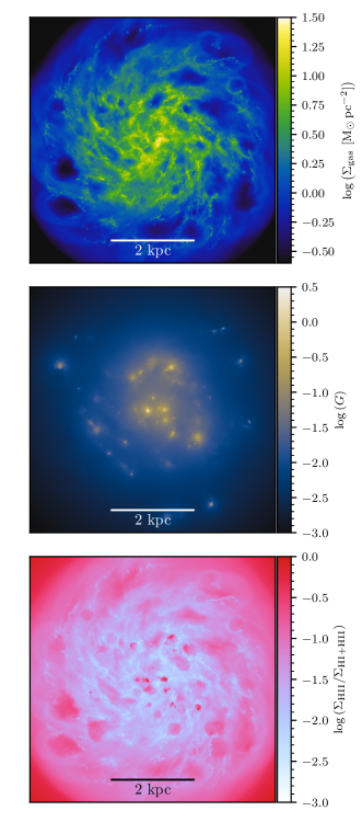
Figure 3: Face-on projections of the fiducial galaxy after 1 Gyr with all stellar feedback channels switched on (SN-PI-PE). Top: gas column density. Middle: mass-weighted FUV energy density normalised to the Habing (1968) field. Bottom: Ratio of the surface densities of ionized hydrogen to total hydrogen (effectively a projected ionization fraction). The ionized regions largely trace diffuse gas, but several concentrated patches of completely ionized material are visible. These are H ii regions around massive stars. The distribution of peaks in the FUV energy density and H ii regions are highly clustered, corresponding to the distribution of (relatively short lived) massive stars.

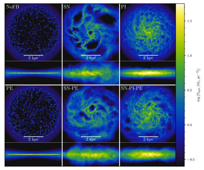
Figure 4: Face-on and edge-on projections of the gas distribution after 1 Gyr for the fiducial galaxy with various combinations of the available feedback channels. Without feedback (NoFB) or with only photoelectric heating (PE) the disc is very thin and highly fragmented, with much of the initial gas having been converted into stars. With SNe, either alone (SN) or in combination with photoelectric heating (SN-PE), the disc contains larger, more diffuse structures. Holes in the disc are apparent, caused by SN superbubbles. The vertical structure is thicker and more complex. With photoionization alone (PI), fragmentation is significantly reduced relative to the no feedback case, but dense clumps remain. A thicker, more diffuse disc is present. With all feedback switched on (SN-PI-PE), the morphology lies qualitatively between the SN and PI cases.

Fig. 3 shows face-on visualisations of the fiducial galaxy after 1 Gyr with all stellar feedback channels switched on (SN-PI-PE). The top panel shows the gas column density. The gas has a complex morphology, comprised of clumps and filaments of dense gas embedded in more diffuse material. The largest complexes of dense gas can be found in the centre of the galaxy, as is to be expected given the initial exponential radial surface density profile, but more isolated regions of dense, star-forming gas also exist in the outskirts of the disc.

The middle panel of Fig. 3 shows the (mass-weighted) projected FUV energy density, normalised to the Habing (1968) field. Significant spatial variation is in evidence, with regions of relatively high FUV energy density tracing recent star formation. In a broad sense, the spatially averaged emission falls off with radius as the combination of the decline in the SFR surface density and the inverse-square law. However, the distribution is highly clustered and dominated by regions of high energy density surrounding massive stars. This clustering means that the distribution would not be well modelled by, for example, a simple radial profile. Some degree of correlation of the bright patches with the morphology of the gas is apparent by visual inspection, although there are also regions of high energy density in more diffuse gas, particularly in the outskirts of the disc where the gas surface density is lower. These indicate the presence of massive stars that are no longer co-spatial with star-forming gas, typically because it been dispersed by feedback.

The bottom panel of Fig. 3 shows the ratio of the surface density of ionized hydrogen to total hydrogen (i.e. a form of projected ionization fraction). Generally, comparing to the top panel of the figure, it can be seen that the neutral regions trace the dense gas while more diffuse regions are ionized, as would be expected. A temperature map (not shown) shows similar features. However, a few regions of near unity ionization fraction are embedded in or are close to dense filaments. These are H ii regions created by our sub-grid scheme. They correlate with some of the peaks in the FUV energy density distribution because they are created by the same massive stars. Other H ii regions are not apparent from this figure as they are too small to be distinguished.

Fig. 4 shows face-on and edge-on projections of the gas distribution after 1 Gyr for six realisations of the fiducial galaxy with various combinations of the available feedback channels. Without feedback (NoFB), a very thin disc forms with limited vertical sub-structure. The disc is extremely fragmented, its morphology being dominated by small, dense clumps and voids. A significant fraction of the initial gas has been converted into stars (more details follow in later sections) so the overall gas surface density is lower than some of the other simulations. The simulation with only photoelectric heating switched on (PE) is very similar to the no feedback case. There is slightly more gas left in the centre of the disc, but the difference is very marginal.

The simulations with SNe only (SN) and SNe with photoelectric heating (SN-PE) have similar morphologies. The dense clumps seen in the no feedback case are absent. Instead the morphology is dominated by relatively large (typically several hundreds of parsecs) structures. On close inspection, the large structures do contain denser substructures composed of filaments and clumps. This is where star formation occurs. Multiple large holes blown by SNe are present. The vertical structure of the disc is significantly different from the no feedback case, with a much thicker distribution of gas. The relatively diffuse material is spread reasonably evenly about the disc mid-plane. However, the denser structures described previously can be seen to have complex morphologies when viewed edge on, with clumps existing several hundred parsecs above and below the mid-plane.

The simulation with photoionization feedback alone switched on (PI) produces large complexes of dense gas at the centre of the disc, but avoids the extreme fragmentation that occurs in the no feedback case. The disc still contains a multitude of small, dense clumps of gas, either embedded in the central complexes or in the more diffuse gas at the edges of the disc. Seen edge-on, the morphology is comprised of a thin disc structure at the mid-plane and a more extended distribution of lower density gas. The thin disc is qualitatively similar to that seen in the no feedback simulation, although marginally thicker. The central complexes of gas apparent in the face-on view manifest themselves as a slight bulge of dense material. Despite lacking SNe to expel gas out of the disc, it seems that the photoionization feedback is still able to prevent all the gas settling into the thin disc. This is because the H ii regions impart momentum to the ISM as they expand.

The face-on projection of the simulation with all feedback switched on was also shown in Fig. 3, but it is instructive to compare it to the other simulations. The morphology is qualitatively similar to the simulation with photoionization only, with some differences. The large complexes of dense gas seen in the photoionization only simulation persist with the addition of SNe, although not to the same degree. The amount of fragmentation has been reduced, but a more clumpy morphology is present relative to the SN only simulation. The disc morphology is not as chaotic as the other SNe simulation. There is a lack of large SNe driven holes in the central regions of the disc, although smaller holes are apparent at various points through the course of the simulation and larger holes form at the outer regions of the disc. The disc mid-plane is still relatively well defined but the disc is marginally thicker than the photoionization only case.

5.2 Gas phase diagrams

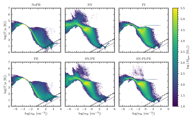
Figure 5: Phase diagrams at 1 Gyr for the fiducial galaxy for simulations with various combinations of feedback. The dashed line indicates the star formation threshold at $M_{\mathrm{J}}=8m_{\mathrm{cell}}$ while the dotted line indicates $M_{\mathrm{J}}=m_{\mathrm{cell}}$. Relatively large quantities of hot, low density gas (in SN bubbles and outflows) are only apparent in runs SN and SN-PE. Adding photoionization feedback (SN-PI-PE) significantly reduces gas in this phase, while adding a region of dense $10^{4}$ K gas in H ii regions. The slight ‘tick’ shape apparent in the gas distribution of gas at high densities is related to the self-shielding prescription and non-equilibrium chemistry; we have confirmed with simulations without UV heating and equilibrium chemistry that this artefact does not impact our results.

Fig. 5 shows phase diagrams for the fiducial galaxy simulations at 1 Gyr. All simulations have gas at a wide range of densities. In particular, all simulations have a small population of cold, dense gas that is capable of forming stars. The exact shape of the equilibrium curve in this region shows a slight ‘bump’ and an upwards ‘tick’ towards the highest density. This artefact is caused by the interaction of the non-equilibrium cooling with the UV background and self-shielding prescription at high densities. We have confirmed by altering the scheme (removing UV background heating, using equilibrium chemistry etc.) that this artefact has no impact on the dynamics of the gas and star formation. For all simulations, the majority of gas is warm ($\sim 10^{4}$ K) and diffuse ($n<0.1\,\mathrm{cm^{-3}}$).

NoFB and PE give almost identical distributions of gas in phase space by 1 Gyr, with only minor evidence of photoelectric heating at high density, if any. After 1 Gyr the gas has been substantially depleted in these simulations by a large amount of star formation relative to the others. Most gas lies in a much narrower distribution at densities above $0.01\,\mathrm{cm^{-3}}$ relative to the other four simulations which have a much wider range of temperatures. SN and SN-PE show substantial amounts of hot ($T>10^{4}$ K) gas. This can be seen at intermediate densities ($10^{-4}-1\,\mathrm{cm^{-3}}$) as SN bubbles expand in the disc and in a reservoir of more diffuse gas as the the bubbles break out and form a CGM via outflows. The simulation with photoionization alone (PI) does not produce this hot gas phase, but high density ($1-10^{4}\,\mathrm{cm^{-3}}$) photoionized gas in H ii regions appears as a narrow, isothermal line. Note that this population of gas is distinct from the warm, neutral gas at a similar temperature because we choose to plot $T/\mu$ to emphasize the two components. When all feedback channels are combined (SN-PI-PE), the phase diagram is very similar to the photoionization only simulation. A small population of hot gas is apparent, corresponding to the rare SN bubbles apparent in Fig. 4 but the reservoir of hot, outflow/CGM gas apparent in the other runs that include SN feedback does not exist.

5.3 Star formation rates

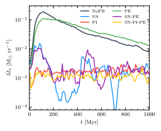
Figure 6: The star formation rate (SFR) as a function of time for the fiducial galaxy simulations, averaged over 10 Myr. Without any feedback (NoFB), the SFR climbs until it is limited by the available gas reservoir, gradually decreasing as this is exhausted. Adding photoelectric heating (PE) has a negligible impact, reducing SFR marginally (which results in the gas reservoir being depleted slightly slower). Adding either SN feedback or photoionization (PI) leads to a reduction in SFR by a factor of 10-100 on average. SN has a more bursty SFR than PI. Combining all the feedback channels (SN-PI-PE) results in a slight additional suppression, but this is small compared to the initial suppression caused by adding one effective feedback channel. Fig. 15 in Appendix A shows equivalent plots for the low-$\Sigma$ and high-$\Sigma$ galaxies.

Fig. 6 shows the star formation rates (SFR) as a function of time for the simulations of the fiducial galaxy, averaged over 10 Myr. Note that because the disc has already been pre-processed with cooling and initial turbulent driving for 100 Myr, the SFR is non-zero at the start of the simulation, although star formation was switched off during the pre-processing phase. Without any feedback, the SFR rises rapidly over the first 100 Myr as the disc collapses vertically and fragments, reaching a peak of approximately $0.2\,\mathrm{M_{\odot}\,yr^{-1}}$. The SFR is limited only by the available reservoir of gas and the rate at which it can cool and collapse into dense clumps. Over the remaining 900 Myr, the SFR smoothly declines to $\sim 0.01\,\mathrm{M_{\odot}\,yr^{-1}}$ as the gas supply is exhausted. When photoelectric heating is added as the sole form of feedback, the results are similar. The feedback is able to produce a slight suppression of star formation, reducing the peak SFR to approximately a factor of 2. Despite this, the galaxy is still experiencing runaway star formation with the feedback unable to halt the overall fragmentation of the disc (as seen in Fig. 4). The slight reduction of the SFR does mean that the gas reservoir is consumed a little slower than the no feedback case, so the peak SFR is maintained for longer. The result is that from $\sim 300\,\mathrm{Myr}$ onwards, the SFR is marginally higher than the run without feedback. This is entirely a product of our idealized initial conditions; in a full cosmological setting some amount of gas would be accreting into the system.

When SN feedback is included, the SFR is suppressed by approximately 2 orders of magnitude (at late times, the difference is only a factor of 10, but this is due to gas depletion in the the no feedback case). For the first 10s of Myr, the SFR is similar to the no feedback case because there is a delay between star formation and SNe occurring. Then, as the first SNe start exploding, a burst of feedback drops the SFR down by almost two orders of magnitude. The SFR rises again, but is subsequently regulated by feedback. After this initial transient phase (which is substantially reduced by our pre-processing method), the SFR settles into a more steady state, although it still proceeds in a bursty manner. From 500 Myr onwards, the SFR averages $1.84\times 10^{-3}\,\mathrm{M_{\odot}\,yr^{-1}}$. Adding photoelectric heating to the SN feedback (SN-PE) produces very similar results. The initial suppression of star formation after the first burst of feedback is not quite as deep, but behaviour thereafter is similar, averaging $2.26\times 10^{-3}\,\mathrm{M_{\odot}\,yr^{-1}}$ after 500 Myr. The simulation of the fiducial galaxy with photoionization as the sole feedback channel (PI) starts with an initially lower SFR than SNe simulations since this form of feedback starts operating as soon as a massive enough star is formed. After a 50 Myr transient phase, a relatively constant SFR is established, without bursts such as those seen in the simulations with SN feedback (with or without photoelectric heating). The average from 500 Myr is $1.77\times 10^{-3}\,\mathrm{M_{\odot}\,yr^{-1}}$. It is therefore apparent that the SN feedback or the photoionization are both capable of regulating the SFR to approximately the same average value. The degree of burstiness, on the other hand, is a real difference in behaviour between the two feedback channels.

Finally, we consider the fiducial galaxy with all feedback channels (SN-PI-PE) switched on. The SFR initially follows the same evolution as the photoionization only run, which is expected. Then, once SN feedback begins to occur the SFR is suppressed marginally relative to the PI simulation. Like the PI simulation, the SFR can be seen to be significantly smoother than the SN or SN-PE simulations. The average SFR after 500 Myr is $1.16\times 10^{-3}\,\mathrm{M_{\odot}\,yr^{-1}}$. Thus combining all the feedback results in an average SFR that is $\sim 60\%$ of the simulations with only SN or photoionization feedback. However, it is important to bear in mind that it is difficult to draw firm conclusions based on such minor differences given the sensitivity to choices of numerical methods, parameters and even noise arising from non-deterministic computations (see e.g. Keller et al. 2019). However, what is apparent is that including one of either SN or photoionization feedback results in a similar, significant reduction in SFR relative to no feedback (or photoelectric heating only) but that adding the other feedback channel results in insignificant additional suppression of SFR in a relative sense. However, photoionization produces significantly less bursty regulation of star formation than SN feedback and this effect persists even when the two are combined. We show in Appendix A that these qualitative trends persist in our low-$\Sigma$ and high-$\Sigma$ galaxies.

5.4 Outflows

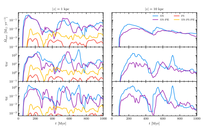
Figure 7: Outflow rates for the fiducial galaxy across thin slabs parallel to the disc at 1 kpc and 10 kpc. Mass and energy loadings are averaged over 10 Myr. Photoelectric heating does not drive outflows above the background no feedback rate (see text for details) so is not included. With SN feedback (with or without photoelectric heating), very efficient outflows are generated with high mass loadings. The addition of photoionization feedback substantially curtails outflows. Fig. 16 in Appendix A shows equivalent plots for the low-$\Sigma$ and high-$\Sigma$ galaxies.

We now examine the galactic outflow rates. We calculate the instantaneous mass outflow rate through a slab of thickness $\Delta z$ parallel to the disc plane as:

$$\dot{M}_{\mathrm{out}}=\frac{\sum_{i}\left(m_{i}v_{\mathrm{out},i}\right)}{\Delta z},$$ (10)

where the sum as carried out over all cells within the slab that have a positive outflow velocity perpendicular to the disc plane. We make these measurements for a slab at a distance of 1 kpc from the disc mid-plane with $\Delta z=0.1\,\mathrm{kpc}$ and another at a height of 10 kpc with $\Delta z=0.2\,\mathrm{kpc}$. Additionally, for the measurement at 1 kpc we include only gas within a cylindrical radius of 4 kpc in order to avoid erroneous contributions from gas motions in the flared disc at large radii. Due to the idealized initial conditions and pre-simulation turbulent driving, very weak outflows ($\lesssim 10^{-3}\,\mathrm{\mathrm{M_{\odot}}\,yr^{-1}}$ through 1 kpc) are present in the no feedback run. As these have a non-physical origin (and to avoid presenting misleading loading factors by associating these outflows with star formation) we subtract the measured NoFB rates from the total measured in all simulations.

In addition to considering the absolute mass outflow rates, it is often useful to scale them by the global SFR rate. We therefore obtain the mass loading factor:

$$\eta_{M}=\frac{\dot{M}_{\mathrm{out}}}{\dot{M}_{\star}}.$$ (11)

Since the main use of the mass loading factor is to relate the outflow rates to the star formation that caused it, the most rigorous way to make this measurement would be to compare the outflow rates to the global SFR some time in the past when the outflows were launched. However, there is obviously no single wind travel time unless a single outflow velocity is present in all cases. We therefore take a much cruder but simpler approach and compare the instantaneous mass outflow rate to the global SFR averaged over the previous 10 Myr. When the SFR is relatively constant this is a very good approximation, however if the SFR is bursty (e.g. simulations SN and SN-PE) this will obviously induce larger amplitude oscillations in the mass loading factor. However, with this caveat, we find that this simple approach serves our purpose here.

We also measure the energy outflow rates through these slabs as:

$$\dot{E}_{\mathrm{out}}=\frac{\sum_{i}\left[m_{i}v_{\mathrm{out},i}\left(\frac{1}{2}v_{i}^{2}+\frac{c_{\mathrm{s,i}}^{2}}{\gamma-1}\right)\right]}{\Delta z},$$ (12)

where $c_{\mathrm{s}}$ is the sound speed. Again, we subtract the (very weak) rates from the NoFB simulation. In an analogous fashion to the mass loading factor, we can define an energy loading factor,

$$\eta_{E}=\frac{\dot{E}_{\mathrm{out}}}{\dot{M}_{\star}u_{\star}},$$ (13)

where $u_{\star}$ is some reference feedback energy per stellar mass formed. We use $u_{\star}=4.89\times 10^{5}\,\mathrm{km^{2}\,s^{-2}}$, corresponding to 1 SN with an energy of $10^{51}$ ergs for every 102.6 $\mathrm{M_{\odot}}$ of stars formed (consistent with our IMF and SN progenitor mass range). Note that this value is not completely consistent with the actual amount of feedback energy available in our simulations because it does not include contributions from the radiative feedback. Likewise, it is obviously not directly applicable to the runs that do not include SNe. However, it is a convenient scaling that makes it easier to compare simulations in this work, as well as to other works.

Fig. 7 shows the absolute mass outflow rates, the mass loading factor and the energy loading factor for realisations of the fiducial galaxy, measured at 1 kpc and 10 kpc as described above. Including photoelectric heating does not drive outflows above the weak NoFB rates that arise from the settling of the initial conditions, so this run is not shown. The simulations with SN feedback only or with the addition of photoelectric heating do drive significant outflows, with similar rates. The large bursts of star formation within the first 500 Myr (as seen in Fig. 6) give rise to corresponding bursts of outflow, peaking at over 0.1 $\mathrm{M_{\odot}yr^{-1}}$ through 1 kpc. Even with the more settled SFR in the latter half of the simulation, outflow rates remain high with mass loading factors in excess of 10. The energy loadings are similarly high, generally in excess of 0.01 with peaks of up to 0.1 (though the susceptibility of amplification of peaks and troughs in the loading factors in the presence of a bursty SFR must be borne in mind, as described above). A large proportion of these outflows reach a height of 10 kpc, with rates in the last 500 Myr between $10^{-3}-10^{-2}\,\mathrm{M_{\odot}\,yr^{-1}}$, corresponding average mass loadings between 1-10. The simulation with only photoionization feedback produces a weak outflow through 1 kpc. This is a very small, low altitude fountain flow as the expanding H ii regions near the centre of the disc impart momentum to the gas. This has a significantly sub-unity mass loading.

Interestingly, when photoionization feedback is added to SN feedback, outflow rates are significantly reduced. The simulation with all feedback turned on (SN-PI-PE) does have an outflow at all times through 1 kpc, between $\sim 10^{-3}-10^{-2}\,\mathrm{M_{\odot}\,yr^{-1}}$. This corresponds to mass loadings between $\sim$1-10 and energy loadings between $\sim 10^{-3}-10^{-2}$. However, while this is larger than the small fountain produced by the PI simulation, it is still over an order of magnitude lower than the SN simulations without photoionization. It is also significantly less bursty. None of this outflow reaches 10 kpc. Given that this simulation has very similar average SFR to the SN and SN-PE simulations, it is clear that the addition of our short range photoionization scheme suppresses the generation of large outflows by some mechanism. The suppression also occurs in our low-$\Sigma$ and high-$\Sigma$ galaxies (see Appendix A). We shall explore the cause of this behaviour in the following section.

5.5 The local environment of SNe and their clustering

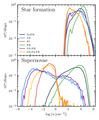
Figure 8: PDFs of the densities of the birth site of stars (top) and SN locations (bottom) for the fiducial galaxy. Note that in runs without SN feedback, we still return mass when a star in the SN progenitor mass range reaches the end of its life, but do not include additional energy. The first 200 Myr are not included.

As mentioned in the previous section, due to similar average SFRs, simulations SN, SN-PE and SN-PI-PE experience essentially the same number of SNe after the initial transient phase (within a factor of 1.7 for those occurring after 200 Myr). However, the outflow properties generated by SN feedback are substantially different. The cause must therefore be related to the local environment of SN events. A point frequently made when considering the efficiency of SN feedback is that it is at its most effective when SNe occur in low density environments. This is because as the ambient density increases, radiative losses become more important, reducing the work done on the ISM during the adiabatic Sedov-Taylor phase of the blast wave, leading to a smaller fraction of the SN energy retained in the resulting hot bubble and requiring a greater mass to be swept up before breakout is achieved, lowering the velocity of the material.

In Fig. 8 we show the distributions of the ambient density where stars are born and where SNe occur for the six realisations of our fiducial galaxy. Simulations without SN feedback are included as we still record where SN events would occur if the feedback was switched on and return the ejecta mass, as described in Section 3. The first 200 Myr while the disc is settling are not included. The range of stellar birth densities spanned is relatively similar across all simulations. The onset of star formation occurs between $\sim 20-100\,\mathrm{cm^{-3}}$ as the Jeans mass of the cell drops below our adopted threshold of $8m_{\mathrm{cell}}$. This can also be seen in Fig. 5 where a line indicating this threshold value intersects the distributions of gas in phase space. The simulations without feedback (NoFB) or with photoelectric heating only (PE) have a peak in their birth density distribution near $10^{4}\,\mathrm{cm^{-3}}$ as gas collapses beyond the threshold. The distribution then drops steeply with a maximum density reached of $10^{6}\,\mathrm{cm^{-3}}$ for a very rare number of star particles. Differences between NoFB and PE are driven by the effective time offset in their evolution as photoelectric heating briefly impedes disc fragmentation, as can be seen with reference to the SFRs in Fig. 6. With the inclusion of SN feedback, the distribution covers the same range but the peak is broadened, with an essentially flat PDF between $10^{2}-10^{4}\,\mathrm{cm^{-3}}$. This is because this feedback mechanism broadens the density PDF of star forming regions, reducing the formation of extremely dense clumps. This is also apparent from the projections in Fig. 4. The addition of photoelectric heating to SN feedback (SN-PE) does not make an appreciable difference. When photoionization feedback is used, either on its own (PI) or with SNe and photoelectric heating (SN-PI-PE), the distribution is skewed towards lower densities. The peak is at $100\,\mathrm{cm^{-3}}$, with a tail to higher densities, indicating that most star formation occurs at the threshold with a smaller amount of gas collapsing to higher densities relative to the other simulations.

The PDF of the local gas density where SN progenitors end their lives is similar to the PDF of birth densities for the NoFB and PE simulations, due to the lack of effective feedback dispersing star forming clouds. There is a tail to lower densities, demonstrating that some SN progenitors end up in lower density gas, with a minimum of about $10^{-2}~{}\mathrm{cm^{-3}}$. This is caused both by rapid gas depletion due to unrestricted star formation in the dense star forming clumps and by star particles wandering out of their extremely compact birth clouds. For simulations SN and SN-PE, the PDFs are very broad, spanning $\sim 10^{-5}-10^{5}~{}\mathrm{cm^{-3}}$. A slight hint of a double peak is evident. The SNe occurring at high densities originate from stars still inside their natal clouds, the high density end of the PDF overlapping with the equivalent PDF for birth density. These SNe will be inefficient due to radiative losses but are still able to disperse the cloud. This means that subsequent SNe, formed prior to the cloud’s dispersal but that have not yet reached the end of their lifetimes, will explode in the resulting lower density environment. This gives rise to SN superbubbles as successive SNe occur in the remnants of their predecessors, giving rise to the low density tail of the PDF. It is these SNe that are able to inflate the superbubble until it breaks out of the disc, resulting in strong outflows from the galaxy.

When photoionization is included (either PI or SN-PI-PE), there is essentially no overlap between the density PDFs for the birth sites and the SN sites. Very few SN progenitors end their lives in gas more dense than $1\,\mathrm{cm^{-3}}$. This indicates that our local photoionization prescription is able to efficiently disperse star forming gas around newly formed star particles prior to the first SNe occurring. Therefore, for simulation SN-PI-PE, all SNe occur in low density gas where they should, in principle, be at their most effective. Indeed, it is this phenomenon that is often invoked to suggest that efficient pre-SN feedback should enhance the impact of SNe. However, as we have seen in Section 5.4, this simulation has extremely curtailed outflows relative to simulations that are unable to clear this dense gas. We can also see from Fig. 8 that the PDF of SN densities does not extend into the low density regime as far as the simulations without photoionization feedback, with a peak at $\sim 0.1~{}\mathrm{cm^{-3}}$ and a low density tail that doesn’t extend far beyond the PI case, reaching $\sim 10^{-4}~{}\mathrm{cm^{-3}}$. As we have previously mentioned, the total number of SNe is almost identical in SN and SN-PI-PE, and in both cases SNe are occurring at relatively low densities (all of them for SN-PI-PE). Yet, simulation SN-PI-PE struggles to produce superbubbles and strong outflows.

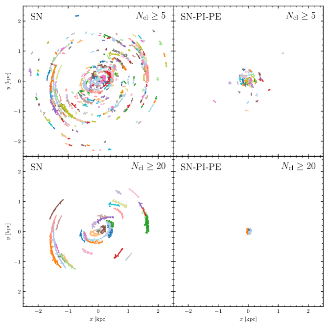
Figure 9: For the fiducial galaxy and runs SN (left) and SN-PI-PE (right), we plot the positions of SNe colour coded by cluster membership. Cluster membership is determined with a FoF algorithm with a linking length of 50 pc and a linking time of 4 Myr. These values do not represent a unique choice but were tuned to mitigate the opposing issues of over- and under-linking clusters as much as possible. Linking is carried out in the box rest frame, thus clusters trace out arcs as they orbit the galaxy. The top panels show SNe that occur in clusters larger than 5 SNe, the bottom panels show SNe that occur in clusters larger than 20 SNe. SNe that occur in the first 200 Myr are omitted. The addition of photoionization feedback results in a significant reduction in the number and size of clusters and restricts them to the centre of the galaxy.

It is therefore clear that the ability of SNe to drive outflows does not hinge solely on the total number of SNe events or the immediate local environment of individual SNe. Instead, we must examine the clustering properties of the SNe both in space and time. There are several metrics that could be used to quantify the relative degree of spatial clustering, for example a two-point correlation function of the locations of star particles (see e.g. Martizzi 2020; Keller & Kruijssen 2020). However, in this work, we choose to measure the relative clustering of the actual SN events themselves, since this is a more direct measure of SN clustering and takes the variations in the lifetimes of the progenitors into account. This necessarily involves associating SN events together in time as well as space. One could calculate the two-point correlation function in 4 dimensions (space and time) or alternatively make repeated 3 dimensional measurements with some window in time. However, we take a simpler approach and instead perform a ‘Friends of Friends’ (FoF) analysis of the SN events in 4 dimensions using both a linking length, $l_{\mathrm{link}}$, and a linking time, $t_{\mathrm{link}}$.

We record the spatial coordinates and time of every SN in the simulation. We choose a SN that has yet to be assigned to a cluster and search for any other SNe that occurred within a spatial separation of $l_{\mathrm{link}}$ and a time separation of $t_{\mathrm{link}}$ (before or after). Note that we perform this analysis in the simulation rest frame and do not attempt to correct for the bulk motion of the cluster of SNe progenitors in their galactic orbits which would add additional complexity to the analysis. Instead, we simply choose a suitable combination of $l_{\mathrm{link}}$ and $t_{\mathrm{link}}$ such that the effect of the bulk motion is not important. In addition to measuring the clustering of SN events, we also apply the same analysis to the clustering of SN progenitors at their birth.

The choice of $l_{\mathrm{link}}$ and $t_{\mathrm{link}}$ could in principle be determined a priori from some analytic estimate of relevant scales. However, in practice, we find that tuning the values by hand in order to minimize both over- and under-linking as apparent from visual inspection is sufficient. Note that this means our choice and the resulting cluster catalogue are by no means unique, but as will become apparent, the relative difference in clustering between our various simulations is of a significant enough magnitude to render this subjectivity negligible. We therefore adopt $l_{\mathrm{link}}=50\,\mathrm{pc}$ and $t_{\mathrm{link}}=4\,\mathrm{Myr}$.

In Fig. 9 we plot the locations of SNe associated with clusters, with points of the same colour indicating cluster membership. We plot SNe that occur after 200 Myr (the first burst of star formation as the disc settles in simulation SN generates an atypically large cluster), effectively projecting along the time axis, for simulations SN and SN-PI-PE. The top panels of the figure plot all SNe that are associated with a cluster of 5 or more SNe, while the bottom panels restrict the plotted SNe to those belonging to clusters with 20 or more SNe. The clusters trace out arcs in the rest frame of the simulation domain as they move in their orbits. It can be seen by visual inspection that some clusters lie close to each other along similar orbits but are not considered associated with each other (particularly for simulation SN), possibly indicating under-linking. Similarly, there are a few examples of clusters that trace out more complex shapes than a simple arc, indicating over-linking. As described above, there is no perfect choice for $l_{\mathrm{link}}$ and $t_{\mathrm{link}}$, with additional criteria for cluster membership being required if a cleaner analysis is required. Nonetheless, it should be clear that these details are relatively insignificant compared to the differences found between simulation SN and SN-PI-PE. With SN feedback only, a large number of clusters are present within 2 kpc of the galactic centre. By contrast, with the inclusion of the photoionization feedback it is clear that both the number and spatial extent of clusters are severely restricted. There are significantly fewer clusters of 5 or more SNe and almost all are within 1 kpc of the centre. There are only 3 clusters with 20 SNe or more and they are located at the very centre of the galaxy.

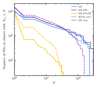
Figure 10: The number of SNe progenitors born (dashed line) or exploding (solid line) in clusters greater than some number, $N$, for simulations with SN feedback only (SN), the inclusion of photoelectric heating (PE) and the additional inclusion of photoionization feedback (SN-PI-PE). The first 200 Myr are not included in order to avoid the initial transient phase. Despite having a similar total number of SNe, without photoionization feedback SNe are considerably more clustered. The clustering of SNe is directly related to the clustering of the birth sites of their progenitors.

To enable a more quantitative comparison, in Fig. 10 we plot the total number of SNe exploding in clusters with more members than some number, $N$, for simulations SN, SN-PE and SN-PI-PE. We also plot the same metric for the clustering of SN progenitors at birth. As mentioned previously, it can be seen that the total number of SNe is very similar in all three simulations. However, it is clear that without photoionization SNe are more likely to be found in much larger clusters than when photoionization is included. Approximately half of all SNe occur in clusters with 4 or more members for simulation SN, but for SN-PI-PE that drops to $~{}7\%$. Again, $30\%$ of SNe occur in clusters of 10 or more with SN feedback alone but in the full feedback simulation that is true for only $3\%$. The largest cluster in SN-PI-PE is comprised of 34 SNe, compared to 229 for simulation SN. SN has 13 clusters with more than 50 SNe and 6 with more than 100. Similar results are found for SN-PE. The quantitative results depend on the exact values of $l_{\mathrm{link}}$ and $t_{\mathrm{link}}$ adopted but the qualitative trend remains for all reasonable choices.

By comparing the distribution of cluster membership of the SN progenitors at birth to the clustering of the eventual SNe, it is apparent that the reduction in the clustering of SNe is set at the point of star formation. In other words, for all 3 simulations shown the degree of clustering at birth is similar to that at the point of SN explosions. Clustering can be decreased from birth to death as SNe wander apart from each other over time but it can also be increased if separate clusters come together, particularly in the centre of the galaxy (as occurs for simulations SN and SN-PE). The relative level of clustering is also influenced by the difference in the spread of formation times within the cluster and the spread of stellar lifetimes drawn from the IMF. Some degree of noise also likely plays a role. Nonetheless, the level of clustering is more or less preserved from formation to eventual SNe events for these simulations.

Therefore, the difference in clustering properties of SNe between simulations with and without photoionization feedback is driven by the impact that the feedback has on the way in which clusters of stars assemble. In the case with SNe alone, a star produces no feedback until it reaches the end of its lifetime (and only if it is a SN progenitor). This means that star forming clouds are undisturbed for at least 6 Myr (the lifetime of a 35 $\mathrm{M_{\odot}}$ star, the largest SN progenitor mass we consider) after the onset of star formation, but more likely longer (since lower mass stars are more probable). This allows further star formation to proceed in the cloud over this time period, growing the cluster. Furthermore, as the cloud collapses, its SFR increases as the gas reaches higher densities, resulting in a higher effective star formation efficiency. As a consequence, by the time the first SN occurs there has been sufficient opportunity to build up a substantial cluster of stars. The first few SNe are able to begin dispersing the cloud. This quenches star formation, resulting in no more SN progenitors being formed. However, by this point, many SNe are already ‘banked’, having been born while the cloud was star forming and now progressing through their main sequence evolution. The resulting SN rate then essentially traces the SFR of the cloud with an offset in time corresponding to the lifetimes of progenitors. This means that it is possible to build the large clusters seen in Fig. 9 and 10 which are able to form superbubbles capable of breaking out of the disc and driving a strong outflow.

By contrast, when the local photoionization scheme is used, massive stars are able to start disrupting star forming clouds from the moment of their birth. This means that the period prior to the first SN that would otherwise build up stellar mass as the cloud collapsed is either severely curtailed or, at the very least, the effective SF efficiency is dropped significantly. As we demonstrated in Fig. 8, photoionization feedback is capable of clearing gas sufficiently well that by the time the first SN occurs, local star formation has already been quenched. This means that the clustering of SN progenitors (and the resulting SN events) are severely curtailed relative to the SN feedback only case. This results in far fewer and smaller superbubbles, and reduces the ability to drive outflows. It also impacts the burstiness of the global SFR. The photoionization feedback is able to disperse the star forming clouds but is not able to eject the gas much further. This means that clouds are destroyed faster but also reform faster. In other words, gas is rapidly cycled between being capable of star formation and being on the cusp of star formation. This results in a well regulated global SFR that is essentially constant in time. By contrast, the manner in which SN feedback regulates star formation is very different, allowing the local build up of (relatively) large units of stellar mass before quenching the SF region and dispersing not only the birth cloud but driving away much of the gas in the surrounding region. This means that gas cycles between the two states on a much longer timescale, spending more time in each state. This manifests as a much burstier SFR. Interestingly, for our particular setup, both modes of star formation give the same long term average (as seen in Section 3.2). In the context of small scale star formation efficiencies, Semenov et al. (2017) provides a useful illustration of how the global SFR can be somewhat independent of the local details of how gas cycles in and out of the star forming phase.

Of course, it should be noted that, like photoionization feedback, the photoelectric heating similarly acts from the moment of a star’s birth as it starts producing FUV emission. However, as should be apparent from previous sections, we find that this form of stellar feedback is very inefficient and unable to disperse star forming clouds on its own. This results in the SN-PE simulation having very similar clustering properties to SN. We discuss the reasons for the ineffectiveness of photoelectric heating in Appendix B. Likewise, we will also discuss the extent to which the efficiency of our photoionization feedback is physical in Section 6.1. Nonetheless, the trend we find will apply to any efficient pre-SN feedback, whether photoionization, radiation pressure, stellar winds or something else. If the feedback channel is able to efficiently disperse star forming clouds prior to the first SN, then it necessarily must reduce the clustering of SN feedback and its ability to drive winds.

5.6 Sensitivity to the star formation recipe

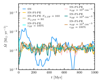
Figure 11: The SFR as a function of time for the fiducial galaxy, showing variants of SN-PI-PE with various alterations to the star formation prescription, as described in the main text. Unless otherwise noted in the legend, parameters have their default values. SN is also shown for reference. The SFR is largely insensitive to our trialled alterations (the lines mostly lie on top of each other), though it becomes slightly more bursty with increased density threshold.

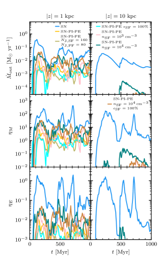
Figure 12: Outflow rates as a function of time for the fiducial galaxy, showing variants of SN-PI-PE with various alterations to the star formation prescription, as described in the main text. Unless otherwise noted in the legend, parameters have their default values. SN is also shown for reference. Outflow rates through 1 kpc are slightly increased when the density threshold for star formation is increased, however there are still no significant outflows through 10 kpc.

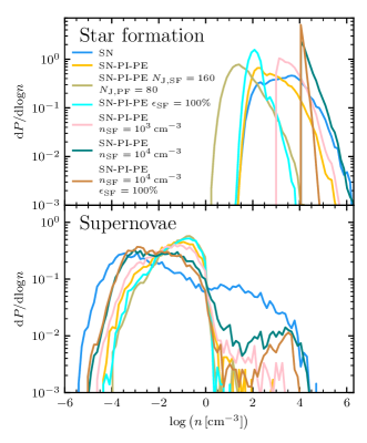
Figure 13: PDFs of the densities of the birth site of stars (top) and SN locations (bottom) for our fiducial galaxy, showing variants of SN-PI-PE with various alterations to the star formation prescription, as described in the main text. Unless otherwise noted in the legend, parameters have their default values. SN is also shown for reference. As is to be expected, increasing the density threshold for star formation shifts the PDF for birth sites to higher densities. Increasing the SF efficiency skews the PDF to lower densities and removes the high density tail. There is only a marginal impact on the PDF of SN sites, although increasing the density threshold produces a small population of SN occurring between $1-10^{4}\,\mathrm{cm^{-3}}.$

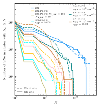
Figure 14: The number of SNe progenitors born (dashed line) or exploding (solid line) in clusters greater than some number, $N$, for our fiducial galaxy, showing variants of SN-PI-PE with various alterations to the star formation prescription, as described in the main text. Unless otherwise noted in the legend, parameters have their default values. SN is also shown for reference. Increasing the density threshold for star formation increases clustering but increasing the star formation efficiency (marginally) decreases it. No SN-PI-PE simulation produces as many large clusters as SN.

We have so far not discussed how our results depend on the adopted star formation prescription, which can often have a significant impact on the way in which stellar feedback operates in galaxy formation simulations. The choice of a prescription is complex and non-trivial, particularly at this mass resolution where it is difficult to ascertain how much of the process of the gravitational collapse is resolved and what physics is truly captured vs. how much of this process must be in the domain of the sub-grid model. The literature is currently full of many and varied ways of approaching this problem. A full census of these approaches and a parameter study is beyond the scope of this work, though we wish to pursue this in the future. For now, we limit ourselves to trialling some coarse alterations to our default prescription in order to assess the degree to which our results are dependent on our default choice.

As mentioned in Section 3.2, we use a Jeans mass threshold for star formation and adopt the same threshold value, $N_{\mathrm{J,SF}}=8$ as Hu et al. (2017), who simulate a very similar galaxy to ours. However, that work uses a particle mass of $4\,\mathrm{M_{\odot}}$ but an SPH kernel of 100 particles, meaning that in real terms their adopted threshold mass is a factor of 20 larger than ours. We therefore trial a value of $N_{\mathrm{J,SF}}=160$ to compensate. For this simulation, we also adopt a non-thermal pressure floor to prevent gas from collapsing much further than this threshold, forcing the Jeans mass to be resolved by $N_{\mathrm{J,PF}}=80$ cells. In other simulations, we trial the addition of a density threshold in combination with our Jeans mass threshold. As noted previously, our default threshold leads to the onset of star formation at around $100\,\mathrm{cm^{-3}}$. We therefore experiment with using a density threshold of $10^{3}\,\mathrm{cm^{-3}}$ and $10^{4}\,\mathrm{cm^{-3}}$.

The final parameter in our model that we vary is the small scale star formation efficiency, $\epsilon_{\mathrm{SF}}$. The default choice in our simulations is 2%. However, many in the literature argue for the use of a much higher (or variable) value in combination with more restrictive thresholds for star formation. We therefore try a simulation with our default threshold but increase the efficiency to 100%. We also perform a simulation with the addition of a density threshold at $10^{4}\,\mathrm{cm^{-3}}$ and the increased efficiency of 100%.

Fig. 11 shows the SFR for these simulations, along with our fiducial SN and SN-PI-PE runs for reference. All SFRs are very similar to each other and the fiducial SN-PI-PE, no matter which of the SF prescriptions is adopted, with nearly identical average values. This is due to efficient self-regulation of the SFR by feedback. However, the two simulations with the additional density threshold of $10^{4}\,\mathrm{cm^{-3}}$ have a more bursty SFR than the fiducial simulation (the standard deviation of the SFR, averaged in 10 Myr bins, from 200 Myr onwards is $2.48\times 10^{-4}\,\mathrm{\mathrm{M_{\odot}}\,yr^{-1}}$ for the fiducial simulation in contrast to $4.59\times 10^{-4}\,\mathrm{\mathrm{M_{\odot}}\,yr^{-1}}$ and $4.85\times 10^{-4}\,\mathrm{\mathrm{M_{\odot}}\,yr^{-1}}$ for the simulations with $n_{\mathrm{SF}}=10^{4}\,\mathrm{cm^{-3}}$ with a star formation efficiency of 2% and 100%, respectively). This is also true for the $n_{\mathrm{SF}}=10^{3}\,\mathrm{cm^{-3}}$ simulation, albeit to a lesser extent (a standard deviation of $3.30\times 10^{-4}\,\mathrm{\mathrm{M_{\odot}}\,yr^{-1}}$). Nonetheless, none of the simulations with all feedback channels switched on match the degree of burstiness produced by the fiducial SN simulation (a standard deviation of $1.24\times 10^{-3}\,\mathrm{\mathrm{M_{\odot}}\,yr^{-1}}$, much of which originates from a few large amplitude bursts rather than the shorter timescale fluctuations about the mean seen in the SN-PI-PE simulations). Fig. 12 shows the outflow rates for the same simulations. Through 1 kpc, there is a trend for outflow rates to increase as the SF density threshold is increased. The $10^{4}\,\mathrm{cm^{-3}}$ threshold simulations have outflow rates that are $\sim 2-5$ times larger and show a similar increase in terms of mass loadings. There is a marginal trend for decreased outflow rates with increased $\epsilon_{\mathrm{SF}}$. The SN simulation still produces significantly stronger outflows than any of the SN-PI-PE variants. This is even more obvious at 10 kpc: while the increased $\epsilon_{\mathrm{SF}}$ simulations are able to drive a small amount of material through 10 kpc, this is still at a significantly sub-unity mass loading factor and is several orders of magnitude weaker than the SN simulation.

The most obvious impacts of changing the SF prescription can be seen when examining the local environment of star particle birth and SN events, and their clustering properties. Fig. 13 shows the distribution of the density at which stars were born and at which SNe exploded for the simulations, in an analogous manner to Fig. 8. As is to be expected, changing the criteria for which gas is eligible for star formation has a noticeable impact on the PDFs of the ambient density at which stars are formed. Relaxing the Jeans mass threshold from $N_{\mathrm{J,SF}}=8$ to 160 results in the onset of star formation shifting to lower densities by roughly an order of magnitude to a few $\mathrm{cm^{-3}}$ with a peak at $25\,\mathrm{cm^{-3}}$. The use of a density threshold in addition to the Jeans mass threshold results in a sudden onset of star formation at that threshold, as expected. The PDFs also peak at the threshold value (for either $10^{3}$ or $10^{4}\,\mathrm{cm^{-3}}$) with a tail extending to higher densities. The effect of increasing the small scale star formation efficiency to $\epsilon_{\mathrm{SF}}=100\%$ has a significant impact on both the simulation with the fiducial threshold and the $10^{4}\,\mathrm{cm^{-3}}$ density threshold. In the former case, the peak of the distribution is reduced by a factor of a few but, more significantly, the extent of the high density tail is substantially reduced by over an order of magnitude. For the higher density threshold case, increasing $\epsilon_{\mathrm{SF}}$ does not shift the peak of the distribution (since it cannot go any lower than the threshold), but the distribution is narrowed significantly with the majority of star formation occurring within a factor of a few of the threshold. This effect can be thought of as a result of the relative reduction of the gas consumption time for gas at the same density by a factor of 50 as $\epsilon_{\mathrm{SF}}$ is increased from 2% to 100%, resulting in stars being formed at lower densities and preventing gas from collapsing far beyond the density threshold.

The influence of varying the SF prescription on the distribution of ambient densities where SN explode is not as significant. Broadly speaking, all the PDFs are very similar to the fiducial SN-PI-PE simulation, with most SN occurring in gas between $10^{-4}-1\,\mathrm{cm^{-3}}$. The fiducial SN-PI-PE simulation, the run with a lower Jeans mass threshold, the higher SF efficiency or a density threshold of $10^{3}\,\mathrm{cm^{-3}}$ all have a peak at around $0.1\,\mathrm{cm^{-3}}$, while the highest density threshold simulations have a slightly broader distribution. The similarities show that the photoionization feedback is able to clear away dense gas prior to SNe occurring to roughly the same extent despite the variations in where the stars were born. There is a slight exception to this in the simulations with a higher SF density threshold. These include a small population of SNe exploding at high density (in star forming gas) in addition to the main low density distribution. This is most pronounced for the $n_{\mathrm{SF}}=10^{4}\,\mathrm{cm^{-3}}$, $\epsilon_{\mathrm{SF}}=2\%$ simulation. These events represent the stars that have been born in the most dense gas, such that photoionization feedback has been unable to clear dense gas from their environment before the SNe occur.

We carry out the same clustering analysis as demonstrated in Section 5.5 on these simulations. In Fig. 14 we show the resulting cumulative distribution of cluster membership as a function of cluster size for both SN progenitors at birth and when they explode. There is a clear trend that increasing (decreasing) the density at which star formation begins, either by altering the Jeans mass threshold or using an additional density threshold, results in increased (decreased) clustering of SN progenitors at birth. There are a few related reasons for this. The primary cause appears to be that if a collapsing clump of gas is prevented from forming stars until it reaches a higher density, the SFR will be higher when it does pass the increased threshold. This mean that it is able to form relatively more stars before the cloud is quenched by the pre-SN feedback (in this case photoionization), resulting in larger clusters. As mentioned in the previous paragraph, another contributing factor is that the photoionization feedback is less efficient at higher densities. It should however be noted that with a higher density threshold, the pre-SN feedback does not have to drop the local density as much in order to prevent star formation. It should also be mentioned that the density dependence of other pre-SN feedback channels not included here (e.g. radiation pressure) are likely to be different. Finally, if gas collapses to higher densities prior to forming stars, clumps of dense gas are more likely to fragment into multiple smaller clumps. This produces clusters with fewer members than a single, larger monolithic cloud but the mean spatial separation between stars in a given cluster will be smaller.

There is a similar and related trend for the dependence on $\epsilon_{\mathrm{SF}}$. As shown in Fig. 13, the increased small scale efficiency results in a reduction in the number of stars being born at high density. This leads to a reduction in clustering for the reasons given above. However, because increasing $\epsilon_{\mathrm{SF}}$ results in a higher SFR at a given density, it produces a higher temporal (as opposed to spatial) clustering. This effect will be washed out to some extent by the variation in stellar lifetimes between stars in the same cluster which is likely to be much larger than the relative decrease in time between sequential stars being born. If we compare the two simulations with the fiducial SF threshold, we see that the birth sites of SN progenitors are less clustered with $\epsilon_{\mathrm{SF}}=100\%$ than the fiducial $2\%$. Making the equivalent comparison for the $n_{\mathrm{SF}}=10^{4}\,\mathrm{cm^{-3}}$ simulations, we find that the number of SN progenitors in a cluster is slightly greater for the higher efficiency simulation, until the cluster size is larger than $\sim 10$ at which point the reverse is true. The sensitivity to the choice of $\epsilon_{\mathrm{SF}}$ is therefore less pronounced than the previously mentioned relation to star formation threshold. It is also important to note that the precise details of the differences between the simulations are subject to our particular choice of $t_{\mathrm{link}}$ and $l_{\mathrm{link}}$ so only general trends should be inferred.

As was shown for the fiducial simulations, the clustering of the birth sites of progenitors directly translates into the relative clustering of the resulting SN events, with a reduction in clustering as stars wander away from their birth clusters. Thus, the trends we described above also apply to the clustering of the SNe themselves. Comparing to Fig. 11 and Fig. 12 we see that, as with the fiducial simulations, a correlation between increased SN clustering and both bursty SFR and larger outflows exists, at least in a general sense. The simulations with the highest SF density threshold have the greatest degree of clustering, corresponding to more and larger SN superbubbles than the fiducial SN-PI-PE simulation. The propensity to form superbubbles more readily also manifests in the marginally broader distribution of ambient densities of SN sites as seen in Fig. 13.

It is also instructive to compare to the fiducial SN simulation. Firstly, it should be noted that all of these simulations produce roughly the same number of SNe in total as the fiducial SN simulation. When we increase the onset density for star formation by a factor of 100 via the additional SF density threshold, we are able to achieve the same or marginally greater degree of clustering for birth sites (in terms of number of SN progenitors that are a member of a cluster of a given size) with all feedback channels switched on as the SN only feedback simulation, but only for cluster sizes smaller than a few 10s of members. Beyond this cluster size, even these SN-PI-PE simulations show a rapid decline in cluster membership while SN produces a relatively large proportion of its SN progenitors in clusters with as many as 100 members. This is reflected in the significantly burstier SFR of the SN simulation but more obviously in its larger outflow rates. Another phenomenon shown in Fig. 13 is that despite having a similar level of cluster membership for $N_{\mathrm{cl}}\lesssim 20$ for birth sites, the high SF density threshold SN-PI-PE simulations have much lower values for SN events themselves when compared to the fiducial SN simulation. This is because a smaller cluster is more vulnerable to having a significant portion of its stars wander away than a larger cluster. This is partly to do with the depth of the gravitational potential of the cluster, but is driven more by the reduction in the significance of a single star leaving the cluster and the relative proportion of stars on the ‘surface’ of the cluster. SN produces larger clusters of SN progenitors at birth than the high density SF threshold SN-PI-PE simulations so its SN event clustering is not as impacted by stars wandering away.

To summarise this section, we have demonstrated that the influence of the star formation prescription on the degree of clustering is subdominant when compared to the reduction of clustering by our pre-SN feedback (specifically photoionization). Because the ability of SNe to drive outflows is primarily determined by the level of clustering in our simulations, this means that the outflow rates have a much stronger dependence on whether photoionization feedback is included or not rather than the choice of star formation prescription.

6 Discussion

6.1 Effectiveness of photoionization feedback

Given how strongly photoionization affects the outcome of our simulations, it is worth examining whether the details of our model are reasonable. In terms of numerical robustness, we have tested our short-range photoionization scheme extensively and found that our results are stable over a wide range of model parameter choices and algorithmic variations. We discuss this in detail in Appendix C. However, besides the details of the implementation, we must also consider the extent to which a Strömgren type approximation such as ours is applicable. This approximation essentially assumes that every ionizing photon emitted contributes to the photoionization rate, implicitly assuming that the escape fraction through a cell is zero if it is eligible to be considered by the algorithm. Note that the escape fraction of ionizing photons in a given pixel is not forced to be zero, since it can extend to its maximum permitted value (having potentially ignored hot or low density cells) without exhausting the photon budget. Our improved HealPix method can cope with low density channels out of a host cloud giving a non-zero escape fraction, but only if they can be resolved by the pixel, otherwise the mass biasing error will be encountered. However, simply switching to a more sophisticated RT scheme does not necessarily completely solve this problem, since the inhomogeneous density structure of the GMC around the source must still be resolvable both in a hydrodynamical sense and by the RT scheme. Nevertheless, having gained the benefits of the cost effectiveness of our sub-grid radiation scheme (allowing us to perform the large parameter study in this paper), it would be instructive to perform a subset of these tests with full RT. In the meantime, we note that using adaptive ray-tracing simulations of H ii regions in GMCs with various properties, Kim et al. (2019) find that the cumulative escape fraction prior to the first SNe (the most relevant timescale for our purposes) ranges between $5-58\%$. This perhaps indicates that while our scheme may maximize the ability of H ii regions to disrupt star forming clouds with a de-facto close to zero escape fraction prior to the first SNe, we may not be drastically overestimating this effect.

The one remaining uncertainty is the extent to which star formation could persist in dense clumps that survive the general destruction of the cloud and for how long. If this phenomenon was significant, it would act to extend the transition period of the cloud from a star forming to a quenched state, potentially reducing the de-clustering impact of the radiation. Coherent clumps that are dense enough to shield against the radiation will not be destroyed by our scheme, nor will star formation within them be curtailed. However, this assumes that the internal structure of the GMC is sufficiently well resolved to give the correct density structure. Even though we adopt a very high resolution by the standards of galaxy formation simulations, it is still very difficult to resolve this internal structure. Our scheme therefore likely tends towards the maximal impact of ionizing radiation on the clustering, although it is difficult to estimate the magnitude of this effect.

6.2 The non-linear nature of combining feedback channels

Driven by the success of theories of galaxy regulation by stellar feedback developed over the last several decades, there has been a trend towards the inclusion of increasing numbers of mechanisms by which stars can influence their host galaxies. In addition to SNe, perhaps the most highly studied form of stellar feedback, the effects of stellar winds, photoionization, photoheating, radiation pressure and cosmic rays, for example, have been included in recent models (see the examples given in Section 1). Naively, one might expect that the more stars are able to inject energy into their surroundings, the greater the impact on their host galaxies. This would represent a simple additive stacking of the impacts of feedback channels. In reality, the picture has been shown to be more complicated because the various forms of feedback act on different length and time scales. For example, stellar winds and photoionization can dramatically alter the properties of the nearby ISM and local star formation but they are unable to have the large scale reach provided by SNe, which are able to create superbubbles and drive galactic outflows. In practice, different forms of feedback are predicted to interact in a complex manner, with pre-processing of the ISM by early (pre-SN), local feedback influencing the ability of the subsequent SN feedback to impact the galaxy and its surroundings. Often in the context of the evolution of whole galaxies, this is thought about in terms of non-SN feedback playing a supporting role, clearing out dense gas and enabling SN feedback to operate with maximum efficiency. In this way, while the stacking effect is highly non-linear and very dependent on context (e.g. the properties of the galaxy being considered), it still increases the overall impact on the galaxy with increasing numbers of feedback channels. Of course, this is still an oversimplification and it is recognized that adding additional feedback channels can in some circumstances reduce the impact of SN feedback by regulating the SFR to a lower level, thus reducing the SN rate.

What we have demonstrated in this work is an example of a more subtle manner by which including additional feedback mechanisms can reduce the impact of SN feedback. Our SN feedback and photoionization schemes are both capable of regulating the global SFR to approximately the same time-averaged value, representing an almost two order of magnitude reduction from the no feedback case. Combining all of our feedback channels leads to only a relatively small additional reduction in the SFR. The average SN rate is essentially the same across all the feedback regulated simulations, within a factor of a few. Yet the introduction of photoionization feedback dramatically suppresses the ability of SNe to form superbubbles and drive strong outflows. We have demonstrated that this suppression comes about not because of a reduction in the number of SNe but by a significant reduction of their clustering in space and time. Even though the pre-processing of the ISM by photoionization results in a larger fraction of SNe occurring in low density environments, where in an individual sense they should be more efficient, the reduction of clustering that this pre-processing causes inhibits the growth of superbubbles and the ability of SNe to work together and break out of the disc. While this effect will be dependent on the exact galactic context and the specific form of feedback considered (we have already discussed uncertainties in our photoionization scheme and the extent to which it might be maximally efficient), the potential for a similar reduction in clustering exists for any pre-SN feedback channel (e.g. photoionization, stellar winds, radiation pressure) if it is efficient at disrupting star forming regions. Also, note that while we have used the terms cloud and cluster somewhat loosely in this work, the pre-SN feedback need not disrupt entire GMCs to create this effect, rather dense star forming sub-clumps, thus reducing the overall efficiency of star formation in the GMC.

6.3 Implications for coarser resolution simulations

We stress that the effect described in the previous section is only resolvable in our simulations because our star particle mass is close to the mass of the individual massive stars. Thus, it is possible for the first few massive stars in a small collapsing region of gas to prevent the birth of additional massive stars. As the star particle mass is increased, the production of stars is quantised into larger chunks, washing out this effect. In other words, the star particle mass enforces a minimum cluster size. Given that approximately one SNe is produced for every $100\,\mathrm{M_{\odot}}$ of stars, the minimum cluster size of a $1000\,\mathrm{M_{\odot}}$ star particle is already 10. Only a few percent of SNe in our SN-PI-PE occur in clusters of 10 or more (by our definition of a cluster). Thus, ignoring other impacts of coarsening resolution, we would not have been able to see a reduction in clustering to the level that we do if our star particle mass was $1000\,\mathrm{M_{\odot}}$. Increasing the star particle mass to $10^{4}\,\mathrm{M_{\odot}}$, a reasonably competitive resolution for Milky Way mass galaxy simulations, results in a minimum cluster size of 100 SNe. Only $\sim 10\%$ of the SNe in our most clustered simulations (SN and SN-PE) are members of clusters that large. Of course, in larger mass galaxies than our dwarfs, disc properties may well give rise to larger clusters, but our point stands: the ability to form smaller clusters is precluded.

In addition to the enforcement of a minimum cluster size, using a star particle mass much larger than the mass of individual massive stars completely removes the ability to observe the impact of pre-SN feedback on clustering. As described above, we have demonstrated that pre-SN feedback that is strong enough to efficiently clear star forming gas will enhance the efficiency of individual SNe by reducing the ambient ISM density but will reduce clustering in the process by quenching star formation. However, when a more massive star particle is formed, a cluster of SN progenitors is already safely contained within it. The pre-SN feedback (which is already enhanced due to the presence of all the massive stars concentrated in the same location and born at exactly the same time) can then sweep away the local ISM after a large quantum of stellar mass has already been formed. Thus the positive impact of strong pre-SN feedback on supernova efficiency (the reduction of local density) is gained without the penalty of reduced clustering. It is important to note that this remains true even with the use of individually time-resolved SNe. While the SNe may be treated one by one, the entire SN budget of the star particle is guaranteed at the moment of its creation.

It should be apparent that when galactic outflows are produced by a highly abstracted sub-grid model, such as those used in large volume cosmological simulations (see Section 1 for examples), it does not matter that SN clustering is not resolvable. Those details should already be encapsulated in the model, either explicitly by design or implicitly by tuning. However our findings suggest that when simulations are carried out at an intermediate resolution, such that more than one SNe is likely to be produced per star particle ($m_{\mathrm{part}}\gtrsim 100\,\mathrm{M_{\odot}}$), the interplay between pre-SN and SN feedback is unlikely to be correctly resolved.

6.4 Comparison to selected other works

Rosdahl et al. (2015) contains simulations of a galaxy (their ‘G8’ model) with similar properties to our ‘heavy’ galaxy with various combinations of SN and radiation feedback, provided by a moment based RT scheme. They use a grid-based code, ramses-rt (Teyssier 2002; Rosdahl et al. 2013; Rosdahl & Teyssier 2015). However, their resolution of 18 pc and star particle mass, $600~{}\mathrm{M_{\odot}}$, are significantly coarser than ours. They found that radiation feedback was able to suppress star formation to a similar level as SN feedback, with photoionization and photoheating dominating over radiation pressure. They found their radiation feedback did not amplify the efficiency of SN feedback. They find mass loading factors of $~{}0.1$ across $0.2R_{\mathrm{vir}}$ (8.2 kpc), even for SN feedback alone, although it is acknowledged that they are most likely not resolving SNe with their thermal dump feedback prescription. As with our simulations, the inclusion of photoionization feedback leads to a reduction in outflow rates, both in absolute terms and in mass loading factors. This may be at least partially caused by the overall reduction in SFR rather than the sensitivity to clustering which we observe. It is unlikely that with their resolution this effect would be observable, particularly as they note that they cannot resolve H ii regions properly. Interestingly, while not having much impact on the SFR, the inclusion of radiation pressure leads to the outflow rates being restored to their SN-only levels.

Hu et al. (2017) perform simulations of dwarf galaxies with SN feedback, spatially varying photoelectric heating and a Strömgren type approximation for photoionization similar to ours (although it is a spherical approach rather than our new HealPix based scheme). They use a modified form of the SPH code gadget-3 (Springel 2005; Hu et al. 2014) with a gas particle mass of $4\,\mathrm{M_{\odot}}$ with 100 neighbouring particles in the support radius of the SPH kernel. It is difficult to compare resolutions, but Hu (2019) finds that this is sufficient to produce convergent wind properties when the only feedback channel is SNe in the form of a thermal dump. It is noted however that they begin to slightly under-resolve the D-type expansion of H ii regions in a uniform density medium of $100\,\mathrm{cm^{-3}}$. As shown in Section 3.3.3, we resolve this accurately, so our ability to resolve our H ii region dynamics is at least as good, if not slightly better.

In common with our findings, in their fiducial galaxy (which is most similar to our low-$\Sigma$ system), the various feedback channels can regulate the SFR to roughly the same value (within a factor of a few). In contrast to us, they find photoelectric heating alone is also able to strongly suppress star formation, albeit at the cost of realistic galaxy properties. This increased effectiveness relative to our findings could be a consequence of their adoption of a higher dust-to-gas ratio in combination with a slightly different scheme for modelling FUV attenuation (see our discussion in Section B). Although photoionization by itself is not shown, the additional reduction in SFR when it is added to the SN feedback is comparable to what we find. Their mass loading factors measured close to the disc (2 kpc) for the SN feedback only simulation appear to be significantly lower than ours, as well as being substantially smoother. The addition of photoionization feedback only reduces the outflow rates slightly in absolute terms, but the mass loading factor remains the same (the slightly lower SFR compensating). Based on their plots of the distribution of the local density where SN explode, their photoionization feedback clears away dense gas to the same degree that ours does, with essentially no SNe occurring in gas more dense than $1\,\mathrm{cm^{-3}}$. In their ‘compact’ galaxy (which is most similar to our fiducial system), only the inclusion of photoionization is capable of regulating the SFR, resulting in a smooth, steady SFR much like we find in our simulations. The SN only simulation experiences runaway star formation at the start of the simulation.

Emerick et al. (2018) simulate a halo with $M_{\mathrm{vir}}=2.48\times 10^{9}\,\mathrm{M_{\odot}}$ (a quarter the mass of our system) with a gas disc of $2\times 10^{6}\,\mathrm{M_{\odot}}$ (2.6% the mass of our disc) with the grid-based code enzo (Bryan et al. 2014). They model a similar set of physics to us (with the addition of stellar wind feedback and the following of molecular species with grackle), but use adaptive ray-tracing radiative transfer for their ionizing radiation, which also includes radiation pressure (unlike our scheme). They have a maximum spatial resolution of 1.8 pc. With our target cell mass of $20\,\mathrm{M_{\odot}}$, we have equivalent spatial resolution in gas at a density of $200\,\mathrm{cm^{-3}}$ which, coincidentally, is their star formation threshold density. They also track individual massive stars so they should in principle be able to resolve the same effects of pre-SN feedback on clustering that we do. It is therefore instructive, despite the substantial differences in galaxy properties, to qualitatively compare our results. They report that the addition of radiation feedback to the SN feedback results in a drop in SFR of roughly a factor of 5. However, the no RT simulation is halted after only $\sim 100$ Myr, so it is unclear if the SFR would drop to a lower, steady state after the initial transient phase, as in our simulations. The no RT simulation appears to be driving similar strength outflows to the full RT simulation before it is terminated, although at a slightly smaller mass loading factor. Interestingly, when the RT is limited to 20 pc, the outflows are substantially suppressed. However, when the full long range RT is used, the outflow rates are restored to (and slightly exceed) the levels seen in the no RT simulation. This appears to be caused by radiation forming and/or maintaining channels of low density gas out of the disc plane through which outflows can escape, rather than relying on SNe themselves to achieve breakout. A possible interpretation in the framework of our findings, therefore, is that the radiation reduces the effectiveness of SNe on small scales by reducing clustering, but is able to compensate for this effect by making it easier for SNe to break out. We must therefore consider that the inclusion of long range radiation in our simulations may produce similar results, although it is difficult to predict how the compensatory facility of the long range radiation scales with system mass (or perhaps more importantly, gas surface density). In Appendix D we trial a simple tree-based scheme for long range photoionization feedback (similar to that deployed in Hopkins et al. 2018b) and find that it does not result in the opening or maintaining of channels. However, we note that this is a necessary consequence of sources in tree-based schemes emitting isotropically (without introducing substantial additional complexity). Emerick et al. (2020) expands the analysis of Emerick et al. (2018) by turning various feedback channels on and off. The key points of the earlier work that we describe above are maintained, but it is useful to note that the results are largely unaffected by the absence of radiation pressure.

Agertz et al. (2020) find a qualitatively similar behaviour to us in cosmological zoom-in simulations of a $M_{\mathrm{vir}}\left(z=0\right)=10^{9}\,\mathrm{M_{\odot}}$ halo. In the absence of radiation feedback, SF is bursty and drives strong outflows while including it results in a more gentle evolution. This predominantly leaves a signature on the mass-metallicity relation.

As part of the FIRE-2 suite of cosmological zoom-ins, Hopkins et al. (2020) find that early feedback is necessary to avoid over-clustering of SNe and a resulting ‘blowout’, qualitatively supporting the phenomenon that we report here. The magnitude of the effect and the relative importance of a given form of early feedback varies as a complex function of galaxy mass. The FIRE-2 approach is to use $\epsilon_{\mathrm{SF}}=100\%$ (in combination with restrictive SF criteria), on the premise that the early feedback acts to regulate the effective efficiency to the percent level. While an in depth study of SF prescriptions is beyond this work, we note that this makes the assumption that the early feedback is resolved correctly. At their mass resolution ($250-5.6\times 10^{4}\,\mathrm{M_{\odot}}$ for haloes between $M_{\mathrm{vir}}\left(z=0\right)\sim 10^{9}-10^{12}\,\mathrm{M_{\odot}}$) H ii regions are at best marginally resolved. Additionally, as discussed in Section 6.3, large star particle masses will enhance burstiness. It should also be noted that in Section 5.6 we showed that our results are relatively robust to the choice of $\epsilon_{\mathrm{SF}}$. Hopkins et al. (2020) also find that in dwarf galaxies the UV background plays a substantial role in smoothing out SF, providing an external method to reduce SN clustering. In our idealized galaxy setup we are largely insensitive to the UV background, but this is likely because we have a disc full of gas capable of self-shielding in place at the beginning of the simulation. Thus, it is important to note that while idealized non-cosmological simulations are very useful for gaining physical intuition, they do not capture the reality of a full cosmological context with an evolving galactic potential and inflows of gas.

6.5 Are additional physical processes necessary to restore outflow rates?

The SN-driven galactic winds in our dwarf galaxies are significantly curtailed when we add photoionization feedback. Mass loading factors at 1 kpc are between 10-100 in the former case, but are reduced by approximately an order of magnitude. The strong outflows through 10 kpc are absent. However, it is difficult to directly compare our results to observations. It is challenging to observe outflows from low-mass galaxies because of the intrinsically low surface brightness. Observations are typically limited to starburst galaxies (Martin 1999; Heckman et al. 2015; Chisholm et al. 2017; McQuinn et al. 2019) and are usually restricted to a small distance from the ISM (much less than $\sim 0.1R_{\mathrm{vir}}$). The multiphase nature of galactic outflows also complicates the comparison between simulations and observations. In particularly extreme starbursts, the mass loading factor close to the ISM can reach $\sim 60$ (Heckman et al. 2015). In a sample of less extreme starburst galaxies, McQuinn et al. (2019) find mass loadings in the range $0.1-7$. Given that our SN-PI-PE galaxies are not starbursts, our mass loadings at 1 kpc are still marginally consistent with the observations. Nonetheless, strong outflows from low-mass galaxies are frequently required by theory. They are used to explain low baryon fractions, inefficient star formation and the enrichment of the CGM low-mass systems with metals (see e.g. Mori et al. 2002; Governato et al. 2007; Brooks et al. 2007; Shen et al. 2014; Ma et al. 2016a). In a cosmological setting, Smith et al. (2019) showed that if feedback is unable to consistently clear dense gas from the centre of dwarf galaxies at high-redshift, they can become overwhelmed with inflowing material, leading to runaway star formation. Strong, bursty outflows are also posited as a mechanism to prevent the formation of stellar bulges and dark matter cusps (Governato et al. 2010; Pontzen & Governato 2012).

We therefore consider the extent to which additional physics omitted from our idealised simulations could compensate for the reduction in outflow rates that we see and reconcile our results with other theoretical expectations. We discussed the limitations of our short-range feedback scheme in the previous sections, noting that it potentially represents the maximal reduction of SN clustering. We also noted that longer range radiation may assist in the production of SN-driven outflows by creating and/or maintaining low density channels out of the ISM. Any additional feedback processes must do so without contributing to the de-clustering of the SNe. Thus, simply increasing the available pre-SN feedback budget will not necessarily enhance outflow rates. If pre-SN feedback channels can carve ‘chimneys’ out of GMCs without significantly disrupting star formation, then SNRs may be able to escape the clouds along paths of least resistance. Rogers & Pittard (2013) demonstrate this phenomenon with stellar winds, while Garratt-Smithson et al. (2018) show similar behaviour with jets from HMXBs. However, easing the SNR breakout from the birth cloud does not necessarily mean that disc breakout is achieved.

As we noted in Section 3.3, we do not treat binary stellar evolution in this work, while in reality approximately half of massive stars reside in binary systems (Sana et al. 2013). Binarity can impact the lifetimes and luminosities of stars relative to single stellar evolution, largely via mass transfer between the stars. Relative to a population of single stars only, this results in a modest increase in overall ionizing photon budget but also extends the production of ionizing radiation to later times (Eldridge & Stanway 2009; Zhang et al. 2013; Stanway et al. 2014; Stanway et al. 2016; Götberg et al. 2017, 2018). It can also give rise to a population of late time ($\sim 50-200$ Myr) core-collapse SNe, although this population only makes up approximately 15% of the total (Zapartas et al. 2017). It is unclear how these two phenomena would alter our results. However, because star forming clouds are likely to have been dispersed by the time major deviations from a population of single stars become apparent (see e.g. Ma et al. 2016b), it is probable that the impact on SN clustering and outflow generation would be weak.

A non-negligible fraction of OB stars are ejected from their birth sites by either dynamical interactions within their natal cluster or by SNe within OB binary systems (see e.g. Blaauw 1961; Poveda et al. 1967; Portegies Zwart 2000; Fujii & Portegies Zwart 2011; Eldridge et al. 2011; Oh et al. 2015). These runaway stars can travel 100s of parsecs before exploding as SNe. As we mentioned in Section 3.3, we do not include this phenomenon, although sub-grid models for runaways with various degrees of sophistication have been included in previous galaxy formation simulations (see e.g. Ceverino & Klypin 2009; Ceverino et al. 2014; Zolotov et al. 2015; Kim & Ostriker 2017, 2018). The inclusion of runways is found to increase the production of hot gas and drive stronger outflows in Ceverino & Klypin (2009) and Andersson et al. (2020). However, at much higher resolution, Kim & Ostriker (2018) see no such effect with Kim et al. (2020a) positing that the trend seen in the formerly mentioned works are due to an inability to resolve SNe properly in dense gas.

It is unclear what impact the inclusion of runaway OB stars would have on our results. On the one hand, they would further decrease the spatial clustering of SNe, further hindering the creation of superbubbles that can achieve breakout. However, ejecting massive stars from star forming regions may reduce the efficiency with which ionizing radiation can halt star formation. As has been previously noted, removing SN progenitors from dense star forming gas increases the efficiency of the subsequent SN but, as shown in Fig. 8, SNe already occur in low density gas when we include ionizing radiation. Of more relevance than the local ambient density may be the column density out of the disc. A SN bubble originating in the low density pocket of an H ii region may still have to sweep through significant dense gas in order to achieve breakout, thus requiring a cluster of SNe. By contrast, a SN originating from a progenitor thrown into a void within the disc or upwards out of the disc plane would find it easier to break out of the disc but would consequently have less gas available to entrain into an outflow. It is therefore difficult to estimate what the net effect of runaways would be, but it seems likely that it would only have a minor impact on our findings either way.

It is possible that the inclusion of cosmic rays (CRs) created by SNe could result in stronger outflows. CRs suffer less adiabatic loss than thermal gas and are not radiated away during the snowplough phase of SNR expansion. This means they can increase the momentum imparted by a SNR to a significant degree (Diesing & Caprioli 2018). Uhlig et al. (2012) demonstrated that CRs can drive strong outflow in low mass galaxies. However, this wind driving mechanism is sensitive to the details of CR transport (see Dashyan & Dubois 2020, and references therein).

It is also possible that our low outflow rates are simply an unavoidable consequence of the idealized nature of our simulations. Our initial conditions do not produce a starburst state. Given that observed galactic winds from low-mass systems are essentially limited to starburst galaxies, perhaps it is not surprising that we do not see strong winds in our simulations. In a realistic cosmological environment, inflows and mergers can drive gas into the centres of galaxies, resulting in highly spatially and temporally clustered star formation. This could overcome the de-clustering ability of local photoionization and create strong bursts of feedback capable of driving outflows.

Finally, while the general trends displayed in this work are highly informative, we caution that the precise outflow values at 10 kpc are somewhat uncertain. As previously mentioned, our idealised setup lacks a CGM (other than material thrown out of the disc by outflows) with which an outflow would otherwise interact. Additionally, while our high mass-resolution allows us to capture feedback process in the ISM, (pseudo)-Lagrangian approaches such as ours can suffer from a lack of spatial resolution in outflows because inter-particle/cell separation is tied to local density (adaptive mesh refinement (AMR) codes that use a density-based refinement criteria will also experience this effect to some degree). This issue is exacerbated when the mass outflow rate at small distances is low (even when well resolved at that location) because this drops the overall density normalisation of the wind at all radii (see e.g. Chevalier & Clegg 1985). Thus, while we are confident that our SN feedback is well resolved within the ISM (see the convergence study in Smith et al. 2018), it is possible that the difference in outflow properties at 10 kpc between simulations with and without photoionization feedback is enhanced by resolution effects. Simultaneously resolving the dense gas of the ISM (including star formation and the localised origins of stellar feedback) and the subsequent evolution of winds outside of the disc in a convergent manner likely requires an alternative (de)-refinement strategy for high specific energy gas beyond the standard constant-mass approach. This is beyond the scope of this work, but is an active area of research within the SMAUG consortium.

7 Summary and conclusions

In this work, we introduced several new methods for treating stellar feedback implemented in the code Arepo. We explicitly populate star particles with individual stars by sampling the IMF. This means we can link stellar feedback to the stars themselves, rather than using IMF averaged values as is more commonly done. In combination with our high baryonic mass resolution this allowed us to properly capture the clustered nature of stellar feedback. SN feedback is included using the scheme first demonstrated in Smith et al. (2018). We implemented two new sub-grid models for radiation feedback that allow us to include these effects at a fraction of the expense of full RT, making large parameter studies with many simulations possible. We included photoelectric heating with a spatially varying FUV field, using a tree-based method that assumes largely optically thin transport with local extinction. We included photoionization and photoheating in H ii regions around massive stars with an improved overlapping Strömgren approximation scheme, solving the balance between ionizing photons and recombination in individual angular pixels. This reduces the vulnerability to the mass biasing error experienced by previous similar schemes used in the literature.

We presented a suite of 32 simulations of isolated $M_{\mathrm{vir}}=10^{10}\,\mathrm{M_{\odot}}$ galaxies with a baryonic mass resolution of $20\,\mathrm{M_{\odot}}$ using our new feedback schemes. We focused primarily on studying the interplay between the different feedback channels and their relative impact on galaxy properties, particularly SFRs and outflow rates. We also explored the dependence of our results on baryon fraction, as well as examining the robustness of our sub-grid schemes in detail. Our main findings are as follows:

• We find that either SN or photoionization feedback acting alone are able to suppress star formation by approximately the same amount in a time averaged sense, resulting in an approximately two order of magnitude reduction in average SFRs relative to the no feedback case. However, SN feedback produces a much burstier star formation history. Photoelectric heating has negligible impact. Combining the feedback channels results in an additional small suppression of SFRs, but this is insignificant compared to the impact of either SN or photoionization alone.

• Along with the burstier star formation, SN feedback without photoionization causes greater disruption to the disc, forming large superbubbles that break out and drive strong outflows. When photoionization feedback is added, such large superbubbles are no longer present and outflow rates are significantly reduced, despite approximately the same number of SNe occurring.

• The inclusion of photoionization feedback dramatically reduces the clustering of SNe in space and time by disrupting star forming clouds before they can build up large clusters of massive stars. This inhibits the production of SN superbubbles that are capable of breaking out of the disc, thus reducing outflow rates. It also causes the smoother SFRs, since the star formation is predominantly suppressed by relatively gentle, local disruption of dense gas rather than by the disruption of large regions of the disc. This phenomenon is in principle not just limited to photoionization feedback, but could be caused by any form of pre-SN feedback that efficiently destroys star forming clouds.

• This modulation of SN clustering by early feedback can only be captured because our star particle mass is close to the masses of individual SN progenitors. Using a more massive star particle (i.e. forming stars in larger discrete units) enforces a minimum cluster size, even if SNe are individually time resolved. It reduces the ability to resolve the suppression of SN clustering by early feedback. This has implications for the robustness of claims to resolve the coupling between different forms of stellar feedback in simulations with star particle masses orders of magnitude greater than the individual massive stars.

• Our results are insensitive to variations in the adopted star formation prescription, including increasing the threshold density or small scale efficiency parameter.

• As demonstrated in Appendix A, our findings hold qualitatively when the baryon fraction of the galaxy is increased or decreased by a factor of two in either direction.

• Our new model for H ii regions is extremely robust to variations in parameters or algorithmic changes. However, we note that it can potentially overestimate the ability of ionizing radiation to disrupt star formation in GMCs if dense substructure is not properly resolved.

• Other physics missing from our simulations could compensate for the reduction in SN clustering, thus increasing outflow rates. These include longer range radiation and/or cosmic rays. We also note that the lack of strong outflows in our dwarf galaxies could simply arise from our idealised setup, with a more realistic cosmological environment potentially inducing starburst events that can overcome the de-clustering effect of the local photoionization feedback.

We have therefore shown that the interactions between different forms of stellar feedback is complex. Adding additional early feedback does not necessarily result in an increase in the ability of SNe to drive galactic winds because it can also reduce the clustering of SNe. In our idealized dwarf galaxy, this phenomenon results in a strong suppression of outflow rates when ionizing radiation is included alongside SN feedback. An interesting future avenue of research would be to investigate this effect in more massive galaxies. However, as we detail above, the baryonic mass resolution must be close to the masses of individual stars for the impact on clustering to be properly captured which is likely to be prohibitively computationally expensive. It would also be worthwhile to carry out a similar study in a cosmological environment, particularly to examine how the clustering of SNe affects outflow rates at high redshift. In a companion work (Smith et al. 2020b in prep.), we will use a similar set of simulations to demonstrate how the impact of ionizing radiation can be overestimated if star particles have IMF-averaged luminosities rather than explicitly sampled stellar inventories.

Data Availability Statement

The data underlying this article will be shared on reasonable request to the corresponding author.

Appendix A Dependence on galaxy properties

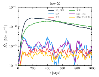
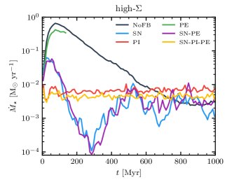
Figure 15: SFR as a function of time for the six realisations of our low-$\Sigma$ (top) and high-$\Sigma$ (bottom) galaxies. The results are qualitatively similar to the fiducial galaxy. NoFB and PE once again produce runaway star formation. PE is halted after a short time for the high-$\Sigma$ for reasons of computational expense. SN and SN-PE undergo a substantial burst of star formation followed by a quenching event as they settle from their initial conditions. PI and SN-PI-PE result in comparable relative reductions in star formation to the fiducial simulations, once again with smooth star formation histories.

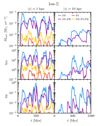
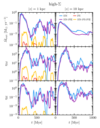
Figure 16: Mass outflow rates, mass and energy loadings for the low-$\Sigma$ (left) and high-$\Sigma$ (right) galaxies through planes at 1 kpc and 10 kpc from the disc. The results are similar to the fiducial galaxy, although the outflow rates increase with increased gas surface density. Without the photoionization feedback, SNe are able to drive strong outflows through 10 kpc. When it is added (SN-PI-PE), outflows through 1 kpc are much reduced and essentially no material reaches 10 kpc.

We now explore the extent to which the results from our fiducial galaxy simulations apply to our low-$\Sigma$ and high-$\Sigma$ galaxies. Recall that these galaxies have the same total system mass but have half or twice the baryonic mass in the disc, respectively, with the same scale radius. Fig. 15 shows the SFR for the low-$\Sigma$ and high-$\Sigma$ galaxies, with the six combinations of feedback channels for each galaxy. The general trends exhibited for our fiducial galaxy carry over into these simulations. Photoelectric heating is again unable to regulate star formation much beyond the NoFB case. In the high-$\Sigma$ galaxy, once the runaway star formation has been confirmed we stop this simulation to avoid additional computational expense. Simulations SN and SN-PE again give very similar SFRs. They show a significant reduction in star formation from the simulation without feedback and show a very bursty star formation history. In the high-$\Sigma$ examples, SN and SN-PE experience a much larger initial transient than our other two galaxies, significantly disrupting the disc, although their SFR settles after 500 Myr.

In both galaxies and in common with the fiducial simulations, PI shows a much smoother star formation history and suppresses the SFR to approximately a similar degree as the SN only simulations. Likewise, adding SNe and photoelectric heating to the photoionization in the SN-PI-PE simulations results in a slight additional reduction. There is a slight variation in the relative efficiency of the SN and photoionization feedback between our different galaxies. In the fiducial case, when averaged over the last 500 Myr, both channels regulated the SFR to the same level independently of each other. In the low-$\Sigma$ galaxy, the PI simulation gives a 22% lower average SFR than the SN run. This is a marginal decrease so we must be cautious about putting too much emphasis on this finding given the potential for the effects of stochasticity where bursty feedback is involved. The ranking of efficiencies reverses in the high-$\Sigma$ galaxy, with SN feedback alone giving a 57% lower average SFR over the last 500 Myr than photoionization feedback (and is 35% lower than the full feedback case). However, a large part of this difference is driven by the variation in the early stages of the simulations. The large burst of star formation and subsequent feedback in the SN simulation in the initial transient phase results in a non-negligible quantity of gas being thrown out of the galaxy (as we shall show in more detail below). This means that that the gas reservoir available for star formation in the last 500 Myr is substantially reduced, likely driving a significant amount of the differences between the average SFR for the simulations with or without photoionization feedback.

Fig. 16 shows outflow rates for the low-$\Sigma$ and high-$\Sigma$ galaxies. The results are similar to the fiducial simulation, in a relative sense. The PI simulations drive a small amount of material through 1 kpc. Simulations SN and SN-PE are again able to drive strong outflows, with mass loadings of 10 or greater through 1 kpc for both low-$\Sigma$ and high-$\Sigma$ galaxies. In the low-$\Sigma$ galaxy, it takes 500 Myr for the first substantial outflows to begin being driven through 10 kpc, eventually achieving mass loadings between $1-10$. In the heavier galaxy, the initial burst of feedback at the start of the simulation drives a very strong outflow through 10 kpc. After 500 Myr, relatively constant outflows with mass loading factors averaging between a factor of a few to 10s are present. Again, including all the feedback channels (SN-PI-PE) results in substantial reduction in outflows. There is a trend for increasing outflow rate in absolute terms through 1 kpc as the disc mass increases, but a slight reduction in mass loading factor. There are no outflows over 10 kpc.

Thus, it can be seen that our general trends identified with the fiducial galaxy also transfer to changes in the baryon fraction of a factor of 2 in each direction. We have not varied the total system mass in this work, although it would be an instructive experiment for the future. The ease with which outflows can be driven out to large radii (in a relative sense) is dependent on the halo potential, thus the sensitivity to SN clustering that we have described may change. However, as we describe in more detail in Section 6, we would ideally need to keep a comparable resolution to make a reasonable comparison.

Appendix B The effectiveness of photoelectric heating

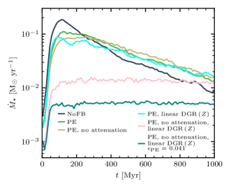
Figure 17: Star formation rates for our realisation of our fiducial galaxy showing the sensitivity of photoelectric heating to various changes to our default scheme. Removing attenuation of the FUV radiation by dust has little impact. Using a higher dust-to-gas ratio (by adopting a linear dependence on metallicity instead of the broken power-law of Rémy-Ruyer et al. (2014)) has no impact unless FUV attenuation is switched off, in which case the SFR is suppressed by an order of magnitude (but is still an order of magnitude higher than simulations with SN or photoionization feedback). Fixing $\epsilon_{\mathrm{PE}}$ at its upper limit of 0.041 suppresses the SFR by an additional factor of $\sim 2.5$. NoFB is also shown for reference.

In Fig. 17 we show SFRs for our fiducial galaxy without feedback, our standard photoelectric heating scheme and four variations on the scheme. Firstly, we examine the extent to which the strength of the photoelectric heating is influenced by our prescription for the attenuation of the FUV radiation by dust. As described in Section 3.3.2, we use a very simplistic measurement of the dust column density around a source based on the local Jeans length. As can be seen in Fig. 17, if we do not attenuate the FUV radiation at all we see very little additional suppression of star formation relative to the standard case. This indicates that the dust-to-gas ratio (DGR) in our galaxy is sufficiently low that attenuation is not relevant.

This brings us to the other source of uncertainty: the DGR itself. As stated in Section 3.3.2, we adopt an observationally motivated broken power-law scaling with metallicity taken from Rémy-Ruyer et al. (2014). Rather than the linear scaling with metallicity often assumed in simulations, this includes a steepening of the relation at low metallicity. Thus, for our adopted initial ISM metallicity of $0.1\,\mathrm{Z_{\odot}}$, we obtain a DGR of 1.1% of the MW value, an order of magnitude lower than a simple linear scaling would give. With such a low DGR, it is perhaps not surprising that photoelectric heating is not very efficient. In Fig. 17 we also show the results from PE simulations using a linear relationship between metallicity and DGR by extending the high metallicity portion of the Rémy-Ruyer et al. (2014) broken power law down to all metallicities. We show this for simulations with and without our standard FUV attenuation prescription. When the attenuation is included, the resulting SFR is similar to the simulations with our standard DGR. However, when no attenuation is included, the SFR is suppressed by almost an order of magnitude, reaching a steady state for the duration of the simulation. It is still an order of magnitude higher than our SN and PI simulations, but in combination with the other feedback channels it could potentially have an impact. This indicates that the gains in the photoelectric heating rate due to increased dust are largely cancelled out by the increased attenuation of the radiation under our scheme. The strength of this effect implies that if there is a sufficiently high DGR such that photoelectric heating is relatively efficient, then the results may well be sensitive to the dust attenuation prescription.

Finally, we maximize the effects of photoelectric heating by performing a run with the linear DGR-metallicity scaling and no attenuation but additionally fix the photoelectric heating efficiency to the highest possible value our scheme allows, $\epsilon_{\mathrm{PE}}=0.041$. Recall that $\epsilon_{\mathrm{PE}}$ normalises the relationship giving the heating rate as a function of the FUV energy intensity and the DGR (see eq. 8). $\epsilon_{\mathrm{PE}}$ depends on the temperature and electron number density. The latter is exceedingly hard to capture without accurately modelling the complex processes that contribute to it in cold gas. We therefore adopt a fit as a function of density to the results of Wolfire et al. (2003) (see e.g. eq. 9) for our fiducial simulations. The maximum efficiency of 0.041 is reached in gas of density $730\,\mathrm{cm^{-3}}$ or higher. Using this efficiency at all densities results in the heating rate in 1, 10 and 100 $\mathrm{cm^{-3}}$ gas being enhanced by a factor of 4.7, 2.7 and 1.6, respectively, relative to our fiducial scheme. This results in the SFR being suppressed even further to an average of $5.2\times 10^{-3}\,\mathrm{M_{\odot}}\,\mathrm{yr}$. This is within a factor of a few of the fiducial SN and PI simulations. This suggests that adjustments to the $\epsilon_{\mathrm{PE}}$ can make a substantial difference to the effectiveness of photoelectric heating, in combination with other assumptions about the DGR and attenuation. We believe that the use of a fixed value for $\epsilon_{\mathrm{PE}}$ must be treated with care, despite it being a commonly adopted approach. For reference, Forbes et al. (2016) use an equivalent value of 0.065 while Kim & Ostriker (2017) use 0.009. Hopkins et al. (2018b) use the efficiency as a full function of temperature and electron abundance from Wolfire et al. (2003) but it is unclear whether they resolve the complex chemistry that determines the electron abundance with sufficient accuracy in the relevant gas phases.

Appendix C Robustness of the short-range photoionization model

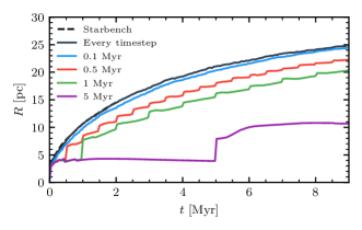
Figure 18: We repeat the test described in Section 3.3.3 and shown in Fig. 1 but vary the frequency with which the photoionization flagging algorithm is carried out. All simulations shown use our default HealPix scheme. As the recalculation is carried out less frequently, the D-type expansion is stalled relative to the Starbench RT benchmark results. The recalculation must be carried out at least every 0.1 Myr to be in reasonable agreement with the benchmark.

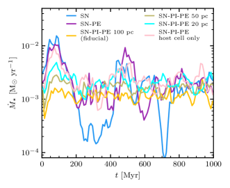
Figure 19: The SFR as a function of time for the fiducial galaxy, showing SN-PI-PE runs where the size of H ii regions, $r_{\mathrm{ion,max}}$ is limited to 100 pc (as normal), 50 pc, 20 pc or confined to the cell hosting the star particle. SN and SN-PE are also shown for reference. Decreasing $r_{\mathrm{ion,max}}$ results in a marginal increase in the SFR.

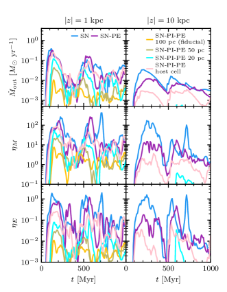
Figure 20: Outflow rates as a function of time for the fiducial galaxy, showing SN-PI-PE runs where the sizes of H ii regions are limited to 100 pc (as normal), 50 pc, 20 pc or confined to the cell hosting the star particle. SN and SN-PE are also shown for reference. Only confining photoionization to the host cell results in a substantial increase in the outflow rates through 10 kpc.

Given the impact of photoionization feedback on our results, it is worthwhile to examining the robustness of our short range photoionization feedback model. There are a variety of different parameters that can be altered in the sub-grid model that could potentially have an impact. We have extensively explored these parameter choices as well as alternative methods of implementing the model. We find that the following alterations have negligible impact (if any) on our results in general, but specifically in relation to SFRs and outflows:

• Removing the density threshold for a cell to be considered in the algorithm, $n_{\mathrm{photo,min}}$, results in no change. H ii regions frequently extend outwards to their 100 pc limit into low density gas around dense clouds, but this gas is either hot enough already to be ignored or is briefly prevented from forming new clouds. Increasing $n_{\mathrm{photo,min}}$ has only a minor impact, resulting in roughly a factor of 2 increase in the average SFR when it is increased to $100~{}\mathrm{cm^{-3}}$ but no impact on outflow mass loadings. There is no physical reason for it to be set at this density or higher.

• Increasing the threshold temperature above which gas is ignored by the algorithm from its fiducial value of $T_{\mathrm{photo,max}}=1.05\times 10^{4}\,\mathrm{K}$ to $10^{5}\,\mathrm{K}$ has no effect.

• Increasing the number of angular pixels used from 12 to 48 has negligible impact. Increasing to 192 pixels (the next level of refinement) shows only a marginal increase in the SFR. At this point, the ionizing photon rate is divided into sufficiently small portions that it is hard for a pixel to ionize a cell. However the initiation of a D-Type expansion by the host cell (even though it is not properly resolved) often begins driving dense material away such that the density drops enough for pixels ionize cells. Examination of individual H ii regions also reveals frequent occurrence of the previously predicted error whereby the majority of pixels pass through the closest cells to the source, since we only check that the mesh generating point lies in the pixel, not for the intersection of the pixel with a cell as in a true ray tracing scheme. Thus the densest gas around sources can be bypassed, with a very noisy distribution of photoionized cells spread over a large volume when pixels happen to encounter mesh generating points of cells. Although not tested, further increase of angular resolution is likely to result in reduced effectiveness of the photoionization feedback by rendering all pixels unable to ionize gas cells, rather than any real gains in accuracy due to the increased resolution.

• Switching to a more traditional spherical scheme does not qualitatively alter our results on a global scale, although individual H ii regions have erroneous shapes (for the reasons described in Section 3.3.3).

• Reducing the frequency with which the extent of H ii regions are calculated (our fiducial choice is to do this for all sources every fine time-step) has no effect, until the time between recalculations becomes longer than $\sim$0.1 Myr. As discussed in Section 3.3.3, this is due to the ionization front lagging behind the expansion of the over-pressurised bubble, resulting in unphysical stalling of the D-type expansion. We demonstrate this in Fig. 18, where we repeat the idealised experiment from Section 3.3.3 with various refresh rates. Likewise, changing from synchronous to asynchronous recalculations (described in Section 3.3.3) with the aim of reducing any potential ‘flickering’ has no impact.

• We trialled including a more conservative time-step limiter such that all cells within 100 pc of a gas cell with non-zero SFR or a star particle containing a massive star have their Courant condition evaluated assuming the maximum of either their actual sound speed or that which they would achieve upon being photoionized, in order to ensure that they were prepared for the arrival of an ionizing source. This had no impact.

• Our results are insensitive to whether the hydrodynamic properties of a cell are updated immediately upon being flagged as photoionized or upon completion of their current hydrodynamic time-step.

• Our results are unaffected by minor alterations to our IMF scheme such as reducing the maximum stellar mass to $50\,\mathrm{M_{\odot}}$ or increasing the minimum stellar mass explicitly tracked from our default $5\,\mathrm{M_{\odot}}$ to $8\,\mathrm{M_{\odot}}$. This is because the contribution to the total ionizing luminosity for stars outside these limits is negligible.

• Decreasing the temperature assigned to photoionized gas from $10^{4}\,\mathrm{K}$ to $7\times 10^{3}\,\mathrm{K}$ (as used in some other works) has no discernible impact on our results.

• To rule out the very unlikely possibility that pre-processing of the ISM by photoionization feedback was somehow interfering with the behaviour of our sub-grid SN model, we performed a simulation with our mechanical feedback scheme replaced by a simple thermal dump of energy into the host cell of the star particle (along with the ejecta). This produced near identical results because all SNe were well resolved due to the reduction in ambient density by the photoionization scheme (see Fig. 8).

The one parameter choice that does have an impact on our results is the maximum radius we permit the H ii region to expand to. Our default choice is 100 pc. In Fig. 19, in addition to our fiducial SN, SN-PE and SN-PI-PE simulations, we show the SFR for our fiducial galaxy with the maximum H ii radius restricted to 50 pc and 20 pc. We also show the impact of allowing only the cell hosting the ionizing star particle to be flagged as photoionized, representing the most extreme restriction our resolution allows. Fig. 20 shows outflow rates for the same simulations. Once again, taking the average SFR in the last 500 Myr of the simulation to allow the disc to settle, we find that reducing the maximum radius to 50 pc results in an increase of 40% and to 20 pc produces an increase of 75%. There is therefore a trend for increasing SFR with decreasing maximum radius, which one might intuitively expect, although it is small relative to other sources of uncertainty and numerical noise. The majority of this increase comes from rare, relatively large clusters of massive stars near the centre of the galaxy, with the vast majority of H ii regions not reaching this limit. This is particularly obvious when comparing the spatial extent of star formation activity in the first 100 Myr when the SFR is dominated by a single, large clump of star forming gas as the disc settles from the ICs. We stress that the limit is not being reached by stars in isolation but rather by stars already sitting in an H ii region formed by several other stars, reaching out to ionize neutral cells just beyond the current ionization front. However, the further away from the source the angular pixel extends the more vulnerable it becomes to mass biasing effects, even though our HealPix scheme improves significantly upon previous schemes, substantially reducing our errors. The sensitivity to this parameter is a drawback of Strömgren type approximation schemes as the choice is somewhat arbitrary. Hu et al. (2017) choose an empirically determined maximum value of 50 pc to avoid mass biasing at long range (using a simple spherical scheme which is more vulnerable to this), based on observations of the typical size of H ii regions in dwarf galaxies (e.g. Cormier et al. 2015). However, as we show, reducing our fiducial value to 50 pc makes little difference. As far as outflows are concerned, reducing the maximum radius has only a small impact beyond the initial bursts of outflow as the disc settles. Decreasing the limit to 50 pc results in approximately the same outflow rate through 1 kpc from 500 Myr onwards as the fiducial simulation. Decreasing further to 20 pc does produce a burst of enhanced outflow at late times, but at the cost of a marginally higher SFR, resulting in an increase in mass loadings of only a factor of a few. These changes have essentially no impact on the outflow rates through 10 kpc.

Restricting the photoionization scheme to only act on cells hosting ionizing stars results in a SFR that is relatively consistent with turning off the scheme altogether, producing a bursty SF history and an average SFR over the last 500 Myr that is consistent with SN-PE within 3%. The simulation does not have as large amplitude bursts as those produced by SN-PE but strong conclusions should not be drawn from this due to the possibility of numerical noise. The outflow rates at 1 kpc are relatively consistent with SN-PE but there is reduction in the outflow rates through 10 kpc of a factor of a few. We also see a small reduction in the clustering of SNe. Thus, it seems that even restricted to one cell the photoionization model has a small impact. For reference, with our target cell mass of $20\,\mathrm{M_{\odot}}$, cells have diameters of 2.27 pc and 0.49 pc at densities of $100\ \mathrm{cm^{-3}}$ and $10^{4}\ \mathrm{cm^{-3}}$, respectively. However, because newly formed star particles are formed at the density peak of a collapsing cloud, if they ionize the cell in which they reside the resulting over-pressure is frequently able to hinder further collapse, resulting in a slight reduction of clustering, as described in Section 5.5.

Appendix D Long Range Photoionization scheme

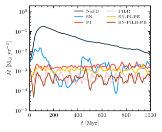
Figure 21: The SFR as a function of time for the fiducial galaxy, showing runs with our long range photoionization scheme activated (in addition to the fiducial short range scheme). We show both full physics with long range photoionization (SN-PILR-PE) as well as photoionization alone (PILR). NoFB, SN, PI and SN-PI-PE runs are also shown for reference. Adding the long range photoionization scheme results in additional suppression of star formation. SNe are subdominant.

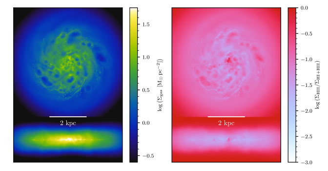
Figure 22: Projections of the fiducial galaxy after 1 Gyr with all stellar feedback channels switched on and the long-range photoionization scheme active (SN-PILR-PE). Left: gas column density. Right: Ratio of the surface densities of ionized hydrogen to total hydrogen (effectively a projected ionization fraction). Compared to SN-PI-PE (see Fig. 3 and 4) the disc is much smoother and thicker.

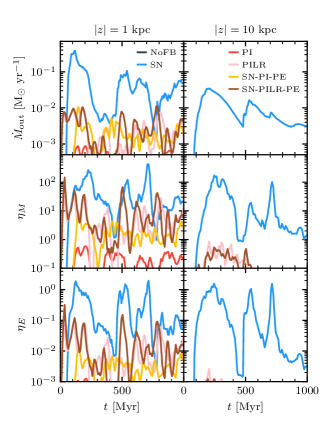
Figure 23: Outflow rates as a function of time for the fiducial galaxy, showing runs with our long range photoionization scheme activated (in addition to the fiducial short range scheme). We show both full physics with long range photoionization (SN-PILR-PE) as well as photoionization alone (PILR). NoFB, SN, PI and SN-PI-PE runs are also shown for reference.

The short-range photoionization feedback scheme used in the main body of this work treats the impact of ionizing radiation on the neutral gas around the source i.e. the creation of localised H ii regions. As mentioned in Section 6, it is possible that the effects of ionizing radiation at longer range may promote stronger outflows by creating or sustaining pre-existing low density channels out of the disc, compensating for the suppression of outflows caused by the H ii regions to some degree. Such a phenomenon is reported in a lower mass galaxy by Emerick et al. (2018). A self-consistent treatment of ionizing radiation outside the regime where a Strömgren type approximation is valid should properly be treated with a full RT scheme, which is beyond the scope of this work. However, we wish to examine whether a basic approximation, such as that used by Hopkins et al. (2018b), can produce this effect. The approach taken in that work is that attenuation of the ionizing radiation only occurs locally to the source and at the point of reception. In other words, it makes the strong assumption that there is a negligible column density of neutral gas along the majority of the path of the radiation. This scheme is therefore constructed in a similar fashion to our treatment of the spatially varying FUV field and likewise has the advantage of incurring negligible computational expense.

We count leftover ionizing photons from the short-range scheme that arise because the ionization front in a pixel has reached $r_{\mathrm{ion,max}}$. This occurs when a pixel has achieved breakout into hot and/or low density gas or because the ionizing source is not embedded in dense gas. Note that this will result in a sensitivity to the choices of $r_{\mathrm{ion,max}}$ and (to a lesser extent) $n_{\mathrm{photo,min}}$, although we do not explore this for the purposes of this work. The mean energy of the leftover photons, obtained as a function of the source star’s mass as compiled in Emerick et al. (2019), is then used to obtain an emergent luminosity in the ionizing band. Using the same method that we employ in our photoelectric heating scheme, we obtain the energy density in the ionizing band from these emergent sources at each location in space by summing up individual contributions with the gravity tree. In our current implementation, this radiation is emitted from the sources isotropically i.e. it does not take into account the varying levels of attenuation in different directions obtained via our HealPix method in the short-range scheme, a potentially significant shortcoming. The addition of a directional dependence to the emitted ionizing flux, while feasible, would require substantial modifications to the tree algorithm.

We then boost the ionization and heating rates from the UV background experienced by each cell by a factor $f_{\mathrm{ion}}=1+u_{\mathrm{ion,\star}}/u_{\mathrm{ion,UVB}}$, where $u_{\mathrm{ion,\star}}$ and $u_{\mathrm{ion,UVB}}$ are the local energy densities in the ionizing band from the emergent sources and the UV background respectively. This therefore makes the simplifying assumption that the UV background has the same spectrum as our stellar sources. The heating and ionization rates are then attenuated by the self-shielding prescription as normal. This part of the scheme is achieved by modifying the publicly available version of grackle to incorporate this boost factor. Note that this approach will result in an inconsistency between the strength of ionizing radiation assumed when calculating the metal cooling tables and that used for the primordial species. Since this scheme only takes into account attenuation of the ionizing radiation field at the source (via the short-range scheme) and via the self-shielding approximation at the point of reception, it ignores attenuation along the line of sight, potentially overestimating the strength of the radiation field in the ionizing band. The boost factor is not applied to gas which is flagged as photoionized by the short range scheme, although this makes little difference.

We perform two simulations of our fiducial galaxy with the long range photoionization scheme switched on (in addition to the short range scheme). PILR just uses photoionization feedback, while SN-PILR-PE adds SN feedback and photoelectric heating. Fig. 21 shows the SFR for these simulations along with our fiducial NoFB, SN, PI and SN-PI-PE runs. Adding the long range scheme results in an additional suppression of the SFR, with averages after 500 Myr of $5.2\times 10^{-4}\,\mathrm{M_{\odot}}$ and $4.5\times 10^{-4}\,\mathrm{M_{\odot}}$ for PILR and SN-PILR-PE, respectively. These are 29% and 39% of the average SFRs for their equivalent fiducial simulations, PI and SN-PI-PE. The averages of PILR and SN-PILR-PE are sufficiently close that it appears that the SN feedback is now somewhat subdominant to the ionizing radiation.

Fig. 22 shows projections of the gas surface density and ionization fraction of SN-PILR-PE after 1 Gyr. By comparing to Fig. 3 and 4, we can see that using the long range photoionization scheme results in a smoother, thicker disc and a significant reduction in the amount of neutral gas. In Fig. 23 we can see that adding the long range scheme does not lead to a noticeable increase in outflows. The absolute outflow rate across 1 kpc for both PILR and SN-PILR-PE is comparable to SN-PI-PE, but these is primarily composed of a slow fountain as the disc thickens. There are still no significant outflows through 10 kpc, in contrast to SN.

We therefore find that accounting for long range ionization radiation using this simple tree-based scheme does not reproduce the behaviour seen by Emerick et al. (2018) with more rigorous ray-tracing based RT, in which channels out of the disc are created and/or maintained. Instead, we see a more general increase in heating and ionization throughout the disc resulting in the suppression of star forming clumps. In hindsight, this is not unexpected given the construction of the scheme. We find that pixels in the short range scheme predominantly achieve breakout out of the disc plane, rather than in the plane, when the sources are embedded in dense gas. Even when a source is sitting in the expanding hot bubble of a nearby SNe, 100 pc (our adopted $r_{\mathrm{ion,max}}$) sight-lines pointing out of the disc are typically clearer of neutral gas. With an accurate treatment of RT, the radiation that escapes along these sight-lines will (correctly) continue in that direction (ignoring scattering). However, with our tree-based scheme we are limited to emitting it isotropically, redistributing a significant portion of the escaping radiation back into the disc plane. This hinders the ability to maintain vertical channels of photoionized gas and unphysically enhances the disc heating and ionization rates. Upgrading our scheme to give anisotropic emission would be non-trivial. The tree is designed to sum contributions to the gravitational force (and radiation energy density in our extension) from isotropically ‘emitting’ sources that are distributed anisotropically. In other words, it is relatively simple to obtain a vector quantity at the point of reception (necessary for the gravitational force) but not to emit in a vector sense without incurring substantial penalty to both computational expense and memory requirements. Additionally, while we find that a coarse angular resolution (12 pixels in our fiducial scheme) is sufficient for our purposes in the short range scheme, a significantly higher resolution would be required for a longer range scheme.

It is also likely that the naive treatment of radiation attenuation is not accurate enough, with a comparison to a full RT scheme being necessary to confirm that the local shielding approximation is valid. Given the strength of the effect we see here, we suspect that it may not be, although we have performed no such comparison. The inability of the scheme to account for attenuation along the line of sight (other than locally) will compound the erroneous heating and ionization rates arising from the unphysical re-direction of escaping radiation into the disc plane. Hopkins et al. (2020) compared a similar scheme (which they refer to as ‘LEBRON’) to a moment based RT approach and find that global galaxy properties are comparable, even though locally there can be significant differences. However, at their mass resolution of $250\,\mathrm{M_{\odot}}$, H ii regions are only marginally resolved so small scale anisotropies in escaping radiation are unlikely to be captured with the moment based RT. In the ‘LEBRON’ scheme, their Strömgren approximation scheme for H ii regions cannot account for anisotropic distributions of neutral gas around sources, unlike our new HealPix approach, so is incapable of resolving channels through which radiation can escape from dense regions. Regardless, even if our improved short-range photoionization scheme is adopted, we find that this type of long-range photoionization model is unsuitable for capturing the effects detailed in Emerick et al. (2018), should they be physically possible in our particular galaxy.

References

- Agertz & Kravtsov (2015) Agertz O., Kravtsov A. V., 2015, ApJ, 804, 18
- Agertz et al. (2020) Agertz O., et al., 2020, MNRAS, 491, 1656
- Aguirre et al. (2001) Aguirre A., Hernquist L., Schaye J., Katz N., Weinberg D. H., Gardner J., 2001, ApJ, 561, 521
- Allende Prieto et al. (2001) Allende Prieto C., Lambert D. L., Asplund M., 2001, ApJ, 556, L63
- Allende Prieto et al. (2002) Allende Prieto C., Lambert D. L., Asplund M., 2002, ApJ, 573, L137
- Andersson et al. (2020) Andersson E. P., Agertz O., Renaud F., 2020, MNRAS, 494, 3328
- Anglés-Alcázar et al. (2020) Anglés-Alcázar D., et al., 2020, arXiv e-prints, p. arXiv:2008.12303
- Artale et al. (2015) Artale M. C., Tissera P. B., Pellizza L. J., 2015, MNRAS, 448, 3071
- Bakes & Tielens (1994) Bakes E. L. O., Tielens A. G. G. M., 1994, ApJ, 427, 822
- Bergin et al. (2004) Bergin E. A., Hartmann L. W., Raymond J. C., Ballesteros-Paredes J., 2004, ApJ, 612, 921
- Bisbas et al. (2015) Bisbas T. G., et al., 2015, MNRAS, 453, 1324
- Blaauw (1961) Blaauw A., 1961, Bull. Astron. Inst. Netherlands, 15, 265
- Bland-Hawthorn et al. (2007) Bland-Hawthorn J., Veilleux S., Cecil G., 2007, Ap&SS, 311, 87
- Bressan et al. (2012) Bressan A., Marigo P., Girardi L., Salasnich B., Dal Cero C., Rubele S., Nanni A., 2012, MNRAS, 427, 127
- Brooks et al. (2007) Brooks A. M., Governato F., Booth C. M., Willman B., Gardner J. P., Wadsley J., Stinson G., Quinn T., 2007, ApJ, 655, L17
- Bryan et al. (2014) Bryan G. L., et al., 2014, ApJS, 211, 19
- Ceverino & Klypin (2009) Ceverino D., Klypin A., 2009, ApJ, 695, 292
- Ceverino et al. (2014) Ceverino D., Klypin A., Klimek E. S., Trujillo-Gomez S., Churchill C. W., Primack J., Dekel A., 2014, MNRAS, 442, 1545
- Chevalier & Clegg (1985) Chevalier R. A., Clegg A. W., 1985, Nature, 317, 44
- Chieffi & Limongi (2004) Chieffi A., Limongi M., 2004, ApJ, 608, 405
- Chisholm et al. (2017) Chisholm J., Tremonti C. A., Leitherer C., Chen Y., 2017, MNRAS, 469, 4831
- Cormier et al. (2015) Cormier D., et al., 2015, A&A, 578, A53
- Dale et al. (2014) Dale J. E., Ngoumou J., Ercolano B., Bonnell I. A., 2014, MNRAS, 442, 694
- Dashyan & Dubois (2020) Dashyan G., Dubois Y., 2020, A&A, 638, A123
- Dashyan et al. (2018) Dashyan G., Silk J., Mamon G. A., Dubois Y., Hartwig T., 2018, MNRAS, 473, 5698
- Davé et al. (2016) Davé R., Thompson R., Hopkins P. F., 2016, MNRAS, 462, 3265
- Davé et al. (2019) Davé R., Anglés-Alcázar D., Narayanan D., Li Q., Rafieferantsoa M. H., Appleby S., 2019, MNRAS, 486, 2827
- Diesing & Caprioli (2018) Diesing R., Caprioli D., 2018, Phys. Rev. Lett., 121, 091101
- Dubois et al. (2014) Dubois Y., et al., 2014, MNRAS, 444, 1453
- Dubois et al. (2016) Dubois Y., Peirani S., Pichon C., Devriendt J., Gavazzi R., Welker C., Volonteri M., 2016, MNRAS, 463, 3948
- El-Badry et al. (2019) El-Badry K., Ostriker E. C., Kim C.-G., Quataert E., Weisz D. R., 2019, MNRAS, 490, 1961
- Eldridge & Stanway (2009) Eldridge J. J., Stanway E. R., 2009, MNRAS, 400, 1019
- Eldridge et al. (2011) Eldridge J. J., Langer N., Tout C. A., 2011, MNRAS, 414, 3501
- Emerick et al. (2018) Emerick A., Bryan G. L., Mac Low M.-M., 2018, ApJ, 865, L22
- Emerick et al. (2019) Emerick A., Bryan G. L., Mac Low M.-M., 2019, MNRAS, 482, 1304
- Emerick et al. (2020) Emerick A., Bryan G. L., Mac Low M.-M., 2020, arXiv e-prints, p. arXiv:2007.03702
- Evans (1999) Evans N. J., 1999, ARA&A, 37, 311
- Evans et al. (2009) Evans N. J., et al., 2009, ApJS, 181, 321
- Faucher-Giguere et al. (2013) Faucher-Giguere C.-a., Quataert E., Hopkins P. F., 2013, MNRAS, 433, 1970
- Federrath (2015) Federrath C., 2015, MNRAS, 450, 4035
- Ferland et al. (2013) Ferland G. J., et al., 2013, Rev. Mexicana Astron. Astrofis., 49, 137
- Ferrière (2001) Ferrière K. M., 2001, Rev. Mod. Phys., 73, 1031
- Fielding et al. (2017) Fielding D., Quataert E., Martizzi D., Faucher-Giguère C.-A., 2017, MNRAS, 470, L39
- Fielding et al. (2018) Fielding D., Quataert E., Martizzi D., 2018, MNRAS, 481, 3325
- Fielding et al. (2020) Fielding D. B., et al., 2020, ApJ, 903, 32
- Forbes et al. (2016) Forbes J. C., Krumholz M. R., Goldbaum N. J., Dekel A., 2016, Nature, 535, 523
- Fujii & Portegies Zwart (2011) Fujii M. S., Portegies Zwart S., 2011, Science, 334, 1380
- Gallegos-Garcia et al. (2020) Gallegos-Garcia M., Burkhart B., Rosen A. L., Naiman J. P., Ramirez-Ruiz E., 2020, ApJ, 899, L30
- Garratt-Smithson et al. (2018) Garratt-Smithson L., Wynn G. A., Power C., Nixon C. J., 2018, MNRAS, 480, 2985
- Garratt-Smithson et al. (2019) Garratt-Smithson L., Wynn G. A., Power C., Nixon C. J., 2019, MNRAS, 489, 4278
- Gatto et al. (2015) Gatto A., et al., 2015, MNRAS, 449, 1057
- Gentry et al. (2017) Gentry E. S., Krumholz M. R., Dekel A., Madau P., 2017, MNRAS, 465, 2471
- Gentry et al. (2019) Gentry E. S., Krumholz M. R., Madau P., Lupi A., 2019, MNRAS, 483, 3647
- Górski & Hivon (2011) Górski K. M., Hivon E., 2011, HEALPix: Hierarchical Equal Area isoLatitude Pixelization of a sphere (ascl:1107.018)
- Götberg et al. (2017) Götberg Y., de Mink S. E., Groh J. H., 2017, A&A, 608, A11
- Götberg et al. (2018) Götberg Y., de Mink S. E., Groh J. H., Kupfer T., Crowther P. A., Zapartas E., Renzo M., 2018, A&A, 615, A78
- Governato et al. (2007) Governato F., Willman B., Mayer L., Brooks A., Stinson G., Valenzuela O., Wadsley J., Quinn T., 2007, MNRAS, 374, 1479
- Governato et al. (2010) Governato F., et al., 2010, Nature, 463, 203
- Grevesse & Sauval (1998) Grevesse N., Sauval A. J., 1998, Space Sci. Rev., 85, 161
- Grudić et al. (2018) Grudić M. Y., Hopkins P. F., Faucher-Giguère C.-A., Quataert E., Murray N., Kereš D., 2018, MNRAS, 475, 3511
- Haardt & Madau (2012) Haardt F., Madau P., 2012, ApJ, 746, 125
- Habing (1968) Habing H. J., 1968, Bull. Astron. Inst. Netherlands, 19, 421
- Hayward & Hopkins (2017) Hayward C. C., Hopkins P. F., 2017, MNRAS, 465, 1682
- Heckman et al. (2015) Heckman T. M., Alexandroff R. M., Borthakur S., Overzier R., Leitherer C., 2015, ApJ, 809, 147
- Hennebelle & Iffrig (2014) Hennebelle P., Iffrig O., 2014, A&A, 570, A81
- Hernquist (1990) Hernquist L., 1990, ApJ, 356, 359
- Holweger (2001) Holweger H., 2001, in Wimmer-Schweingruber R. F., ed., AIP Conf. Proc. Vol. 598, Joint SOHO/ACE workshop “Solar and Galactic Composition”. Am. Inst. Phys., New York, pp 23–30
- Hopkins et al. (2014) Hopkins P. F., Kereš D., Oñorbe J., Faucher-Giguère C.-A., Quataert E., Murray N., Bullock J. S., 2014, MNRAS, 445, 581
- Hopkins et al. (2018a) Hopkins P. F., et al., 2018a, MNRAS, 477, 1578
- Hopkins et al. (2018b) Hopkins P. F., et al., 2018b, MNRAS, 480, 800
- Hopkins et al. (2020) Hopkins P. F., Grudić M. Y., Wetzel A., Kereš D., Faucher-Giguère C.-A., Ma X., Murray N., Butcher N., 2020, MNRAS, 491, 3702
- Hu (2019) Hu C.-Y., 2019, MNRAS, 483, 3363
- Hu et al. (2014) Hu C.-Y., Naab T., Walch S., Moster B. P., Oser L., 2014, MNRAS, 443, 1173
- Hu et al. (2016) Hu C.-Y., Naab T., Walch S., Glover S. C. O., Clark P. C., 2016, MNRAS, 458, 3528
- Hu et al. (2017) Hu C.-Y., Naab T., Glover S. C. O., Walch S., Clark P. C., 2017, MNRAS, 471, 2151
- Jaura et al. (2018) Jaura O., Glover S. C. O., Klessen R. S., Paardekooper J. P., 2018, MNRAS, 475, 2822
- Keller & Kruijssen (2020) Keller B. W., Kruijssen J. M. D., 2020, arXiv e-prints, p. arXiv:2004.03608
- Keller et al. (2019) Keller B. W., Wadsley J. W., Wang L., Kruijssen J. M. D., 2019, MNRAS, 482, 2244
- Kennicutt (1998) Kennicutt R. C., 1998, ApJ, 498, 541
- Kereš et al. (2009) Kereš D., Katz N., Davé R., Fardal M., Weinberg D. H., 2009, MNRAS, 396, 2332
- Kim & Ostriker (2015a) Kim C.-G., Ostriker E. C., 2015a, ApJ, 802, 99
- Kim & Ostriker (2015b) Kim C.-G., Ostriker E. C., 2015b, ApJ, 815, 67
- Kim & Ostriker (2017) Kim C.-G., Ostriker E. C., 2017, ApJ, 846, 133
- Kim & Ostriker (2018) Kim C.-G., Ostriker E. C., 2018, ApJ, 853, 173
- Kim et al. (2011) Kim C.-G., Kim W.-T., Ostriker E. C., 2011, ApJ, 743, 25
- Kim et al. (2019) Kim J.-G., Kim W.-T., Ostriker E. C., 2019, ApJ, 883, 102
- Kim et al. (2020a) Kim C.-G., et al., 2020a, ApJ, 900, 61
- Kim et al. (2020b) Kim C.-G., et al., 2020b, ApJ, 903, L34
- Kimm & Cen (2014) Kimm T., Cen R., 2014, ApJ, 788, 121
- Kimm et al. (2015) Kimm T., Cen R., Devriendt J., Dubois Y., Slyz A., 2015, MNRAS, 451, 2900
- Kimm et al. (2018) Kimm T., Haehnelt M., Blaizot J., Katz H., Michel-Dansac L., Garel T., Rosdahl J., Teyssier R., 2018, MNRAS, 475, 4617
- Koudmani et al. (2019) Koudmani S., Sijacki D., Bourne M. A., Smith M. C., 2019, MNRAS, 484, 2047
- Koudmani et al. (2021) Koudmani S., Henden N. A., Sijacki D., 2021, MNRAS, 503, 3568
- Kroupa (2001) Kroupa P., 2001, MNRAS, 322, 231
- Krumholz & Tan (2007) Krumholz M. R., Tan J. C., 2007, ApJ, 654, 304
- Lanz & Hubeny (2003) Lanz T., Hubeny I., 2003, ApJS, 146, 417
- Leitherer et al. (1999) Leitherer C., et al., 1999, ApJS, 123, 3
- Li & Bryan (2020) Li M., Bryan G. L., 2020, ApJ, 890, L30
- Li et al. (2015) Li M., Ostriker J. P., Cen R., Bryan G. L., Naab T., 2015, ApJ, 814, 4
- Li et al. (2020a) Li M., Li Y., Bryan G. L., Ostriker E. C., Quataert E., 2020a, ApJ, 894, 44
- Li et al. (2020b) Li M., Li Y., Bryan G. L., Ostriker E. C., Quataert E., 2020b, ApJ, 898, 23
- Ma et al. (2016a) Ma X., Hopkins P. F., Faucher-Giguère C.-A., Zolman N., Muratov A. L., Kereš D., Quataert E., 2016a, MNRAS, 456, 2140
- Ma et al. (2016b) Ma X., Hopkins P. F., Kasen D., Quataert E., Faucher-Giguère C.-A., Kereš D., Murray N., Strom A., 2016b, MNRAS, 459, 3614
- Manzano-King et al. (2019) Manzano-King C. M., Canalizo G., Sales L. V., 2019, ApJ, 884, 54
- Marinacci et al. (2019) Marinacci F., Sales L. V., Vogelsberger M., Torrey P., Springel V., 2019, MNRAS, 489, 4233
- Martin (1999) Martin C. L., 1999, ApJ, 513, 156
- Martin (2005) Martin C. L., 2005, ApJ, 621, 227
- Martin et al. (2010) Martin C. L., Scannapieco E., Ellison S. L., Hennawi J. F., Djorgovski S. G., Fournier A. P., 2010, ApJ, 721, 174
- Martizzi (2020) Martizzi D., 2020, MNRAS, 492, 79
- Martizzi et al. (2015) Martizzi D., Faucher-Giguere C.-A., Quataert E., 2015, MNRAS, 450, 504
- Martizzi et al. (2016) Martizzi D., Fielding D., Faucher-Giguère C. A., Quataert E., 2016, MNRAS, 459, 2311
- McKee & Ostriker (1977) McKee C. F., Ostriker J. P., 1977, ApJ, 218, 148
- McQuinn et al. (2019) McQuinn K. B. W., van Zee L., Skillman E. D., 2019, ApJ, 886, 74
- Mori et al. (2002) Mori M., Ferrara A., Madau P., 2002, ApJ, 571, 40
- Motwani et al. (2020) Motwani B., et al., 2020, arXiv e-prints, p. arXiv:2006.16314
- Navarro et al. (1997) Navarro J., Frenk C. S., White S. D. M., 1997, ApJ, 490, 493
- Oh et al. (2015) Oh S., Kroupa P., Pflamm-Altenburg J., 2015, ApJ, 805, 92
- Ostriker & Shetty (2011) Ostriker E. C., Shetty R., 2011, ApJ, 731, 41
- Ostriker et al. (2010) Ostriker E. C., McKee C. F., Leroy A. K., 2010, ApJ, 721, 975
- Pakmor et al. (2016) Pakmor R., Springel V., Bauer A., Mocz P., Munoz D. J., Ohlmann S. T., Schaal K., Zhu C., 2016, MNRAS, 455, 1134
- Pandya et al. (2020) Pandya V., et al., 2020, ApJ, 905, 4
- Penny et al. (2018) Penny S. J., et al., 2018, MNRAS, 476, 979
- Pettini et al. (2003) Pettini M., Madau P., Bolte M., Prochaska J. X., Ellison S. L., Fan X., 2003, ApJ, 594, 695
- Pillepich et al. (2018) Pillepich A., et al., 2018, MNRAS, 473, 4077
- Pontzen & Governato (2012) Pontzen A., Governato F., 2012, MNRAS, 421, 3464
- Portegies Zwart (2000) Portegies Zwart S. F., 2000, ApJ, 544, 437
- Poveda et al. (1967) Poveda A., Ruiz J., Allen C., 1967, BOTT, 4, 86
- Rahmati et al. (2013) Rahmati A., Pawlik A. H., Raičević M., Schaye J., 2013, MNRAS, 430, 2427
- Rémy-Ruyer et al. (2014) Rémy-Ruyer A., et al., 2014, A&A, 563, A31
- Rogers & Pittard (2013) Rogers H., Pittard J. M., 2013, MNRAS, 431, 1337
- Rosdahl & Teyssier (2015) Rosdahl J., Teyssier R., 2015, MNRAS, 449, 4380
- Rosdahl et al. (2013) Rosdahl J., Blaizot J., Aubert D., Stranex T., Teyssier R., 2013, MNRAS, 436, 2188
- Rosdahl et al. (2015) Rosdahl J., Schaye J., Teyssier R., Agertz O., 2015, MNRAS, 451, 34
- Sales et al. (2014) Sales L. V., Marinacci F., Springel V., Petkova M., 2014, MNRAS, 439, 2990
- Sana et al. (2013) Sana H., et al., 2013, A&A, 550, A107
- Schaye et al. (2015) Schaye J., et al., 2015, MNRAS, 446, 521
- Schroetter et al. (2015) Schroetter I., Bouché N., Péroux C., Murphy M. T., Contini T., Finley H., 2015, ApJ, 804, 83
- Semenov et al. (2017) Semenov V. A., Kravtsov A. V., Gnedin N. Y., 2017, ApJ, 845, 133
- Sharma et al. (2014) Sharma P., Roy A., Nath B. B., Shchekinov Y., 2014, MNRAS, 443, 3463
- Shen et al. (2014) Shen S., Madau P., Conroy C., Governato F., Mayer L., 2014, ApJ, 792, 99
- Silk (2017) Silk J., 2017, ApJ, 839, L13
- Smith (2021) Smith M. C., 2021, MNRAS, 502, 5417
- Smith et al. (2017) Smith B. D., et al., 2017, MNRAS, 466, 2217
- Smith et al. (2018) Smith M. C., Sijacki D., Shen S., 2018, MNRAS, 478, 302
- Smith et al. (2019) Smith M. C., Sijacki D., Shen S., 2019, MNRAS, 485, 3317
- Somerville & Davé (2015) Somerville R. S., Davé R., 2015, ARA&A, 53, 51
- Songaila (2005) Songaila A., 2005, AJ, 130, 1996
- Songaila (2006) Songaila A., 2006, AJ, 131, 24
- Springel (2005) Springel V., 2005, MNRAS, 364, 1105
- Springel (2010) Springel V., 2010, MNRAS, 401, 791
- Springel & Hernquist (2003a) Springel V., Hernquist L., 2003a, MNRAS, 339, 289
- Springel & Hernquist (2003b) Springel V., Hernquist L., 2003b, MNRAS, 339, 312
- Springel et al. (2005) Springel V., Di Matteo T., Hernquist L., 2005, MNRAS, 361, 776
- Stanway et al. (2014) Stanway E. R., Eldridge J. J., Greis S. M. L., Davies L. J. M., Wilkins S. M., Bremer M. N., 2014, MNRAS, 444, 3466
- Stanway et al. (2016) Stanway E. R., Eldridge J. J., Becker G. D., 2016, MNRAS, 456, 485
- Teyssier (2002) Teyssier R., 2002, A&A, 385, 337
- Uhlig et al. (2012) Uhlig M., Pfrommer C., Sharma M., Nath B. B., Enßlin T. A., Springel V., 2012, MNRAS, 423, 2374
- Vázquez-Semadeni et al. (2010) Vázquez-Semadeni E., Colín P., Gómez G. C., Ballesteros-Paredes J., Watson A. W., 2010, ApJ, 715, 1302
- Veilleux et al. (2005) Veilleux S., Cecil G., Bland-Hawthorn J., 2005, ARA&A, 43, 769
- Vogelsberger et al. (2013) Vogelsberger M., Genel S., Sijacki D., Torrey P., Springel V., Hernquist L., 2013, MNRAS, 436, 3031
- Vogelsberger et al. (2014) Vogelsberger M., et al., 2014, MNRAS, 444, 1518
- Walch et al. (2012) Walch S. K., Whitworth A. P., Bisbas T., Wünsch R., Hubber D., 2012, MNRAS, 427, 625
- Walch et al. (2015) Walch S., et al., 2015, MNRAS, 454, 238
- Wheeler et al. (2019) Wheeler C., et al., 2019, MNRAS, 490, 4447
- White & Frenk (1991) White S. D. M., Frenk C. S., 1991, ApJ, 379, 52
- Williams & McKee (1997) Williams J. P., McKee C. F., 1997, ApJ, 476, 166
- Wolfire et al. (2003) Wolfire M. G., McKee C. F., Hollenbach D., Tielens A. G. G. M., 2003, ApJ, 587, 278
- Yadav et al. (2017) Yadav N., Mukherjee D., Sharma P., Nath B. B., 2017, MNRAS, 465, 1720
- Zapartas et al. (2017) Zapartas E., et al., 2017, A&A, 601, A29
- Zhang et al. (2013) Zhang Y., Liu J., Zhang F., Han Z., 2013, A&A, 554, A136
- Zolotov et al. (2015) Zolotov A., et al., 2015, MNRAS, 450, 2327
- Zuckerman & Evans II (1974) Zuckerman B., Evans II N. J., 1974, ApJl, 192, L149