Combining Post-Circular and Padé approximations to compute Fourier domain templates for eccentric inspirals

Abstract

Observations of transient gravitational wave (GW) events with non-negligible orbital eccentricity can be highly rewarding from astrophysical considerations. Ready-to-use fully analytic frequency domain inspiral GW templates are crucial ingredients to construct eccentric inspiral-merger-ringdown waveform families, required for the detection of such GW events. It turns out that a fully analytic, post-Newtonian (PN) accurate frequency domain inspiral template family, which uses certain post-circular approximation, may only be suitable to model events with initial eccentricities $e_{0}\leq 0.2$.We here explore the possibility of combining Post-Circular and Padé approximations to obtain fully analytic frequency domain eccentric inspiral templates. The resulting 1PN-accurate approximant is capable of faithfully capturing eccentric inspirals having $e_{0}\leq 0.6$ while employing our 1PN extension of a frequency domain template family that does not use post-circular approximation, detailed in Moore, B., et al. 2018, Classical and Quantum Gravity, 35, 235006. We also discuss subtleties that arise while combining post-circular and Padé approximations to obtain higher PN order templates for eccentric inspirals.

I Introduction

Gravitational wave events that involve compact binaries in non-circular orbits are of definite interest to the functional hecto-hertz GW observatories such as the Advanced LIGO (aLIGO), Advanced Virgo (aVirgo), and KAGRA Aasi et al. (2015); Acernese et al. (2014); KAGRA collaboration (2019). This is despite the fact that all confirmed and recorded GW detections contain compact binaries inspiraling along quasi-circular orbits Abbott et al. (2019a); GraceDB (2020); Abbott et al. (2019b). In contrast, massive black hole (BH) binaries in eccentric orbits, like the one in bright blazar OJ 287 Laine et al. (2020), are promising nano-Hz GW sources for the rapidly maturing Pulsar Timing Array effortsPerera et al. (2019); Susobhanan et al. (2020). Orbital eccentricity is expected to be an important parameter for milli-hertz and deci-hertz GW astronomy that will be heralded by LISA and DECIGO, respectively Baibhav et al. (2019); Zwick et al. (2020); Sato et al. (2017).

GW events that involve non-negligible orbital eccentricities are interesting to the LIGO-Virgo-Kagra consortium, because such events should allow us to constrain possible formation scenarios for the observed binary BH coalescences and to test general relativity Romero-Shaw et al. (2019); Moore and Yunes (2020). It turns out that formation scenarios for the observed O1, O2 and O3 binary BH events roughly fall in two distinct possibilities. The first scenario involves BH binaries formed in the galactic fields via isolated binary stellar evolution Belczynski et al. (2002); Kruckow et al. (2018). These compact binaries are expected to have orbital eccentricities $\sim 10^{-4}$ when their GWs enter aLIGO frequency window Kowalska et al. (2011). Such values are substantially below the levels at which we can constrain orbital eccentricities of aLIGO and aVirgo GW events Abbott et al. (2016); Huerta et al. (2018). The second scenario involves formation of BH binaries at very close orbital separations and this is astrophysically possible in globular clusters, young star clusters, and active galactic nuclei Fragione and Bromberg (2019); Samsing (2018); Kumamoto et al. (2020); O’Leary et al. (2009); Kremer et al. (2019). These scenarios ensure that temporal evolution of BH binaries are perturbed by other compact objects leading to the development of orbital eccentricities. The fact that GW emission reduces orbital eccentricity by a factor of three when its semi-major axis shrinks by a factor of two ensures that dynamically formed compact binaries with short orbital periods can display non-negligible orbital eccentricities in the aLIGO frequency window Peters (1964). Additionally, BH binaries in such dense stellar environments can experience Kozai-Lidov resonances due to gravitational perturbations of a third BH and such a scenario can also provide eccentric BH binaries in the aLIGO frequency window Kozai (1962); Antonini et al. (2014); Randall and Xianyu (2018). It is important to note that the above two binary BH formation scenarios lead to distinct distributions for the masses and spins of binary constituents Farr et al. (2017); Arca Sedda et al. (2020). Unfortunately, GW observations from a few dozen BH binaries can not provide constraints on the most favorable formation scenarios for the so far recorded GW events.

There are on-going efforts to probe the presence of eccentric compact binary mergers in the available interferometric data sets Tiwari et al. (2016); Abbott et al. (2019c); Nitz et al. (2020); Lenon et al. (2020). Measuring orbital eccentricity of a GW event should allow us to identify the prominent formation channel for aLIGO BH binaries. This is mainly because of few detailed and realistic evolution of compact binaries in globular clusters which suggest that $\sim 10\%$ of such binaries can have eccentricities $>0.1$ when their GWs enter aLIGO frequency window Samsing (2018); Rodriguez et al. (2018). An efficient detection of such GW events and the accompanying accurate parameter estimation requires one to develop accurate and efficient eccentric IMR template families both in the time and frequency domains, similar to template families developed for quasi-circular inspirals Hannam (2014); Damour and Nagar (2016).

There are few on-going efforts to compute such template families for binary black hole systems, merging along moderately eccentric orbits Hinder et al. (2018); Huerta et al. (2018); Chiaramello and Nagar (2020); Ramos-Buades et al. (2020). These detailed investigations are being augmented by efforts that explore the search sensitivity of popular modeled and unmodeled LIGO-Virgo collaboration search algorithms to capture eccentric binary black hole coalescences, as pursued in Ref. Ramos-Buades et al. (2020). An eccentric inspiral-merger-ringdown (IMR) family that extends the very popular PhenomD templates for quasi-circular merger events Husa et al. (2016); Khan et al. (2016) will be very helpful for extending efforts of Ref. Ramos-Buades et al. (2020) and eventually searching for eccentric GW events.

A crucial ingredient to such an eccentric IMR family will be a fully analytic frequency domain GW response function for eccentric inspirals. The post-circular (PC) scheme, developed and extended in Refs. Yunes et al. (2009); Tanay et al. (2016); Moore et al. (2016); Tiwari et al. (2019), allowed one to compute fully analytic third post-Newtonian (3PN) accurate frequency domain $\tilde{h}(f)$ for eccentric inspirals by employing the method of stationary phase approximation Bender and Orszag (1999). Recall that PN approximation provides general relativity based corrections to the Newtonian dynamics of a compact binary system in terms of $(v/c)^{2}$, with $v$ denoting the orbital speed of the binary and $c$ being the speed of light in vacuum. Therefore, $3$PN corrections provide $(v/c)^{6}$ general relativity based contributions to relevant expressions and equations.

The PN-accurate PC approach provides fully analytic 3PN-accurate expressions for the orbital eccentricity and the Fourier phases of $\tilde{h}(f)$ as functions of GW frequency and involves series expansions in $e_{0}$, the value of orbital eccentricity at certain initial GW frequency, at every PN order. At present, Ref. Tiwari et al. (2019) provides the most PN-accurate $\tilde{h}(f)$ for compact binaries inspiraling along eccentric orbits while employing the PC scheme. This fully analytic frequency domain GW response function incorporates 1PN-accurate amplitude, 3PN-accurate Fourier phase as well as 3PN-accurate evolution of orbital eccentricity $e_{t}$ in terms of orbital frequency $F$, while taking into account up to $\mathcal{O}(e_{0}^{6})$ corrections at every PN order. An important feature of $\tilde{h}(f)$, given in Ref. Tiwari et al. (2019), is the incorporation of general relativistic periastron advance in orbital motion of eccentric binaries. However, it was pointed out that PC scheme based $\tilde{h}(f)$ should be applicable to eccentric inspirals with $e_{0}\leq 0.2$, especially if they incorporate only next-next-to leading order $e_{0}$ contributions Moore et al. (2018). This prompted Ref. Moore et al. (2018) to develop a semi-analytic frequency domain inspiral $\tilde{h}(f)$ that should be accurate to model eccentric inspirals with $e_{0}>0.2$. This initial investigation incorporated the effects of dominant quadrupolar order GW emission while constructing their inspiral $\tilde{h}(f)$. Thereafter, Ref. Moore and Yunes (2019) provided an inspiral eccentric $\tilde{h}(f)$ family that incorporated GW emission effects to 3PN order and outlined a way to incorporate the effect of periastron advance in the Fourier phases.

The present effort explores the possibility of extending the ability of PN-accurate PC approach to model eccentric inspirals with $e_{0}\sim 0.6$. This is influenced by the fact that the resulting $\tilde{h}(f)$ will be useful to extend the existing frequency domain PhenomD IMR templates with eccentric effects. And, there are on-going efforts to create such eccentric templates with inputs from Refs. Ramos-Buades et al. (2020) and Tiwari et al. (2019). We employ an elegant and simple re-summation technique, namely the Padé approximation as detailed in Ref. Bender and Orszag (1999), on various Taylor expanded quantities of the PC scheme based $\tilde{h}(f)$. We list below key findings of our investigations:

• We obtain Padé approximation for the two crucial quantities, required to operationalise Newtonian-order frequency-domain analytic inspiral waveform. This includes $e_{t}(F)$ that provides the frequency evolution of orbital eccentricity, and the associated Fourier phases $\Psi(F)$. The rational polynomials for these quantities were computed from their post-circular scheme counterparts that included $\mathcal{O}(e_{0}^{19})$ and $\mathcal{O}(e_{0}^{20})$ corrections, respectively.

• Our quadrupolar order Padé approximation for $e_{t}$ provides fractional relative errors that are $\leq 10^{-4}$ even for $e_{0}$ values like $0.6$. These estimates employ numerically extracted $e_{t}(F)$ values from an exact quadrupolar orbital frequency $\omega(e_{t},e_{0},\omega_{0})$ expression, present in Ref. Moore et al. (2018) (hereafter referred to as the MoRoLoYu approach).

• We developed a fully analytic quadrupolar order Padé approximation based $\tilde{h}(f)$ (Padé approximant $\tilde{h}(f)$). The usual match ($\mathcal{M}$) analysis reveals that our approximant is faithful to the MoRoLoYu inspiral $\tilde{h}(f)$ with $e_{0}\sim 0.6$.

• We extended the above two inspiral template families, namely the Padé and MoRoLoYu inspiral approximants, to 1PN order while restricting the amplitudes to the quadrupolar order. These two waveform families were also found to be faithful to each other for the classical aLIGO binaries with $e_{0}$ values $\sim 0.6$.

• We discuss possible issues that need to be tackled to extend our Padé approximant to higher PN orders. This is influenced by the discussions of Ref. Moore and Yunes (2019) and the observed discrepancies between the analytically and numerically extracted values of certain PN-accurate quantities.

We restricted our attention to $e_{0}\lesssim 0.6$ values, influenced by the Laplace limit. This limit provides the maximum value for which the usual power series in $e$ solution to the classical Kepler equation, namely $l=u-e\,\sin u$, converges Colwell (1993). Note that we employ essentially such a solution to compute the starting point of our efforts, namely Eq. (2), for the quadrupolar order GW polarization states. Interestingly, we may need to probe the existence of such a limit in PN-accurate Kepler Equation, given in Ref. Memmesheimer et al. (2004), as PN accurate version of Eq. (2) requires such a power series solution at PN orders Boetzel et al. (2017a).

Our paper is structured as follows: Sec. II provides brief descriptions of quadrupolar order PC and MoRoLoYu approaches to obtain eccentric $\tilde{h}(f)$ and introduces our Padé approximant. Various comparisons between these approaches are presented in sub-sections of Sec. II. The 1PN extensions of these approaches are presented in Sec. III that includes data analysis relevant match computations. Sec. III.4 probes subtleties that we may face while extending our Padé approximant to higher PN orders. Appendices provide some underlying equations.

II Analytic Fourier-domain eccentric GW waveform families at the quadrupolar order

We begin by summarizing how one formally obtains the frequency domain $\tilde{h}(f)$ from its time-domain counterpart, influenced by Ref. Yunes et al. (2009). How to operationalize the resulting $\tilde{h}(f)$ for two distinct approaches is described in the next two subsections. These two approaches are the fully analytic PC scheme of Ref. Yunes et al. (2009) and semi-analytic approach of Ref. Moore et al. (2018) that should be valid essentially for arbitrary initial eccentricities. Thereafter, we present our fully analytic Padé approximant to model eccentric inspirals. In what follows, we briefly summarize formulae that are required to compute FD GW response function for eccentric inspirals from its time domain counterpart. This is desirable as all the above three approaches employ these formulae.

The first step to obtain the FD GW response function $\tilde{h}(f)$ is to write down the time domain GW response (or strain) of a ground based GW detector as

$$h(t)=F_{+}h_{+}(t)+F_{\times}h_{\times}(t),$$ (1)

where $F_{+}$ and $F_{\times}$ are the antenna patterns of the interferometer that depend on certain angles, $\theta_{S}$, $\phi_{S}$ and $\psi_{S}$ that specify the declination and right ascension of the source as well as the polarisation angle ($\psi_{S}$), respectively. Further, $h_{+}(t)$ and $h_{\times}(t)$ represent the time-dependent GW polarization states at the Newtonian or quadrupolar order. Following Ref. Yunes et al. (2009), we write

$$h_{+,\times}(t)=-\frac{Gm\eta}{c^{2}D_{L}}x\sum_{j=1}^{10}\left[C_{+,\times}^{(j)}\cos jl+S_{+,\times}^{(j)}\sin jl\right],$$ (2)

and we have restricted eccentricity contributions to $\mathcal{O}(e_{t}^{8})$. The additional symbols and variables that appear in the above equation are the luminosity distance to the source ($D_{L}$), the usual PN expansion parameter $x=(Gm\omega/c^{3})^{2/3}$ while $\eta=m_{1}m_{2}/m^{2}$ gives the symmetric mass ratio of a binary with component masses, $m_{1}$ and $m_{2}$ with total mass given as, $m=m_{1}+m_{2}$. The secular orbital frequency of the binary is given by $\omega=2\pi F$. Note that $h_{+,\times}(t)$ expressions are given as a sum over harmonics ($j$) of $l$, the mean anomaly, defined as $l=n(t-t_{0})$ where $n=2\pi/P$ gives the mean motion of binary system having an orbital period of $P$ and $t_{0}$ is some initial epoch. Further, the coefficients $C_{+,\times}^{(j)}$ of $\cos jl$ and $S_{+,\times}^{(j)}$ of $\sin jl$ in Eq. (2) may be expressed as power series in certain time eccentricity parameter $e_{t}$ that appear in the Keplerian type parametric solution whose coefficients are trigonometric functions of angles $\iota,\beta$ that describe the line of sight vector in certain inertial frame Boetzel et al. (2017a). The explicit expressions for $C_{+,\times}^{(j)}$ and $S_{+,\times}^{(j)}$, accurate up to $\mathcal{O}(e_{t}^{8})$, are given by Eqs. (3.7-3.10) and (B1-B36) in Ref. Yunes et al. (2009). In general, the summation index $j$ goes to $\infty$ and the explicit expressions for $C_{+,\times}^{(j)}$ and $S_{+,\times}^{(j)}$ are written in terms of Bessel functions of first kind as given by Eqs. (9) in Ref. Moore et al. (2018). In practice, only a finite number of harmonics j are included while computing an eccentric inspiral waveform. Interestingly, the maximum number of harmonics depends on the highest order of eccentricity corrections included in the inspiral template Yunes et al. (2009). For example, a template that includes up to $\mathcal{O}(e_{t}^{s})$ eccentricity corrections should have $s+2$ as the maximum $j$ value. This is why we include $10$ harmonics in our Eq. (1), which incorporates $\mathcal{O}(e_{t}^{8})$ corrections in $e_{t}$.

It is fairly straightforward to obtain GW response function for eccentric inspirals by plugging in the expressions for $h_{+,\times}$, namely Eq. (2), into Eq. (1) and this leads to

$$h(t)=-\frac{Gm\eta}{c^{2}D_{L}}\left(\frac{Gm\omega}{c^{3}}\right)^{2/3}\sum_{j=1}^{10}\alpha_{j}\cos(jl+\phi_{j}).$$ (3)

In above equation, $\alpha_{j}$ and $\phi_{j}$ are certain combination of $F_{+,\times}$, $C_{+,\times}^{(j)}$ and $S_{+,\times}^{(j)}$ through $\Gamma_{j}$ and $\Sigma_{j}$ as ,

$$\alpha_{j}= \,\operatorname{sgn}(\Gamma_{j})\sqrt{\Gamma_{j}^{2}+\Sigma_{j}^{2}},$$ (4)

$$\phi_{j}= \,\arctan\left(-\frac{\Sigma_{j}}{\Gamma_{j}}\right),$$ (5)

where two new functions, $\Gamma_{j}=F_{+}C_{+}^{(j)}+F_{\times}C_{\times}^{(j)}$ and $\Sigma_{j}=F_{+}S_{+}^{(j)}+F_{\times}S_{\times}^{(j)}$ are introduced for simplicity Yunes et al. (2009). $\operatorname{sgn}$ in Eq. (4) denotes the Signum function such that $\operatorname{sgn}(\Gamma_{j})=1$ if $\Gamma_{j}>0$, $\operatorname{sgn}(\Gamma_{j})=-1$ if $\Gamma_{j}<0$ and $\operatorname{sgn}(\Gamma_{j})=0$ if $\Gamma_{j}=0$.

To model $h(t)$ from compact binaries that inspiral due to the emission of quadrupolar order GWs, we introduce the following coupled differential equations for $\omega$ and $e_{t}$

$$\frac{d\omega}{dt}= \,\frac{\left(G\,m\,\omega\right)^{5/3}\,\omega^{2}\,\eta}{5\,c^{5}\,\left(1-e_{t}^{2}\right)^{7/2}}\left(96+292e_{t}^{2}+37e_{t}^{4}\right),$$ (6)

$$\frac{de_{t}}{dt}= \,-\frac{\left(G\,m\,\omega\right)^{5/3}\,\omega\,\eta\,e_{t}}{15\,c^{5}\,\left(1-e_{t}^{2}\right)^{5/2}}\left(304+121e_{t}^{2}\right).$$ (7)

It is important to note that eccentricity contributions are fully incorporated in the above equations Peters and Mathews (1963). The presence of these two coupled differential equations ensure that the prescription to compute $h(t)$ can be computationally expensive, especially for GW data analysis purposes.

However, it is possible to obtain the Fourier transform of the resulting $h(t)$ by employing the method of stationary phase approximation (SPA) (see Chapter 6 in Ref. Bender and Orszag (1999) for a nice description of the SPA method and Ref. Yunes et al. (2009) for its application to eccentric $h(t)$ ). This leads to the following expression for the Fourier domain GW response function

$$\tilde{h}(f)= \,\tilde{\mathcal{A}}\left(\frac{Gm\pi f}{c^{3}}\right)^{-7/6}\sum_{j=1}^{10}\xi_{j}\left(\frac{j}{2}\right)^{2/3}e^{-i(\Psi_{j}+\pi/4)},$$ (8)

where the expressions for $\tilde{\mathcal{A}}$ and $\xi_{j}$ are given as,

$$\tilde{\mathcal{A}}= \,-\left(\frac{5\pi\eta}{384}\right)^{1/2}\frac{G^{2}m^{2}}{c^{5}D_{L}},$$ (9)

$$\xi_{j}= \,\frac{(1-e_{t}^{2})^{7/4}}{\left(1+\frac{73}{24}e_{t}^{2}+\frac{37}{96}e_{t}^{4}\right)^{1/2}}\alpha_{j}e^{-i\phi_{j}(f/j)}.$$ (10)

Further, the crucial Fourier phase is given by

$$\Psi_{j}:=j\phi(t^{*}_{j})-2\pi ft^{*}_{j}\,.$$ (11)

and the use of the stationary phase condition demands the evaluation of the Fourier phases only at the stationary points $t^{*}_{j}$( $t^{*}_{j}$ represents those instances when $jF=f$). In other words, $\Psi_{j}$ should only be computed for those Fourier frequencies $f$ which are an integral multiple of orbital frequency $F$ as $j$ denotes the harmonic index in Eq. (8). Recall that $F=\omega/2\pi$.

Clearly, further efforts are required to operationalize the SPA based expression for $\tilde{h}(f)$. Specifically, we need an accurate and efficient approach to specify the way $e_{t}$ and $\Psi_{j}$ depends on $F$. In what follows, we summarize the existing two approaches, namely the post-circular scheme of Ref. Yunes et al. (2009) and the recent semi-analytical approach of Ref. Moore et al. (2018) for operationalizing the above prescription for $\tilde{h}(f)$. Thereafter, we introduce our fully-analytic Padé approximation based approach to obtain $e_{t}(f)$ and $\Psi_{j}(f)$ expressions in Section II.3 and probe its preliminary data analysis implications.

II.1 Newtonian Post-Circular scheme to compute $e_{t}(F)$ and $\Psi(F)$

The starting point of the conventional PC scheme is a differential equation for $d\omega/de_{t}$ which arises from Eqs. (6) and (7). This leads to $d\omega/de_{t}=\omega\,\kappa_{N}(e_{t})$ where

$$\kappa_{N}= \,-\frac{3}{e_{t}}\bigg{[}\frac{96+292e_{t}^{2}+37e_{t}^{4}}{(1-e_{t}^{2})(304+121e_{t}^{2})}\bigg{]}.$$ (12)

It is rather straightforward to integrate a resulting expression, namely $d\omega/\omega=\kappa_{N}(e_{t})\,de_{t}$ and we get

$$\frac{\omega}{\omega_{0}}= \,\frac{(1-e_{t}^{2})^{3/2}e_{0}^{18/19}(304+121e_{0}^{2})^{1305/2299}}{(1-e_{0}^{2})^{3/2}e_{t}^{18/19}(304+121e_{t}^{2})^{1305/2299}}.$$ (13)

where we have $\omega(e_{0})=\omega_{0}$. This implies that $\omega_{0}$ and $e_{0}$ are the values of $\omega$ and $e_{t}$ at some initial epoch.

Clearly, it is difficult to invert Eq. (13) analytically to obtain a closed form expression for $e_{t}(\omega,\omega_{0},e_{0})$. However, Eq. (13) can be inverted numerically to obtain frequency evolution of any arbitrary orbital eccentricity.

In contrast, the PC scheme which assumes $e_{t}\ll 1$, $e_{0}\ll 1$ allows us to obtain analytical $e_{t}(\omega,\omega_{0},e_{0})$ expression from Eq. (13). This is possible as one can extract certain asymptotic eccentricity invariant from Eq. (13) in the small eccentricity limit, as noted in Ref. Królak et al. (1995), which leads to the constancy of $e_{t}^{2}\,\omega^{19/9}$ in such a limit. In practice, we Taylor expand Eq. (13) around $e_{t},e_{0}=0$ while keeping only the leading order terms in $e_{t}$ and $e_{0}$ to obtain

$$e_{t}\sim\frac{e_{0}}{\chi^{19/18}}+\mathcal{O}(e_{0}^{3}),$$ (14)

where $\chi$ is defined as $\omega/\omega_{0}=F/F_{0}$.

We are now in a position to implement analytically the equation for the crucial Fourier phase, given by Eq. (11). With the help of chain rule, the time and phase variables that appear in the expression for $\Psi_{j}$ read

$$t(F)= \,\int^{F}\frac{\tau^{\prime}}{F^{\prime}}dF^{\prime},$$ (15)

$$\phi(F)= \,2\pi\int^{F}\tau^{\prime}dF^{\prime}\,.$$ (16)

This allows us to write Eq. (11) as

$$\Psi_{j}[F(t^{*}_{j})]= \,2\pi\int^{F(t^{*}_{j})}\tau^{\prime}\left(j-\frac{f}{F^{\prime}}\right)dF^{\prime},$$ (17)

where $\tau=F/\dot{F}=\omega/\dot{\omega}$. It is important to emphasize that the above integral for $\Psi_{j}[F(t^{*}_{j})]$ should be evaluated at certain stationary points $t^{*}_{j}$ such that $F(t^{*}_{j})=f/j$ as demanded by the stationary phase condition Yunes et al. (2009). Therefore, one usually computes explicit expressions for the time and phase variables of Eq. (11) with the help of Eqs. (15) and (16) in the PC scheme. Clearly, we require an expression for $\tau$ in terms of $e_{0}$, $F$ and $F_{0}$ to perform the integral in Eq. (17). This is done by taking the ratio of the orbital frequency $F$ and the orbital averaged time evolution equation for ${F}$ while using Eq. (6) as $\dot{F}=\dot{\omega}/2\pi$. We employ Eq. (14) for $e_{t}$ appearing in the resulting expression of $\tau$ and this leads to

$$\tau\sim \,\frac{5}{96\eta x^{4}}\left(\frac{Gm}{c^{3}}\right)\left[1-\frac{157e_{0}^{2}}{24\chi^{19/9}}+\mathcal{O}(e_{0}^{4})\right]\,.$$ (18)

We now invoke Eq. (18) for $\tau$ in Eq. (17) for $\Psi_{j}(F)$ and this results in

$$\Psi_{j}= \,j\phi_{c}-2\pi ft_{c}-\frac{3\,j}{256\,\eta\,x^{5/2}}\bigg{[}1-\frac{2355\,e_{0}^{2}}{1462}\chi^{-19/9}+\mathcal{O}(e_{0}^{4})\bigg{]}\,,$$ (19)

where $t_{c}$ and $\phi_{c}$ stand for the time and the corresponding phase at the coalescence and arise as the constants of integration in Eq. (15) and (16). We note again that the above Fourier phase expression should be computed at the stationary points which will map the orbital frequency $F$ to the Fourier frequency $f$. In other words, we should replace $F$ and $F_{0}$ with $f/j$ and $f_{0}/j$ respectively, to operationalize the above expression.

It is fairly straightforward to extend the above computations to incorporate higher order corrections in $e_{0}$. A crucial ingredient for that effort involves deriving an analytic expression for $e_{t}$ that extends Eq. (14). This requires us to Taylor expand Eq. (13) for $\omega/\omega_{0}$ in the limit $e_{t}\ll 1$, $e_{0}\ll 1$ that includes the next-to-leading order terms in $e_{t}$ and $e_{0}$. Thereafter, one need to employ the above $e_{t}$ expression at the sub-leading $e_{t}$ contributions and invert the resulting $\omega/\omega_{0}$ expression for $e_{t}$. This approach can in principle be extended to any higher order in $e_{0}$ and we list below the Newtonian accurate expression for $e_{t}(e_{0},\chi)$ that incorporates $\mathcal{O}(e_{0}^{7})$ corrections as

$$e_{t}= \,\frac{e_{0}}{\chi^{19/18}}+\left(-\frac{3323}{1824\,\chi^{19/6}}+\frac{3323}{1824\,\chi^{19/18}}\right)e_{0}^{3}+\left(\frac{50259743}{6653952\,\chi^{95/18}}-\frac{11042329}{1108992\,\chi^{19/6}}+\frac{15994231}{6653952\,\chi^{19/18}}\right)e_{0}^{5}$$ (20)

$$+\left(-\frac{1472105896313}{36410425344\,\chi^{133/18}}+\frac{835065629945}{12136808448\,\chi^{95/18}}-\frac{42178716049}{1348534272\,\chi^{19/6}}+\frac{105734339801}{36410425344\,\chi^{19/18}}\right)e_{0}^{7}+\mathcal{O}(e_{0}^{9}).$$

We have verified that the above expression is identical to Eq. (3.11) in Ref. Yunes et al. (2009). Employing the above expression, it is straightforward to compute the extension of Eq. (19) that incorporates all $\mathcal{O}(e_{0}^{8})$ corrections. These steps can be therefore extended to include still higher order $e_{0}$ contributions to the crucial orbital eccentricity and Fourier phases expressions.

The above $e_{t}$ expression and its extensions can be used to explore the validity of the PC scheme, as pursued in Ref. Moore et al. (2018). The idea is to compare $e_{t}$ values that arise from the above $e_{t}$ expression (or its extensions) with their counterparts that are obtained by numerically inverting $\omega(e_{t},e_{0},\omega_{0})$ in Eq. (13) for various $e_{0}$ and a range of $\chi$ values. In Fig. 1, we plot $\delta e_{t}=|1-(e_{t}^{PC}/e_{t}^{Num})|$, where $e_{t}^{PC}$ values are associated with Eq. (20) while $e_{t}^{Num}$ values arise by inverting Eq. (13) numerically. Interestingly, both $e_{t}$ estimates are independent of the intrinsic compact binaries parameters like their masses as we are dealing with the effect of quadrupolar order GW emission. However, the plots in Fig. 1 are for a $(10M_{\odot}-10M_{\odot})$ BH binary as we terminate the GW emission induced $e_{t}$ evolution when the orbital frequency reaches $\omega=c^{3}/(G\,m\,6^{3/2})$. This is of course the orbital frequency of the innermost stable circular orbit of a test particle moving along the geodesics in the Schwarzschild space-time. Further, we let $\omega_{0}$ to be $20\,\pi$ which corresponds to the lower frequency cut-off for the ground-based GW detectors like aLIGO.

We observe that the fractional relative errors between $e_{t}^{PC}$ and $e_{t}^{Num}$ grow rapidly from $10^{-8}$ to $10^{-4}$ as $e_{0}$ goes from $0.1$ to $0.3$. It turned out that a fractional $e_{t}$ error $\sim 10^{-4}$ or higher can have undesirable data analysis implications at the quadrupolar order, as noted in Ref. Moore et al. (2018). Our plots reveal that compact binaries with initial eccentricities above $0.3$ can develop relative errors that are above $10^{-4}$. This essentially prompted Ref. Moore et al. (2018) to question the usefulness of the PC scheme for constructing templates for eccentric inspirals. In what follows, we summarize a rather semi-analytic approach of Ref. Moore et al. (2018) that allows one to construct quadrupolar order $\tilde{h}(f)$, valid for arbitrary initial eccentricities, influenced by Ref. Mikóczi et al. (2012).

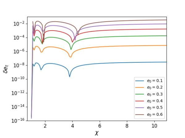
Figure 1: Fractional $e_{t}$ errors, namely $\delta e_{t}=|1-(e_{t}^{PC}/e_{t}^{Num})|$, as a function of $\chi=f/f_{0}$ for three initial $e_{t}$ values at $f_{0}=20\,$Hz. These plots are for a BH binary with $m=20\,M_{\odot}$ as we terminate the $f$ evolution at $f=c^{3}/(G\,m\,\pi\,6^{3/2})$Hz. Clearly, the observed sharp rise in $\delta e_{t}$ values depend critically on $e_{0}$ values and such observations essentially prompted Ref. Moore et al. (2018) argue against the use of PC approach to model eccentric inspirals having $e_{0}>0.2$. Specifically, plots for $e_{0}>0.3$ have $\delta e_{t}>10^{-4}$ and therefore the PC approach should not be used to model such inspirals. Sharp dips in these plots are due to the chance cancellation of $e_{0}^{3}$ terms in the Eq. (20) for $e_{t}$.

II.2 Moore-Robson-Loutrel-Yunes (MoRoLoYu) approach to improve the PC scheme

The new prescription of Ref. Moore et al. (2018) crucially avoids the Taylor expansion of $\omega/\omega_{0}$ expression, given by Eq. (13), for obtaining an analytic expression for $e_{t}$ in terms of $e_{0},\chi$. This is essentially influenced by the fact that the PC scheme does not provide an accurate prescription for the frequency evolution of $e_{t}$ as evident from our Fig. 1 and the associated discussions. Their approach employs the following orbital frequency version of Eq. (13)

$$\frac{F}{F_{0}}= \,\frac{(1-e_{t}^{2})^{3/2}e_{0}^{18/19}(304+121e_{0}^{2})^{1305/2299}}{(1-e_{0}^{2})^{3/2}e_{t}^{18/19}(304+121e_{t}^{2})^{1305/2299}},$$ (21)

where it is natural to define $F_{0}$ and $e_{0}$ using the relation $F(e_{0})=F_{0}$. In practice, $F_{0}$ provides the orbital frequency of a compact binary whose dominant harmonic corresponds to the lower GW frequency cutoff of the detector and $e_{0}$ is the eccentricity of the system at $F_{0}$. We employ numerical inversion of the above expression to obtain the GW frequency evolution of $e_{t}$ after imposing the SPA condition. This ensures that $e_{t}(f)$ prescription should be valid for all allowed $e_{0}$ values, namely $0<e_{0}<1$. We note that certain analytic inversion approaches were provided in Ref. Moore et al. (2018) to avoid numerical inversion. However, we follow the straightforward numerical inversion to ensure no additional approximations are introduced while extracting $e_{t}(f)$ from Eq. (21).

The MoRoLoYu approach provides a different prescription to compute the crucial Fourier phase of Eq. (11) to ensure that it is also valid for $0<e_{0}<1$ cases. This involves providing appropriate expressions for the angular and temporal functions that appear in the definition of $\Psi_{j}$, namely $\Psi_{j}:=j\phi(t^{*}_{j})-2\pi ft^{*}_{j}$, while not employing the PC scheme. It is straightforward to re-write these functions as

$$t-t_{c}= \,\int_{0}^{e_{t}}\frac{de^{\prime}_{t}}{\dot{e_{t}}(e^{\prime}_{t})},$$ (22)

$$\phi-\phi_{c}= \,2\pi\int_{0}^{e_{t}}\frac{F(e^{\prime}_{t})}{\dot{e_{t}}(e^{\prime}_{t})}de^{\prime}_{t}.$$ (23)

To find closed form expressions for these integrals, we need a number of substitutions. First, we replace $F(e_{t})$ in Eq. (23) with our quadrupolar order Eq. (21). The $\dot{e}_{t}$ expression that appears in Eqs. (22) and (23) is replaced by the quadrupolar order $de_{t}/dt$ equation while using Eq. (21) for $F$. These substitutions ensure that the integrands of above two integrals depend only on $e_{t},e_{0}$ and $F_{0}$. This leads to

$$t-t_{c}= \,-\frac{15\,G\,m\,c^{6}}{304\,\eta\,(2\,\pi\,G\,m\,F_{0})^{8/3}\,\sigma(e_{0})^{4}}\,I_{t}(e_{t}),$$ (24)

$$\phi-\phi_{c}= \,-\frac{30\,\pi}{304\,\eta\,(2\,\pi\,G\,m\,F_{0})^{5/3}\,\sigma(e_{0})^{5/2}}\,I_{l}(e_{t}),$$ (25)

where the three new symbols are defined to be

$$\sigma(e_{0})= \,\frac{e_{0}^{12/19}}{1-e_{0}^{2}}\left(1+\frac{121}{304}e_{0}^{2}\right)^{870/2299},$$ (26)

$$I_{t}(e_{t})= \,\frac{19}{48}\,e_{t}^{48/19}F_{1}\left(\frac{24}{19};-\frac{1181}{2299},\frac{3}{2};\frac{43}{19};-\frac{121}{304}e_{t}^{2},e_{t}^{2}\right),$$ (27)

$$I_{l}(e_{t})= \,\frac{19}{30}\,e_{t}^{30/19}{}_{2}F_{1}\left(\frac{124}{2299},\frac{15}{19};\frac{34}{19};-\frac{121}{304}e_{t}^{2}\right),$$ (28)

while $F_{1}$ and ${}_{2}F_{1}$ stand for the ApellF1 hypergeometric function and the generalised hypergeometric function, respectively. We now employ these integrals in the $\Psi_{j}$ equation, given by Eq. (11), and after a few straightforward simplifications obtain

$$\Psi_{j}=j\phi_{c}-2\pi ft_{c}-j\frac{15}{304\,\eta}\left(\frac{c^{3}}{2\,\pi\,G\,m\,F_{0}}\right)^{5/3}\sigma(e_{0})^{-5/2}e_{t}^{30/19}I(e_{t}),$$ (29)

where $I(e_{t})$ is a combination of $I_{t}(e_{t})$ and $I_{l}(e_{t})$ and is given by

$$I(e_{t})= \,\frac{19}{48\left(1+\frac{121e_{t}^{2}}{304}\right)^{124/2299}}\times F_{1}\left(1;-\frac{1181}{2299},\frac{3}{2};\frac{43}{19};\frac{121e_{t}^{2}}{304+121e_{t}^{2}},\frac{e_{t}^{2}}{e_{t}^{2}-1}\right)-\frac{19}{30}{}_{2}F_{1}\left(\frac{124}{2299},\frac{15}{19};\frac{34}{19};-\frac{121e_{t}^{2}}{304}\right).$$ (30)

For our investigations, we followed few additional steps to convert the above $\Psi_{j}(F_{0},e_{0},e_{t})$ expression for obtaining the Fourier-domain phase that should depend on $\Psi_{j}(f,f_{0},e_{0})$. These include first obtaining $e_{t}(F)$ by numerically inverting Eq. (21) at each desired value of frequency $F$ and employing it in Eq. (29) to get $\Psi_{j}$ at that $F$ value. Thereafter, we invoked the stationary phase approximation which demands that the Fourier phase must be computed only at Fourier frequencies which are integral multiples of the orbital frequency $F$. Note that the above approach to obtain $\Psi_{j}(f)$ treats orbital eccentricities in an exact manner and therefore the MoRoLoYu approach is valid for compact binaries of arbitrary bound eccentricities : $0<(e_{0},e_{t})<1$. In our implementation of the approach, we did not employ various fits and approximations suggested in Sec. IV B of Ref. Moore et al. (2018). This is obviously to ensure that an accurate implementation of the NeF model is used for benchmarking our approaches. We would like to state that we Taylor expanded the explicit expressions for $C_{+,\times}^{(j)}$ and $S_{+,\times}^{(j)}$, expressed in terms of Bessel functions of first kind as given by Eqs. (9) in Ref. Moore et al. (2018), while constructing the amplitudes of these templates. However, we did perform several numerical tests to ensure that such expansions in the amplitudes do not affect any of our conclusions. In what follows, we describe a way to obtain analytically quadrupolar order Fourier domain GW response function that should be valid up to moderately high initial eccentricities like $e_{0}\sim 0.6$.

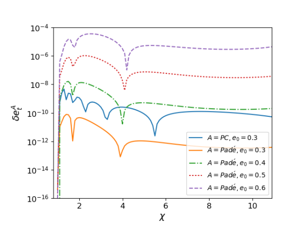
Figure 2: Plots that mainly show fractional errors in $e_{t}$ values while employing our Newtonian Padé approximant for $e_{t}$ and Eq. (21) as a function of $\chi$ for various $e_{0}$ values. We do not display $e_{0}=0.1$ and $0.2$ plots as their Padé based fractional errors are below $10^{-16}$ and essentially represent the rounding errors generated by the computing algorithm. These plots are for $(10\,M_{\odot},10\,M_{\odot})$ BH-BH binary as in Fig. 1. For making easy comparisons, we over plot $\delta e_{t}=|1-(e_{t}^{PC}/e_{t}^{Num})|$ that employs PC scheme based $e_{t}$ expression that includes $\mathcal{O}(e_{0}^{19})$ corrections for the $e_{0}=0.3$ case. It turns out that Padé approximant usually provides two orders of magnitude improvements in these $\delta e_{t}$ estimates compared to their PC counterparts. We find that our Padé approximant is capable of smoothly following the exact quadrupolar order $e_{t}(f)$ evolution for compact binaries even with $e_{0}$ values around $0.6$. Note that it is not computationally expensive to obtain higher order Padé approximant to improve $\delta e_{t}$ estimates for $e_{0}$ values around $0.6$.

II.3 Padé approximation to model quadrupolar order eccentric inspirals

We now explore the possibility of rescuing the PC scheme with the help of an easy and elegant way of resumming a poorly converging power series. Clearly, our PC scheme based analytical $e_{t}(f)$ expression of Sec. II.1 that invoked Taylor expansion does not converge to numerically computed $e_{t}$ values, based on an exact $\omega(e_{t},e_{0},\omega_{0})$ expression. This prompted us to employ the popular Padé approximation, detailed in Ref. Bender and Orszag (1999), for computing the $e_{t}(f)$ and subsequently $\Psi_{j}(f)$ expressions analytically.

It turns out that Padé approximation is helpful for obtaining time-domain inspiral templates for compact binaries in PN-accurate eccentric orbits Tanay et al. (2016). This approximation allowed us to obtain closed form expressions for the hereditary contributions to both GW energy and angular momentum fluxes, which are crucial for computing such templates. Specifically, Padé approximation can be employed to re-sum certain infinite series expressions for the PN-accurate hereditary contributions to GW fluxes from compact binaries in eccentric orbits. Additionally, Padé approximation was invoked to compute GW inspiral template families for quasi-circular inspirals from their Taylor expanded PN counterparts that incorporate higher order PN corrections in terms of the $x$ parameter in Ref. Damour et al. (1998). These template families, referred to as the Padé approximants, were shown to be more effectual and faithful compared to their Taylor expanded PN counterpartsDamour et al. (1998). We note in passing that Padé approximation was employed to model neutron stars and it converges faster to the underlying general relativistic solution than the truncated post-Newtonian ones Gupta et al. (2000).

The simplest form of Padé approximation involves a rational function of two polynomials that provides the original truncated power series under Taylor expansion. Formerly, the simplest Padé approximant to a truncated power series $S_{u}(z)$ in the variable $z$ may be written as

$$P^{m}_{s}(z)= \,\frac{N_{m}(z)}{D_{s}(z)},$$ (31)

where $N_{m}(z)=\sum_{i=0}^{m}n_{i}z^{i}$ and $D_{s}(z)=\sum_{i=0}^{s}d_{i}z^{i}$ are polynomials in $z$ of order $m$ and $s$, respectively. To find the coefficients that define these polynomials, we Taylor expand the approximant $P^{m}_{s}(z)$ upto the same order in $z$ as the original truncated power series $S_{u}(z)$ and then solve the resulting set of linear equations. In other words, if $T_{u}[...]$ denotes the operation of Taylor expanding any function upto an order $u$ of its variable and $S_{u}$ stands for the truncated Taylor series whose Padé approximant we are seeking, we define $P^{m}_{s}$ such that,

$$T_{u}[P^{m}_{s}(z)]= \,S_{u}(z),$$ (32)

where $m+s=u$ is a mandatory condition with $z^{u}$ being the highest order term in the Taylor series required for constructing Padé approximant $P^{m}_{s}(z)$.

It is now straightforward to employ the above detailed Padé approximation on the PC scheme based analytical $e_{t}$ and $\Psi_{j}$ expressions, obtained in Sec. II.1. For the present Padé computations, we have obtained Newtonian accurate $e_{t}(e_{0},\chi)$ and $\Psi_{j}(e_{0},\chi)$ expressions that incorporate $\mathcal{O}(e_{0}^{19})$ and $\mathcal{O}(e_{0}^{20})$ corrections, respectively in the initial orbital eccentricity. This allows us to obtain the following fully analytic Padé approximant for $e_{t}(e_{0},\chi)$ as

$$e_{t}= \,e_{0}\frac{\bar{n}_{0}+\bar{n}_{1}\,z+\bar{n}_{2}\,z^{2}+\bar{n}_{3}\,z^{3}+\bar{n}_{4}\,z^{4}+\bar{n}_{5}\,z^{5}}{1+\bar{d}_{1}\,z+\bar{d}_{2}\,z^{2}+\bar{d}_{3}\,z^{3}+\bar{d}_{4}\,z^{4}},$$ (33)

where $z=e_{0}^{2}$. The coefficients $\bar{n}_{j}$ and $\bar{d}_{k}$, where $j$ runs from $0$ to $5$ while $k$ runs from $1$ to $4$, can easily be computed from the PC scheme based $e_{t}(e_{0},\chi)$ expression that is $\mathcal{O}(e_{0}^{19})$ accurate, as noted earlier. The explicit expressions for all these $10$ coefficients are available in the accompanying Mathematica notebook and we display few of them for the sake of introducing the inherent structure to the readers:

$$\bar{n}_{0}= \,u^{-1/2},$$ (34a)

$$\bar{n}_{1}= \,u^{-3/2}\,\left\{\left(-0.382209+1.86199\,u-3.89605\,u^{2}+4.72722\,u^{3}-3.85449\,u^{4}+2.27674\,u^{5}-0.939021\,u^{6}+0.22659\,u^{7}\right.\right.$$

$$\,-0.0177036\,u^{8}-0.00373226\,u^{9}+0.000682323\,u^{10}-0.0000175432\,u^{11}+5.63003\times 10^{-7}\,u^{12}+3.69953\times 10^{-9}\,u^{13}$$

$$\,\left.-1.1001\times 10^{-11}\,u^{14}-1.0129\times 10^{-15}\,u^{15}\right)/\left(-0.0220143+0.100073\,u-0.192567\,u^{2}+0.213443\,u^{3}-0.161031\,u^{4}\right.$$

$$\,+0.0889986\,u^{5}-0.0323116\,u^{6}+0.00527697\,u^{7}+0.000319898\,u^{8}-0.000193037\,u^{9}+5.35235\times 10^{-6}\,u^{10}$$

$$\,\left.\left.-2.75227\times 10^{-7}\,u^{11}-2.38813\times 10^{-9}\,u^{12}+1.19436\times 10^{-11}\,u^{13}+2.38851\times 10^{-15}\,u^{14}\right)\right\}\,,$$ (34b)

$$\bar{d}_{1}= \,u^{-1}\,\left\{\left(-0.105579+0.521104\,u-1.1073\,u^{2}+1.36672\,u^{3}-1.13418\,u^{4}+0.683062\,u^{5}-0.290007\,u^{6}+0.0737674\,u^{7}\right.\right.$$

$$\,-0.00668361\,u^{8}-0.00116669\,u^{9}+0.000260938\,u^{10}-6.94891\times 10^{-6}\,u^{11}+2.65017\times 10^{-7}\,u^{12}+2.01801\times 10^{-9}\,u^{13}$$

$$\,\left.-8.18895\times 10^{-12}\,u^{14}-1.34108\times 10^{-15}\,u^{15}\right)/\left(-0.00550358+0.0250184\,u-0.0481419\,u^{2}+0.0533608\,u^{3}\right.$$

$$\,-0.0402577\,u^{4}+0.0222497\,u^{5}-0.00807791\,u^{6}+0.00131924\,u^{7}+0.0000799744\,u^{8}-0.0000482594\,u^{9}$$ (34c)

$$\,\left.\left.+1.33809\times 10^{-6}\,u^{10}-6.88068\times 10^{-8}\,u^{11}-5.97032\times 10^{-10}\,u^{12}+2.9859\times 10^{-12}\,u^{13}+5.97128\times 10^{-16}\,u^{14}\right)\right\}\,,$$

$$\bar{d}_{2}= \,u^{-2}\,\left\{\left(-6685.94+35543.3\,u-82569.5\,u^{2}+112439.\,u^{3}-102405.\,u^{4}+66990.1\,u^{5}-31807.1\,u^{6}+10322.2\,u^{7}\right.\right.$$

$$\,-1965.07\,u^{8}+116.15\,u^{9}+26.8824\,u^{10}-4.82738\,u^{11}+0.108707\,u^{12}-0.00375904\,u^{13}-0.0000213561\,u^{14}$$

$$\,\left.+6.78027\times 10^{-8}\,u^{15}+8.25127\times 10^{-12}\,u^{16}\right)/\left(-53.5388+243.379\,u-468.324\,u^{2}+519.094\,u^{3}-391.627\,u^{4}\right.$$

$$\,+216.445\,u^{5}-78.5819\,u^{6}+12.8336\,u^{7}+0.777991\,u^{8}-0.469467\,u^{9}+0.0130169\,u^{10}-0.000669353\,u^{11}$$

$$\,\left.\left.-5.80793\times 10^{-6}\,u^{12}+2.90468\times 10^{-8}\,u^{13}+5.80886\times 10^{-12}\,u^{14}\right)\right\}\,,$$ (34d)

where $u=\chi^{19/9}$. It should be obvious that we restricted our attention to a very specific rational polynomial form. This was essentially the result of many numerical experiments that compared $e_{t}$ values from various Padé approximations against the accurate numerical evaluations of Eq. (21) for $e_{t}$. The above form turned out to be the minimalistic $e_{t}(e_{0},\chi)$ expression that provided fractional relative errors, namely $\delta e_{t}^{Pad\acute{e}}=|1-(e_{t}^{Pad\acute{e}}/e_{t}^{Num})|$, that are $\sim 10^{-5}$ even for $e_{0}\sim 0.6$ cases as evident from Fig. 2. Further, the construction of higher order Padé approximants didn’t necessarily produce fractional errors substantially below the threshold of $10^{-4}$ of Ref. Moore et al. (2018) at moderately high initial eccentricities like $e_{0}\sim 0.6$.

We now present a symbolic Padé approximation based expression for a crucial ingredient to compute frequency domain inspiral templates, namely the Fourier phase $\Psi$ of Eq. (11). The PC ingredient for our computation involves quadrupolar order $\Psi_{j}$ expression that includes $\mathcal{O}(e_{0}^{20})$ corrections in initial eccentricity, as noted earlier. The resulting Padé approximant reads

$$\Psi_{j}= \,j\phi_{c}-2\pi ft_{c}-\frac{3\,j}{256\,\eta\,x^{5/2}}\frac{\hat{n}_{0}+\hat{n}_{1}\,z+\hat{n}_{2}\,z^{2}+\hat{n}_{3}\,z^{3}+\hat{n}_{4}\,z^{4}+\hat{n}_{5}\,z^{5}+\hat{n}_{6}\,z^{6}}{1+\hat{d}_{1}\,z+\hat{d}_{2}\,z^{2}+\hat{d}_{3}\,z^{3}+\hat{d}_{4}\,z^{4}}\,,$$ (35)

where explicit form of these new coefficients $\hat{n}_{j}$ and $\hat{d}_{k}$ are listed in the attached Mathematica notebook. Explicit form for few of these coefficients read

$$\hat{n}_{0}= \,1\,,$$ (36a)

$$\hat{n}_{1}= \,u^{-1}\,\left\{\left(0.00372532-0.0413365\,u+0.208387\,u^{2}-0.634955\,u^{3}+1.31478\,u^{4}-1.97388\,u^{5}+2.22821\,u^{6}-1.89854\,u^{7}\right.\right.$$

$$\,+1.14607\,u^{8}-0.353449\,u^{9}-0.136235\,u^{10}+0.249108\,u^{11}-0.159735\,u^{12}+0.0596684\,u^{13}-0.0133939\,u^{14}$$

$$\,+0.0016679\,u^{15}-0.000101623\,u^{16}+8.60407\times 10^{-6}\,u^{17}-1.7774\times 10^{-6}\,u^{18}+4.74674\times 10^{-8}\,u^{19}$$

$$\,\left.+1.08886\times 10^{-13}\,u^{20}-1.8703\times 10^{-13}\,u^{21}\right)/\left(0.000213461-0.00225419\,u+0.0107362\,u^{2}-0.0306904\,u^{3}\right.$$

$$\,+0.0593036\,u^{4}-0.0828513\,u^{5}+0.086702\,u^{6}-0.067027\,u^{7}+0.0331534\,u^{8}-0.00218905\,u^{9}-0.0125614\,u^{10}$$

$$\,+0.0117481\,u^{11}-0.00561934\,u^{12}+0.00155413\,u^{13}-0.000233167\,u^{14}+0.000015674\,u^{15}-1.06586\times 10^{-6}\,u^{16}$$

$$\,\left.\left.+3.42586\times 10^{-7}\,u^{17}-1.06549\times 10^{-8}\,u^{18}-6.35488\times 10^{-15}\,u^{19}+5.09185\times 10^{-14}\,u^{20}\right)\right\}\,,$$ (36b)

$$\hat{d}_{1}= \,u^{-1}\,\left\{\left(0.00556658-0.0615151\,u+0.308729\,u^{2}-0.936239\,u^{3}+1.92928\,u^{4}-2.88281\,u^{5}+3.23922\,u^{6}-2.74489\,u^{7}\right.\right.$$

$$\,+1.64087\,u^{8}-0.488338\,u^{9}-0.214048\,u^{10}+0.366665\,u^{11}-0.230898\,u^{12}+0.0850503\,u^{13}-0.0188365\,u^{14}$$

$$\,+0.0023162\,u^{15}-0.000141368\,u^{16}+0.0000125252\,u^{17}-2.45494\times 10^{-6}\,u^{18}+6.49348\times 10^{-8}\,u^{19}$$

$$\,\left.+2.61157\times 10^{-13}\,u^{20}-2.55855\times 10^{-13}\,u^{21}\right)/\left(0.000292012-0.00308371\,u+0.0146869\,u^{2}-0.0419841\,u^{3}\right.$$

$$\,+0.0811266\,u^{4}-0.11334\,u^{5}+0.118607\,u^{6}-0.0916922\,u^{7}+0.0453535\,u^{8}-0.0029946\,u^{9}-0.0171838\,u^{10}$$

$$\,+0.0160713\,u^{11}-0.0076872\,u^{12}+0.00212603\,u^{13}-0.000318971\,u^{14}+0.0000214419\,u^{15}-1.45808\times 10^{-6}\,u^{16}$$

$$\,\left.\left.+4.68655\times 10^{-7}\,u^{17}-1.45759\times 10^{-8}\,u^{18}-8.69341\times 10^{-15}\,u^{19}+6.96559\times 10^{-14}\,u^{20}\right)\right\}\,,$$ (36c)

$$\hat{d}_{2}= \,u^{-2}\left\{\left(0.00334745-0.0387328\,u+0.204895\,u^{2}-0.659079\,u^{3}+1.44779\,u^{4}-2.31304\,u^{5}+2.78762\,u^{6}-2.56801\,u^{7}\right.\right.$$

$$\,+1.76572\,u^{8}-0.804281\,u^{9}+0.104142\,u^{10}+0.179923\,u^{11}-0.174374\,u^{12}+0.0859044\,u^{13}-0.0262981\,u^{14}$$

$$\,+0.00499171\,u^{15}-0.0005403\,u^{16}+0.0000300179\,u^{17}-2.25185\times 10^{-6}\,u^{18}+4.10531\times 10^{-7}\,u^{19}$$

$$\,\left.-9.86595\times 10^{-9}\,u^{20}-5.54463\times 10^{-15}\,u^{21}+3.18323\times 10^{-14}\,u^{22}\right)/\left(0.0000266315-0.000281234\,u\right.$$

$$\,+0.00133945\,u^{2}-0.00382895\,u^{3}+0.00739875\,u^{4}-0.0103366\,u^{5}+0.010817\,u^{6}-0.00836233\,u^{7}+0.00413624\,u^{8}$$

$$\,-0.000273108\,u^{9}-0.00156716\,u^{10}+0.0014657\,u^{11}-0.000701072\,u^{12}+0.000193894\,u^{13}-0.0000290901\,u^{14}$$

$$\,+1.9555\times 10^{-6}\,u^{15}-1.32977\times 10^{-7}\,u^{16}+4.27413\times 10^{-8}\,u^{17}-1.32932\times 10^{-9}\,u^{18}-7.92839\times 10^{-16}\,u^{19}$$

$$\,\left.\left.+6.35262\times 10^{-15}\,u^{20}\right)\right\}\,.$$ (36d)

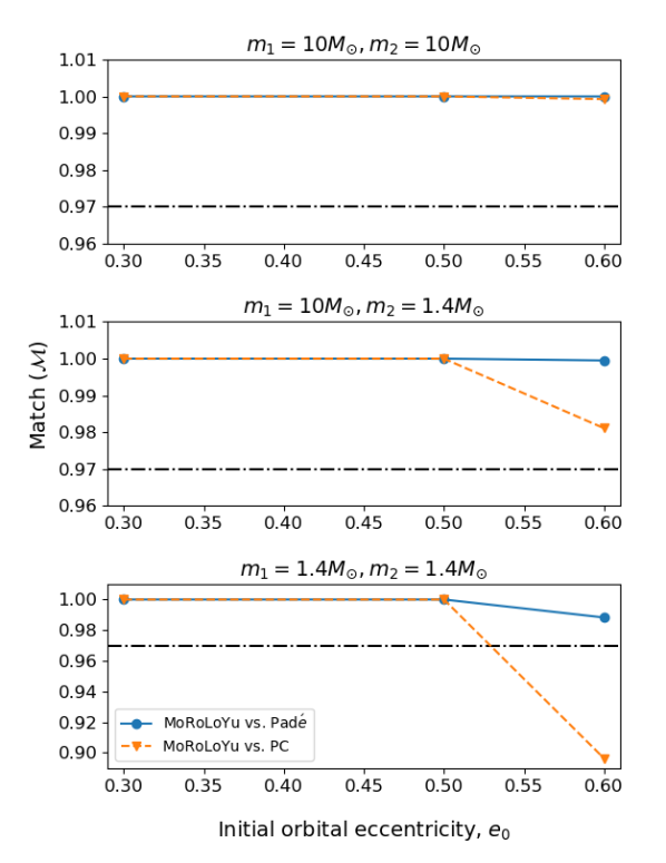
Figure 3: Match ($\mathcal{M}$) plots for the three traditional LIGO relevant compact binaries having eccentricities up to $0.6$ at a GW frequency of $20$Hz. We let the expected eccentric GW signal to be described by the MoRoLoYu approach, described in Sec. II.2, while our Padé approximant provided the fully analytic eccentric inspiral templates. The dashed line marks the $0.97$ $\mathcal{M}$ value and it is evident that our quadrupolar order Padé approximant templates are both effectual and faithful to our expected GW signal from data analysis considerations. The associated PC based templates show drop in match estimates around $e_{0}\sim 0.5$. We have computed such computationally expensive $\mathcal{M}$ estimates at intermediate $e_{0}$ values randomly to ensure that these few point plots are representatives of a finely sampled $e_{0}$ match plots.

We are now in a position to compare our Padé approximant $\tilde{h}(f)$ with the ones arising from our implementation of the MoRoLoYu and PC approaches. This is pursued with the help of $\mathcal{M}$ estimates. Recall that the $\mathcal{M}(h_{s},h_{t})$ estimates provide certain effectualness and faithfulness criteria between the members of two GW waveform families denoted here as $h_{s}$ and $h_{t}$ Damour et al. (1998). A template family $h_{t}$ is said to be effectual in detection and faithful for parameter estimation if it produces a match $\mathcal{M}\geq 0.97$ with a signal waveform $h_{s}$. An effectual template is desirable to ensure detection of more than $90\%$ of expected GW signals while a faithful template is mandatory to infer the signal parameters with smaller biases. Following Ref. Damour et al. (1998), we define

$$\mathcal{M}= \,\max_{t_{c},\phi_{c}}\frac{(h_{s}|h_{t})}{\sqrt{(h_{s}|h_{s})(h_{t}|h_{t})}},$$ (37)

where the inner product $(a|b)$ is given as,

$$(a|b)= \,4\,Re\int_{f_{l}}^{f_{u}}\frac{\tilde{a}^{*}(f)\tilde{b}(f)}{S_{n}(f)}df.$$ (38)

In practice, $h_{s}$ and $h_{t}$ may be treated as the members of the expected GW signal and its approximate template families. Further, $S_{n}(f)$ stands for the one-sided noise spectral density of a GW detector and we use the zero-detuned high power (ZDHP) noise configuration of the Advanced LIGO at design sensitivity Harry and LIGO Scientific Collaboration (2010). The limits of the above integral provide certain lower and upper cut-off frequencies and we let $f_{l}=20$Hz. For the present studies, we choose $f_{u}$ to be the popular GW frequency associated with the last stable circular orbit of a test particle in the Schwarzschild metric, namely $f_{u}=c^{3}/(Gm\pi 6^{3/2})$. Additionally, we have explored the effect of orbital eccentricity on the above $f_{u}$ estimate with the help of Eqs. (D1) and (D2) of Ref. Yunes et al. (2009). The fact that orbital eccentricities were $\sim 10^{-2}$ at GW frequencies around $200$Hz even for our $e_{0}\sim 0.6$ systems justified the use of above expression for $f_{u}$ in our numerical experiments. Additionally, we have explicitly verified that use of the above mentioned eccentric $f_{u}$ didn’t affect our match estimates in high $e_{0}$ systems in any noticeably manner. In Fig. 3, we plot the $\mathcal{M}$-estimates for the three traditional compact binary systems having various values of initial orbital eccentricities. The traditional binaries include $1.4\,M_{\odot}-1.4\,M_{\odot}$ NS binaries, $10\,M_{\odot}-10\,M_{\odot}$ BH binaries and their mixtures. We let $\tilde{h}(f)$ that arise from the MoRoLoYu approach to be the expected eccentric inspiral signal as detailed in Sec. II.2. The templates are provided by our Padé approximant that employs Eq. (35) for $\Psi_{j}$. Further, we keep various amplitudes at the quadrupolar order and employ Padé approximation based expression for $e_{t}(f)$ (Eq. (33)) in both waveform families for the ease of implementation. The use of quadrupolar order amplitudes is justifiable as match estimates crucially depend on the Fourier phase evolution differences and not on the amplitudes of underlying waveform families. Further, we usually included the first $22$ harmonics while pursuing our match computations. We have verified in many instances that the results were not sensitive to the number of harmonics used by substantially increasing their numbers.

Plots in Fig. 3 reveal that Padé approximant is capable of providing $\mathcal{M}$ estimates that are $\geq 0.97$ even for $e_{0}$ values in the neighborhood of $0.6$. This allows us to state that our quadrupolar order Padé approximant should be both effectual and faithful to model inspiral GWs from compact binaries with moderately high initial eccentricities Damour et al. (1998). In contrast, our numerical experiments show that the PC scheme based templates provide substantially lower $\mathcal{M}$ estimates especially for compact binaries that contain neutron stars. We now detail how to obtain 1PN extensions of these three approaches and their implications.

III Extending Eccentric Fourier-domain families to PN orders

We begin by summarizing how one extends the PC scheme to 1PN order, as detailed in Ref. Tanay et al. (2016). This is followed by a brief summary of our detailed computations that essentially extend the MoRoLoYu approach to 1PN order. Such a computation allows us to explore if the deficiencies of the PC scheme, evident at the quadrupolar order, persists even at the PN orders. This is followed by a straightforward extension of our quadrupolar order Padé approximant to 1PN order while keeping the amplitudes to the Newtonian order and exploration of its $\mathcal{M}$ estimate implications. Finally, we list subtleties of extending our Padé approximant to higher PN orders, influenced by Ref. Moore and Yunes (2019).

III.1 1PN extension of the post-circular approximation

We begin by describing how to compute an ingredient that is critical to extend the quadrupolar order PC scheme to 1PN order, namely 1PN accurate analytic $e_{t}$ expression with the leading order $e_{0}$ corrections. This requires us to compute 1PN-accurate expression for $d\omega/de_{t}$ by dividing 1PN-accurate expressions for $d\omega/dt$ and $de_{t}/dt$, given by Eqs. (3.12) of Ref. Tanay et al. (2016). This leads to

$$d\omega/de_{t}=\biggl{\{}-\frac{18}{19e_{t}}-\frac{3}{10108e_{t}}\left(-2833+5516\eta\right)\left(\frac{Gm\omega}{c^{3}}\right)^{2/3}\biggr{\}}\,\omega\,,$$ (39)

where we have restricted our attention to the leading order $e_{t}$ contributions. We now replace $\omega$ that appears in the PN expansion parameter by its Newtonian version, namely $\omega=\omega_{0}\,\left(e_{0}/e_{t}\right)^{18/19}$. The resulting equation may be written as

$$d\omega/\omega\sim\left\{-\frac{18}{19e_{t}}-\frac{3}{10108}\left(\frac{e_{0}^{12/19}}{e_{t}^{31/19}}\right)\left(-2833+5516\eta\right)\,x_{0}\right\}de_{t}\,,$$ (40)

where $x_{0}=\left(G\,m\,\omega_{0}/c^{3}\right)^{2/3}$. The above equation can be integrated to get $\ln(\omega/\omega_{0})$ as a function of $\omega_{0},e_{t}$ and $e_{0}$. The exponential of such an expression, followed by a bivariate expansion in $e_{t}$ and $x_{0}$ results in

$$\omega \sim\left\{\left(\frac{e_{0}}{e_{t}}\right)^{18/19}+x_{0}\left(\frac{2833-5516}{2128}\eta\right)\left[\left(\frac{e_{0}}{e_{t}}\right)^{18/19}-\left(\frac{e_{0}}{e_{t}}\right)^{30/19}\right]\right\}\omega_{0}\,.$$ (41)

It should be obvious that we need to assume $x_{0}\ll 1$ and $e_{t}\ll 1$ during such a bivariate expansion and therefore we are implementing a PN-accurate version of the quadrupolar order PC scheme. Explicit 1PN-accurate $e_{t}$ expression is obtained by first replacing $e_{t}$ terms that appear in the coefficients of the $x_{0}$ terms by its Newtonian accurate expression, namely $e_{t}=e_{0}\,\chi^{-19/18}$. The resulting intermediate expression is inverted assuming $x_{0}\ll 1$ and $e_{0}\ll 1$ which leads to

$$e_{t}\sim e_{0}\left\{\chi^{-19/18}+x_{0}\left(\frac{2833}{2016}-\frac{197}{72}\eta\right)\left(-\chi^{-7/18}+\chi^{-19/18}\right)\right\}\,.$$ (42)

We now re-write the above expression for $e_{t}$ in terms of usual PN parameter $x$ by noting that $x_{0}=x\,\chi^{-2/3}$. The resulting 1PN-accurate $e_{t}(e_{0},x,\chi)$ that includes $\mathcal{O}(e_{0})$ corrections reads

$$e_{t}\sim e_{0}\left\{\chi^{-19/18}+x\left(\frac{2833}{2016}-\frac{197}{72}\eta\right)\left(-\chi^{-19/18}+\chi^{-31/18}\right)\right\}.$$ (43)

It is fairly straightforward to repeat the computations of Sec. II.1 to obtain $\Psi_{j}$ that incorporates $\mathcal{O}(e_{0}^{2})$ eccentricity corrections with the help of Eq. (17) even at 1PN order, as detailed in Ref. Tanay et al. (2016). The final result is

$$\Psi_{j}\sim j\phi_{c}-2\pi ft_{c}-\left(\frac{3j}{256\eta\,x^{5/2}}\right)\left\{1-\frac{2355e_{0}^{2}}{1462}\chi^{-19/9}+x\left[\frac{3715}{756}+\frac{55}{9}\eta+\left(\left[-\frac{2045665}{348096}-\frac{128365}{12432}\eta\right]\chi^{-19/9}\right.\right.\right.$$

$$\qquad\left.\left.\left.{}+\left[-\frac{2223905}{491232}+\frac{154645}{17544}\eta\right]\chi^{-25/9}\right)e_{0}^{2}\right]\right\}\,,$$ (44)

where $x=(\frac{G\,m\,2\,\pi\,F}{c^{3}})^{2/3}$ and $\chi=F/F_{0}$ have to be evaluated at the stationary points i.e. at $F=f/j$ and $F_{0}=f_{0}/j$ with $j$ being the harmonic index.

It is straightforward but demanding to extend these calculations to include higher order $e_{0}$ corrections. In fact, we have computed 1PN-accurate expressions for $e_{t}$ and $\Psi$ upto $\mathcal{O}(e_{0}^{19})$ and $\mathcal{O}(e_{0}^{20})$, respectively. The resulting 1PN-accurate PC scheme based $\tilde{h}(f)$ with quadrupolar order amplitudes will be used to explore the suitability of employing the PC scheme at 1PN order for eccentric inspirals. The other ingredient, namely 1PN extension of the MoRoLoYu approach will be discussed in the next subsection.

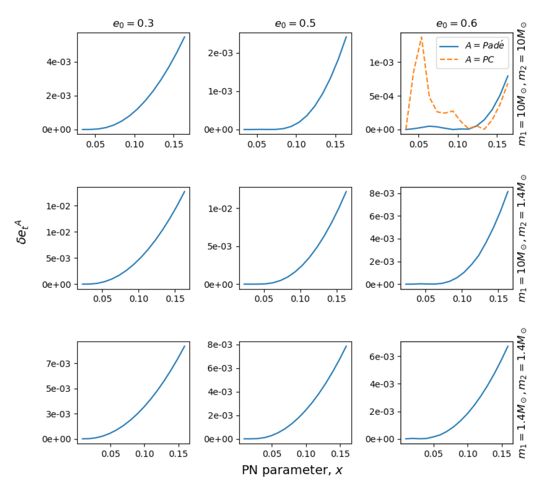
Figure 4: Fractional errors in 1PN accurate $e_{t}$ values as a function of the dimensionless $x$ parameter. The associated $e_{t}$ values are obtained by i) numerically inverting Eq. (49) for $x(e_{t},e_{0},x_{0})$ and ii) by using our Eq. (III.3) for the 1PN-accurate $e_{t}^{Pad\acute{e}}$. We restrict our attention to the traditional LIGO binaries with three initial eccentricities of $0.3,0.5$ and $0.6$. In contrast to Fig. 2 plots, these fractional error plots depend on intrinsic compact binary parameters like $m$ and $\eta$ and they begin at $(G\,m\,20\,\pi/c^{3})^{2/3}$ and end at $x=1/6$. Sharp rise in $\delta e_{t}$ at higher $x$ values, visible in all plots, may be attributed to the different ways PN corrections are included in our analytic and numerical approaches to obtain $e_{t}$ values. Additionally, our numerical experiments show similar behaviour for $\delta e_{t}$ plots that employ 1PN-accurate PC scheme based expression for $e_{t}$ as showed in the dashed plot of top right panel. Further, PC based $e_{t}$ values suffer from system dependent sharp variations in $\delta e_{t}$ values.

III.2 1PN accurate $e_{t}$ and $\Psi$ in our MoRoLoYu approach

This subsection sketches a way to obtain 1PN accurate expressions for $e_{t}$ and $\Psi$ that are exact in $e_{0}$, influenced by ideas gathered from Refs. Mikóczi et al. (2012); Moore and Yunes (2019). This extension allows us to benchmark both our fully analytic 1PN accurate PC scheme and its Padé approximation to model frequency domain GW templates for eccentric inspirals. We begin by extending our quadrupolar order $\omega(\omega_{0},e_{0},e_{t})$ expression, given by Eq. (41), to 1PN order.

For practical reasons, we plan to compute 1PN-accurate $x(e_{t},e_{0},x_{0})$ expression and the starting point of these computations involves 1PN-accurate equations for $\dot{x}$ and $\dot{e_{t}}$, extracted from Eqs. (3.12a),(3.12b),(B9a - B9d) in Ref. Tanay et al. (2016). It is straightforward to obtain 1PN-accurate expression for $dx/de_{t}=\dot{x}/\dot{e_{t}}$ and it reads

$$\frac{dx}{de_{t}}= \,x\left[-\frac{2\,(96+292e_{t}^{2}+37e_{t}^{4})}{e_{t}\,(1-e_{t}^{2})\,(304+121e_{t}^{2})}-\frac{x}{42\,e_{t}\,(1-e_{t}^{2})(304+121e_{t}^{2})^{2}}\left(-2175744+4236288\,\eta\right.\right.$$ (45)

$$\,\left.\left.+e_{t}^{2}(11073288-6573728\eta)+e_{t}^{4}(-4607952+3626672\eta)+e_{t}^{6}(192543-219632\eta)\right)\right].$$

Thereafter, we write the above equation symbolically as

$$\frac{dx}{de_{t}}= \,x\left[a_{0}(e_{t})+a_{1}(e_{t})\,x\right]\,.$$ (46)

We seek its 1PN-accurate solution in the form

$$x(e_{t})= \,x_{0}\left[b_{0}(e_{t})+b_{1}(e_{t})\,x_{0}\right],$$ (47)

where $x_{0}=(\frac{Gm2\pi F_{0}}{c^{3}})^{2/3}$ and $b_{0}$, $b_{1}$ are certain functions of $e_{0}$ and $e_{t}$. The explicit expressions for these functions are obtained by inserting Eq. (47) into Eq.(46) and expanding the resulting equation while incorporating all contributions accurate to $x_{0}^{2}$. This leads to a set of coupled ordinary differential equations for the unknown coefficient functions $b_{0}(e_{t})$ and $b_{1}(e_{t})$ and these equations may be written as

$$b_{0}^{\prime}(e_{t})= \,a_{0}b_{0},$$ (48a)

$$b_{1}^{\prime}(e_{t})= \,a_{0}b_{1}+a_{1}b_{0}^{2}\,,$$ (48b)

where primes (^′) denote differentiation w.r.t $e_{t}$. It is natural to impose the following constraints like $b_{0}(e_{0})=1$ and $b_{1}(e_{0})=0$, mainly to ensure that $x(e_{0})=x_{0}$. This allows us to obtain a 1PN-accurate expression for $x(e_{t})$:

$$x(e_{t},e_{0},x_{0})= \,x_{0}\left\{\left(\frac{1-e_{t}^{2}}{1-e_{0}^{2}}\right)\left(\frac{e_{0}}{e_{t}}\right)^{12/19}\left(\frac{304+121e_{0}^{2}}{304+121e_{t}^{2}}\right)^{870/2299}+x_{0}\frac{(1-e_{t}^{2})\,e_{0}^{12/19}(304+121e_{0}^{2})^{1740/2299}}{16056942720\,(1-e_{0}^{2})^{2}\,e_{t}^{12/19}(304+121e_{t}^{2})^{870/2299}}\right.$$ (49)

$$\,\left.\left[\left(\frac{e_{0}}{e_{t}}\right)^{12/19}\mathcal{G}(e_{t})-\mathcal{G}(e_{0})\right]\right\}\,,$$

where

$$\mathcal{G}(e)= \,\frac{52}{(304+121e^{2})^{3169/2299}}\left[29408320\,(-2833+5516\eta)+168\,e^{2}(-1555687953+1605256000\eta)\right.$$

$$\,\left.+e^{4}(-4472255861+16145243380\eta)\right]+2^{1118/2299}19^{1429/2299}e^{2}(-37041343+14343420\eta)$$

$$\,{}_{2}F_{1}\left(\frac{870}{2299},\frac{13}{19};\frac{32}{19};-\frac{121}{304}e^{2}\right).$$

The above expression provides certain 1PN-accurate solution to Eq. (45) while the ${}_{2}F_{1}(...)$ in the $\mathcal{G}(e)$ expression stands for the computationally demanding - generalised Hypergeometric function.

We note that the present approach can, in principle, be extended to higher PN orders, provided closed form expressions exist for higher PN order contributions to $\dot{x}$ and $\dot{e_{t}}$. In other words, it will be difficult to extend the approach when we deal with hereditary contributions to GW fluxes that do not support closed form expressions Rieth and Schäfer (1997).

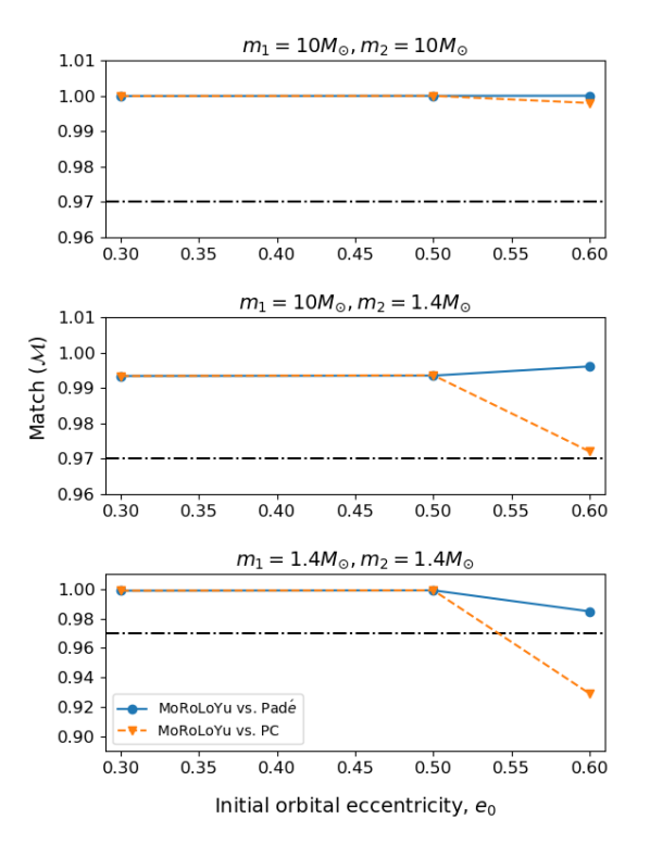
Figure 5: Plots of $\mathcal{M}$-values as a function of $e_{0}$ for the traditional binaries entering the aLIGO frequency window and other specifications are similar to those in Fig. 3. We let the expected inspiral GW signal to be modeled by our 1PN-accurate version of the MoRoLoYu approach while the templates belong to our 1PN-accurate $\tilde{h}^{Pad\acute{e}}$ waveform family. We find that our Padé templates are fairly faithful to the GW signals that treat eccentricity in an exact manner up to $e_{0}\sim 0.6$ while the associated PC templates suffer drop in match numbers around $e_{0}\sim 0.5$.

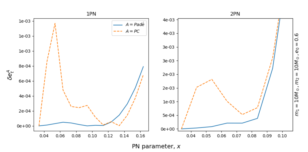
Figure 6: Plots of fractional relative errors in $e_{t}$ at first and second post-Newtonian orders as a function of $x$ for a BBH system with $e_{0}=0.6$. The orange plot in the left panel employs 1PN accurate PC scheme based $e_{t}$ values, obtained by an extension of Eq. (43) that included $\mathcal{O}(e_{0}^{19})$ corrections at each PN order and its Padé counterpart, the blue curve, employed Eq. (III.3). The right panel plots employ the 2PN-accurate extensions of both PC and Padé approaches for computing analytic $e_{t}$ expressions. Additionally, the numerical $e_{t}$ values that are required to compute these $\delta e_{t}^{A}=|1-(e_{t}^{A}/e_{t}^{Num})|$ plots employ our 1PN-accurate Eq. (49) that provides 1PN extension of the MoRoLoYu approach. For the right panel plots, we numerically solve Eq. (56b) to estimate $e_{t}^{Num}$ values. These plots reveal that Padé based $e_{t}$ values appear to smooth out the peculiarities in the fractional errors coming from the PC scheme based $e_{t}$ values at both 1PN and 2PN orders. However, the rapidly growing fractional errors with the PN expansion parameter suggests that a Padé-ing on $x$ might also be required to precisely model $e_{t}(f)$. This is mainly because our numerical experiments indicate that the sharp variations in $\delta e_{t}^{A}$ during the later part of the inspiral are rather independent of $e_{0}$ values and nature of the compact binaries, as evident from various subplots in our Fig. 4.

We compute 1PN-accurate Fourier phase $\Psi$ of the MoRoLoYu approach by obtaining 1PN-accurate versions of the time and orbital phase evolution functions, namely Eq. (22) and (23). This requires us to employ 1PN-accurate version of $\dot{e_{t}}(e_{t}^{\prime})$ in both these integrals and we use

$$\frac{de_{t}}{dt}= \,-\frac{c^{3}x^{4}\eta e_{t}}{Gm\left(1-e_{t}^{2}\right)^{5/2}}\left\{\frac{304+121e_{t}^{2}}{15}+\frac{x\left(-67608-228704\eta+e_{t}^{2}(718008-651252\eta)+e_{t}^{4}(125361-93184\eta)\right)}{2520\left(1-e_{t}^{2}\right)}\right\}.$$ (50)

The above expression is identical to Eq. (3.12b) in Ref. Tanay et al. (2016) and we need to use $F=c^{3}\,x^{3/2}/(G\,m\,2\,\pi)$ in Eq. (23) for $\phi$ to be consistent. Thereafter, we employ our 1PN-accurate expression for $x(e_{t},e_{0},x_{0})$, given by Eq. (49), in these two integrals and this allows us to express their integrands in terms of $x_{0},e_{t},e_{0}$. Next step involves expansion of these integrands in terms of $x_{0}$ up to 1PN order but the resulting $t$ and $\phi$ integrals still remain non-trivial to evaluate analytically due to complex dependence on the variable $e_{t}^{\prime}$. We perform these integrations by first expanding coefficient of each $x_{0}$ term in terms of $e_{t}$ without expanding the $e_{0}$ terms and this is influenced by Ref. Moore and Yunes (2019). In our computations, we keep $e_{t}$ contributions accurate to $\mathcal{O}(e_{t}^{40})$ and this is again influenced by the detailed analysis provided in Sec. (5.1),(5.2) of Moore and Yunes (2019). The integration of resulting expressions with respect to $e_{t}$ provided us with 1PN-accurate time and phase functions. We list below expressions for these time and phase functions that incorporate only the leading order corrections in $e_{t}$ as Eqs. (III.2) and (III.2), respectively. It is important to note that $e_{0}$ contributions are treated in an exact manner in these two expressions. A few comments are in order. The 1PN-accurate expressions for time and phase functions which treat both $e_{0}$ and $e_{t}$ in an exact manner using Hypergeometric functions, were first provided by Eq. (59) of Ref. Mikóczi et al. (2015a). We have verified that our Eqs. (51) and (52) are in agreement with the $t$ and $\phi$ expressions of Ref. [61], given by their Eq. (59), when Taylor expanding relevant expressions around $e_{t}=0$ while not expanding in $e_{0}$. We now can obtain with the help of these 1PN-accurate expressions a 1PN-accurate version of $\Psi$ as $\Psi_{j}:=j\phi(t^{*}_{j})-2\pi ft^{*}_{j}$. The fact that we have treated the initial eccentricity in an exact manner in our 1PN accurate $\Psi_{j}$ expression makes it suitable to model eccentric inspirals with moderately high initial eccentricities.

$$t-t_{c}= \,-\frac{95\times 19^{1181/2299}\left(1-e_{0}^{2}\right)^{4}e_{t}^{48/19}Gm}{2\times 2^{2173/2299}e_{0}^{48/19}\left(304+121e_{0}^{2}\right)^{3480/2299}c^{3}\,x_{0}^{4}\,\eta}-\frac{25\times 19^{311/2299}\left(1-e_{0}^{2}\right)^{3}(889-444\eta)\,e_{t}^{36/19}Gm}{288\times 2^{1055/2299}e_{0}^{36/19}\left(304+121e_{0}^{2}\right)^{2610/2299}c^{3}\,x_{0}^{3}\,\eta}$$

$$\,\bigg{\{}1-\frac{10334784\times 2^{1181/2299}19^{870/2299}e_{t}^{12/19}}{35\,e_{0}^{12/19}\left(304+121e_{0}^{2}\right)^{3169/2299}(889-444\eta)}\bigg{[}1-\frac{5516\eta}{2833}+e_{0}^{2}\left(\frac{32669447013}{10414221320}-\frac{842759400\eta}{260355533}\right)$$

$$\,+e_{0}^{4}\left(\frac{4472255861}{83313770560}-\frac{807262169\eta}{4165688528}\right)+\frac{19^{1429/2299}\left(304+121e_{0}^{2}\right)^{870/2299}}{2^{1181/2299}}\bigg{(}e_{0}^{2}\left(\frac{703785517}{135384877160}-\frac{1048173\eta}{520711066}\right)$$

$$\,+e_{0}^{4}\left(\frac{4482002503}{2166158034560}-\frac{6675207\eta}{8331377056}\right)\bigg{)}{}_{2}F_{1}\left(\frac{870}{2299},\frac{13}{19};\frac{32}{19};-\frac{121}{304}e_{0}^{2}\right)\bigg{]}\bigg{\}}\,,$$ (51)

$$\phi-\phi_{c}= \,-\frac{19^{2175/2299}\left(1-e_{0}^{2}\right)^{5/2}e_{t}^{30/19}}{2^{2795/2299}e_{0}^{30/19}\left(304+121e_{0}^{2}\right)^{2175/2299}x_{0}^{5/2}\eta}-\frac{e_{t}^{18/19}\left(1-e_{0}^{2}\right)^{3/2}(14135+630\eta)}{504\times 2^{1677/2299}19^{994/2299}e_{0}^{18/19}\left(304+121e_{0}^{2}\right)^{1305/2299}x_{0}^{3/2}\eta}$$

$$\,\bigg{\{}1-\frac{645924\times 2^{1181/2299}19^{870/2299}e_{t}^{12/19}}{e_{0}^{12/19}\left(304+121e_{0}^{2}\right)^{3169/2299}(2827+126\eta)}\bigg{[}1-\frac{5516\eta}{2833}+e_{0}^{2}\left(\frac{32669447013}{10414221320}-\frac{842759400\eta}{260355533}\right)$$

$$\,+e_{0}^{4}\left(\frac{4472255861}{83313770560}-\frac{807262169\eta}{4165688528}\right)+\frac{19^{1429/2299}(304+121e_{0}^{2})^{870/2299}}{2^{1181/2299}}\bigg{(}e_{0}^{2}\left(\frac{703785517}{135384877160}-\frac{1048173\eta}{520711066}\right)$$

$$\,+e_{0}^{4}\left(\frac{4482002503}{2166158034560}-\frac{6675207\eta}{8331377056}\right)\bigg{)}{}_{2}F_{1}\left(\frac{870}{2299},\frac{13}{19};\frac{32}{19};-\frac{121}{304}e_{0}^{2}\right)\bigg{]}\bigg{\}}\,.$$ (52)

However, few more steps are required to fully operationalize the above computed PN-accurate $\Psi(x_{0},e_{t},e_{0})$ expression. First, one needs to numerically invert our 1PN-accurate expression for $x(x_{0},e_{t},e_{0})$, namely Eq. (49), for extracting $e_{t}(x,x_{0},e_{0})$ that leads to a chart between $e_{t}$ and $F$ values. Thereafter, the stationary phase condition should be invoked to replace $F$ and $F_{0}$ by their Fourier frequency counterparts $f/j$ and $f_{0}/j$, respectively. We refrain from showing the lengthy expression for the resulting 1PN-accurate $\Psi_{j}$ that extends its Newtonian counterpart. It is obvious that the resulting ready-to-use template family will be computationally expensive due to presence of these special functions and numerical treatments. In the next subsection, we outline steps to obtain 1PN-accurate Padé approximants that provide fully analytic $e_{t}$ and $\Psi$ expressions.

III.3 Our 1PN-accurate $e_{t}$ and $\Psi$ using Padé approximants

We provide here a brief description for computing 1PN-accurate fully analytic Padé approximant associated with our 1PN-accurate PC scheme based $\tilde{h}(f)$, detailed in Sec. III.1. Clearly, this is pursued to probe the ability of such an approximant to model eccentric inspirals in comparison with our 1PN-accurate extension of the MoRoLoYu approach that treats $e_{0}$ effects in an exact manner. Our Padé approximant, as expected, requires PC scheme based expressions for $e_{t}$ and $\Psi_{j}$ and we specifically employ such 1PN accurate $e_{t}$ and $\Psi_{j}$ expressions that incorporate $\mathcal{O}(e_{0}^{19})$ and $\mathcal{O}(e_{0}^{20})$ corrections in initial eccentricity. We obtain Padé approximations of these quantities by applying the resummation technique individually to Newtonian and 1PN contributions. This allows us to propose the following expression to obtain a simplistic 1PN-accurate Padé approximation for $e_{t}$

$$e_{t}= \,e_{0}\bigg{\{}\frac{\bar{n}_{0}+\bar{n}_{1}\,z+\bar{n}_{2}\,z^{2}+\bar{n}_{3}\,z^{3}+\bar{n}_{4}\,z^{4}+\bar{n}_{5}\,z^{5}}{1+\bar{d}_{1}\,z+\bar{d}_{2}\,z^{2}+\bar{d}_{3}\,z^{3}+\bar{d}_{4}\,z^{4}}+x\,\frac{\bar{n}^{\prime}_{0}+\bar{n}^{\prime}_{1}\,z+\bar{n}^{\prime}_{2}\,z^{2}+\bar{n}^{\prime}_{3}\,z^{3}+\bar{n}^{\prime}_{4}\,z^{4}+\bar{n}^{\prime}_{5}\,z^{5}}{1+\bar{d}^{\prime}_{1}\,z+\bar{d}^{\prime}_{2}\,z^{2}+\bar{d}^{\prime}_{3}\,z^{3}+\bar{d}^{\prime}_{4}\,z^{4}}\bigg{\}}\,.$$

For the sake of simplicity, we denote 1PN order coefficients with the help of ^′ symbols. These coefficients can be obtained from their 1PN order counterparts, present in our 1PN accurate PC scheme based $e_{t}$ expression. Further, the Newtonian order coefficients like $\bar{n}_{0}...\bar{n}_{5}$, $\bar{d}_{1}...\bar{d}_{4}$ are identical to those present in Eq. (33). The resulting expression allows us to compute the fractional differences between $e_{t}$ values that are based on our 1PN-accurate extension of the MoRoLoYu and Padé approximations for $e_{t}$. These differences are expected to depend on both total mass and mass ratio as Eq. (41) for 1PN-accurate $\omega$ depends on these quantities. In Fig. 4, we plot fractional errors in $e_{t}$ as a function of the PN expansion parameter $x$. We find that $\delta e_{t}$ values are essentially independent of $e_{0}$ values and sharp rises in $\delta e_{t}$ values are observed when $x$ values cross $0.1$. This may be attributable to the differences in the way PN corrections are incorporated in Eqs. (49) and (III.3). We found similar behaviour for 1PN-accurate fractional errors up to $e_{0}=0.6$, for systems having $m<50\,M_{\odot}$. The curves follow similar pattern up to mild eccentricities $e_{0}\sim 0.3$ for systems with $m>50\,M_{\odot}$. However, more heavier systems with $m>50\,M_{\odot}$ and with $e_{0}>0.3$ do not display similar increases in fractional errors with the PN expansion parameter, $x$. This is expected as such systems will evolve rapidly from $f_{0}=20$ Hz to the ISCO frequency without causing any noticeable disagreement between our Padé approximant for $e_{t}$ and its numerical counterpart. Further, our numerical experiments reveal that $\delta e_{t}$ plots created with the PC scheme based 1PN-accurate $e_{t}$ expression show similar $x$ variations though these plots are spikey at higher $e_{0}$ values. These considerations suggest that multi-Padé expression that perform Padé-ing on both $x$ and $e_{0}$ values may be required while constructing PN extensions of Eq. (III.3). This issue requires further investigations. We proceed to list our 1PN accurate Padé approximated Fourier phases expression, computed from the 1PN-accurate PC scheme based $\Psi_{j}$ expression that includes $\mathcal{O}(e_{0}^{20})$ order corrections in $e_{0}$. The symbolic expression for $\Psi_{j}$ reads

$$\Psi_{j}= \,j\phi_{c}-2\pi ft_{c}-\frac{3\,j}{256\,\eta\,x^{5/2}}\bigg{\{}\frac{\hat{n}_{0}+\hat{n}_{1}\,z+\hat{n}_{2}\,z^{2}+\hat{n}_{3}\,z^{3}+\hat{n}_{4}\,z^{4}+\hat{n}_{5}\,z^{5}+\hat{n}_{6}\,z^{6}}{1+\hat{d}_{1}\,z+\hat{d}_{2}\,z^{2}+\hat{d}_{3}\,z^{3}+\hat{d}_{4}\,z^{4}}$$

$$+x\,\frac{\hat{n}^{\prime}_{0}+\hat{n}^{\prime}_{1}\,z+\hat{n}^{\prime}_{2}\,z^{2}+\hat{n}^{\prime}_{3}\,z^{3}+\hat{n}^{\prime}_{4}\,z^{4}+\hat{n}^{\prime}_{5}\,z^{5}+\hat{n}^{\prime}_{6}\,z^{6}}{1+\hat{d}^{\prime}_{1}\,z+\hat{d}^{\prime}_{2}\,z^{2}+\hat{d}^{\prime}_{3}\,z^{3}+\hat{d}^{\prime}_{4}\,z^{4}}\bigg{\}},$$ (54)

where the explicit expressions for these $\bar{n}_{0}...\bar{n}_{5}$, $\bar{n}^{\prime}_{0}...\bar{n}^{\prime}_{5}$, $\bar{d}_{1}...\bar{d}_{4}$, $\bar{d}^{\prime}_{1}...\bar{d}^{\prime}_{4}$, $\hat{n}_{0}...\hat{n}_{6}$, $\hat{n}^{\prime}_{0}...\hat{n}^{\prime}_{6}$, $\hat{d}_{1}...\hat{d}_{4}$ and $\hat{d}^{\prime}_{1}...\hat{d}^{\prime}_{4}$ are provided in the accompanying Mathematica notebook.

We are now in a position to obtain match $(\mathcal{M})$ estimates, outlined in Sec. II.3, that probe the ability of our 1PN-accurate Padé approximant to capture inspiral $\tilde{h}(f)$ arising from our improved 1PN order MoRoLoYu approach. In Fig. 5, we plot $\mathcal{M}$ estimates as a function of $e_{0}$ for the classical aLIGO compact binaries. For these $\mathcal{M}$ plots, we employ quadrupolar order amplitudes in $\tilde{h}(f)$ while the Fourier phases are 1PN-accurate. Additionally, we employ 1PN-accurate Padé approximant for $e_{t}(f)$, given by Eq. (III.3), in these GW amplitude expressions for computational ease and our results are not sensitive to such a choice. Plots in Fig. 5 reveal that our eccentric Padé approximant is quite capable of faithfully capturing expected GW inspiral waveforms where eccentricity effects are modeled in an exact manner up to initial orbital eccentricities $\sim 0.6$. The sharp drop in $\mathcal{M}$ values for the NS-NS systems may be attributed to their comparatively longer inspiral durations in the aLIGO frequency window. These plots suggest that fully analytic Padé approximant may be useful to model eccentric inspirals with $e_{0}\sim 0.6$ when general relativistic effects are included. Further, it is capable of extending the validity of the PN-accurate PC approach to higher $e_{0}$ values. Therefore, it is natural to explore possible subtleties one may face while modeling eccentric inspirals using higher PN order Padé approximants. This is what we pursue in the next subsection.

III.4 On constructing eccentric Padé approximants at higher PN orders

It is important to extend our Padé approximant to higher PN orders. This is because the widely employed TaylorF2 approximant for quasi-circular inspiral incorporates Fourier phase to 3.5PN order Buonanno et al. (2009). In contrast, various eccentric inspiral template families employ 3PN accurate GW phase evolution Moore et al. (2016); Tiwari et al. (2019). This subsection explores the difficulties that we may face while extending our Padé approach to higher PN orders. We will focus our attention on the secular orbital evolution for eccentric binaries while restricting our attention to 2PN accurate radiation reaction effects. This is because $\Delta\phi$, the accumulated orbital phase provides a data analysis relevant tool to compare various eccentric approximants Tanay et al. (2016). There exists several ways to obtain $\Delta\phi$ estimates in PN approach and we will focus on few relevant ones. The first approach is influenced by the GW phasing approach, detailed in Refs. Damour et al. (2004); Königsdörffer and Gopakumar (2006); Tanay et al. (2016). In this approach, we obtain the secular orbital phase evolution by solving numerically the following three coupled differential equations Tanay et al. (2016):

$$\frac{d\phi}{dt}= \,\omega\,,$$ (55a)

$$\frac{d\omega}{dt}= \,\frac{c^{6}\,\eta\,x^{11/2}}{G^{2}\,m^{2}}\left\{\frac{96}{5\left(1-e_{t}^{2}\right)^{7/2}}\left[1+\frac{73\,e_{t}^{2}}{24}+\frac{37\,e_{t}^{4}}{96}\right]-\frac{1486\,x}{35\,\left(1-e_{t}^{2}\right)^{9/2}}\left[1+\frac{924\,\eta}{743}+e_{t}^{2}\left(-\frac{10965}{1486}+\frac{9975\,\eta}{743}\right)\right.\right.$$ (55b)

$$\,\left.+e_{t}^{4}\left(-\frac{85519}{5944}+\frac{35427\,\eta}{2972}\right)+e_{t}^{6}\left(-\frac{11717}{11888}+\frac{518\,\eta}{743}\right)\right]-\frac{11257\,x^{2}}{945\left(1-e_{t}^{2}\right)^{11/2}}\left[1-\frac{141093\,\eta}{11257}-\frac{59472\,\eta^{2}}{11257}\right.$$

$$\,\left.+e_{t}^{2}\left(\frac{2901455}{11257}-\frac{483273\,\eta}{11257}-\frac{3830127\,\eta^{2}}{22514}\right)+e_{t}^{4}\left(-\frac{97971}{45028}+\frac{25900533\,\eta}{45028}-\frac{41626515\,\eta^{2}}{90056}\right)\right.$$

$$\,+e_{t}^{6}\left(-\frac{41712201}{180112}+\frac{61554213\,\eta}{180112}-\frac{4051803\,\eta^{2}}{22514}\right)+e_{t}^{8}\left(-\frac{3523113}{360224}+\frac{814995\,\eta}{90056}-\frac{61383\,\eta^{2}}{11257}\right)$$

$$\,+\sqrt{1-e_{t}^{2}}\left(-\frac{45360}{11257}+\frac{18144\,\eta}{11257}+e_{t}^{2}\left(-\frac{2016630}{11257}+\frac{806652\,\eta}{11257}\right)+e_{t}^{4}\left(-\frac{2072385}{11257}+\frac{828954\,\eta}{11257}\right)\right.$$

$$\,\left.\left.\left.+e_{t}^{6}\left(-\frac{165375}{22514}+\frac{33075\,\eta}{11257}\right)\right)\right]+x^{3/2}\left[\frac{384}{5}\,\pi\,\phi(e_{t})\right]\right\}\,,$$

$$\frac{de_{t}}{dt}= \,-\frac{c^{3}\,e_{t}\,\eta\,x^{4}}{G\,m}\left\{\frac{304}{15\left(1-e_{t})^{2}\right)^{5/2}}\left[1+\frac{121\,e_{t}^{2}}{304}\right]-\frac{939\,x}{35\left(1-e_{t}^{2}\right)^{7/2}}\left[1+\frac{28588\,\eta}{8451}+e_{t}^{2}\left(-\frac{29917}{2817}+\frac{54271\,\eta}{5634}\right)\right.\right.$$ (55c)

$$\,\left.\left.+e_{t}^{4}\left(-\frac{4643}{2504}+\frac{11648\,\eta}{8451}\right)\right]-\frac{949877\,x^{2}}{1890\left(1-e_{t}^{2}\right)^{9/2}}\left[1-\frac{844335\,\eta}{949877}-\frac{284256\,\eta^{2}}{949877}+e_{t}^{2}\left(\frac{9248349}{3799508}+\frac{8895807\,\eta}{3799508}\right.\right.\right.$$

$$\,\left.-\frac{12177837\,\eta^{2}}{3799508}\right)+e_{t}^{4}\left(-\frac{23289859}{7599016}+\frac{39056133\,\eta}{7599016}-\frac{2675631\,\eta^{2}}{949877}\right)+e_{t}^{6}\left(-\frac{3786543}{15198032}+\frac{1086213\,\eta}{3799508}\right.$$

$$\,\left.-\frac{172410\,\eta^{2}}{949877}\right)+\sqrt{1-e_{t}^{2}}\left(-\frac{841680}{949877}+\frac{336672\,\eta}{949877}+e_{t}^{2}\left(-\frac{2193345}{949877}+\frac{877338\,\eta}{949877}\right)+e_{t}^{4}\left(-\frac{177975}{949877}\right.\right.$$

$$\,\left.\left.\left.\left.+\frac{71190\,\eta}{949877}\right)\right)\right]+x^{3/2}\left[\frac{394}{3}\pi\,\phi_{e}(e_{t})\right]\right\}\,,$$

where the explicit expressions for various PN contributions are also listed as Eqs. (3.12a), (3.12b) and (B9) in Ref. Tanay et al. (2016). The enhancement functions that appear at the relative 1.5PN order are also adapted from Ref. Tanay et al. (2016) and are accurate enough to model binaries with very high eccentricities like $e_{0}\sim 0.9$. The plan is to evolve the above equation set during a time interval when the $\omega$ varies from $\omega_{0}$ to $\omega_{LSO}$ for compact binaries, specified by certain $m,\eta$ and $e_{0}$ values. Note that in the original GW phasing approach, we have $\phi=\lambda+W$, where $W$ provides certain PN accurate quasi-periodic contributions to the orbital phase. We have ignored these sub-dominant contributions to the orbital phase evolution and write $d\phi/dt=d\lambda/dt\equiv\omega$. Further, this approach provides secular GW phase evolution in the time-domain Taylor approximant, available in the LSC Algorithm Library and leads to the popular TaylorT4 approximant in the circular limit Buonanno et al. (2009). This approximant was called TaylorT4t approximant in Ref. Moore and Yunes (2019).

The second approach is influenced by the TaylorT4y approximant of Ref. Moore and Yunes (2019). In our case, this involves obtaining differential equations for $d\phi/d\omega$ and $de_{t}/d\omega$ to 2PN order while keeping $e_{t}$ contributions in an exact manner. These 2PN-accurate differential equations are obtainable from Eqs. (55) such that $d\phi/d\omega=\dot{\phi}/\dot{\omega}$ and $de_{t}/d\omega=\dot{e_{t}}/\dot{\omega}$, where an overdot stands for the time derivative. The resulting 2PN accurate equations read

$$\frac{d\phi}{d\omega}= \,\frac{G\,m}{c^{3}\,x^{4}\,\eta}\left\{\frac{5(1-e_{t}^{2})^{7/2}}{(96+292e_{t}^{2}+37e_{t}^{4})}+\phi_{\omega}^{1PN}\,x+\phi_{\omega}^{1.5PN}\,x^{3/2}\,+\phi_{\omega}^{2PN}\,x^{2}\right\}\,,$$ (56a)

$$\frac{de_{t}}{d\omega}= \,\frac{G\,m}{c^{3}\,x^{3/2}}\left\{-\frac{\left(1-e_{t}^{2}\right)\left(304e_{t}+121e_{t}^{3}\right)}{3\left(96+292e_{t}^{2}+37e_{t}^{4}\right)}+e_{\omega}^{1PN}\,x+e_{\omega}^{1.5PN}\,x^{3/2}+e_{\omega}^{2PN}\,x^{2}\right\}\,,$$ (56b)

where $\phi^{1PN}_{\omega},\phi^{1.5PN}_{\omega},\phi^{2PN}_{\omega}$ and $e^{1PN}_{\omega},e^{1.5PN}_{\omega},e^{2PN}_{\omega}$ are explicitly given in Appendix A. We obtain the accumulated orbital phase in a given $\omega$ interval by numerically solving the above set of two coupled differential equations and the resulting GW cycles are denoted by ${\mathcal{N}}_{\rm GW}^{\rm TaylorT4\omega}$ in Table 1. This approximant is influenced by the TaylorT4y approximant of Ref. Moore and Yunes (2019) as that approximant solves numerically PN-accurate $d\phi/dy,de_{t}/dy$ and $dt/dy$ , where $y=(G\,m\,\omega/c^{3})^{1/3}/\sqrt{1-e_{t}^{2}}$, to obtain temporally evolving GW polarization states. A close inspection reveals that our two equations, namely $d\phi/d\omega$ and $de_{t}/d\omega$, are structurally identical to $d\phi/dy$ and $de_{t}/dy$ equations under PN considerations. We also list in our Table. 1, ${\mathcal{N}}_{\rm GW}^{\rm TaylorT4t}$ - the number of gravitational wave cycles obtained from the TaylorT4t approximant described above.

The remaining two approaches are purely analytic in nature. The third approximant computes $\Delta\phi$ using analytic expressions for $\phi$ as detailed in Ref. Tanay et al. (2016). This approach employs the PN-accurate PC scheme to obtain PN-accurate expression for $e_{t}$ in terms of $e_{0},\omega,\omega_{0}$ Tanay et al. (2016). Thereafter, it is fairly straightforward to obtain analytic expression for $\phi$ with the help of the following equations, namely $\phi=\int\omega\,dt=\int(\omega/\dot{\omega})d\omega$.

This ensures that PN-accurate $\omega/\dot{\omega}$ becomes a function of $\omega$ which can be integrated. The resulting 2PN-accurate expression for $\phi$ is given by Eqs. (2.25) in Ref. Tanay et al. (2016). We have extended this computation to incorporate $\mathcal{O}(e_{0}^{20})$ order $e_{0}$ corrections. The associated GW cycle estimates are obtained by evaluating $[\phi(\omega_{f})-\phi(\omega_{i})]$ and diving it by $\pi$ for compact binaries specified by $e_{0},\omega_{0},m$ and $\eta$. We compute the accumulated number of GW cycles within aLIGO’s frequency window, starting from an orbital frequency of $\omega_{i}=20\,\pi$ Hz to a final orbital frequency of $\omega_{f}=c^{3}/(G\,m\,6^{3/2})$ Hz, corresponding to the last stable orbit of a compact binary.The resulting entries are denoted by ${\mathcal{N}}_{\rm GW}^{\rm PC}$ in Table. 1. The fourth and final estimate is based on our Padé approximation, influenced by the fact that we have Taylor expansion, accurate to ${\mathcal{O}}(e_{0}^{20})$ for 2PN-accurate $\phi$. We construct Padé approximant using the rational polynomial approach with polynomials of order $6$ and $4$ in the numerator and the denominator. The associated ${\mathcal{N}}_{\rm GW}$ are listed in Table. 1 as ${\mathcal{N}}_{\rm GW}^{\rm Pad\acute{e}}$. Further, we plot relative fractional errors at second post-Newtonian orders as a function of $x$ parameter for a BBH system with $e_{0}=0.6$ in Fig. 6. We employ both the PC and Padé based $e_{t}(\omega)$ expressions that incorporate ${\mathcal{O}}(e_{0}^{19})$ eccentricity corrections. The numerical $e_{t}$ values are obtained by solving Eq. (56b) and therefore treats orbital eccentricity in an exact manner. We infer that the sharp variations in $\delta e_{t}$ values during the late inspiral are essentially independent of $e_{0}$ values similar to 1PN $\delta e_{t}$ in Fig. 4.

A close look at various entries of the Table. 1 and the $\delta e_{t}$ plot in Fig. 6 presents a possible way to obtain fully analytic ready-to-use $\tilde{h}(f)$ for compact binaries inspiraling along PN-accurate eccentric orbits. The idea involves Padé approximant version of $e_{t}(\omega)$ that incorporates ${\mathcal{O}}(e_{0}^{19})$ eccentricity corrections or its extensions with inputs from Refs. Tanay et al. (2016); Klein et al. (2018). This ensures smooth and accurate $e_{t}(\omega,\omega_{0},e_{0})$ expression, required to obtain amplitudes of $\tilde{h}(f)$ as evident from Eq. (33) or its PN extension, given by Eq. (III.3). However, it may be desirable to employ Padé approximation additionally on the $x$ parameter. This is to essentially probe if the resulting multivariate Padé approximation for $e_{t}(\omega,\omega_{0},e_{0})$ follows closely the numerically obtained $e_{t}$ values even during the late stages of compact binary inspiral. Clearly, it will be desirable to do such an exploration at a 3PN-accurate $e_{t}(\omega,\omega_{0},e_{0})$ that provides $x$ corrections at five distinct orders. For the Fourier phase, we suggest the use of PN-accurate PC scheme that incorporates eccentricity corrections accurate to $\mathcal{O}(e_{0}^{20})$ or its higher order extensions. Additionally, we may probe the possibility of introducing multivariate Padé approximation for $\Psi_{j}$ in both $x$ and $e_{0}$. Obviously, this is motivated by the possibility that such a multivariate Padé approximant can be more closer to TaylorT4$\omega$ approximant from the perspective of the accumulated orbital phase in a given $x$ window. It will be interesting to probe if these modifications can lead to orbital phase evolution similar to the one based on the TaylorT4t approximant. This is of course influenced the observation that this Taylor approximant showed remarkable closeness to fully NR simulations during the quasi-circular inspiral Boyle et al. (2007); Buonanno et al. (2009). Of course, detailed comparisons of Numerical Relativity based GW phase evolution to its counterparts under various PN-accurate eccentric approximants will be crucial to choose the best strategy for computing fully analytic inspiral templates for compact binaries spiraling along PN-accurate eccentric orbits. Such comparisons will also help us to estimate the minimum order of $e_{0}$ corrections that are required to construct efficient eccentric inspiral $\tilde{h}(f)$. These efforts are being pursued and their results will be reported elsewhere.

$(m_{1},m_{2})$	$(1.4M_{\odot},1.4M_{\odot})$	$(10M_{\odot},1.4M_{\odot})$	$(10M_{\odot},10M_{\odot})$	$(30M_{\odot},30M_{\odot})$
$e_{0}=0.1$
$\mathcal{N}^{\rm TaylorT4t}_{\rm GW}$	4980.31	1078.29	178.03	22.88
$\mathcal{N}^{\rm TaylorT4\omega}_{\rm GW}$	4991.35	1087.71	182.20	24.33
$\mathcal{N}^{\rm PC}_{\rm GW}$	4991.31	1087.63	182.17	24.30
$\mathcal{N}^{\rm Pad\acute{e}}_{\rm GW}$	4991.31	1087.63	182.17	24.30
$e_{0}=0.3$
$\mathcal{N}^{\rm TaylorT4t}_{\rm GW}$	3884.20	823.22	134.14	16.08
$\mathcal{N}^{\rm TaylorT4\omega}_{\rm GW}$	3893.70	828.93	136.84	16.38
$\mathcal{N}^{\rm PC}_{\rm GW}$	3893.40	828.38	136.60	16.19
$\mathcal{N}^{\rm Pad\acute{e}}_{\rm GW}$	3893.40	828.38	136.60	16.19
$e_{0}=0.5$
$\mathcal{N}^{\rm TaylorT4t}_{\rm GW}$	2215.53	444.59	70.00	4.20
$\mathcal{N}^{\rm TaylorT4\omega}_{\rm GW}$	2221.56	442.81	69.80	5.43
$\mathcal{N}^{\rm PC}_{\rm GW}$	2220.95	441.84	69.37	5.23
$\mathcal{N}^{\rm Pad\acute{e}}_{\rm GW}$	2220.95	441.84	69.37	5.23
$e_{0}=0.6$
$\mathcal{N}^{\rm TaylorT4t}_{\rm GW}$	1406.60	229.63	40.78	0.57
$\mathcal{N}^{\rm TaylorT4\omega}_{\rm GW}$	1410.06	261.50	38.85	1.14
$\mathcal{N}^{\rm PC}_{\rm GW}$	1409.35	260.49	38.41	1.10
$\mathcal{N}^{\rm Pad\acute{e}}_{\rm GW}$	1409.35	260.49	38.41	1.11

Table 1: Values of $\mathcal{N}_{\rm GW}$, the accumulated number of GW cycles in the aLIGO frequency window for four distinct compact binaries with four different $e_{0}$ values at the 2PN order. These $\mathcal{N}_{\rm GW}$ estimates arise from four approaches, namely TaylorT4t, TaylorT4$\omega$, Post-circular and Padé approximants as denoted by the superscripts (how to obtain these four types of $\mathcal{N}_{\rm GW}$ are detailed in Sec. III.4). It is clear that TaylorT4t approximant leads to very different $\mathcal{N}_{\rm GW}$ estimates while the other three approaches provide fairly similar estimates for the accumulated GW cycles. Note that our 2PN-accurate Padé approximant arises from the 2PN-accurate Post-circular approach that incorporated ${\cal O}(e_{0}^{20})$ order corrections at every PN order.

IV Summary and Discussion

We explored the possibility of resumming the PC scheme that provided analytic expressions for the frequency evolution of orbital eccentricity and Fourier phases of GW response function, associated with eccentric inspirals. The simplest form of Padé approximation, namely the ratio of rational polynomials, for the quadrupolar order PC scheme based $e_{t}$ expression provided relative fractional $e_{t}$ errors $\sim 10^{-5}$ in the aLIGO frequency window even for initial $e_{t}$ values $\sim 0.6$. These error estimates employed numerical inversion of an analytic expression for the orbital frequency while treating both $e_{t}$ and $e_{0}$ contributions in an exact manner. Preliminary aLIGO relevant match estimates reveal that the associated quadrupolar order Padé approximant $\tilde{h}(f)$ is faithful to MoRoLoYu approach based $\tilde{h}(f)$ for $e_{0}$ values $\sim 0.6$ (recall that the quadrupolar order MoRoLoYu approach of Ref. Moore et al. (2018) essentially treats orbital eccentricity parameters in an exact manner).

Encouraged by our quadrupolar order results, we obtained a similar Padé approximation to the 1PN-accurate PC scheme based $e_{t}(f)$ expression. Additionally, we computed 1PN-accurate expression for the dimensionless PN expansion parameter $x$ that incorporated $e_{t}$ and $e_{0}$ contributions in an exact manner and this is, of course, for making comparisons between analytically and numerically computed frequency evolution for $e_{t}$. It turns out that our Padé approximation for $e_{t}(f)$ does include $e_{0}$ contributions more accurately and smoothly compared to the PC scheme. However, differences in the way of incorporating PN corrections ensure that fractional differences in 1PN-accurate $e_{t}$ estimates do depend on the $x$ parameter. Specifically, we observe $e_{0}$ independent sharp rises in our $\delta e_{t}$ values for $x$ values that characterize later part of the compact binary inspiral. Thereafter, we developed a 1PN-accurate extension of the MoRoLoYu approach to compute eccentric $\tilde{h}(f)$ that includes $e_{0}$ contributions in an exact manner though in a semi-analytic fashion. We showed that our analytic $\tilde{h}(f)$, improved by employing Padé approximation for $e_{t}(f)$ and $\Psi_{j}(f)$, is faithful to our 1PN extension of the MoRoLoYu $\tilde{h}(f)$ for $e_{0}$ values $\sim 0.6$ for the traditional aLIGO compact binaries. Interestingly, our Padé approximation for $e_{t}(f)$ provides smooth evolution of orbital eccentricity even at higher PN orders. We additionally probed the ability of our Padé approximation and its underlying PC scheme to track accurately the orbital phase evolution at 2PN order for eccentric inspirals in the aLIGO frequency window. It turns out that both 2PN accurate PC based $\phi(x,f,f_{0},e_{0})$ expression which includes ${\cal O}(e_{0}^{20})$ contributions and its Padé variant are capable of obtaining ${\cal N}_{\rm GW}$, based on numerical TaylorT4$\omega$ prescription that incorporates eccentricity effects exactly.

These considerations and observations suggest that it may be possible to devise an improved PC scheme to compute fully analytic Fourier domain inspiral template family for eccentric inspirals with initial eccentricities up to $0.6$. However, additional investigations will be required to implement several improvements to the present results. These include extending the computations of Ref. Tiwari et al. (2019) to include 3PN accurate eccentricity contributions, accurate up to ${\cal O}(e_{0}^{40})$ order. Additionally, it may be required to pursue multivariate Padé approximation of 3PN accurate PC based $e_{t}(f)$ expression while employing both $e_{0}$ and $x$ parameters. This is to obtain smoothly varying $e_{t}(f)$ expression that will have small relative fractional errors compared to numerically obtained frequency evolution for $e_{t}$, based on 3PN-accurate $\dot{x}$ and $\dot{e}_{t}$ expressions of Ref. Arun et al. (2009). Further, we will require to probe how eccentric TaylorT4$\omega$ based GW phase evolution compares with its Numerical Relativity counterpart during the inspiral phase that extends what were pursued in Ref. Gopakumar et al. (2008). It will also be interesting to apply Padé approximation to the amplitudes of the two GW polarization states while incorporating PN-accurate corrections, as pursued in Ref. Boetzel et al. (2017b).

V Acknowledgements

We thank Gihyuk Cho and Sourav Chatterjee for their helpful comments. We acknowledge support of the Department of Atomic Energy, Government of India, under project no. 12-R&D-TFR-5.02-0200. The use of open software packages from PyCBC Nitz et al. (2019) and Matplotlib Hunter (2007) is warmly acknowledged.

Appendix A PN correction terms in $d\phi/d\omega$ and $de_{t}/d\omega$

In Sec. III.4, we presented the differential equations for the evolution of $\phi$ and $e_{t}$ with respect to orbital frequency $\omega$ while displaying explicitly only Newtonian-accurate contributions. Here we explicitly list the 1PN, 1.5PN and 2PN order contributions appearing in our Eq. (56a) and (56b) for $\frac{d\phi}{d\omega}$ and $\frac{de_{t}}{d\omega}$, respectively. Following are the various PN terms appearing in Eq. (56a) which are exact in eccentricity:

$$\phi_{\omega}^{1PN}= \,\frac{5\,(1-e_{t}^{2})^{5/2}}{56(96+292e_{t}^{2}+37e_{t}^{4})^{2}}\left[11888+14784\,\eta+e_{t}^{2}(-87720+159600\,\eta)+e_{t}^{4}(-171038+141708\,\eta)\right.$$

$$\,\left.+e_{t}^{6}(-11717+8288\,\eta)\right]\,,$$ (57a)

$$\phi_{\omega}^{1.5PN}= \,-\frac{1920\,(1-e_{t}^{2})^{7}\,\pi}{(96+292e_{t}^{2}+37e_{t}^{4})^{2}}\,\phi(e_{t})\,,$$ (57b)

$$\phi_{\omega}^{2PN}= \,\frac{5\,(1-e_{t}^{2})^{3/2}}{84672(96+292e_{t}^{2}+37e_{t}^{4})^{3}}\left[4299903744+3422490624\,\eta+3343527936\,\eta^{2}+e_{t}^{2}(69946342912\right.$$

$$\,-6816321792\,\eta+37271485440\,\eta^{2})+e_{t}^{4}(476651319744-588658174272\,\eta+325588018560\,\eta^{2})$$

$$\,+e_{t}^{6}(735432808064-1144863272448\,\eta+428361998400\,\eta^{2})+e_{t}^{8}(499179942876-834083043696\,\eta$$

$$\,+259710115560\,\eta^{2})+e_{t}^{10}(50602495104-89112638412\,\eta+21810477024\,\eta^{2})+e_{t}^{12}(1881805869$$

$$\,-3555297144\,\eta+837170880\,\eta^{2})+\sqrt{1-e_{t}^{2}}\left(-1950842880+780337152\,\eta+e_{t}^{2}(-92665036800\right.$$

$$\,+37066014720\,\eta)+e_{t}^{4}(-353688491520+141475396608\,\eta)+e_{t}^{6}(-308084999040+123233999616\,\eta)$$

$$\,\left.\left.+e_{t}^{8}(-45168701760+18067480704\,\eta)+e_{t}^{10}(-1370628000+548251200\,\eta)\right)\right].$$ (57c)

We now list various PN terms appearing in Eq. (56b) which are also exact in eccentricity.

$$e_{\omega}^{1PN}= \,\frac{1}{252\,(96+292e_{t}^{2}+37e_{t}^{4})^{2}}\left[e_{t}\left(-2175744+4236288\,\eta\right)+e_{t}^{3}\left(13249032-10810016\,\eta\right)+e_{t}^{5}\left(-15681240\right.\right.$$

$$\,\left.\left.+10200400\,\eta\right)+e_{t}^{7}\left(4800495-3846304\,\eta\right)+e_{t}^{9}\left(-192543+219632\,\eta\right)\right]\,,$$ (58a)

$$e_{\omega}^{1.5PN}= \,-\frac{2\,(1-e_{t}^{2})^{7/2}\,\pi}{3\,(96+292e_{t}^{2}+37e_{t}^{4})^{2}}\left[(-58368e_{t}+35136e_{t}^{3}+23232e_{t}^{5})\phi(e_{t})+(94560e_{t}+287620e_{t}^{3}+36445e_{t}^{5})\phi_{e}(e_{t})\right]\,,$$ (58b)

$$e_{\omega}^{2PN}= \,-\frac{1}{\left(127008(1-e_{t}^{2})(96+292e_{t}^{2}+37e_{t}^{4})^{3}\right)}\left[e_{t}(-2634989678592+1528438947840\,\eta-72224538624\,\eta^{2})\right.$$

$$\,+e_{t}^{3}(-8967549348736+8550074244096\,\eta-3721065707520\,\eta^{2})+e_{t}^{5}(9968753953856-18090544550400\,\eta$$

$$\,+5526952080384\,\eta^{2})+e_{t}^{7}(-3117120147776+7289636256000\,\eta-3469472530944\,\eta^{2})+e_{t}^{9}(1968660609712$$

$$\,+5502284032896\,\eta-352446993024\,\eta^{2})+e_{t}^{11}(3300114491838-5318475912288\,\eta+2269744327200\,\eta^{2})$$

$$\,+e_{t}^{13}(-496014129723+523809598032\,\eta-182851869984\,\eta^{2})+e_{t}^{15}(-21855750579+14777383824\,\eta$$

$$\,+1365232512\,\eta^{2})+\sqrt{1-e_{t}^{2}}\left(e_{t}(2309797969920-923919187968\,\eta)+e_{t}^{3}(8443898265600-3377559306240\,\eta)\right.$$

$$\,+e_{t}^{5}(8623457095680-3449382838272\,\eta)+e_{t}^{7}(9308253749760-3723301499904\,\eta)+e_{t}^{9}(-3669739940160$$

$$\,\left.\left.+1467895976064\,\eta)+e_{t}^{11}(-639988549200+255995419680\,\eta)+e_{t}^{13}(-1057341600+422936640\,\eta)\right)\right].$$ (58c)

The symbols $\phi(e_{t})$ and $\phi_{e}(e_{t})$ that appear in above equations for $\phi_{\omega}^{1.5PN}$ and $e_{\omega}^{1.5PN}$ are the tail enhancement functions at 1.5PN order. We note that these functions first appeared in the temporal evolution of $\omega$ and $e_{t}$ in our Eqs. (55b) and (55c). The expressions for these enhancement functions, which could model binaries with very high eccentricities like $e_{0}\sim 0.9$, were extracted from Eqs. (3.14a), (3.14b) and (3.16) of Ref. Tanay et al. (2016). For the present effort, we Taylor expanded the original expressions for $\phi(e_{t})$ and $\phi_{e}(e_{t})$ expressions, given in Ref. Rieth and Schäfer (1997), to desired order to construct our 2PN-accurate post-circular $\tilde{h}(f)$ and it’s Padé approximants.

References

- Aasi et al. (2015) J. Aasi, B. P. Abbott, R. Abbott, T. Abbott, M. R. Abernathy, K. Ackley, C. Adams, T. Adams, P. Addesso, and et al., Classical and Quantum Gravity 32, 074001 (2015).
- Acernese et al. (2014) F. Acernese, M. Agathos, K. Agatsuma, D. Aisa, N. Allemandou, A. Allocca, J. Amarni, P. Astone, G. Balestri, G. Ballardin, and et al., Classical and Quantum Gravity 32, 024001 (2014).
- KAGRA collaboration (2019) KAGRA collaboration, Nature Astronomy 3, 35–40 (2019).
- Abbott et al. (2019a) B. Abbott, R. Abbott, T. Abbott, S. Abraham, F. Acernese, K. Ackley, C. Adams, R. Adhikari, V. Adya, C. Affeldt, and et al., Physical Review X 9 (2019a), 10.1103/physrevx.9.031040.
- GraceDB (2020) GraceDB, “Ligo/virgo o3 public alerts,” (2020).
- Abbott et al. (2019b) B. P. Abbott, R. Abbott, T. D. Abbott, S. Abraham, F. Acernese, K. Ackley, C. Adams, R. X. Adhikari, V. B. Adya, C. Affeldt, and et al., The Astrophysical Journal 883, 149 (2019b).
- Laine et al. (2020) S. Laine, L. Dey, M. Valtonen, A. Gopakumar, S. Zola, S. Komossa, M. Kidger, P. Pihajoki, J. L. Gómez, D. Caton, and et al., The Astrophysical Journal 894, L1 (2020).
- Perera et al. (2019) B. B. P. Perera, M. E. DeCesar, P. B. Demorest, M. Kerr, L. Lentati, D. J. Nice, S. Osłowski, S. M. Ransom, M. J. Keith, Z. Arzoumanian, and et al., Monthly Notices of the Royal Astronomical Society 490, 4666–4687 (2019).
- Susobhanan et al. (2020) A. Susobhanan, A. Gopakumar, G. Hobbs, and S. R. Taylor, Physical Review D 101 (2020), 10.1103/physrevd.101.043022.
- Baibhav et al. (2019) V. Baibhav, L. Barack, E. Berti, B. Bonga, R. Brito, V. Cardoso, G. Compère, S. Das, D. Doneva, J. Garcia-Bellido, L. Heisenberg, S. A. Hughes, M. Isi, K. Jani, C. Kavanagh, G. Lukes-Gerakopoulos, G. Mueller, P. Pani, A. Petiteau, S. Rajendran, T. P. Sotiriou, N. Stergioulas, A. Taylor, E. Vagenas, M. van de Meent, N. Warburton, B. Wardell, V. Witzany, and A. Zimmerman, “Probing the nature of black holes: Deep in the mhz gravitational-wave sky,” (2019), arXiv:1908.11390 [astro-ph.HE] .
- Zwick et al. (2020) L. Zwick, P. R. Capelo, E. Bortolas, L. Mayer, and P. Amaro-Seoane, MNRAS 495, 2321 (2020), arXiv:1911.06024 [astro-ph.GA] .
- Sato et al. (2017) S. Sato, S. Kawamura, M. Ando, T. Nakamura, K. Tsubono, A. Araya, I. Funaki, K. Ioka, N. Kanda, S. Moriwaki, and et al., Journal of Physics: Conference Series 840, 012010 (2017).
- Romero-Shaw et al. (2019) I. M. Romero-Shaw, P. D. Lasky, and E. Thrane, MNRAS 490, 5210 (2019), arXiv:1909.05466 [astro-ph.HE] .
- Moore and Yunes (2020) B. Moore and N. Yunes, arXiv e-prints , arXiv:2002.05775 (2020), arXiv:2002.05775 [gr-qc] .
- Belczynski et al. (2002) K. Belczynski, V. Kalogera, and T. Bulik, ApJ 572, 407 (2002), arXiv:astro-ph/0111452 [astro-ph] .
- Kruckow et al. (2018) M. U. Kruckow, T. M. Tauris, N. Langer, M. Kramer, and R. G. Izzard, Monthly Notices of the Royal Astronomical Society 481, 1908–1949 (2018).
- Kowalska et al. (2011) I. Kowalska, T. Bulik, K. Belczynski, M. Dominik, and D. Gondek-Rosinska, Astronomy & Astrophysics 527, A70 (2011).
- Abbott et al. (2016) B. Abbott, R. Abbott, T. Abbott, M. Abernathy, F. Acernese, K. Ackley, C. Adams, T. Adams, P. Addesso, R. Adhikari, and et al., Physical Review Letters 116 (2016), 10.1103/physrevlett.116.241102.
- Huerta et al. (2018) E. A. Huerta, C. J. Moore, P. Kumar, D. George, A. J. K. Chua, R. Haas, E. Wessel, D. Johnson, D. Glennon, A. Rebei, A. M. Holgado, J. R. Gair, and H. P. Pfeiffer, Phys. Rev. D 97, 024031 (2018), arXiv:1711.06276 [gr-qc] .
- Fragione and Bromberg (2019) G. Fragione and O. Bromberg, Monthly Notices of the Royal Astronomical Society 488, 4370–4377 (2019).
- Samsing (2018) J. Samsing, Phys. Rev. D 97, 103014 (2018), arXiv:1711.07452 [astro-ph.HE] .
- Kumamoto et al. (2020) J. Kumamoto, M. S. Fujii, and A. Tanikawa, MNRAS 495, 4268 (2020), arXiv:2001.10690 [astro-ph.HE] .
- O’Leary et al. (2009) R. M. O’Leary, B. Kocsis, and A. Loeb, MNRAS 395, 2127 (2009), arXiv:0807.2638 [astro-ph] .
- Kremer et al. (2019) K. Kremer, C. L. Rodriguez, P. Amaro-Seoane, K. Breivik, S. Chatterjee, M. L. Katz, S. L. Larson, F. A. Rasio, J. Samsing, C. S. Ye, and M. Zevin, Phys. Rev. D 99, 063003 (2019).
- Peters (1964) P. C. Peters, Phys. Rev. 136, B1224 (1964).
- Kozai (1962) Y. Kozai, AJ 67, 591 (1962).
- Antonini et al. (2014) F. Antonini, N. Murray, and S. Mikkola, The Astrophysical Journal 781, 45 (2014).
- Randall and Xianyu (2018) L. Randall and Z.-Z. Xianyu, ApJ 853, 93 (2018), arXiv:1708.08569 [gr-qc] .
- Farr et al. (2017) W. M. Farr, S. Stevenson, M. C. Miller, I. Mand el, B. Farr, and A. Vecchio, Nature 548, 426 (2017), arXiv:1706.01385 [astro-ph.HE] .
- Arca Sedda et al. (2020) M. Arca Sedda, M. Mapelli, M. Spera, M. Benacquista, and N. Giacobbo, ApJ 894, 133 (2020), arXiv:2003.07409 [astro-ph.GA] .
- Tiwari et al. (2016) V. Tiwari, S. Klimenko, N. Christensen, E. Huerta, S. Mohapatra, A. Gopakumar, M. Haney, P. Ajith, S. McWilliams, G. Vedovato, and et al., Physical Review D 93 (2016), 10.1103/physrevd.93.043007.
- Abbott et al. (2019c) B. P. Abbott, R. Abbott, T. D. Abbott, S. Abraham, F. Acernese, K. Ackley, C. Adams, R. X. Adhikari, V. B. Adya, C. Affeldt, and et al., The Astrophysical Journal 883, 149 (2019c).
- Nitz et al. (2020) A. H. Nitz, A. Lenon, and D. A. Brown, ApJ 890, 1 (2020), arXiv:1912.05464 [astro-ph.HE] .
- Lenon et al. (2020) A. K. Lenon, A. H. Nitz, and D. A. Brown, arXiv e-prints , arXiv:2005.14146 (2020), arXiv:2005.14146 [astro-ph.HE] .
- Rodriguez et al. (2018) C. L. Rodriguez, P. Amaro-Seoane, S. Chatterjee, K. Kremer, F. A. Rasio, J. Samsing, C. S. Ye, and M. Zevin, Phys. Rev. D 98, 123005 (2018), arXiv:1811.04926 [astro-ph.HE] .
- Hannam (2014) M. Hannam, General Relativity and Gravitation 46 (2014), 10.1007/s10714-014-1767-2.
- Damour and Nagar (2016) T. Damour and A. Nagar, “The Effective-One-Body Approach to the General Relativistic Two Body Problem,” in Lecture Notes in Physics, Berlin Springer Verlag, Vol. 905, edited by F. Haardt, V. Gorini, U. Moschella, A. Treves, and M. Colpi (2016) p. 273.
- Hinder et al. (2018) I. Hinder, L. E. Kidder, and H. P. Pfeiffer, Physical Review D 98 (2018), 10.1103/physrevd.98.044015.
- Chiaramello and Nagar (2020) D. Chiaramello and A. Nagar, arXiv e-prints , arXiv:2001.11736 (2020), arXiv:2001.11736 [gr-qc] .
- Ramos-Buades et al. (2020) A. Ramos-Buades, S. Husa, G. Pratten, H. Estellés, C. García-Quirós, M. Mateu-Lucena, M. Colleoni, and R. Jaume, Phys. Rev. D 101, 083015 (2020), arXiv:1909.11011 [gr-qc] .
- Ramos-Buades et al. (2020) A. Ramos-Buades, S. Tiwari, M. Haney, and S. Husa, “Impact of eccentricity on the gravitational wave searches for binary black holes: High mass case,” (2020), arXiv:2005.14016 [gr-qc] .
- Husa et al. (2016) S. Husa, S. Khan, M. Hannam, M. Pürrer, F. Ohme, X. J. Forteza, and A. Bohé, Phys. Rev. D 93, 044006 (2016).
- Khan et al. (2016) S. Khan, S. Husa, M. Hannam, F. Ohme, M. Pürrer, X. J. Forteza, and A. Bohé, Phys. Rev. D 93, 044007 (2016).
- Yunes et al. (2009) N. Yunes, K. G. Arun, E. Berti, and C. M. Will, Phys. Rev. D 80, 084001 (2009), arXiv:0906.0313 [gr-qc] .
- Tanay et al. (2016) S. Tanay, M. Haney, and A. Gopakumar, Phys. Rev. D 93, 064031 (2016), arXiv:1602.03081 [gr-qc] .
- Moore et al. (2016) B. Moore, M. Favata, K. Arun, and C. K. Mishra, Physical Review D 93 (2016), 10.1103/physrevd.93.124061.
- Tiwari et al. (2019) S. Tiwari, A. Gopakumar, M. Haney, and P. Hemantakumar, Phys. Rev. D 99, 124008 (2019).
- Bender and Orszag (1999) C. M. Bender and S. A. Orszag, Advanced mathematical methods for scientists and engineers (Springer, New York, 1999).
- Moore et al. (2018) B. Moore, T. Robson, N. Loutrel, and N. Yunes, Class. Quant. Grav. 35, 235006 (2018), arXiv:1807.07163 [gr-qc] .
- Moore and Yunes (2019) B. Moore and N. Yunes, arXiv e-prints , arXiv:1903.05203 (2019), arXiv:1903.05203 [gr-qc] .
- Colwell (1993) P. Colwell, Solving Kepler’s equation over three centuries (1993).
- Memmesheimer et al. (2004) R.-M. Memmesheimer, A. Gopakumar, and G. Schäfer, Phys. Rev. D 70, 104011 (2004), arXiv:gr-qc/0407049 [gr-qc] .
- Boetzel et al. (2017a) Y. Boetzel, A. Susobhanan, A. Gopakumar, A. Klein, and P. Jetzer, Physical Review D 96 (2017a), 10.1103/physrevd.96.044011.
- Peters and Mathews (1963) P. C. Peters and J. Mathews, Phys. Rev. 131, 435 (1963).
- Królak et al. (1995) A. Królak, K. D. Kokkotas, and G. Schäfer, Phys. Rev. D 52, 2089 (1995).
- Mikóczi et al. (2012) B. Mikóczi, B. Kocsis, P. Forgács, and M. Vasúth, Phys. Rev. D 86, 104027 (2012).
- Damour et al. (1998) T. Damour, B. R. Iyer, and B. S. Sathyaprakash, Phys. Rev. D 57, 885 (1998).
- Gupta et al. (2000) A. Gupta, A. Gopakumar, B. R. Iyer, and S. Iyer, Physical Review D 62 (2000), 10.1103/physrevd.62.044038.
- Harry and LIGO Scientific Collaboration (2010) G. M. Harry and LIGO Scientific Collaboration, Classical and Quantum Gravity 27, 084006 (2010).
- Rieth and Schäfer (1997) R. Rieth and G. Schäfer, Classical and Quantum Gravity 14, 2357 (1997).
- Mikóczi et al. (2015a) B. Mikóczi, P. Forgács, and M. Vasúth, Phys. Rev. D 92, 044038 (2015a).
- Buonanno et al. (2009) A. Buonanno, B. R. Iyer, E. Ochsner, Y. Pan, and B. S. Sathyaprakash, Physical Review D 80 (2009), 10.1103/physrevd.80.084043.
- Damour et al. (2004) T. Damour, A. Gopakumar, and B. R. Iyer, Physical Review D 70 (2004), 10.1103/physrevd.70.064028.
- Königsdörffer and Gopakumar (2006) C. Königsdörffer and A. Gopakumar, Physical Review D 73 (2006), 10.1103/physrevd.73.124012.
- Klein et al. (2018) A. Klein, Y. Boetzel, A. Gopakumar, P. Jetzer, and L. de Vittori, Physical Review D 98 (2018), 10.1103/physrevd.98.104043.
- Boyle et al. (2007) M. Boyle, D. A. Brown, L. E. Kidder, A. H. Mroué, H. P. Pfeiffer, M. A. Scheel, G. B. Cook, and S. A. Teukolsky, Physical Review D 76 (2007), 10.1103/physrevd.76.124038.
- Arun et al. (2009) K. Arun, L. Blanchet, B. Iyer, and S. Sinha, Physical Review D 80 (2009), 10.1103/physrevd.80.124018.
- Gopakumar et al. (2008) A. Gopakumar, M. Hannam, S. Husa, and B. Brügmann, Phys. Rev. D 78, 064026 (2008).
- Boetzel et al. (2017b) Y. Boetzel, A. Susobhanan, A. Gopakumar, A. Klein, and P. Jetzer, Physical Review D 96 (2017b), 10.1103/physrevd.96.044011.
- Nitz et al. (2019) A. Nitz, I. Harry, D. Brown, C. M. Biwer, J. Willis, T. D. Canton, L. Pekowsky, C. Capano, T. Dent, A. R. Williamson, S. De, M. Cabero, B. Machenschalk, P. Kumar, S. Reyes, T. Massinger, D. Macleod, A. Lenon, S. Fairhurst, A. Nielsen, S. Khan, S. J. Kapadia, F. Pannarale, L. Singer, D. Finstad, M. Tápai, H. Gabbard, C. Sugar, P. Couvares, and L. M. Zertuche, “gwastro/pycbc: Pre-o3 release v1,” (2019).
- Hunter (2007) J. D. Hunter, Computing In Science & Engineering 9, 90 (2007).
- Damour et al. (2000) T. Damour, B. R. Iyer, and B. S. Sathyaprakash, Phys. Rev. D 62, 084036 (2000).
- Pierro et al. (2001) V. Pierro, I. Pinto, A. Spallicci, E. Laserra, and F. Recano, Monthly Notices of the Royal Astronomical Society 325, 358 (2001), http://oup.prod.sis.lan/mnras/article-pdf/325/1/358/2833488/325-1-358.pdf .
- Pierro et al. (2002) V. Pierro, I. M. Pinto, and A. D. A. M. Spallicci di F., mnras 334, 855 (2002).
- Santamaría et al. (2010) L. Santamaría, F. Ohme, P. Ajith, B. Brügmann, N. Dorband, M. Hannam, S. Husa, P. Mösta, D. Pollney, C. Reisswig, E. L. Robinson, J. Seiler, and B. Krishnan, Phys. Rev. D 82, 064016 (2010).
- Ajith et al. (2011) P. Ajith, M. Hannam, S. Husa, Y. Chen, B. Brügmann, N. Dorband, D. Müller, F. Ohme, D. Pollney, C. Reisswig, L. Santamaría, and J. Seiler, Phys. Rev. Lett. 106, 241101 (2011).
- Pan et al. (2014) Y. Pan, A. Buonanno, A. Taracchini, L. E. Kidder, A. H. Mroué, H. P. Pfeiffer, M. A. Scheel, and B. Szilágyi, Phys. Rev. D 89, 084006 (2014).
- Mikóczi et al. (2015b) B. Mikóczi, P. Forgács, and M. Vasúth, Phys. Rev. D 92, 044038 (2015b).