Observing an intermediate mass black hole GW190521 with minimal assumptions

Abstract

On May 21, 2019 Advanced LIGO and Advanced Virgo detectors observed a gravitational-wave transient GW190521, the heaviest binary black-hole merger detected to date with the remnant mass of 142 $M_{\odot}$ that was published recently. This observation is the first strong evidence for the existence of intermediate-mass black holes. The significance of this observation was determined by the coherent WaveBurst (cWB) - search algorithm, which identified GW190521 with minimal assumptions on its source model. In this paper, we demonstrate the capabilities of cWB to detect binary black holes without use of the signal templates, describe the details of the GW190521 detection and establish the consistency of the model-agnostic reconstruction of GW190521 by cWB with the theoretical waveform model of a binary black hole.

]Dated:

I Introduction

The third observing run (O3) of the Advanced LIGO Aasi et al. (2015) and Advanced Virgo Acernese et al. (2015) network has brought discoveries of new binary sources Abbott et al. (2020a, b, c), together with a wealth of gravitational-wave (GW) detection candidates Gra (2020). The GW190521 Abbott et al. (2020c) signal observed during the first half of the O3 Advanced LIGO run has an estimated remnant mass of 142 $M_{\odot}$ making it the most massive black hole found through GWs to date. GW190521 Abbott et al. (2020c) provides strong observational evidence for the existence of intermediate mass black holes (IMBHs) that are usually defined as black holes with mass in the range $10^{2}-10^{5}$ $M_{\odot}$ Ebisuzaki et al. (2001); Mezcua (2017).

Following the first observation of a binary black hole (BBH) merger Abbott et al. (2016a), the first two observing runs of Advanced LIGO/Virgo Abbott et al. (2019a) have revealed a population of BBHs with component masses up to $50$ $M_{\odot}$ and remnant black hole mass up to $85$ $M_{\odot}$. These observations are consistent with a mechanism known as pair-instability supernova (PISN) Spera and Mapelli (2017); Woosley (2017); Giacobbo et al. (2018); Belczynski et al. (2016), which prevents the formation of heavier black holes from stellar core collapse. Stars with a helium core mass in the range $64-135$ $M_{\odot}$ (PISN mass gap) undergo pulsational pair-instability and leave no remnant. Stars with core mass above $135$ $M_{\odot}$ are thought to directly collapse to IMBHs. For GW190521 the estimated masses of the component black holes are $85^{+21}_{-14}$ $M_{\odot}$ and $65^{+17}_{-18}$ $M_{\odot}$ suggesting that the primary black hole may be well inside the PISN mass gap. Observations of such IMBH binary sources start to probe the boundaries of the PISN mass gap and may reveal the BBH formation mechanisms outside of the stellar evolution.

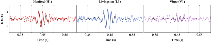
Figure 1: GW190521 observed by the H1 (left panel), L1 (middle panel) and V1 (right panel) detectors. Times are shown relative to May 21, 2019 at 03:02:29 UTC. Color curves: the detector time series are filtered with a 28–128 Hz band-pass filter and cleaned to remove 60 Hz power line. Black curves: signal reconstruction by cWB. The cWB reconstruction is in agreement with the amplitudes of GW190521 signal inside the detector noise.

Due to their high mass the IMBH binary systems are expected to merge at frequencies below 100 Hz while detector sensitivity is limited by seismic noise below 20 Hz. As a result, the detectors are mostly sensitive to the gravitational waves emitted at the final stages of the binary evolution, merger and ring-down. For IMBH binary systems the observed GW signal is short in duration and challenging to detect by template-based search pipelines. The excess power cWB Klimenko et al. (2016) is a template-independent search algorithm that uses minimal assumptions on the signal model to detect GWs. It does not depend on detailed waveform features such as the higher order modes, high mass ratios, misaligned spins, eccentric orbits and possible deviations from general relativity, and it operates even in cases where the lack of reliable models pose limitations for matched filtering methods. Therefore, cWB is suitable for detecting sources where reliable templates are not readily available Calderón Bustillo et al. (2018); Chandra et al. (2020).

First searches for gravitational waves from IMBH binaries were carried out with cWB on the data from the initial LIGO and Virgo observing runs (2005-2010) Abadie et al. (2012); Aasi et al. (2014a). A search for perturbed IMBH remnants was performed on the same data with the ring-down template search Aasi et al. (2014b). Later, the IMBH searches were conducted with O1 and O2 data both by cWB and the full inspiral-merger-ringdown template pipelines Abbott et al. (2017a, 2019b). The IMBH binary searches carried out on the O1 and O2 data produced the most stringent upper limit of $0.2\ \mathrm{Gpc}^{-3}\mathrm{yr}^{-1}$ on the IMBH merger rates Abbott et al. (2017a). Improvements of the Advanced detector sensitivities in the O3 run Abbott et al. (2016b) tripled the IMBH search volume resulting in the observation of the first IMBH binary event GW190521 Abbott et al. (2020c, d) identified by the cWB search with high confidence. Together with the first ever GW detection GW150914 Abbott et al. (2016a) and the heaviest BBH system GW170729 in the O1 and O2 data Abbott et al. (2019a), the GW190521 is yet another demonstration of cWB to detect unexpected binary sources.

In this paper, we demonstrate the capability of cWB to detect GW190521 with high confidence without the use of templates. We show that the cWB reconstruction of GW190521 is in agreement with the waveforms derived from LALInference Veitch et al. (2015) analysis. The main results of cWB analysis are presented in the discovery Abbott et al. (2020c) and astrophysical implication Abbott et al. (2020d) papers. In Section II we describe the details of GW190521 observation with cWB, including the low-latency analysis, the GW190521 sky localization and describe the detection significance established by cWB. In Section III we show consistency between the cWB waveform reconstruction and the best fits of the Bayesian inference waveforms from LALInference. We demonstrate and quantify that the cWB reconstruction is more consistent with waveforms from precessing BBHs rather than binaries with aligned spins. Appendices A, B and C outline the cWB searches in O3 and the detection procedure.

II Observation

II.1 Online detection and sky localization

The initial GW190521 trigger LIGO Scientific Collaboration, Virgo Collaboration (2019) was detected in low-latency by PyCBC Nitz et al. (2020) and cWB Klimenko et al. (2016) pipelines with the FARs 1 per 8.3 years and lower than 1 per 28 years respectively. The on-line cWB FAR was estimated using one day of coincident data around the trigger time. By combining all previously accumulated background data from the low-latency analysis, the GW190521 FAR was estimated to be lower than 1 per 500 years.

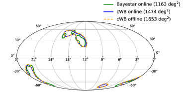
Figure 2: GW190521 90% credible areas source localization with the 3-detector LIGO-Virgo network reported by the low-latency analysis from Bayestar by using BBH templates Bohé et al. (2017) and cWB sky localization without templates for low-latency and offline analyses.

The waveform reconstructed by cWB in low-latency analysis (see Figure 1) did not show a typical chirping signal expected for BBH signals. Instead, GW190521 was a short signal with duration of 0.1 seconds and less than 4 cycles in the frequency band 30-80 Hz with almost symmetric shape. Such signal morphology is typical for the high mass BBH events when the system merges at low frequency where the sensitivity of the detectors is affected by seismic noise. Assuming that the binary merges at the peak signal frequency of 58 Hz (twice the orbital frequency), the total mass of the system in the detector frame should be exceeding 300 $M_{\odot}$ for equal mass BH components. The most plausible explanation for this signal is the merger of a binary BH system where the remnant is an intermediate mass black hole.

Figure 3: Time-frequency representation of GW190521 with a superposition of wavelet pixels selected by cWB. The pixel magnitudes are squared network signal-to-noise ratio. GW190521 does not show a chirping signal expected for binary systems.

In the low-latency analysis cWB estimated the sky area to be 1474 deg² (90% confidence interval). It is agreement with 1163 deg² (90% credible interval) reported initially with the public alert LIGO Scientific Collaboration, Virgo Collaboration (2019) and computed with the Bayestar Singer and Price (2016) sky localization algorithm using BBH templates Bohé et al. (2017). In the follow-up analysis, the sky maps were computed using calibrated data resulting in 1653 deg² and 765 deg² Abbott et al. (2020d) for cWB and Bayestar, respectively. Figure 2 compares the initially released skymaps with those computed by cWB for the HLV detector network.

II.2 Detection significance

The offline cWB analysis was conducted with the HL (LIGO Hanford and Livingston) and HLV (HL and Virgo) detector networks. Because of the difference in sensitivity between LIGO and Virgo detectors and larger non-stationary noise in Virgo Abbott et al. (2016b), the HL network was used to determine the detection significance of the GW190521 event, while the HLV network was used for waveform reconstruction described in Section III. As described in Abbott et al. (2020c), the data from GW detectors was conditioned prior to further analysis. Specifically for cWB analysis, we additionally mitigated the non-stationary noise coming from the anthropogenic activity (see Appendix B).

The detection significance of GW190521 was determined by time-shifting Hanford detector data with respect to the Livingston detector data to accumulate triggers of non-astrophysical origin. The time shifts were selected to be much longer (1 second or more) than the expected signal time delay between the detectors. To perform the background analysis we used 9.4 days of coincident data around the event inside the GPS time interval $[1241011102,1242485126]$. By using multiple time shifts, we accumulated an equivalent of $9,800$ years of the background data.

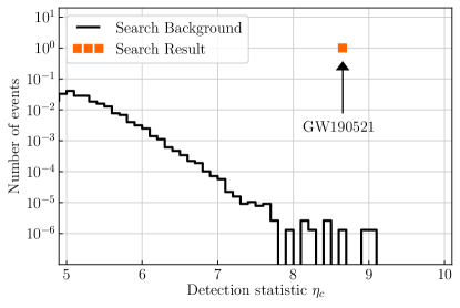
Figure 4: The search background that established the false-alarm rate of GW190521 to be 1 per 4900 years.

Figure 4 presents the background distribution of time-shifted data and the GW190521. Only two events have the cWB detection statistic $\eta_{c}$ higher than the GW190521 event, both consistent with random coincidences of short duration ($\approx$ 1 cycle) glitches observed in the LIGO frequency band 20–100 Hz. The amount of the background and the number of louder events results in a false-alarm rate of 1 per 4,900 years for GW190521, which constitutes a confident detection.

II.3 Search sensitivity

The detection range of IMBH sources has been increasing over time Abadie et al. (2012); Aasi et al. (2014a, b); Abbott et al. (2017a, 2019b), mainly due to improvements in the low-frequency regime of the GW detectors and the algorithms used. For the Advanced LIGO and Advanced Virgo, assuming the NRsur7dq4 signal model Varma et al. (2019), the detection ranges for events similar to GW190521 are 1.1 Gpc, 1.2 Gpc and 1.7 Gpc for O1, O2 and the first half of O3, respectively Abbott et al. (2020d). At present, the total search time-volume for events like GW190521 is $9.1\,\mathrm{Gpc}^{3}\,\mathrm{yr}$ Abbott et al. (2020d), which is the sum of the O1-O2 contribution, $3.2\,\mathrm{Gpc}^{3}\,\mathrm{yr}$ and of the nearly twice as large contribution from the first half of the O3 run: $5.9\,\mathrm{Gpc}^{3}\,\mathrm{yr}$.

The rate of the IMBH binary mergers was initially constrained from $1.3\times 10^{2}\,\mathrm{Gpc}^{-3}\,\mathrm{yr}^{-1}$ using the 2005-2007 data set Abadie et al. (2012), and later to $0.2\,\mathrm{Gpc}^{-3}\,\mathrm{yr}^{-1}$ with data from the first two LIGO-Virgo observing runs Abbott et al. (2017a). Now we estimate that the rate of events similar to GW190521 is $0.13_{-0.11}^{+0.3}\,\mathrm{Gpc}^{-3}\,\mathrm{yr}^{-1}$ Abbott et al. (2020d) that is below the previously derived upper limits.

III Waveform analysis

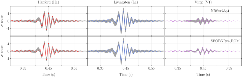
Figure 5: Visualization of the consistency of the signal-agnostic measurement by cWB with two alternative models in time domain: upper panel NRSur7dq4 model, lower panel SEOBNRv4_ROM model. The colored curves are the whitened waveform for GW190521 as reconstructed by cWB for the LIGO Hanford (red), LIGO Livingston (blue) and Virgo (violet); they are a direct measurement and do not change from the upper to the lower panels. The shaded belts are 90% confidence intervals per each time sample at each detector and are model dependent.

In this section, we present the comparison of the GW190521 reconstruction by cWB with the LALInference model-based Bayesian reconstruction Veitch et al. (2015); Ashton et al. (2019). The purpose of this comparison is to demonstrate if the cWB and LALInference reconstructions are consistent for different signal models.

The cWB waveforms are derived directly from the data in the wavelet (time-frequency) domain Necula et al. (2012) by selecting the excess power data samples above the average fluctuations of the detector noise. The cWB point estimate of the signal waveform in each detector is constructed as a linear combination of selected wavelets with the amplitudes defined by the constrained maximum likelihood method Klimenko et al. (2016). Similar to the band-pass filter shown in Figure 1 cWB performs the time-frequency filtering of data. Such signal-agnostic reconstruction may capture significant features of the signal that may not be well described by the model approximations and help to identify limitations of the models used for Bayesian inference of GW190521. On the other hand, due to the excess power threshold, the low SNR wavelet components could be excluded from the cWB analysis resulting in a partial reconstruction of the GW190521 signal. In addition, the non-Gaussian noise fluctuations may bias the cWB reconstruction and add systematic errors not accounted for by the Bayesian inference. Therefore, a direct comparison of the cWB reconstruction, or any other excess power algorithm, with the best matching LALInference waveforms is not straightforward and requires a more accurate statistical treatment as described below.

In this analysis we compare cWB point estimate waveform with the effective-one-body model SEOBNRv4_ROM Ossokine et al. (2020); Babak et al. (2017) and the numerical relativity surrogate model NRSur7dq4 Varma et al. (2019), which is the preferred model for the GW190521 event. For correct comparison with the cWB point estimate, the simulated signals from the both models are treated exactly in the same way as the real GW signal: simulated signals are selected randomly from the LALInference posterior distribution, injected into the data (in the time interval of 4096 seconds around the GW190521 event) and analysed with cWB. Then we use the cWB reconstruction to produce the off-source point estimate for each of the simulated events. These off-source simulations take into account the fluctuations of the real detector noise, cWB reconstruction errors and the variability of the signal model in the LALInference posterior distribution. The off-source simulations are synchronized in time and used for the construction of confidence intervals showing the expected spread of the modeled signal amplitudes as seen by cWB, which can be directly compared with the cWB point estimate for GW190521.

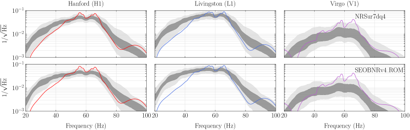
Figure 6: Visualization of the consistency of the signal-agnostic measurement by cWB with two alternative models in frequency domain: upper panel NRSur7dq4 model, lower panel SEOBNRv4_ROM model. The colored curves are the whitened waveform spectra for GW190521 as reconstructed by cWB for the LIGO Hanford (red), LIGO Livingston (blue) and Virgo (violet); they are a direct measurement form the data and do not change from the upper to the lower panels. The dark shaded belts are the 50% confidence intervals per each frequency bin showing the variation of the model spectral amplitudes. The light shaded belts are the 90% confidence intervals.

The result is shown in Figure 5 where the 90% confidence intervals are calculated from whitened waveforms of approximately 1400 simulated events. They display that with 90% probability the local amplitudes of the GW190521 signal filtered by cWB are located within these boundaries. The cWB reconstruction of GW190521 comprises about 11 degrees of freedom (the effective number of independent wavelets), so confidence intervals for the contiguous time values are correlated. An approximate estimate of how frequently one should expect at least one deviation outside the belt ensuring 90% confidence is given by $1-e^{-11\times 0.1}$ or approximately 70%. The local deviations outside of the 90% interval visible in top plots for the NRSur7dq4 models are negligible. However, the SEOBNRv4_ROM model appears to have larger deviation at the beginning of the GW190521 signal. The difference between the two models is also observed in the frequency domain. Figure 6 shows 90% confidence intervals built from the Fourier representation of the whitened off-source reconstructions of simulated events. This analysis highlights more discrepancy between NRSur7dq4 and SEOBNRv4_ROM models than in the time domain. In particular, at lower frequency the NRSur7dq4 model shows a deficit of energy in comparison with the spin-aligned SEOBNRv4_ROM model, demonstrating a better agreement with the cWB reconstruction of GW190521. Such a deficit of energy before the merger is expected for signals with orbital precession predicted by the NRSur7dq4 model or signals with large eccentricity Calderón Bustillo et al. (2020).

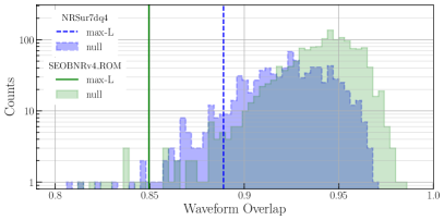
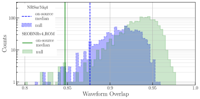
Figure 7: The quantitative comparison of whether the signal models are consistent with cWB reconstruction of GW190521. The plots show the off-source (null) distributions and calculated waveform overlaps for GW190521. Left panel: the max-L is assumed to be a representative waveform for GW190521. Right panel: any posterior waveform is assumed to be a valid representation of GW190521. In both cases, the p-values are 7.9% and 1.0% for NRSur7dq4 and SEOBNRv4_ROM, respectively. It indicates that SEOBNRv4_ROM is less consistent with GW190521 but its relatively large p-value does not allow to confidently exclude this model.

III.1 Waveform overlap

The time and frequency confidence intervals is a convenient tool to identify local waveform differences between the cWB reconstruction of GW190521 and the signal model. However, they do not provide a statistical measure for disagreement between a given model and the GW190521 signal. To quantify the consistency between different waveforms, we use the waveform overlap, or the match Abbott et al. (2020c); Salemi et al. (2019), between the cWB point estimate $\mathbf{w}=\{w_{k}(t)\}$ and a selected whitened waveform from a given signal model $\mathbf{h}=\{{h}_{k}(t)\}$:

$$\mathrm{O}(\mathbf{w},\mathbf{h})=\frac{(\mathbf{w}|\mathbf{h})}{\sqrt{(\mathbf{w}|\mathbf{w})}\sqrt{(\mathbf{h}|\mathbf{h})}}\,.$$ (1)

The scalar product $(.|.)$ is defined in the time domain as

$$(\mathbf{w}|{\mathbf{h}})=\sum_{k}\int_{t_{1}}^{t_{2}}{w}_{k}(t){h}_{k}(t)dt,$$

where the index $k$ running over the detectors and $[t_{1},t_{2}]$ is the time range of the reconstructed event. First, we calculate the distribution of $\mathrm{O}_{0}(\mathbf{w_{i}},\mathbf{h_{i}})$ for the off-source injections, where the waveform $\mathbf{h_{i}}$ is drawn randomly from the posterior distribution and the $\mathbf{w_{i}}$ is the cWB point estimate of $\mathbf{h_{i}}$. The $\mathrm{O}_{0}$ gives us the null distribution expected for a given signal model accounting for systematic uncertainties due to non-Gaussian detector noise and the cWB reconstruction. Second, we calculate the overlap $\mathrm{O}(\mathbf{W},\mathbf{h_{p}})$ where $\mathbf{W}$ is the on-source cWB reconstruction of GW190521 and $\mathbf{h_{p}}$ is a proxy of the true GW190521 signal selected from the posterior distribution. If the model accurately describes the GW190521 event, we expect that the overlap $\mathrm{O}(\mathbf{W},\mathbf{h_{p}})$ falls within the null distribution, which can be characterized with the p-value - the fraction of entries in the null distribution with the overlap below $\mathrm{O}(\mathbf{W},\mathbf{h_{p}})$. Left panel in Figure 7 shows the null distribution and the overlap with the maximum likelihood (max-L) template, used as the proxy $\mathbf{h_{p}}$ for the GW190521 signal, evaluated for both signal models. The max-L overlaps are 0.89 and 0.85, while the p-values are 7.9% and 1.0% for the NRSur7dq4 and SEOBNRv4_ROM models, respectively. In agreement with Figures 5 and 6, this figure illustrates that the latter signal model is less consistent with the GW190521 event. However, the relatively large p-value of 1% does not allow us confident exclusion of the SEOBNRv4_ROM as a model for GW190521.

The assumption of the max-L waveform being the best representation of GW190521 is viable but not exclusive. The maximum posterior waveform could also be used instead of the max-L. In addition to this ambiguity, a selection of any specific proxy waveform $\mathbf{h_{p}}$ introduces a bias in the calculation of the p-value. To eliminate this bias, for each off-source injection $\mathbf{h_{i}}$ we should run the LALinference parameter estimation to find the corresponding proxy waveform, which should be used instead of $\mathbf{h_{i}}$ for the calculation of the null distribution. This is not practically feasible due to the high computational cost of the LALinference analysis. Instead, we modify the statistical procedure in order to reduce the selection bias. In general, for a correct model, any posterior waveform could be a fair proxy $\mathbf{h_{p}}$ for the GW190521 signal. Therefore, we calculate the on-source overlap distribution $\mathrm{O}(\mathbf{W},\mathbf{h_{i}})$ by randomly drawing $\mathbf{h_{i}}$ from the posterior distribution. Instead of selecting a specific $\mathrm{O}(\mathbf{W},\mathbf{h_{p}})$ overlap, we calculate the median of the on-source distribution. Similarly, a set of distributions $\mathrm{O}(\mathbf{w_{j}},\mathbf{h_{i}})$ can be calculated for any cWB point estimate $\mathbf{w_{j}}$ from the off-source injections. By calculating the median of each $\mathrm{O}(\mathbf{w_{j}},\mathbf{h_{i}})$ distribution we can build a new null distribution for the median of $\mathrm{O}(\mathbf{W},\mathbf{h_{i}})$. The right panel of Figure 7 shows these null distributions and the on-source median overlap values of 0.88 and 0.85 for the NRSur7dq4 and SEOBNRv4_ROM models, respectively. The corresponding p-values are 7.9% and 1.0%. These numbers are similar to the results obtained with the analysis using the max-L waveform. Nevertheless, the comparison of the entire posterior distribution with the corresponding off-source null distributions provide a more robust test of the GW190521 models.

IV Summary

The cWB searches for GW transients have demonstrated confident detection of binary black holes, including the first gravitational-wave signal GW150914 detected in the O1 run Abbott et al. (2016a), the heaviest BBH system GW170729 detected in the O2 run together with the other detection from the first two observing runs of Advanced LIGO and Advanced Virgo Abbott et al. (2019a). The observation of GW190521, the first confident detection of an IMBH by cWB, is yet another demonstration of its capabilities to discover new GW sources. The cWB detection in low-latency provided a robust reconstruction of GW190521 including a sky map that was in agreement with the template based searches. The offline cWB analysis provided a confident detection of GW190521 with the false-alarm rate of 1 per 4,900 years. The estimated rate of events similar to GW190521 ($0.13_{-0.11}^{+0.3}\,\mathrm{Gpc}^{-3}\,\mathrm{yr}^{-1}$ Abbott et al. (2020d)) is below the previously derived upper limits. The waveform analysis presented in the paper demonstrates the agreement between cWB and LALInference reconstructions for different signal models. The consistency between signal models and cWB reconstruction is described by p-values, which are 7.9% and 1.0% for the NRSur7dq4 and SEOBNRv4_ROM models respectively. While the p-value of NRSur7dq4 shows that this model is consistent with the cWB reconstruction of GW190521, the relatively large p-value for SEOBNRv4_ROM signal model does not allow us to confidently exclude this model.

The anticipated sensitivity improvements of the GW instruments at low-frequency Abbott et al. (2016b) can lead to detections of more IMBH sources. These sources could be formed dynamically and may have waveforms not covered by existing templates. The template-independent search has a potential to play an important role in the detection of such signals and help us to explore the physical properties of IMBH sources in a wide range of masses.

V Acknowledgments

This research has made use of data, software and/or web tools obtained from the Gravitational Wave Open Science Center, a service of LIGO Laboratory, the LIGO Scientific Collaboration and the Virgo Collaboration. The work by S. K. was supported by NSF Grant No. PHY 1806165. We gratefully acknowledge the support of LIGO and Virgo for provision of computational resources. IB acknowledges support by the National Science Foundation under grant No. PHY 1911796, the Alfred P. Sloan Foundation and by the University of Florida.

Appendix A Coherent WaveBurst

Coherent WaveBurst (cWB) is a search algorithm for detection and reconstruction of GW transient signals operating without a specific waveform model. cWB searches for a coincident signal power in multiple detectors for signals with the duration up to a few seconds. The analysis is performed in the wavelet domain Necula et al. (2012) on data normalized (whitened) by the amplitude spectral density of the detector noise. The cWB selects wavelets with amplitudes above the fluctuations of the detector noise and groups them into clusters. For clusters correlated in multiple detectors, cWB identifies coherent events and reconstructs the source sky location and signal waveforms with the constrained maximum likelihood method Klimenko et al. (2016).

The cWB detection statistic is based on the coherent network energy $E_{\rm c}$ obtained by cross-correlating data in different detectors; $\sqrt{E_{\rm c}}$ is the estimator of the coherent network SNR Klimenko et al. (2016). The agreement between GW data and cWB reconstruction is characterized by a chi-squared statistic $\chi^{2}=E_{\rm n}/N_{\rm df}$, where $E_{\rm n}$ is the residual energy estimated after the reconstructed waveforms are subtracted from the whitened data, and $N_{\rm df}$ is the number of independent wavelet amplitudes describing the event. GW190521 is identified in LIGO data with $\chi^{2}=0.68$, showing no evidence for residual energy inconsistent with Gaussian noise. The cWB detection statistic is $\eta_{\rm c}=\sqrt{E_{\rm c}/\max(\chi^{2},1)}$, where the $\chi^{2}$ correction improves the robustness of the pipeline against non-Gaussian detector noise. Events with $\eta_{\rm c}>5$ are stored by the pipeline for further processing.

To improve the robustness of the algorithm against non-stationary detector noise (glitches) and reduce the rate of false alarms, cWB uses signal-independent vetoes. The primary veto cuts are on the network correlation coefficient $c_{\rm c}=E_{\rm c}/(E_{\rm c}+E_{\rm n})$ and the $\chi^{2}$. For a GW signal the expected values of both statistics are close to unity and the candidate events with $c_{\rm c}<0.7$ and $\chi^{2}>2.5$ are rejected as potential glitches.

Appendix B Mitigation of non-stationary detector noise

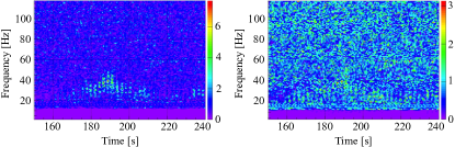
Figure 8: Time-frequency WDM wavelet decomposition of a segment of LLO data: left (right) - before (after) application of the LPE filter. The excess power due to anthropogenic ground motion is reduced.

The analysis of the early O3 data revealed several dominant sources of non-stationary noise (glitches). The dominant sources of this noise are the low frequency glitches below 50 Hz due to anthropogenic ground motion and the short duration (blip) glitches in the frequency band $50-300$ Hz Abbott et al. (2017b); Cabero et al. (2019). The anthropogenic ground motion in LIGO Livingston (LLO) produced the scattered light noise below 50 Hz Abbott et al. (2020c) appearing as a periodic sequence of short duration transients. A similar type of noise is also observed in the LIGO Hanford (LHO) detector, but at a significantly lower rate. Left panel of Figure 8 shows the example of scatter light glitches in the time-frequency map of the LLO data segment. This noise is highly periodic with the two characteristic times of 2.35 s and 0.235 s. It can be corrected with the linear predictor error filter (LPE) Tiwari et al. (2015) as shown in the right panel of Figure 8. The correction of the wavelet data was performed in the frequency band $16-48$ Hz and does not affect the detection and reconstruction of signals at higher frequency. No scattered light glitches were observed at the time of GW190521, which has the peak frequency of 58 Hz. The application of the LPE filter significantly reduces the rate of the scattered light glitches and improves the detection of IMBH binary signals expected at low frequencies.

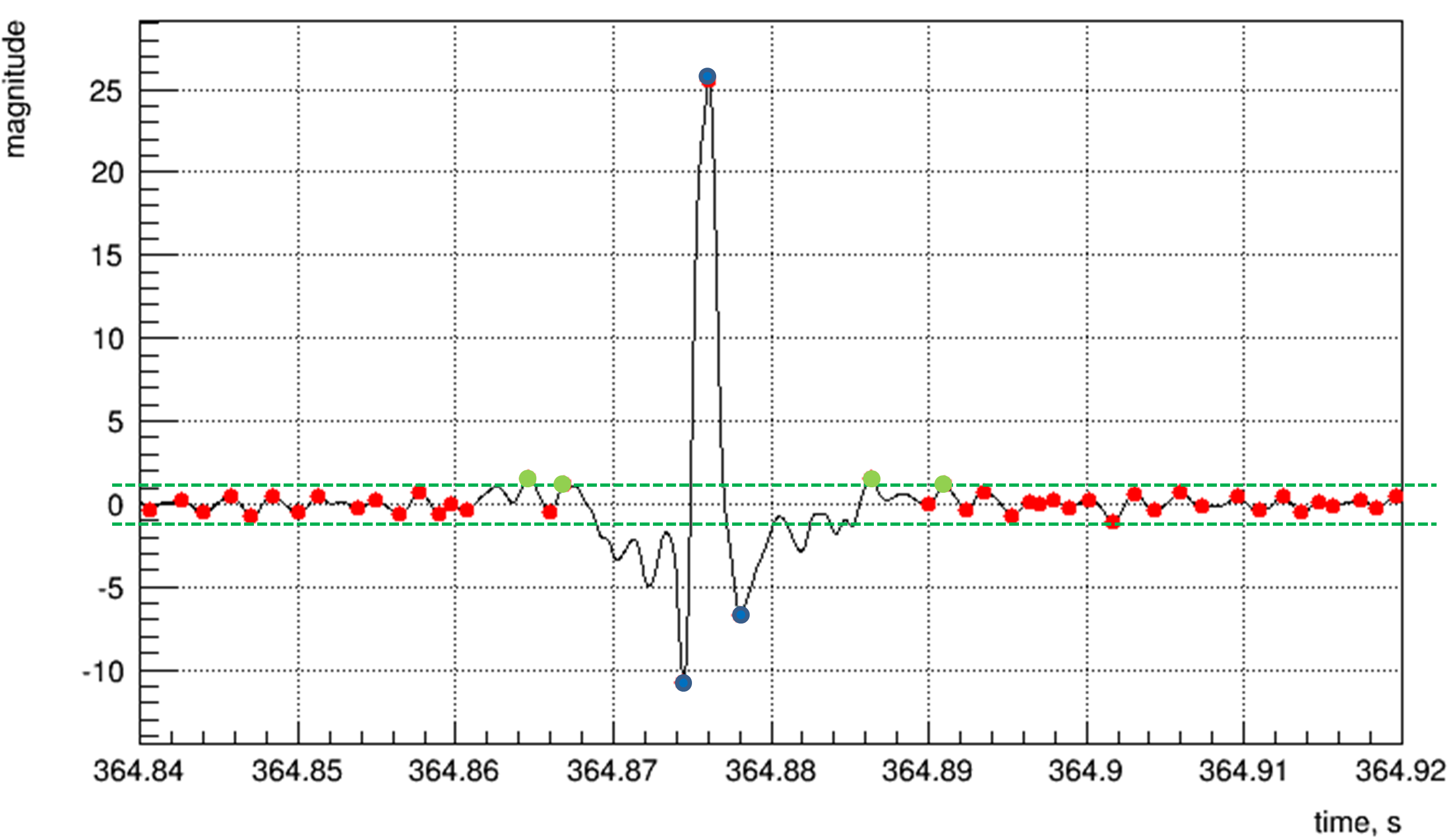
Figure 9: An example of a blip glitch. The characteristic waveforms of blip glitches allow us to distinguish them from gravitational waves and other sources of noise as described in the text.

Case	1	2	3	4	5	6	7	8
IMBH configuration	IMBH,BBH	-	IMBH	-	IMBH	BBH	BBH	-
BBH configuration	-	IMBH,BBH	-	BBH	BBH	IMBH	-	IMBH
False-alarm rate	IMBH	BBH	IMBH	BBH	min(BBH,IMBH)$\times 2$

Table 1: Possible detection cases and corresponding trial factors. For example, in case 5, an event is identified in both search configurations but the peak frequencies are reconstructed in different bands, so the smaller false-alarm rate from the two configurations multiplied by a trial factor of 2 defines the event’s significance. The calculation of GW190521 significance is given by case 3.

The short noise transients are primarily blip glitches present in all observing runs and their origin is yet unknown Abbott et al. (2017b); Cabero et al. (2019). The properties of blip glitches have been extensively studied in the previous observing runs Abbott et al. (2016) and to remove them we apply a similar method used in the previous cWB searches Abbott et al. (2019a, b). The waveforms are typically time-symmetric, with less than one cycle, and without a clear frequency evolution. The duration is usually of an order of $O(10)$ ms and bandwidth $O(100)$ Hz. Figure 9 shows an example of a blip glitch. The characteristic waveform of blip glitches allows us for their simple classification as follows. The energy of the data samples with the largest magnitude ($A_{m}$) and two peak amplitudes around it (blue dots) is denoted as $E_{0}$. The remaining samples with the amplitudes outside of the thresholds $\pm A_{m}$/7.6 (green dots) have the energy denoted as $E_{1}$. The ratio $Q=E_{1}/E_{0}$ is calculated for each detector used to reconstruct an event and a smallest value of $Q$ out of all detectors may indicate the presence of a blip glitch. Events with $Q<0.1$ are removed from the further analysis. GW190521 with a $Q$ value of 0.55 passed this criteria.

Appendix C Search configurations

A generic search for binary systems covers a large parameter space. It is not possible to design a search optimized to all binaries because the frequency content of their GW signals can vary significantly. In general, GW signals have the peak frequency $f_{peak}\propto 1/M_{tot}$, where $M_{tot}$ is the binary total mass in the detector frame. Lighter binaries with $M_{tot}\approx 2$ $M_{\odot}$ merge at high frequency and their GW signal may be observable in the detector data for hundreds of seconds. Heavier systems with $M_{tot}>100$ $M_{\odot}$ merge at lower frequencies and their detected signals are less than a second long. Therefore, a generic search for binary systems is split into the two search configurations. One configuration focuses on the IMBH binaries ($f_{peak}<80$ Hz), while the other configuration is used for detection of stellar mass BBHs ($f_{peak}>80$ Hz). Because the detector noise and glitches vary significantly in these two frequency bands, the searches require different selection cuts.

The two configurations are not disjoint and trial factors need to be considered to calculate events significance and they are determined by the reconstructed peak frequencies. Table 1 summarizes all cases when a binary system is detected either by the BBH or IMBH search configuration. For example, if the event is detected in both search configurations with the peak frequencies above 80 Hz, then the BBH search is selected and the significance of the event is not penalized by the trial factor. In contrast, if the peak frequencies of detected signals are reconstructed in different frequency bands, then the smaller FAR is used for calculation of the event’s significance and it is multiplied by a trial factor of 2.

References

- Aasi et al. (2015) J. Aasi et al. (LIGO Scientific), Class. Quant. Grav. 32, 074001 (2015), arXiv:1411.4547 [gr-qc] .
- Acernese et al. (2015) F. Acernese et al. (VIRGO), Class. Quant. Grav. 32, 024001 (2015), arXiv:1408.3978 [gr-qc] .
- Abbott et al. (2020a) B. P. Abbott et al. (LIGO Scientific Collaboration and Virgo Collaboration), Phys. Rev. Lett. 892, L3 (2020a), arXiv:2001.01761 [astro-ph.HE] .
- Abbott et al. (2020b) B. P. Abbott et al. (LIGO Scientific Collaboration and Virgo Collaboration), arXiv e-prints , arXiv:2004.08342 (2020b), arXiv:2004.08342 [astro-ph.HE] .
- Abbott et al. (2020c) B. P. Abbott et al. (LIGO Scientific Collaboration and Virgo Collaboration), Phys. Rev. Lett. 125, 101102 (2020c).
- Gra (2020) “Gravitational-Wave Candidate Event Database, LIGO/Virgo Public Alerts,” (2020).
- Ebisuzaki et al. (2001) T. Ebisuzaki, J. Makino, T. G. Tsuru, Y. Funato, S. F. Portegies Zwart, P. Hut, S. McMillan, S. Matsushita, H. Matsumoto, and R. Kawabe, Astrophys. J. 562, L19 (2001), arXiv:astro-ph/0106252 [astro-ph] .
- Mezcua (2017) M. Mezcua, International Journal of Modern Physics D 26, 1730021 (2017), arXiv:1705.09667 .
- Abbott et al. (2016a) B. P. Abbott et al. (LIGO Scientific Collaboration, Virgo Collaboration), prl 116, 061102 (2016a), arXiv:1602.03837 [gr-qc] .
- Abbott et al. (2019a) B. P. Abbott et al. (LIGO Scientific, Virgo), Phys. Rev. X9, 031040 (2019a), arXiv:1811.12907 [astro-ph.HE] .
- Spera and Mapelli (2017) M. Spera and M. Mapelli, Mon. Not. Roy. Astron. Soc. 470, 4739 (2017), arXiv:1706.06109 [astro-ph.SR] .
- Woosley (2017) S. E. Woosley, Astrophys. J. 836, 244 (2017), arXiv:1608.08939 [astro-ph.HE] .
- Giacobbo et al. (2018) N. Giacobbo, M. Mapelli, and M. Spera, Mon. Not. Roy. Astron. Soc. 474, 2959 (2018), arXiv:1711.03556 [astro-ph.SR] .
- Belczynski et al. (2016) K. Belczynski et al., Astron. Astrophys. 594, A97 (2016), arXiv:1607.03116 [astro-ph.HE] .
- Klimenko et al. (2016) S. Klimenko et al., prd 93, 042004 (2016), arXiv:1511.05999 [gr-qc] .
- Calderón Bustillo et al. (2018) J. Calderón Bustillo, F. Salemi, T. Dal Canton, and K. P. Jani, Phys. Rev. D 97, 024016 (2018), arXiv:1711.02009 [gr-qc] .
- Chandra et al. (2020) K. Chandra, V. Gayathri, J. C. Bustillo, and A. Pai, Phys. Rev. D 102, 044035 (2020).
- Abadie et al. (2012) J. Abadie et al. (LIGO Scientific, VIRGO), Phys. Rev. D85, 102004 (2012), arXiv:1201.5999 [gr-qc] .
- Aasi et al. (2014a) J. Aasi et al., prd 89, 122003 (2014a), arXiv:1404.2199 [gr-qc] .
- Aasi et al. (2014b) J. Aasi et al., prd 89, 102006 (2014b), arXiv:1403.5306 [gr-qc] .
- Abbott et al. (2017a) B. P. Abbott et al. (LIGO Scientific, Virgo), Phys. Rev. D96, 022001 (2017a), arXiv:1704.04628 [gr-qc] .
- Abbott et al. (2019b) B. P. Abbott et al. (LIGO Scientific, Virgo), Phys. Rev. D100, 064064 (2019b), arXiv:1906.08000 [gr-qc] .
- Abbott et al. (2016b) B. P. Abbott et al. (KAGRA Collaboration, LIGO Scientific Collaboration, Virgo Collaboration), Living Rev. Rel. 19, 1 (2016b), arXiv:1304.0670 [gr-qc] .
- Abbott et al. (2020d) B. P. Abbott et al., The Astrophysical Journal 900, L13 (2020d).
- Veitch et al. (2015) J. Veitch, V. Raymond, B. Farr, et al., prd 91, 042003 (2015), arXiv:1409.7215 [gr-qc] .
- LIGO Scientific Collaboration, Virgo Collaboration (2019) LIGO Scientific Collaboration, Virgo Collaboration, gcn 24621 (2019).
- Nitz et al. (2020) A. Nitz, I. Harry, D. Brown, C. M. Biwer, J. Willis, T. Dal Canton, C. Capano, L. Pekowsky, T. Dent, A. R. Williamson, S. De, G. Davies, M. Cabero, D. Macleod, B. Machenschalk, S. Reyes, P. Kumar, T. Massinger, F. Pannarale, dfinstad, M. Tápai, S. Fairhurst, S. Khan, L. Singer, A. Nielsen, S. Kumar, shasvath, idorrington92, H. Gabbard, and B. U. V. Gadre, “gwastro/pycbc v1.15.3,” (2020).
- Bohé et al. (2017) A. Bohé et al., prd 95, 044028 (2017), arXiv:1611.03703 [gr-qc] .
- Singer and Price (2016) L. P. Singer and L. Price, prd 93, 024013 (2016), arXiv:1508.03634 [gr-qc] .
- Varma et al. (2019) V. Varma, S. E. Field, M. A. Scheel, J. Blackman, D. Gerosa, L. C. Stein, L. E. Kidder, and H. P. Pfeiffer, Phys. Rev. Research. 1, 033015 (2019), arXiv:1905.09300 [gr-qc] .
- Ashton et al. (2019) G. Ashton et al., Astrophys. J. Suppl. 241, 27 (2019), arXiv:1811.02042 [astro-ph.IM] .
- Necula et al. (2012) V. Necula, S. Klimenko, and G. Mitselmakher, Gravitational waves. Numerical relativity - data analysis. Proceedings, 9th Edoardo Amaldi Conference, Amaldi 9, and meeting, NRDA 2011, Cardiff, UK, July 10-15, 2011, J. Phys. Conf. Ser. 363, 012032 (2012).
- Ossokine et al. (2020) S. Ossokine et al., Phys. Rev. D 102, 044055 (2020), arXiv:2004.09442 [gr-qc] .
- Babak et al. (2017) S. Babak, A. Taracchini, and A. Buonanno, Phys. Rev. D95, 024010 (2017), arXiv:1607.05661 [gr-qc] .
- Calderón Bustillo et al. (2020) J. Calderón Bustillo, N. Sanchis-Gual, A. Torres-Forné, and J. A. Font, arXiv e-prints , arXiv:2009.01066 (2020), arXiv:2009.01066 [gr-qc] .
- Salemi et al. (2019) F. Salemi, E. Milotti, G. A. Prodi, G. Vedovato, C. Lazzaro, S. Tiwari, S. Vinciguerra, M. Drago, and S. Klimenko, Phys. Rev. D 100, 042003 (2019).
- Abbott et al. (2017b) B. P. Abbott et al. (LIGO Scientific Collaboration, Virgo Collaboration), Submitted to Class. Quant. Grav. (2017b), arXiv:1710.02185 [gr-qc] .
- Cabero et al. (2019) M. Cabero et al., Class. Quant. Grav. 36, 155010 (2019), arXiv:1901.05093 [physics.ins-det] .
- Tiwari et al. (2015) V. Tiwari, M. Drago, V. Frolov, S. Klimenko, G. Mitselmakher, V. Necula, G. Prodi, V. Re, F. Salemi, G. Vedovato, and I. Yakushin, Classical and Quantum Gravity 32, 165014 (2015), arXiv:1503.07476 [gr-qc] .
- Abbott et al. (2016) B. P. Abbott, R. Abbott, T. D. Abbott, et al. (LIGO Scientific Collaboration, Virgo Collaboration), Class. Quant. Grav. 33, 134001 (2016), arXiv:1602.03844 [gr-qc] .