Convergence of Gibbs Sampling:
Coordinate Hit-and-Run Mixes Fast

Abstract

Gibbs sampling, also known as Coordinate Hit-and-Run (CHAR), is a Markov chain Monte Carlo algorithm for sampling from high-dimensional distributions. In each step, the algorithm selects a random coordinate and re-samples that coordinate from the distribution induced by fixing all the other coordinates. While this algorithm has become widely used over the past half-century, guarantees of efficient convergence have been elusive. We show that the Coordinate Hit-and-Run algorithm for sampling from a convex body $K$ in $\mathbb{R}^{n}$ mixes in $O^{*}(n^{9}R^{2}/r^{2})$ steps, where $K$ contains a ball of radius $r$ and $R$ is the average distance of a point of $K$ from its centroid. We also give an upper bound on the conductance of Coordinate Hit-and-Run, showing that it is strictly worse than Hit-and-Run or the Ball Walk in the worst case.

1 Introduction

Sampling from a distribution in high-dimensional space is a fundamental problem and an essential ingredient of algorithms for optimization, integration, statistical inference, and other applications. Progress on sampling algorithms has led to many useful tools, both theoretical and practical. In the most general setting, given access to a function $f:\mathbb{R}^{n}\rightarrow\mathbb{R}_{+},$ the goal is to generate a point $x$ whose density is proportional to $f(x)$. Two special cases of particular interest are when $f$ is uniform over a convex body and when $f$ is a Gaussian restricted to a convex set.

The general approach to sampling is to design an ergodic, time-reversible Markov chain whose state space is the convex body and which has the desired density as its stationary distribution. The key question is to bound the rate of convergence of the Markov chain. The Ball walk [17, 14, 22] and Hit-and-Run [2, 25, 20] are two Markov chains that work in full generality and have been shown to mix rapidly (i.e., the convergence rate is polynomial in ambient dimension) for arbitrary log-concave densities. Three decades of improvements have reduced the complexity of this problem to a small polynomial in the dimension. For a log-concave density with support of diameter $D$, the mixing time of both Ball Walk and Hit-and-Run is $O^{*}(n^{2}D^{2})$, each step requiring $O(n^{2})$ function evaluations and $O(n^{2})$ arithmetic operations, giving total arithmetic complexity of $O^{*}(n^{4}D^{2})$[14, 18, 20].

A simple and widely-used algorithm that pre-dates these developments is the Gibbs Sampler, proposed by Turchin in 1971 [27]. It is inspired by statistical physics and is commonly used for sampling distributions [6, 7] and Bayesian inference [9, 10, 11]. To sample from a multivariate density, at each step, the Gibbs sampling algorithm selects a coordinate (either at random or in order, cycling through the coordinates), fixes all other coordinates, and re-samples this coordinate from the induced distribution. This algorithm is very similar to Hit-and-Run, except that instead of picking a direction uniformly at random from the unit sphere, it is picked only from one of the $n$ basis vectors (see [1] for a historical account and more background). It was reported to be significantly faster than Hit-and-Run in state-of-the-art software for volume computation and integration [3, 8, 5]. Gibbs sampling, also called Coordinate Hit-and-Run, has a computational benefit: updating the current point takes $O(n)$ time rather than $O(n^{2})$ even for polyhedra since the update is along only one coordinate direction. Thus the overhead per step is reduced from $O(n^{2})$, as in all previous algorithms, to $O(n)$. However, despite half a century of intense study, the convergence rate of Gibbs sampling has remained an open problem.

This paper shows that Gibbs sampling/Coordinate Hit-and-Run mixes rapidly for any convex body $K$. Before stating our main theorem formally, we define the Coordinate Hit-and-Run.

Coordinate Hit-and-Run.

Algorithm 1 describes the Coordinate Hit-and-Run Markov chain, hereafter referred to as CHAR, for sampling uniformly from a convex body $K\in\mathbb{R}^{n}$. Let $\{e_{i}:i\in[n]\}$ be the standard basis for $\mathbb{R}^{n}.$ The input to the algorithm is the convex body $K$, a starting point $x^{(0)}$ in the interior of $K$, and the number of steps $T$.

Input: a point $x^{(0)}\in K$, integer $T$.

for $i=1,2,\cdots,T$ do

      

      Pick a uniformly random axis direction $e_{j}$

      Set $x^{{(i)}}$ to be a random point along the line $\ell=\left\{x^{(i-1)}+te_{j}\,:\>t\in\mathbb{R}\right\}$ chosen uniformly from $\ell\cap K$.

end for

Output: $x^{{(T)}}$.

Algorithm 1 Coordinate Hit-and-Run (CHAR)

The stationary distribution of the Coordinate hit-and-run walk is the uniform distribution $\pi_{K}$ over $K$. To sample from a general log-concave density $f:\mathbb{R}^{n}\rightarrow\mathbb{R}_{+}$ the only change is in Step 2, where the next point $y$ is chosen according to $f(y)$ restricted to $\ell$. In both cases, the process is symmetric and ergodic, so the stationary distribution of the Markov chain is the desired distribution.

We can now state our main theorem (see Sec. 1.1 for the definition of a warm start).

Theorem 1.

Let $K$ be a convex body in $\mathbb{R}^{n}$ containing a unit ball. Let $R^{2}$ be the expected squared distance of a uniformly random point in $K$ from the centroid of $K$, and let $\pi_{K}$ denote the uniform distribution on $K$. Let $\sigma$ be a starting distribution and let $\sigma^{m}$ be the distribution of the current point after $m$ steps of Coordinate Hit-and-Run in $K$. Let $\varepsilon>0$, and suppose that $\sigma$ is $M$-warm with respect to $\pi_{K}$. Then for

$$m>7\cdot 10^{4}\cdot\frac{M^{2}R^{2}n^{9}}{\varepsilon^{2}}\log\left(\frac{2M}{\varepsilon}\right),$$

the total variation distance between $\sigma^{m}$ and $\pi_{K}$ is less than $\varepsilon$.

By applying an affine transformation, $R$ can be made $O(\sqrt{n})$ (see [4], [14], [21]). We note that from a warm start, both the Ball Walk and Hit-and-Run have a mixing time of $O^{*}(n^{2}R^{2})$ [14, 20]. While our bound is likely not the best polynomial bound for CHAR, in Section 4, we show that it is necessarily higher than the bound for Hit-and-Run.

Concurrently and independently, Narayanan and Srivastava [23] also proved a polynomial bound on the mixing rate of Coordinate Hit-and-Run, with a different proof. They showed that CHAR mixes in $O^{*}(n^{7}R_{1}^{4})$ steps where $R_{1}$ is the smallest number s.t., $B_{\infty}\subseteq K\subseteq R_{1}B_{\infty}$, i.e., the cube sandwiching ratio ($R_{1}$ can be larger than $R$ in our theorem by a factor of $\sqrt{n}$). After an affine transformation, $R_{1}$ can be bounded by $O(n)$.

A key ingredient of our proof is a new “$\ell_{0}$”-isoperimetric inequality. We will need the following definition.

Definition 1 (Axis-disjoint).

Two measurable sets $S_{1},S_{2}$ are called axis-disjoint if $\forall x\in S_{1},\forall y\in S_{2},|\{i\in\left[n\right]:x_{i}=y_{i}\}|\leq n-2$.

In other words, it is not possible to move from a point in $S_{1}$ to any point in $S_{2}$ in one step of CHAR and vice versa (see Fig. 1).

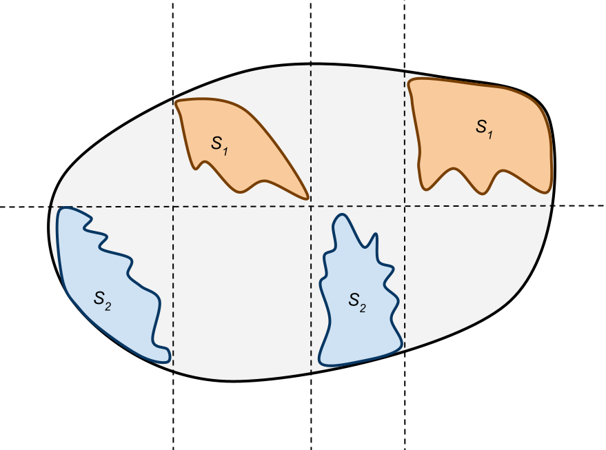
Figure 1: Axis-disjoint subsets $S_{1}$ and $S_{2}$.

The main component of the proof of Theorem 1 is the following isoperimetric inequality for axis-disjoint subsets of a convex body.

Theorem 2.

Let $K$ be a convex body in $\mathbb{R}^{n}$ containing a unit ball with $R^{2}=\mathbb{E}_{K}(\left\|x-z_{K}\right\|^{2})$ where $z_{K}$ is the centroid of $K$. Let $S_{1,}S_{2}\subseteq K$ be two measurable subsets of $K$ such that $S_{1}$ and $S_{2}$ are axis-disjoint. Then for any $\varepsilon\geq 0$, the set $S_{3}=K\backslash\{S_{1}\cup S_{2}\}$ satisfies

$$\mathrm{vol}(S_{3})\geq\frac{\varepsilon}{800\cdot n^{3.5}R}\cdot\left(\min\{\mathrm{vol}(S_{1}),\mathrm{vol}(S_{2})\}-\varepsilon\cdot\mathrm{vol}(K)\right).$$

At a high level, we follow the proof of rapid mixing based on the conductance of Markov chains [24] in the continuous setting [19]. We give a simple, new one-step coupling lemma (Lemma 4) which reduces the problem of lower bounding the conductance of CHAR for a convex body $K$ to lower bounding the isoperimetric coefficient of axis-disjoint subsets in $K$. Roughly speaking, the inequality says the following: If two subsets of $K$ are axis-disjoint, then the remaining mass of the body is proportional to the smaller of the two subsets. This inequality is our main technical contribution. In comparison, the isoperimetric inequality for Euclidean distance says that for any two subsets of a convex body, the remaining mass is proportional to their (minimum) Euclidean distance times the smaller of the two subset volumes.

Standard approaches to proving such inequalities, notably localization [13, 15], which reduce the desired high-dimensional inequality to a one-dimensional inequality, do not seem to be directly applicable to proving this “$\ell_{0}$-type” inequality. So we develop a first-principles approach where we first prove the isoperimetric inequality for cubes (Lemma 1), taking advantage of their product structure, and then for general convex bodies (Theorem 2) using a tiling of space with cubes. In the latter part, we will use several known properties of convex bodies, including Euclidean isoperimetry.

1.1 Preliminaries.

We restate a few useful definitions from [19].

• Markov chain: Let $\mathcal{M}$ be a Markov chain with state space $K$ and stationary distribution $Q$. For any measurable subset $S\subseteq K$ and $x\in K$, let $P_{x}(S)$ be the probability that one step of $\mathcal{M}$ from $x$ goes to a point in $S$. Distribution $Q$ is called stationary if one step from it gives the same distribution, i.e., for any measurable subset $S\subseteq K$,

  $$\int_{K}P_{x}(S)\;dQ(x)=Q(S).$$

  The Markov chain is time-reversible if for any two subsets $A,B\subseteq K$

  $$\int_{A}P_{x}(B)\;dQ(x)=\int_{B}P_{x}(A)\;dQ({x}).$$

  In other words, the probability of going from $A$ to $B$ is the same as that of going from $B$ to $A$ for a reversible Markov chain.

  The ergodic flow of a measurable subset $S\subseteq K$, denoted by $p(S)$ is defined as

  $$p(S)=\int_{S}P_{x}(K\setminus S)\,dQ(x).$$

• Conductance: The conductance of a subset $S\subseteq K$, denoted by $\phi(S)$, is defined as

  $$\phi(S)=\frac{\int_{S}P_{x}(K\setminus S)\,dQ(x)}{\min\{Q(S),Q(K\backslash S)\}},$$

  “Conductance measures the probability of moving from $S$ to $K\backslash S$, conditioned on starting in $S$ in the stationary distribution” [12].

  The conductance of the Markov chain is defined as

  $$\phi=\inf_{0<Q(S)\leq 1/2}\phi(S).$$

  For any $s\in[0,1/2]$ the $s$-conductance of the Markov chain is defined as

  $$\phi_{s}=\inf_{S:s<Q(S)\leq\frac{1}{2}}\frac{p(S)}{Q(S)-s}.$$

  $s$-conductance is a weaker notion of conductance; it is defined only for sets with relatively large measures. Both conductance and $s$-conductance can be used to bound the mixing time of a Markov chain [19].

• Warm Start: Given distributions $P$ and $Q$ on the same state space $\mathcal{A}$, $P$ is said to be $M$-warm with respect to $Q$ if

  $$M=\sup_{A\subseteq\mathcal{A}}\frac{P(A)}{Q(A)}.$$

  If the initial distribution $Q_{0}$ is $O(1)$-warm with respect to the stationary distribution $Q$, we say that $Q_{0}$ is a warm start for $Q$.

• Lazy chain: A lazy version of a Markov chain with transition probability $P$ is one where we use the transition probability $P_{x}(\{y\})=P_{x}(\{y\})/2+\mathbf{1}(x=y)/2$. With probability $1/2$, the chain feels lazy and stays in the same state.

• For a body $K\subseteq\mathbb{R}^{n}$, let $\pi_{K}$ denote the uniform distribution on $K$ and $\mathbb{E}_{K}(X)$ denote the expected value of $X$ with respect to $\pi_{K}$.

• For a set $S\subset\mathbb{R}^{n}$, we use $\partial S$ to denote the boundary of $S$ and $\mathrm{vol}(S)$ to denote its $n$-dimensional Lebesgue measure.

• Internal Boundary: For a convex body $K$ and a measurable subset $S\subseteq K$, the internal boundary of $S$ with respect to $K$ is defined as $\partial_{K}(S)=\partial S\cap{\mathrm{Int}}K$, where $\mathrm{Int}K$ denotes the interior of $K$.

The following theorem shows that the $s$-conductance of a Markov chain bounds its rate of convergence from a warm start.

Theorem 3.

[19] Suppose that a lazy, time-reversible Markov chain with stationary distribution $Q$ has $s$-conductance at least $\phi_{s}$. Then with initial distribution $Q_{0}$, and

$$H_{s}=\sup\left\{\left|Q(A)-Q_{0}(A)\right|\,:\,A\subset K,Q(A)\leq s\right\},$$

the distribution $Q_{t}$ after $t$ steps satisfies

$$d_{TV}(Q_{t},Q)\leq H_{s}+\frac{H_{s}}{s}\left(1-\frac{\phi_{s}^{2}}{2}\right)^{t}.$$

2 The isoperimetric inequality

Before proving Theorem 2, we need a few definitions.

Definition 2 (Axis-aligned Line).

A line $\ell$ in $\mathbb{R}^{n}$ is called axis-aligned if $\ell=\{x_{0}+te_{i}:t\in\mathbb{R}\}$ for some $i\in\{1,\ldots,n\}$ and a point $x_{0}\in\mathbb{R}^{n}$.

Definition 3 (Axis-aligned Cube).

A cube $C$ is called axis-aligned if

$$C=\{x\in\mathbb{R}^{n}:\left\|x-x_{0}\right\|_{\infty}\leq r\},$$

where $x_{0}\in\mathbb{R}^{n}$ is a fixed point and $r$ is a positive constant.

Definition 4 (Isoperimetric coefficients for cubes).

The isoperimetric coefficient for axis-aligned cubes, $\psi_{c}$, is the largest positive real such that for any axis-aligned cube $C\in\mathbb{R}^{n}$, and any two axis-disjoint subsets $S_{1},S_{2}\subseteq C$, with $S_{3}=C\setminus\{S_{1}\cup S_{2}\}$,

$$\mathrm{vol}(S_{3})\geq\psi_{c}\cdot\min\left\{\mathrm{vol}(S_{1}),\mathrm{vol}(S_{2})\right\}.$$

Lemma 1 (Cube isoperimetry).

Let $C$ be an axis-aligned cube, and let $S_{1},S_{2}\subseteq C$ be two measurable subsets of $C$ such that $S_{1}$ and $S_{2}$ are axis-disjoint. Then the set $S_{3}=C\setminus\{S_{1}\cup S_{2}\}$ satisfies

$$\mathrm{vol}(S_{3})\geq\frac{\ln{2}}{n}\cdot\min\left\{\mathrm{vol}(S_{1}),\mathrm{vol}(S_{2})\right\}.$$

Remark 1.

We believe that the bound above is not optimal, and even an absolute constant factor might be possible.

Proof.

Without loss of generality, let $C$ be a unit cube and let $\mathrm{vol}(S_{1})\leq\mathrm{vol}(S_{2})$. For each coordinate $i\in[n]$, consider the projection functions

$$\pi_{i} :{\mathbb{R}}^{{n}}\to{\mathbb{R}}^{{n-1}},$$

$$\pi_{i} :x=(x_{1},\dots,x_{n})\mapsto{\hat{x}}_{i}=(x_{1},\dots,x_{i-1},x_{i+1},\dots,x_{n}).$$

For each $i\in[n]$, extend $\pi_{i}(S_{1})$ to

$$\mathcal{E}_{i}(S_{1})=\{(x,y):x\in\pi_{i}(S_{1}),y\in[0,1]\}.$$

Note that for all $i\in[n]$, $\mathcal{E}_{i}(S_{1})\cap S_{2}=\emptyset$ as $S_{1}$ and $S_{2}$ are axis disjoint. Thus, $\mathcal{E}_{i}(S_{1})\subseteq S_{1}\cup S_{3}$ and

$$\mathrm{vol}(\mathcal{E}_{i}(S_{1}))\leq\mathrm{vol}(S_{1})+\mathrm{vol}(S_{3}).$$ (1)

Since the side length of the cube is $1$, $\mathrm{vol}_{n}(\mathcal{E}_{i}(S_{1}))=\mathrm{vol}_{n-1}(\pi_{i}(S_{1}))$. Summing up inequality (1) over all $i\in[n]$, we get

$$n\cdot\mathrm{vol}(S_{1}) +n\cdot\mathrm{vol}(S_{3})\geq\sum_{i=1}^{n}\mathrm{vol}(\mathcal{E}_{i}(S_{1}))=\sum_{i=1}^{n}\mathrm{vol}_{n-1}(\pi_{i}(S_{1}))$$

After shifting $n\cdot\mathrm{vol}(S_{1})$ to the RHS and using AM-GM inequality,

$$n\cdot\mathrm{vol}(S_{3}) \geq n\cdot\left(\prod_{i=1}^{n}\mathrm{vol}_{n-1}(\pi_{i}(S_{1}))\right)^{\frac{1}{n}}-n\cdot\mathrm{vol}(S_{1}).$$

The Loomis–Whitney inequality [16] states that for any subset $S\subset\mathbb{R}^{n}$,

$$\prod_{i=1}^{n}\mathrm{vol}_{n-1}(\pi_{i}(S))\geq\mathrm{vol}(S)^{n-1}.$$

Using the Loomis Whitney inequality on $S_{1}$, we get

$$n\cdot\mathrm{vol}(S_{3}) \geq n\cdot\left(\mathrm{vol}(S_{1})\right)^{\frac{n-1}{n}}-n\cdot\mathrm{vol}(S_{1})$$

$$=n\cdot\mathrm{vol}(S_{1})\cdot\left(\frac{1}{\mathrm{vol}(S_{1})^{\frac{1}{n}}}-1\right)\geq n\cdot\mathrm{vol}(S_{1})\cdot(2^{\frac{1}{n}}-1)$$

$$\geq\mathrm{vol}(S_{1})\cdot\ln{2}.$$

The last inequality follows from the fact that $\lim_{n\to\infty}n(2^{\frac{1}{n}}-1)=\ln 2$. ∎

Before proceeding to the proof of isoperimetry for general convex bodies, we state two lemmas:

Lemma 2.

Let $C$ be an axis-aligned unit cube. Let $S_{1}$ and $S_{2}$ be axis-disjoint subsets of $C$ with $\mathrm{vol}(S_{1})\leq\frac{2}{3}\cdot\mathrm{vol}(C)$. Let $S_{3}=C\backslash\{S_{1}\cup S_{2}\}$. Then

$$\mathrm{vol}(S_{3})\geq\frac{\psi_{c}}{4}\cdot\mathrm{vol}(S_{1}).$$

Proof.

Since $S_{3}=C\backslash\{S_{1}\cup S_{2}\}$,

$$\mathrm{vol}(S_{3})\geq 1-\mathrm{vol}(S_{1})-\mathrm{vol}(S_{2})$$ (2)

Applying Lemma 1 to $C$ gives

$$\mathrm{vol}(S_{3})\geq\psi_{c}\cdot\min\left\{\mathrm{vol}(S_{1}),\mathrm{vol}(S_{2})\right\}$$ (3)

A lower bound on $\mathrm{vol}(S_{3})$ is the maximum of the bounds obtained from (2) and (3), i.e.,

$$\mathrm{vol}(S_{3}) \geq\max\left\{1-\mathrm{vol}(S_{1})-\mathrm{vol}(S_{2}),\;\psi_{c}\cdot\min\left\{\mathrm{vol}(S_{1}),\mathrm{vol}(S_{2})\right\}\right\}$$

$$\geq\psi_{c}\cdot\frac{\mathrm{vol}(S_{1})}{4}.$$

The last inequality follows from the constraints $0<\mathrm{vol}(S_{1})\leq 2/3$ and $\mathrm{vol}(S_{1})+\mathrm{vol}(S_{2})\leq 1$. ∎

In the next lemma, we restate an isoperimetric inequality from [13].

Lemma 3 (Euclidean isoperimetry).

[13] Let $K\subset\mathbb{R}^{n}$ be a convex body containing a unit ball and $R^{2}=\mathbb{E}_{K}(\left\|x-z_{k}\right\|^{2})$ where $z_{K}$ is the centroid of $K$. For a subset $S\subseteq K$, let $\partial_{K}(S)$ denote the boundary of $S$, relative to $K$. Then for any $S\subseteq K$ of volume at most $\mathrm{vol}(K)/2$, we have

$$\mathrm{vol}_{n-1}(\partial_{K}S)\geq\frac{\ln 2}{R}\cdot\mathrm{vol}(S).$$

We can now prove the isoperimetric inequality for axis-disjoint subsets of a convex body, which we restate below for convenience.

See 2

Proof.

Without loss of generality, let $\mathrm{vol}(S_{1})\leq\mathrm{vol}(S_{2})$. We also assume that $K$ contains the origin (otherwise we can shift $K$ by its mean). Let $K^{\prime}=(1-\alpha)K$ for $\alpha=\frac{\varepsilon}{2n}$, and let $S_{i}^{\prime}=S_{i}\cap K^{\prime}$ for $i\in\{1,2\}$. Note that $\mathrm{vol}(K^{\prime})=(1-\alpha)^{n}\cdot\mathrm{vol}(K)$ and therefore

$$\mathrm{vol}(K\backslash K^{\prime})=(1-(1-\alpha)^{n})\cdot\mathrm{vol}(K)\geq\frac{\epsilon}{2}\cdot\mathrm{vol}(K).$$

For any set $X\subseteq K$, we have

$$\mathrm{vol}(X\cap K^{\prime})\geq\mathrm{vol}(X)-\mathrm{vol}(K\backslash K^{\prime})\geq\mathrm{vol}(X)-\frac{\varepsilon}{2}\cdot\mathrm{vol}(K).$$ (4)

Next, consider a standard lattice of width $\delta$, with each lattice point inducing an $n$-dimensional cube of side length $\delta$. Since $K$ contains a unit ball, $\delta=\frac{\alpha}{4\sqrt{n}}$ ensures that any cube that intersects $K^{\prime}$ and all its neighboring lattice cubes are fully contained in $K$. For a set of cubes $\mathcal{W}$, let $\mu(\mathcal{W})=\cup_{c\in\mathcal{W}}c$.

Let ${\cal C}$ be the set of cubes that intersect $S_{1}$. We partition $\mathcal{C}$ into two sets:

• $\mathcal{C}_{1}=\{c\in\mathcal{C}:\mathrm{vol}(c\cap S_{1})\leq\frac{2}{3}\mathrm{vol}(c)\}$, the subset of cubes in $\mathcal{C}$ where $S_{1}$ takes up at most $\frac{2}{3}$ of the volume of the cube, and

• $\mathcal{C}_{2}=\{c\in\mathcal{C}:\mathrm{vol}(c\cap S_{1}){>}\frac{2}{3}\mathrm{vol}(c)\}$, the subset of cubes in $\mathcal{C}$ where $S_{1}$ takes up more than $\frac{2}{3}$ of each cube.

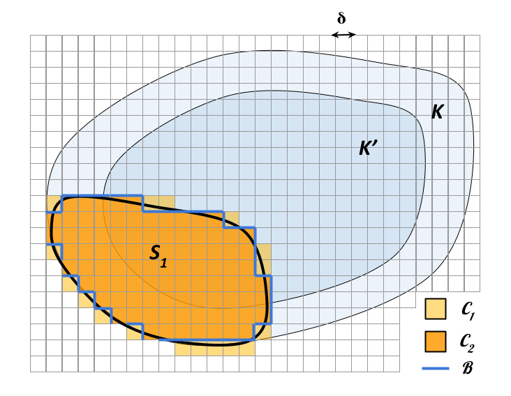
Figure 2: Illustration of the isoperimetry proof. $S_{1}$ is bounded by the thick black curve. $\mathcal{C}_{1}$ is shaded in yellow, $\mathcal{C}_{2}$ is shaded in orange, and $\mathcal{B}$ is colored blue.

Depending on whether most of the volume $S_{1}$ is contained in $\mathcal{C}_{1}$ or $\mathcal{C}_{2}$, there are two possibilities:

Case 1: If $\mathrm{vol}(\mu({\cal C}_{1})\cap S_{1})\geq\mathrm{vol}(S_{1})/2$, i.e., at least half of $\mathrm{vol}(S_{1})$ resides in cubes in ${\cal C}_{1}$, then we apply Lemma 1 to every cube in $\mathcal{C}_{1}$ individually to bound $\mathrm{vol}(S_{3})$. However, $K$ might not completely contain the cubes in $\mathcal{C}_{1}$, so before using the cube isoperimetry, we move to the contracted body $K^{\prime}$. Let

$$\mathcal{C}_{1}^{\prime}=\{c\in{\cal C}_{1}:c\cap K^{\prime}\neq\emptyset\},$$

i.e., $\mathcal{C}_{1}^{\prime}$ is the subset of cubes in $\mathcal{C}_{1}$ that intersect $K^{\prime}$. By our choice of $\alpha$, $\mu({\cal C}_{1}^{\prime})\subseteq K$. Using inequality (4) on $\mu({\cal C}_{1})\cap S_{1}$ gives

$$\mathrm{vol}(\mu({\cal C}_{1}^{\prime})\cap S_{1})\geq\mathrm{vol}(\mu({\cal C}_{1})\cap S_{1}\cap K^{\prime})\geq\mathrm{vol}(\mu({\cal C}_{1})\cap S_{1})-\frac{\varepsilon}{2}\cdot\mathrm{vol}(K).$$ (5)

Now consider a cube $c$ in ${\cal C}_{1}^{\prime}$. Using Lemma 2 on $c$,

$$\mathrm{vol}(S_{3}\cap c)\geq\psi_{c}\cdot\frac{\mathrm{vol}(S_{1}\cap c)}{4}.$$ (6)

Summing (6) over every cube in ${\cal C}_{1}^{\prime}$, we get

$$\mathrm{vol}(S_{3}) \geq\frac{\psi_{c}}{4}\cdot\sum_{c\in{\cal C}_{1}^{\prime}}\mathrm{vol}(c\cap S_{1})=\frac{\psi_{c}}{4}\cdot\mathrm{vol}(\mu({\cal C}_{1}^{\prime})\cap S_{1})$$

$$\geq\frac{\psi_{c}}{4}\cdot\left(\mathrm{vol}(\mu({\cal C}_{1})\cap S_{1})-\frac{\varepsilon}{2}\cdot\mathrm{vol}(K)\right)$$ (by inequality (5))

$$\geq\frac{\psi_{c}}{4}\cdot\left(\frac{1}{2}\cdot\mathrm{vol}(S_{1})-\frac{\varepsilon}{2}\cdot\mathrm{vol}(K)\right) \mathrm{vol}(\mu({\cal C}_{1})\cap S_{1})\geq\mathrm{vol}(S_{1})/2$$ (since )

$$=\frac{\psi_{c}}{8}\cdot\left(\mathrm{vol}(S_{1})-\varepsilon\cdot\mathrm{vol}(K)\right).$$

Case 2: If $\mathrm{vol}(\mu({\cal C}_{1})\cap S_{1})<\frac{1}{2}\cdot\mathrm{vol}(S_{1})$, then $\mathrm{vol}(\mu({\cal C}_{2})\cap S_{1})\geq\frac{1}{2}\cdot\mathrm{vol}(S_{1})$. Let $\mathcal{B}$ be the set of facets of the grid-cubes that intersect $\partial_{K}(\mu({\cal C}_{2})$. Since ${\cal C}_{2}$ is a set of axis-aligned $n$-dimensional cubes, $\mathcal{B}$ is a set of axis-aligned $(n-1)$-dimensional cubes. Consider a facet $f$ in $\mathcal{B}$ with normal axis $e_{i}$, and let $f_{1}$ be the grid-cube that is adjacent to $f$ and not in ${\cal C}_{2}$, and $f_{2}$ be the grid-cube that is adjacent to $f$ an in ${\cal C}_{2}$.

Let $\pi(f)$ denote the projection of $S_{1}\cap f_{2}$ on $f$, i.e.,

$$\pi(f)=\{x\in f:\exists y\in S_{1}\cap f_{2}\;\text{ s.t. }\;x_{j}=y_{j},\;\forall j\in[n]\backslash\{i\}\}.$$

and let $\mathcal{E}(f)$ denote the extension of this projection along the $e_{i}$-axis in $f_{1}$, i.e.,

$$\mathcal{E}(f)=\{x\in f_{1}:\exists y\in\pi(f)\;\text{ s.t. }\;x_{j}=y_{j},\;\forall j\in[n]\backslash\{i\}\}.$$

Then $S_{2}\cap\mathcal{E}(f)=\emptyset$ as every point in $\mathcal{E}(f)$ is reachable from a point in $S_{1}$ along $e_{i}$ and therefore cannot be in $S_{2}$. Because the grid size is $\delta$, $\mathrm{vol}_{n-1}(f)\cdot\delta=\mathrm{vol}(f_{1})=\mathrm{vol}(f_{2})$.

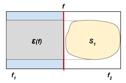
Figure 3: Figure illustrating $\mathcal{E}(f)$ for a facet $f\in\mathcal{B}$. $f$ is represented by the red line. $f_{1}$ is shaded in blue, $f_{2}$ is shaded in white, $S_{1}\cap f_{2}$ is shaded in yellow, and $\mathcal{E}(f)$ is shaded in gray.

$$\mathrm{vol}_{n-1}(\pi(f))\cdot\delta \geq\mathrm{vol}(S_{1}\cap f_{2})\geq\frac{2}{3}\cdot\mathrm{vol}(f_{2}) f_{2}\in\mathcal{C}_{2}$$ (since )

$$\Rightarrow\mathrm{vol}_{n-1}(\pi(f)) \geq\frac{2}{3}\cdot\frac{\mathrm{vol}(f_{2})}{\delta}=\frac{2}{3}\cdot\mathrm{vol}_{n-1}(f).$$

This gives

$$\mathrm{vol}(\mathcal{E}(f))\geq\delta\cdot\mathrm{vol}_{n-1}(\pi(f))\geq\frac{2}{3}\cdot\delta\cdot\mathrm{vol}_{n-1}(f).$$ (7)

Since $\mathcal{E}(f)$ does not contain $S_{2}$, it can contain $S_{1}$ and $S_{3}$. If $\mathcal{E}(f)$ does not contain $S_{1}$, then $\mathcal{E}(f)\subseteq S_{3}$ and we can add the mass from (7) to $S_{3}$. Otherwise $f_{1}\in\mathcal{C}_{1}$, and there are 2 possibilities:

• $\mathrm{vol}(S_{1}\cap f_{1})\leq\mathrm{vol}(f_{1})/3$: We can simply subtract this volume from $\mathrm{vol}(\mathcal{E}(f))$ to get

  $$\mathrm{vol}(S_{3}\cap f_{1}) \geq\mathrm{vol}(\mathcal{E}(f))-\mathrm{vol}(S_{1}\cap f_{1})$$

  $$\geq\frac{2}{3}\cdot\delta\cdot\mathrm{vol}_{n-1}(f)-\frac{1}{3}\cdot\mathrm{vol}(f_{1})=\frac{\delta}{3}\cdot\mathrm{vol}_{n-1}(f).$$

• $\frac{1}{3}\cdot\mathrm{vol}(f_{1})<\mathrm{vol}(S_{1}\cap f_{1})\leq\frac{2}{3}\cdot\mathrm{vol}(f_{1})$: Since $f_{1}\in\mathcal{C}_{1}^{\prime}$, using Lemma 2 on $f_{1}$, we get

  $$\mathrm{vol}(S_{3}\cap f_{1})\geq\psi_{c}\cdot\frac{\mathrm{vol}(S_{1}\cap f_{1})}{4}\geq\frac{\psi_{c}}{12}\cdot\mathrm{vol}(f_{1})=\frac{\psi_{c}}{12}\cdot\delta\cdot\mathrm{vol}_{n-1}(f).$$

So, for every facet $f\in\mathcal{B}$,

$$\mathrm{vol}(S_{3}\cap\mathcal{E}(f))\geq\min\left\{\frac{\psi_{c}}{12},\frac{1}{3}\right\}\cdot\delta\cdot\mathrm{vol}_{n-1}(f)=\frac{\psi_{c}}{12}\cdot\delta\cdot\mathrm{vol}_{n-1}(f).$$ (8)

Since an $n$-dimensional cube has $2n$ facets, it can contribute to the extension of a facet at most $2n$ times. Therefore, every facet on the boundary $\mathcal{B}$ contributes at least $\frac{1}{2n}\cdot\frac{\psi_{c}}{12}\cdot\delta\cdot\mathrm{vol}_{n-1}(f)$ to $\mathrm{vol}(S_{3})$. However, $f_{1}$ (and $\mathcal{E}(f)$) might not be fully contained in $K$. So we again move to the contraction $K^{\prime}$. Let

$$\mathcal{C}_{2}^{\prime}=\{c\in{\cal C}_{2}:c\cap K^{\prime}\neq\emptyset\}.$$

Our choice of $\alpha$ ensures that every cube in $\mathcal{C}_{2}^{\prime}$ and all the cubes that are adjacent to a cube in $\mathcal{C}_{2}^{\prime}$ are fully contained in $K$. Let $I=K^{\prime}\cap\mu({\cal C}_{2})$. Let $\mathcal{B}^{\prime}$ be the set of facets of grid-cubes that intersect $\partial_{K^{\prime}}(I)$, the internal boundary of $I$ relative to $K^{\prime}$.

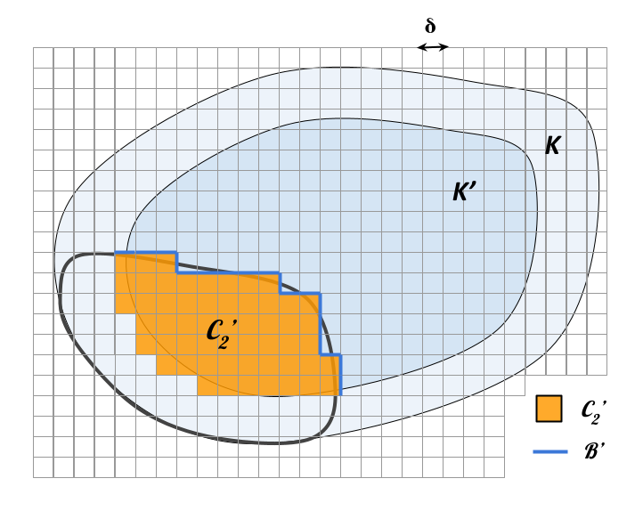
Figure 4: Illustration of $\mathcal{B}^{\prime}$ and $\mathcal{C}_{2}^{\prime}$ for the same convex body $K$ and subset $S_{1}$ as figure 2. Note that $\mathcal{B}^{\prime}\subseteq\mathcal{B}$ and all the cubes adjacent to any facet in $\mathcal{B}^{\prime}$ are completely contained in $K$.

Then $\mathcal{B}^{\prime}\subseteq\mathcal{B}$. To see this, consider a facet $f\in\mathcal{B}^{\prime}$. Let $f_{1},f_{2}$ be the grid-cubes adjacent to $f$ such that $f_{2}$ is fully contained in $I$. Because $f$ intersects the internal boundary of $I$ with respect to $K^{\prime}$, $f_{1}$ cannot be fully contained in $I$. Since $f_{1}$ has a neighbor (namely $f_{2}$) which intersects $K^{\prime}$, $f_{1}\subset K^{\prime}$. If $f_{1}\in\mathcal{C}_{2}$, then by definition $f_{1}\subset I$, which contradicts the fact that $f$ lies on the boundary of $I$. Therefore, $f_{1}\notin\mathcal{C}_{2}$, and as a result $f$ lies on the boundary of $\mathcal{C}_{2}$, i.e., $f\in\mathcal{B}$.

Therefore using (8), every facet $f\in\mathcal{B}^{\prime}$ contributes at least

$$\frac{1}{2n}\cdot\frac{\psi_{c}}{12}\cdot\delta\cdot\mathrm{vol}_{n-1}(f)$$

to $\mathrm{vol}(S_{3})$. Summing this up over $\mathcal{B}^{\prime}$,

$$\mathrm{vol}(S_{3})\geq\frac{1}{2n}\cdot\frac{\psi_{c}}{12}\cdot\delta\cdot\sum_{f\in\mathcal{B}^{\prime}}\mathrm{vol}_{n-1}(f)\geq\frac{\delta\cdot\psi_{c}}{24n}\cdot\mathrm{vol}_{n-1}\left(\partial_{K^{\prime}}(I)\right).$$ (9)

Using Lemma 3 on $I$ in $K^{\prime}$,

$$\mathrm{vol}_{n-1}\left(\partial_{K^{\prime}}(I)\right)\geq\frac{\ln{2}}{R}\cdot\min\left\{\mathrm{vol}\left(I\right),\mathrm{vol}\left(K^{\prime}\backslash I\right)\right\}.$$ (10)

Using inequality (4) on $I$,

$$\mathrm{vol}(I) =\mathrm{vol}(K^{\prime}\cap\mu(\mathcal{C}_{2}))\geq\mathrm{vol}(\mu(\mathcal{C}_{2}))-\frac{\varepsilon}{2}\cdot\mathrm{vol}(K)$$

$$\geq\frac{1}{2}\cdot(\mathrm{vol}(S_{1})-\varepsilon\cdot\mathrm{vol}(K)),$$ (11)

where the last inequality follows from $\mathrm{vol}(\mu({\cal C}_{2})\cap S_{1})\geq\frac{1}{2}\cdot\mathrm{vol}(S_{1})$. On the other hand, since $I\subseteq\mathcal{C}_{2}^{\prime}$,

$$\mathrm{vol}(I)\leq\mathrm{vol}\left(\mu({\cal C}_{2}^{\prime})\right)\leq\frac{3}{2}\cdot\mathrm{vol}\left(S_{1}\cap\mu({\cal C}_{2}^{\prime})\right)\leq\frac{3}{4}\cdot\mathrm{vol}\left(K\right),$$ (12)

where the second inequality is because $S_{1}$ occupies at least $\frac{2}{3}$ of every cube in $\mathcal{C}_{2}^{\prime}$. Therefore,

$$\mathrm{vol}(K^{\prime}\backslash I) \geq\mathrm{vol}(K^{\prime})-\frac{3}{4}\cdot\mathrm{vol}(K)\geq\left(1-\frac{\varepsilon}{2}-\frac{3}{4}\right)\cdot\mathrm{vol}(K)$$

$$\geq\frac{\mathrm{vol}(K)}{4}-\frac{\varepsilon}{2}\cdot\mathrm{vol}(K)$$

$$\geq\frac{1}{2}\cdot\left(\mathrm{vol}(S_{1})-\varepsilon\cdot\mathrm{vol}(K)\right),$$ (13)

where the last inequality uses the fact that $\mathrm{vol}(S_{1})\leq\frac{1}{2}\cdot\mathrm{vol}(K)$. Combining inequalities (10), (11), and (13), we get

$$\mathrm{vol}_{n-1}\left(\partial_{K^{\prime}}(I)\right) \geq\frac{\ln{2}}{R}\cdot\frac{1}{2}\cdot\left(\mathrm{vol}(S_{1})-\varepsilon\cdot\mathrm{vol}(K)\right).$$ (14)

Plugging the bound from inequality (14) into inequality (9) gives

$$\mathrm{vol}(S_{3}) \geq\frac{\delta\cdot\psi_{c}}{24n}\cdot\mathrm{vol}_{n-1}(\partial_{K^{\prime}}(I))$$

$$\geq\frac{\delta\cdot\psi_{c}\cdot\ln{2}}{48Rn}\cdot\left(\mathrm{vol}(S_{1})-\varepsilon\cdot\mathrm{vol}(K)\right)$$

Using $\delta=\frac{\alpha}{4\sqrt{n}}=\frac{\varepsilon}{8n\sqrt{n}}$ and $\psi_{c}=\frac{\ln{2}}{n}$, we have

$$\mathrm{vol}(S_{3})\geq\frac{\varepsilon}{800\cdot Rn^{3.5}}\cdot\left(\mathrm{vol}(S_{1})-\varepsilon\cdot\mathrm{vol}(K)\right).\qed$$

3 Conductance

In this section, we bound the $s$-conductance of CHAR. The following simple lemma lets us reduce the $s$-conductance of $K$ to the isoperimetry of axis-disjoint subsets of $K$.

Lemma 4.

Let $S_{1}\subseteq K$ be a measurable subset of $K$ and $S_{2}=K\backslash S_{1}$. Let $S_{1}^{\prime}=\{x\in S_{1}:P_{x}(S_{2})<\frac{1}{2n}\}$ and $S_{2}^{\prime}=\{x\in S_{2}:P_{x}(S_{1})<\frac{1}{2n}\}$. Then $S_{1}^{\prime}$ and $S_{2}^{\prime}$ are axis disjoint.

Proof.

For the sake of contradiction, assume that $S_{1}^{\prime}$ and $S_{2}^{\prime}$ are not axis-disjoint. Then there exists an axis-parallel line, $\ell$, passing through both $S_{1}^{\prime}$ and $S_{2}^{\prime}$.

Let $x\in S_{1}^{\prime}\cap\ell$ and $y\in S_{2}^{\prime}\cap\ell$. From the definition of $S_{1}^{\prime}$ and $S_{2}^{\prime}$,

$$\frac{1}{n}\dfrac{\text{\text{len}}(\ell\cap S_{2})}{\text{\text{len}}(\ell\cap K)} \leq P_{x}(S_{2})\leq\frac{1}{2n},\;\text{and}$$ (15)

$$\frac{1}{n}\dfrac{\text{\text{len}}(\ell\cap S_{1})}{\text{\text{len}}(\ell\cap K)} \leq P_{y}(S_{1})\leq\frac{1}{2n}\;.$$ (16)

Adding (15) and (16) implies that

$$\text{\text{len}}(\ell\cap S_{2})+\text{\text{len}}(\ell\cap S_{1})<\text{\text{len}}(\ell\cap K),$$

which is a contradiction. Therefore, $S_{1}^{\prime}$ and $S_{2}^{\prime}$ are axis-disjoint. ∎

Theorem 4.

Let $K$ be a convex body in $\mathbb{\mathbb{R}}^{n}$ containing a unit ball with $R^{2}=\mathbb{E}_{K}(\left\|x-z_{K}\right\|^{2})$ where $z_{K}$ is the centroid of $K$. Then the $s$-conductance of Coordinate Hit-and-Run in $K$ is at least $\dfrac{s}{128\cdot 10^{2}\cdot Rn^{4.5}}$.

Proof.

Let $S_{1}\subseteq K$ be a measurable subset of $K$ with $s<\pi_{K}(S_{1})\leq 1/2$ and let $S_{2}=K\backslash S_{1}$. Let

$$S_{1}^{\prime}=\{x\in S_{1}:P_{x}(S_{2})<\frac{1}{2n}\}\quad\text{ and }\quad S_{2}^{\prime}=\{x\in S_{2}:P_{x}(S_{1})<\frac{1}{2n}\}.$$

The ergodic flow of $S_{1}$ is given by

$$p(S_{1}) =\int_{x\in S_{1}}P_{x}(S_{2})\;{d\pi_{K}(x)}$$

$$=\int_{x\in S_{1}^{\prime}}P_{x}(S_{2})\;d\pi_{K}(x)+\int_{x\in S_{1}\backslash S_{1}^{\prime}}P_{x}(S_{2})\;d\pi_{K}(x).$$

Since $\int_{x\in S_{1}\backslash S_{1}^{\prime}}P_{x}(S_{2})\;d\pi_{K}(x)\geq\mathrm{vol}(S_{1}\backslash S_{1}^{\prime})/2n$, we get

$$p(S_{1})\geq\int_{x\in S_{1}\backslash S_{1}^{\prime}}P_{x}(S_{2})\;d\pi_{K}(x)\geq\frac{\mathrm{vol}(S_{1}\backslash S_{1}^{\prime})}{2n\cdot\mathrm{vol}(K)}\;.$$ (17)

We can also expand the ergodic flow of $S_{1}$ as

$$p(S_{1})=\int_{x\in S_{1}}P_{x}(S_{2}) \;d\pi_{K}(x)\geq\int_{x\in S_{1}}P_{x}(S_{2}\backslash S_{2}^{\prime})\;d\pi_{K}(x)$$

$$\stackrel{{\scriptstyle(1)}}{{=}}\int_{y\in S_{2}\backslash S_{2}^{\prime}}P_{y}(S_{1})\;d\pi_{K}(y)\geq\frac{\mathrm{vol}(S_{2}\backslash S_{2}^{\prime})}{2n\cdot\mathrm{vol}(K)}\;,$$ (18)

where (1) follows from time-reversibility of the Markov chain.

If $\mathrm{vol}(S_{1}^{\prime})<\mathrm{vol}(S_{1})/2$, then by (17),

$$p(S_{1})\geq\frac{\mathrm{vol}(S_{1})}{4n\cdot\mathrm{vol}(K)}=\frac{\pi_{K}(S)}{4n}\;.$$

This implies $\phi_{s}(S_{1})\geq\frac{1}{4n}$. Similarly, if $\mathrm{vol}(S_{2}^{\prime})<\mathrm{vol}(S_{2})/2$, then by (18),

$$p(S_{1})\geq\frac{\mathrm{vol}(S_{2})}{4n\cdot\mathrm{vol}(K)}\geq\frac{\mathrm{vol}(S_{1})}{4n\cdot\mathrm{vol}(K)}=\frac{\pi_{K}(S)}{4n}\;.$$

This also implies $\phi_{s}(S_{1})\geq\frac{1}{4n}$.

So, assume that $\mathrm{vol}(S_{1}^{\prime})\geq\mathrm{vol}(S_{1})/2$ and $\mathrm{vol}(S_{2}^{\prime})\geq\mathrm{vol}(S_{2})/2$. Let $S_{3}^{\prime}=K\backslash\{S_{1}^{\prime}\cup S_{2}^{\prime}\}$. Lemma 4 implies that $S_{1}^{\prime}$ and $S_{2}^{\prime}$ are axis-disjoint. Thus, using Theorem 2 with $\varepsilon=s/2$, we get

$$\mathrm{vol}(S_{3}^{\prime})\geq s\cdot\psi\cdot\left(\min\{\mathrm{vol}(S_{1}^{\prime}),\mathrm{vol}(S_{2}^{\prime})\}-\frac{s}{2}\cdot\mathrm{vol}(K)\right),$$ (19)

where $\psi=1/(1600\cdot n^{3.5}R)$.

Adding (17) and (18),

$$p(S_{1}) \geq\frac{1}{2}\cdot\left(\frac{\mathrm{vol}(S_{1}\backslash S_{1}^{\prime})}{2n\cdot\mathrm{vol}(K)}+\frac{\mathrm{vol}(S_{2}\backslash S_{2}^{\prime})}{2n\cdot\mathrm{vol}(K)}\right)=\frac{\mathrm{vol}(S_{3}^{\prime})}{4n\cdot\mathrm{vol}(K)}$$

$$\geq\frac{s\cdot\psi}{4n\cdot\mathrm{vol}(K)}\cdot\left(\min\{\mathrm{vol}(S_{1}^{\prime}),\mathrm{vol}(S_{2}^{\prime})\}-\frac{s}{2}\cdot\mathrm{vol}(K)\right)$$ (from (19))

$$\geq\frac{s\cdot\psi}{8n\cdot\mathrm{vol}(K)}\cdot\left(\min\{\mathrm{vol}(S_{1}),\mathrm{vol}(S_{2})\}-s\cdot\mathrm{vol}(K)\right)$$

$$\geq\frac{s\cdot\psi}{8n\cdot\mathrm{vol}(K)}\cdot\left(\mathrm{vol}(S_{1})-s\cdot\mathrm{vol}(K)\right)=\frac{s\cdot\psi}{8n}\cdot\left(\pi_{K}(S_{1})-s\right).$$

So, for any $S_{1}\subseteq K$ with $s<\pi_{K}(S_{1})\leq 1/2$, we get

$$\frac{p(S_{1})}{\pi_{K}(S_{1})-s}\geq\frac{s\cdot\psi}{8n}.$$

Thus, the $s$-conductance of the CHAR, $\phi_{s}$, is at least

$$\phi_{s}\geq\frac{s\cdot\psi}{8n}=\frac{s}{128\cdot 10^{2}\cdot Rn^{4.5}}.\qed$$

Proof of Theorem 1.

For a convex body $K$, let $\pi_{0}$ be the starting distribution of CHAR such that $\pi_{0}$ is $M$-warm with respect to $\pi_{K}$. Let $\pi_{t}$ be the distribution after $t$ steps of CHAR. Using Theorem 3 with $s=\frac{\varepsilon}{2M}$, we get

$$H_{s}\leq\frac{\varepsilon}{2}\quad\text{and}\quad d_{TV}(\pi_{t},\pi_{K})\leq\frac{\varepsilon}{2}+M\left(1-\frac{\phi_{s}^{2}}{2}\right)^{t}.$$

The above inequality, along with Theorem 4, implies that

$$t=\frac{4}{\phi_{s}^{2}}\log\frac{2M}{\varepsilon}<7\cdot 10^{4}\cdot\frac{M^{2}R^{2}n^{9}}{\varepsilon^{2}}\log\frac{2M}{\varepsilon}$$

steps of the CHAR suffice to ensure $d_{TV}(\pi_{t},\pi_{K})\leq\varepsilon$. ∎

4 Lower bound

Theorem 5.

There exists a convex body $K\in\mathbb{R}^{n}$ containing a unit ball with diameter $D$, such that the conductance of CHAR on $K$ is $O(1/n^{1.5}D)$.

We construct a convex body $K\in\mathbb{R}^{n}$ containing a unit ball such that $K$ is a skew-cylinder along the $e_{1}$ axis whose cross-sections are $(n-1)$-dimensional unit balls. The skewness of the body forces CHAR to take small steps in the $e_{1}$ direction.

Formally, let $B(x)$ be an $(n-1)$-dimensional unit ball centered at $(x,0,\ldots,0)$. The convex body $K$ is defined as

$$K=\{x\in\mathbb{R}^{n}:0\leq x_{1}\leq D,\;(x_{2},\ldots,x_{n})\in B(x_{1})\}.$$

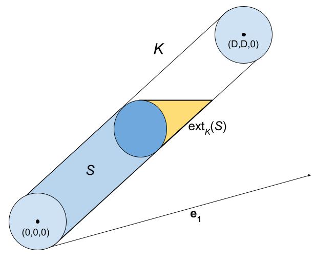
Figure 5: The lower bound construction in 3 dimensions. $S$ is shaded in blue. The extension of $S$ along $e_{1}$ is shaded in yellow. To escape $S$, Coordinate Hit-and-Run needs to move along the $e_{1}$ axis. However, the skewness of $K$ forces the step size along $e_{1}$ to be small.

Let $d=D/2$ and let $S=\{x\in K:x_{1}\leq d\}$. Then, we claim that $\phi(S)$ is $O\left(1/n^{1.5}D\right)$. Before proving this claim, we define axis-parallel extensions of subsets of convex bodies.

Definition 5 (Axis-parallel Extension).

For a convex body $K$ in $\mathbb{R}^{n}$ and a measurable subset $S\subseteq K$, the axis-parallel extension of $S$ in $K$, denoted by $\text{ext}_{K}(S)$ is defined as

$$\mathrm{ext}_{K}(S)=\{x\in K\backslash S:\exists y\in S\text{ such that }|\{i\in[n]:x_{i}=y_{i}\}|=n-1\}.$$

In other words, $\text{ext}_{K}(S)$ is the set of points in $K\backslash S$ obtained by changing exactly $1$ coordinate from a point in $S$.

We will first bound the volume of $\mathrm{ext}_{K}(S)$ and then use it to bound the conductance of CHAR on $K$.

Lemma 5.

The volume of the extension of $S$ in $K$ is at most

$$\mathrm{vol}(\mathrm{ext}_{K}(S))\leq\frac{40}{\sqrt{n}D}\cdot\mathrm{vol}(S).$$

Proof.

The extension of $S$ goes beyond $S$ only along the $e_{1}$ axis, and

$$\mathrm{ext}_{K}(S)=\{x\in K:x_{1}\in(d,d+1],\;(x_{2},\ldots,x_{n})\in B(d)\cap B(x_{1})\}.$$

Each $(n-1)$-dimensional slice of $\mathrm{ext}_{K}(S)$ is the intersection of two $(n-1)$-dimensional unit balls. This gives

$$\mathrm{vol}(\mathrm{ext}_{K}(S)) =\int_{t=0}^{1}\mathrm{vol}(B(d)\cap B(d+t))dt.$$

Figure 6: $B(d+t)\cap B(t)$

Note that $\mathrm{vol}(B(d)\cap B(d+t))$ is equal to twice the volume of spherical cap at distance $t/2$ from the center of an $(n-1)$ unit ball. By [26], the volume of a spherical cap at distance $t$ from the center of an $(n-1)$-dimensional unit ball, $C_{n-1}$, is at most $e^{-\frac{nt^{2}}{2}}\cdot\mathrm{vol}(C_{n-1})$.

Thus $\mathrm{vol}(B(d)\cap B(d+t))\leq e^{-\frac{nt^{2}}{8}}\cdot\mathrm{vol}_{n-1}(B(d))$, and

$$\mathrm{vol}(\mathrm{ext}_{K}(S)) =\int_{t=0}^{1}\mathrm{vol}(B(d)\cap B(d+t))dt$$

$$\leq 2\cdot\int_{t=0}^{\infty}e^{-\frac{nt^{2}}{8}}\cdot\mathrm{vol}_{n-1}(B(d))dt\leq\frac{20}{\sqrt{n}}\cdot\mathrm{vol}_{n-1}(B(d)).$$

Since $\mathrm{vol}(S)=\frac{D}{2}\cdot\mathrm{vol}_{n-1}(B(d))$, we have $\mathrm{vol}(\mathrm{ext}_{K}(S))\leq\frac{40}{\sqrt{n}D}\cdot\mathrm{vol}(S)$. ∎

Lemma 6.

The conductance of Coordinate Hit-and-Run on $K$ is $O(1/n^{1.5}D)$.

Proof.

The only points in $S$ with non-zero probability of escaping in one step are

$$S_{1}=\left\{x:d-1\leq x_{1}\leq d,\;(x_{2},\ldots,x_{n})\in B(d)\cap B(x_{1})\right\}.$$

Any point in $S_{1}$ can move out of $S$ in one step of CHAR if only if the first coordinate is selected for re-sampling. Therefore, for any $x\in S_{1}$,

$$P_{x}(K\backslash S)\leq 1/n.$$

By symmetry, $\mathrm{vol}(S_{1})=\mathrm{vol}(\mathrm{ext}_{K}(S))\leq\frac{40}{\sqrt{n}D}\cdot\mathrm{vol}(S)$. Therefore,

$$p(S)=\int_{S}P_{x}(K\backslash S) \;d\pi_{K}(x)=\int_{S_{1}}P_{x}(K\backslash S)\;d\pi_{K}(x)$$

$$\leq\frac{1}{n}\cdot\frac{\mathrm{vol}(S_{1})}{\mathrm{vol}(K)}\leq\frac{1}{n}\cdot\frac{40}{\sqrt{n}D}\cdot\pi_{K}(S).$$

Therefore, $\phi(S)\leq 40/(n^{1.5}D)$, and the conductance of CHAR in $K$, $\phi$, is at most $O(1/n^{1.5}D)$. ∎

We expect that this translates to a lower bound of $\Omega^{*}(n^{3}D^{2})$ on the mixing rate even from a warm start. Even though this is worse than the $O^{*}(n^{2}D^{2})$ mixing rate of Hit-and-Run, it is an interesting open problem to determine the precise mixing rate of CHAR.

Acknoledgements: This work was supported in part by NSF awards DMS-1839323, CCF-1909756 and CCF-2007443. The authors thank Ben Cousins for helpful discussions.

References

- [1] Andersen, H.C., Diaconis, P.: Hit and run as a unifying device. Journal de la société française de statistique 148(4), 5–28 (2007)
- [2] Boneh, A.: Preduce — a probabilistic algorithm identifying redundancy by a random feasible point generator (rfpg). In: Redundancy in Mathematical Programming, pp. 108–134. Springer Berlin Heidelberg, Berlin, Heidelberg (1983)
-
[3]
Cousins, B., Vempala, S.: Volume computation of convex bodies.
MATLAB File Exchange (2013).
Http://www.mathworks.com/matlabcentral/fileexchange/
43596-volume-computation-of-convex-bodies - [4] Cousins, B., Vempala, S.: Bypassing KLS: Gaussian cooling and an volume algorithm. In: STOC, pp. 539–548 (2015)
- [5] Cousins, B., Vempala, S.: A practical volume algorithm. Mathematical Programming Computation 8(2), 133–160 (2016)
- [6] Diaconis, P., Khare, K., Saloff-Coste, L.: Gibbs sampling, conjugate priors and coupling. Sankhya A 72(1), 136–169 (2010)
- [7] Diaconis, P., Lebeau, G., Michel, L.: Gibbs/metropolis algorithms on a convex polytope. Mathematische Zeitschrift 272(1-2), 109–129 (2012)
- [8] Emiris, I.Z., Fisikopoulos, V.: Efficient random-walk methods for approximating polytope volume. In: Proceedings of the thirtieth annual symposium on Computational geometry, pp. 318–327 (2014)
- [9] Finkel, J.R., Grenager, T., Manning, C.D.: Incorporating non-local information into information extraction systems by gibbs sampling. In: Proceedings of the 43rd Annual Meeting of the Association for Computational Linguistics (ACL’05), pp. 363–370 (2005)
- [10] Geman, S., Geman, D.: Stochastic relaxation, gibbs distributions, and the bayesian restoration of images. IEEE Trans. Pattern Anal. Mach. Intell. 6(6), 721–741 (1984). DOI 10.1109/TPAMI.1984.4767596. URL https://doi.org/10.1109/TPAMI.1984.4767596
- [11] George, E.I., McCulloch, R.E.: Variable selection via gibbs sampling. Journal of the American Statistical Association 88(423), 881–889 (1993)
- [12] Kannan, R.: Rapid mixing in markov chains. arXiv preprint math/0304470 (2003)
- [13] Kannan, R., Lovász, L., Simonovits, M.: Isoperimetric problems for convex bodies and a localization lemma. Discrete & Computational Geometry 13, 541–559 (1995)
- [14] Kannan, R., Lovász, L., Simonovits, M.: Random walks and an volume algorithm for convex bodies. Random Structures and Algorithms 11, 1–50 (1997)
- [15] Lee, Y.T., Vempala, S.S.: Eldan’s stochastic localization and the KLS hyperplane conjecture: An improved lower bound for expansion. In: Proc. of IEEE FOCS (2017)
- [16] Loomis, L.H., Whitney, H., et al.: An inequality related to the isoperimetric inequality. Bulletin of the American Mathematical Society 55(10), 961–962 (1949)
- [17] Lovász, L.: How to compute the volume? Jber. d. Dt. Math.-Verein, Jubiläumstagung 1990 pp. 138–151 (1990)
- [18] Lovász, L.: Hit-and-run mixes fast. Math. Prog. 86, 443–461 (1998)
- [19] Lovász, L., Simonovits, M.: Random walks in a convex body and an improved volume algorithm. In: Random Structures and Alg., vol. 4, pp. 359–412 (1993)
- [20] Lovász, L., Vempala, S.: Hit-and-run from a corner. SIAM J. Computing 35, 985–1005 (2006)
- [21] Lovász, L., Vempala, S.: Simulated annealing in convex bodies and an volume algorithm. J. Comput. Syst. Sci. 72(2), 392–417 (2006)
- [22] Lovász, L., Vempala, S.: The geometry of logconcave functions and sampling algorithms. Random Struct. Algorithms 30(3), 307–358 (2007). DOI 10.1002/rsa.v30:3
- [23] Narayanan, H., Srivastava, P.: On the mixing time of coordinate hit-and-run. arXiv preprint arXiv:2009.14004 (2020)
- [24] Sinclair, A., Jerrum, M.: Approximate counting, uniform generation and rapidly mixing Markov chains. Information and Computation 82, 93–133 (1989)
- [25] Smith, R.: Efficient Monte-Carlo procedures for generating points uniformly distributed over bounded regions. Operations Res. 32, 1296–1308 (1984)
- [26] Tkocz, T.: An upper bound for spherical caps. The American Mathematical Monthly 119(7), 606–607 (2012)
- [27] Turchin, V.: On the computation of multidimensional integrals by the monte-carlo method. Theory of Probability & Its Applications 16(4), 720–724 (1971). DOI 10.1137/1116083. URL https://doi.org/10.1137/1116083