Portfolio optimization with a
prescribed terminal wealth distribution

Abstract

This paper studies a portfolio allocation problem, where the goal is to reach a prescribed wealth distribution at final time. We study this problem with the tools of optimal mass transport. We provide a dual formulation which we solve by a gradient descent algorithm. This involves solving an associated Hamilton-Jacobi-Bellman and Fokker–Planck equation by a finite difference method. Numerical examples for various prescribed terminal distributions are given, showing that we can successfully reach attainable targets. We next consider adding consumption during the investment process, to take into account distributions that are either not attainable, or sub-optimal.

Keywords: portfolio allocation, wealth distribution target, optimal mass transport, HJB, Fokker–Planck, gradient descent

1 Introduction

Over the past decades, there has been a vast amount of research on portfolio allocation. Perhaps the most iconic result is the portfolio selection theory by Markowitz (1952), which states that investors should determine the allocation of wealth on the basis of the trade-off between return and risk. The classical objective function in a portfolio optimization problem is to maximize the expected return given variance level. However, the first and second moments of the return of a portfolio is only a simplified description of the wealth. Researchers then introduced objective functions that include more moments, such as skewness, to provide a more accurate statistic description of the distribution of the return (see, for example, Kraus and Litzenberger 1976 and Lee 1977).

The whole distribution of the portfolio wealth would provide investors a complete information, and instead of optimizing the first moments of the distribution, our paper introduces an objective function which includes a target distribution of the terminal wealth. We address the problem of controlling the portfolio allocation process to reach the prescribed terminal distribution. Of course, as we will see not all distributions are attainable.

On the one hand, this problem can be categorized as a stochastic control problem. The state variable is influenced by a process whose value is decided at any time $t\in[0,T]$, and we define such a process as a control. We can treat the portfolio allocation process as a control in the investment process. We aim to design the time path of the portfolio allocation process such that it steers the portfolio wealth from an initial state to a prescribed terminal distribution.

One the other hand, designing a continuous semimartingale having prescribed distributions at given times can be addressed with the optimal mass transport (OMT) theory. The optimal transport problem is an old problem first addressed in the work of Monge (1781), and was later revisited by Kantorovich (1942) leading to the so-called Monge–Kantorovich formulation. A comprehensive review of the extensions and applications of the Monge–Kantorovitch problem can be found in the book by Rachev and Rüschendorf (1998) and the books of Villani (2003, 2008). The original formulation of the problem looks for a map $f:X\to Y$ that pushes a distribution $\mu$ to another distribution $\nu$. Later, Benamou and Brenier (2000) reinterpreted the problem in a fluid mechanics framework, where one is not looking only for an optimal transport map, but instead for the whole trajectory of the mass distribution over time. This contribution opened the way to the problem of continuous optimal transport.

Stochastic extensions of the discrete and time continuous OMT problem have then flourished, see e.g. Mikami and Thieullen (2006), Tan et al. (2013), Mikami (2015), Henry-Labordère et al. (2016). Beyond its mathematical interest, the optimal mass transport problem has applications in many fields, in economy, meteorology, astrophysics (Brenier et al. 2003, Loeper 2006), image processing (Ferradans et al. 2014), finance (Dolinsky and Soner 2014, Henry-Labordère 2017).

The novelty of this paper is to provide a new perspective on portfolio optimization inspired by OMT. An investor must decide how to allocate her portfolio between a risky and a risk-free asset. The price of the risky asset is modelled by a semimartingale, with prescribed drift and diffusion coefficients. By controlling the portfolio allocation, she wants the distribution of the wealth to match, or be close to, a given target distribution. Depending on the risky asset diffusion coefficients, not all target distributions are attainable (think for example of too high an expected return versus variance), or optimal (one could reach a “better” distribution than the target). We consider two different approaches: either relaxing the terminal constraint by penalization, or adding a consumption process, whereby the investor can either inject or withdraw cash from the portfolio in order to reach the target.

The rest of the paper is organized as follows. In Section 2, we formulate the problem. Then we introduce the dual formulation in Section 3. In Section 4, we provide a gradient descent algorithm to solve the dual problem, and the numerical results are presented in Section 5. We give examples for general target distributions with various penalty functionals in Section 5.1. We consider the addition of consumption/cash input in Section 5.2 and Section 5.3.

2 Problem Formulation

Let $\mathcal{D}$ be a Polish space equipped with its Borel $\sigma$-algebra. We denote $C(\mathcal{D};\mathbb{R})$ the space of continuous functions on $\mathcal{D}$ with values in $\mathbb{R}$, $C_{b}(\mathcal{D};\mathbb{R})$ the space of bounded continuous functions and $C_{0}(\mathcal{D};\mathbb{R})$ the space of continuous functions, vanishing at infinity. Let $\mathcal{P}(\mathcal{D})$ be the space of Borel probability measures on $\mathcal{D}$ with a finite second moment. Denote by $\mathcal{M}(\mathcal{D};\mathbb{R})$ the space of finite signed measures on $\mathcal{D}$ with values in $\mathbb{R}$, $\mathcal{M}_{+}(\mathcal{D};\mathbb{R})\subset\mathcal{M}(\mathcal{D};\mathbb{R})$ be the subset of non-negative measures. When $\mathcal{D}$ is compact, the topological dual of $C_{b}$ is given by $C_{b}(\mathcal{D};\mathbb{R})^{*}=\mathcal{M}(\mathcal{D};\mathbb{R})$. But when $\mathcal{D}$ is non-compact, $C_{b}(\mathcal{D};\mathbb{R})^{*}$ is larger than $\mathcal{M}(\mathcal{D};\mathbb{R})$. For convenience, we often use the notation $\mathcal{E}\coloneqq[0,1]\times\mathbb{R}$. We say that a function $\phi:\mathcal{E}\rightarrow\mathbb{R}$ belongs to $C_{b}^{1,2}(\mathcal{E})$ if $\phi\in C_{b}(\mathcal{E})$ and $(\partial_{t}\phi,\partial_{x}\phi,\partial_{xx}\phi)\in C_{0}(\mathcal{E};\mathbb{R},\mathbb{R},\mathbb{R})$. Let $\mathbb{R}^{+}$ denote non-negative real numbers, and $\mathbb{S}^{d}$ denote the set of symmetric positive semidefinite matrices.

Let $\Omega\coloneqq(\omega\in C([0,1];\mathbb{R}^{d})),$ we denote by $\mathbb{F}=(\mathcal{F}_{t})_{t\in[0,1]}$ the filtration generated by the canonical process. The process $W$ is a $d$-dimensional standard Brownian motion on the filtered probability space $\left(\Omega,\mathcal{F},\mathbb{F},\mathbb{P}\right)$.

We consider a portfolio with $d$ risky assets and one risk-free asset, the risk-free interest $r$ being set to 0 for simplicity. We assume the drift $\mu:\mathcal{E}\rightarrow\mathbb{R}^{d}$ and covariance matrix $\Sigma:\mathcal{E}\rightarrow\mathbb{S}^{d}$ of the risky assets are known Markovian processes. Without loss of generality, we set the time horizon $T$ to be $1$. The price process of the risky assets is denoted by $S_{t}\in\mathbb{R}^{d}$ $(0\leq t\leq 1)$, and the $i$th element of $S_{t}$ follows the semimartingale

$$\frac{dS_{t}^{i}}{S_{t}^{i}}=\mu_{t}^{i}dt+\sum_{j=1}^{d}\sigma_{t}^{ij}dW_{t}^{j},\quad 1\leq i\leq d,$$ (1)

where $\sigma_{t}\coloneqq\Sigma_{t}^{\frac{1}{2}}\in\mathbb{R}^{d\times d}$ is the diffusion coefficient matrix.

The process $\alpha=(\alpha_{t})_{t\in[0,1]}$ is a Markovian control. For $t\in[0,1]$, the portfolio allocation strategy $\alpha_{t}\in\mathbb{R}^{d}$ represents the proportion of the total wealth invested into the $d$ risky assets, and $1-\sum_{i=1}^{d}\alpha_{t}^{i}$ is the proportion invested in the risk-free asset. We define the concept of admissible control as follows.

Definition 1.

An admissible control process $\alpha$ for the investor on $[0,1]$ is a progressively measurable process with respect to $\mathbb{F}$, taking values in a compact convex set $K\subset\mathbb{R}^{d}$. The set of all admissible $\alpha$ is compact and convex, denoted by $\mathcal{\mathcal{K}}$.

We denote by $X_{t}\in\mathbb{R}$ the portfolio wealth at time $t$. Starting from an initial wealth $x_{0}$, the wealth of the self-financing portfolio evolves as follows,

$$dX_{t} =X_{t}\alpha_{t}^{\intercal}\mu_{t}dt+X_{t}\alpha_{t}^{\intercal}\sigma_{t}dW_{t},$$ (2)

$$X_{0} =x_{0}.$$ (3)

2.1 Portfolio optimization with a prescribed terminal distribution

We denote by $\rho_{t}\coloneqq\mathbb{P}\circ X_{t}^{-1}\in\mathcal{P}(\mathbb{R})$ the distribution of $X_{t}$. In this problem, we know the initial distribution of the portfolio wealth $\rho_{0}\in\mathcal{P}(\mathbb{R})$, we are given a prescribed terminal distribution $\bar{\rho}_{1}\in\mathcal{P}(\mathbb{R})$ and a convex cost function $f(\alpha_{t}):K\rightarrow\mathbb{R}$.

With $\rho_{0}$ and a process $\alpha$, the realized terminal distribution of the portfolio wealth is $\rho_{1}\coloneqq\mathbb{P}\circ X_{1}^{-1}$ ($\rho_{1}$ is not necessarily the same as $\bar{\rho}_{1}$). We want $\rho_{1}$ to be close to our target $\bar{\rho}_{1}$, hence we introduce a functional $C(\rho_{1},\bar{\rho}_{1})$ to penalize the deviation of $\rho_{1}$ from $\bar{\rho}_{1}$. At the same time, we want to minimize the expectation of the transportation cost from $\rho_{0}$ to $\rho_{1}$. Combining the expected transportation cost and the penalty functional, our objective function is

$$\inf_{\alpha,\rho}\left\{\int_{\mathcal{E}}f(\alpha_{t})d\rho(t,x)+C(\rho_{1},\bar{\rho}_{1})\right\},$$ (4)

where the feasible $(\alpha,\rho)$ in (4) should satisfy the initial distribution

$$\rho(0,x) =\rho_{0}(x) \quad\forall x\in\mathbb{R},$$ (5)

and the Fokker–Planck equation

$$\partial_{t}\rho(t,x)+\partial_{x}(\alpha_{t}^{\intercal}\mu_{t}x\rho(t,x))-\frac{1}{2}\partial_{xx}(\alpha_{t}^{\intercal}\Sigma_{t}\alpha_{t}x^{2}\rho(t,x)) =0 \quad\forall(t,x)\in\mathcal{E}.$$ (6)

However, the feasible set for $(\alpha,\rho)$ defined by equality (6) is not convex, which means we may not be able to find the optimal solution. To address this issue, we introduce the following definition.

Definition 2.

We define maps $\tilde{B},\tilde{A}:\mathcal{E}\rightarrow\mathbb{R}$ as $\tilde{B}(t,x)\coloneqq\alpha_{t}^{\intercal}\mu_{t}x$ and $\tilde{A}(t,x)\coloneqq\alpha_{t}^{\intercal}\Sigma_{t}\alpha_{t}x^{2}$. Then define $B(t,x)\coloneqq\tilde{B}\rho$, $B\in\mathcal{M}(\mathcal{E};\mathbb{R})$ and $A(t,x)\coloneqq\tilde{A}\rho$, $A\in\mathcal{M}^{+}(\mathcal{E};\mathbb{R})$. Measures $B$ and $A$ are absolutely continuous with respect to $\rho$.

We show that $B$ and $A$ are connected in the following way:

Proposition 1.

When $d>1$ (resp. $d=1$), the necessary and sufficient condition for the existence of an $\alpha_{t}\in\mathbb{R}^{d}$ satisfying Definition 2 is $A\geq\frac{B^{2}}{\left\|\nu_{t}\right\|^{2}\rho}$ (resp. $A=\frac{B^{2}}{\left\|\nu_{t}\right\|^{2}\rho}$), where $\nu_{t}\coloneqq\Sigma_{t}^{-\frac{1}{2}}\mu_{t}$.

Proof.

See Section A.1. ∎

Using notations $\rho,B$ and $A$, the Fokker–Planck equation (6) becomes linear and the SDE of the portfolio wealth reads

$$dX_{t} =\tilde{B}(t,X_{t})dt+\tilde{A}^{\frac{1}{2}}(t,X_{t})dW_{t},$$ (7)

$$X_{0} =x_{0}.$$ (8)

From Proposition 1, at time $t$, it is possible that the optimal drift $\tilde{B}(t,x)$ is not saturated, i.e., $\tilde{B}(t,x)^{2}<\left\|\nu_{t}\right\|^{2}\tilde{A}(t,x)$. It means that the drift function in SDE (7) can be greater and eventually we can reach a better terminal wealth with a higher expectation. Then, instead of using this unsaturated drift $\tilde{B}(t,x)$ to reach the prescribed terminal distribution, we can use the drift $\tilde{B}(t,x)=\left\|\nu_{t}\right\|\sqrt{\tilde{A}}$ to attain a more ambitious distribution, and the extra part in the drift can be interpreted as cash saving. In this case, even when we have multiple assets ($d>1$) in the portfolio, optimal portfolios should lie on the curve $\tilde{B}(t,x)=\left\|\nu_{t}\right\|\sqrt{\tilde{A}}$, as in the $d=1$ case. Any portfolio lying below the curve represents a less than ideal investment because for the same level of risk (variance), we could achieve a greater return. This is consistent with the efficient frontier in modern portfolio theory (Markowitz 1952).

Now we define the concept of cash saving at time $t$ as $c_{t}\coloneqq\left\|\nu_{t}\right\|\sqrt{\tilde{A}(t,x)}-\tilde{B}(t,x)$. When the prescribed terminal distribution is not ambitious enough, to ensure we have as much cash saving as we can, we define the new feasible set as $\varPi\coloneqq\{(\rho,B,A):A\geq\frac{(B^{+})^{2}}{\left\|\nu_{t}\right\|^{2}\rho}\}$ ($B^{+}\coloneqq\max(0,B)$) and we can see the set $\varPi$ is convex. To penalize measures out of the set $\varPi$, we define a cost function $F:\mathcal{E}\times\mathbb{R}\times\mathbb{R}\rightarrow\mathbb{R}^{+}\cup\{+\infty\}$ such that

$$F\left(\frac{B}{\rho},\frac{A}{\rho}\right)=f\left(\frac{B}{\rho},\frac{A}{\rho}\right)+\delta(\rho,B,A),$$ (9)

where $f:\mathcal{E}\times\mathbb{R}\times\mathbb{R}\rightarrow\mathbb{R}^{+}$ is a convex function and $\delta(\rho,B,A)$ is a delta function defined as

$$\delta(\rho,B,A)=\begin{cases}0&\text{if }(\rho,B,A)\in\varPi,\\ +\infty&\text{otherwise}.\end{cases}$$ (10)

Now we are ready to introduce formally the problem:

Problem 1.

Starting from an initial distribution $\rho_{0}$, with a prescribed terminal distribution $\bar{\rho}_{1}$ and a cost function (9), we want to solve the infimum of the functional

$$V(\rho_{0},\bar{\rho}_{1})=\inf_{\rho,B,A}\int_{\mathcal{E}}F\left(\frac{B}{\rho},\frac{A}{\rho}\right)d\rho+C(\rho_{1},\bar{\rho}_{1})$$ (11)

over all $(\rho,B,A)\in\mathcal{M}(\mathcal{E};\mathbb{R}\times\mathbb{R}\times\mathbb{R})$ satisfying the constraints

$$\partial_{t}\rho(t,x)+\partial_{x}B(t,x)-\frac{1}{2}\partial_{xx}A(t,x)=0\quad\forall(t,x)\in\mathcal{E},$$ (12)

$$\rho(0,x)=\rho_{0}(x)\quad\forall x\in\mathbb{R}.$$ (13)

2.2 Assumptions

We make the following assumptions which will hold throughout the paper.

Assumption 1.

The probability measure $\rho_{t}$, $t\in(0,1]$ is absolutely continuous with respect to the Lebesgue measure.

Assumption 2.

The penalty functional $C(\cdot,\bar{\rho}_{1}):\mathcal{P}(\mathbb{R})\rightarrow\mathbb{R}^{+}$ is lower semi-continuous and convex. We have $C(\rho_{1},\bar{\rho}_{1})=0$ if and only if $\rho_{1}(x)=\bar{\rho}_{1}(x)$ almost everywhere.

Assumption 3.

 

1. The function $F(\frac{B}{\rho},\frac{A}{\rho})$ is non-negative, lower semi-continuous and strictly convex in $(\frac{B}{\rho},\frac{A}{\rho})$.

2. The cost function $F(\frac{B}{\rho},\frac{A}{\rho})$ is coercive in the sense that there exist constants $m>1$ and $K>0$ such that

   $$\left|\frac{B}{\rho}\right|^{m}+\left|\frac{A}{\rho}\right|^{m}\leq K\left(1+F\left(\frac{B}{\rho},\frac{A}{\rho}\right)\right),\qquad\forall(t,x)\in\mathcal{E}.$$

3. For all $(t,x)\in\mathcal{K}$, and for any $(\rho,B,A)\in\varPi$, we have

   $$\int_{\mathcal{E}}\left|F\left(\frac{B}{\rho},\frac{A}{\rho}\right)\right|d\rho<\infty,$$

   and

   $$\mathbb{E}\left[\int_{0}^{1}\left|\frac{B}{\rho}\right|^{2}+\left|\frac{A}{\rho}\right|dt\right]<\infty.$$

For simplicity, we write $F(\frac{B}{\rho},\frac{A}{\rho})\coloneqq F(t,x,\frac{B}{\rho},\frac{A}{\rho})$ if there is no ambiguity.

3 Duality

In this section, we introduce the dual problem to Problem 1, this allows us to give optimality condition for the primal problem. First of all, we find out the convex conjugate of the cost functional, which will be used in the later proof.

3.1 Convex Conjugate

Define a function $G:C_{b}(\mathcal{E};\mathbb{R}\times\mathbb{R}\times\mathbb{R})\rightarrow\mathbb{R}\cup\{+\infty\}$ as

$$G(u,b,a) =\sup_{\rho,\tilde{B},\tilde{A}}\Bigl{\{}u\rho+b\tilde{B}\rho+a\tilde{A}\rho-F(\tilde{B},\tilde{A})\rho\Bigr{\}}$$

$$=\sup_{\rho}\Bigl{\{}\rho\Bigl{[}u+\sup_{\tilde{A}\geq\frac{(\tilde{B}^{+})^{2}}{\left\|\nu_{t}\right\|^{2}}}\left(b\tilde{B}+a\tilde{A}-F(\tilde{B},\tilde{A})\right)\Bigr{]}\Bigr{\}}$$

$$=\sup_{\rho}\Bigl{\{}\rho\Bigl{[}u+F^{*}(b,a)\Bigr{]}\Bigr{\}},$$

where $F^{*}$ is the convex conjugate of $F$. Since $\rho(t,x)$ is non-negative, it is obvious that

$$G(u,b,a)=\begin{cases}0&\text{if }u+F^{*}(b,a)\leq 0\quad\forall(t,x)\in\mathcal{K},\\ +\infty&\text{otherwise}.\end{cases}$$

If we restrict the domain of its convex conjugate $G^{*}:C_{b}^{*}(\mathcal{E};\mathbb{R}\times\mathbb{R}\times\mathbb{R})\rightarrow\mathbb{R}\cup\{+\infty\}$ to $\mathcal{M}(\mathcal{E};\mathbb{R}\times\mathbb{R}\times\mathbb{R})$, then

$$G^{*}(\rho,B,A) =\sup_{(u,b,a)\in C_{b}(\mathcal{E};\mathbb{R}\times\mathbb{R}\times\mathbb{R})}\left\{u\rho+bB+aA:u+F^{*}(b,a)\leq 0\right\}.$$ (14)

Because the function to be optimized is linear and $\rho(t,x)\geq 0$, we can see the optimal $u^{*}=-F^{*}(b,a)$ in (14). With $F$ being convex and lower-semicontinuous, we have

$$G^{*}(\rho,B,A) =\sup_{(b,a)\in C_{b}(\mathcal{E};\mathbb{R}\times\mathbb{R})}\left\{-F^{*}(b,a)+b\tilde{B}+a\tilde{A}\right\}\rho$$

$$=F\left(\frac{B}{\rho},\frac{A}{\rho}\right)\rho.$$

The supremum is pointwise in time and space, and we can write

$$\int_{\mathcal{E}}F\left(\frac{B}{\rho},\frac{A}{\rho}\right)d\rho=\sup_{(u,b,a)\in C_{b}(\mathcal{E};\mathbb{R}\times\mathbb{R}\times\mathbb{R})}\Bigl{\{}\int_{\mathcal{E}}ud\rho+bdB+adA:u+F^{*}(b,a)\leq 0\Bigr{\}}.$$ (15)

3.2 Dual Problem

Now we can state our main result. A key element in the dual problem is the Hamilton–Jacobi–Bellman (HJB) equation:

$$\partial_{t}\phi+\sup_{\tilde{A}\geq\frac{(\tilde{B}^{+})^{2}}{\left\|\nu_{t}\right\|^{2}}}\Bigl{\{}\partial_{x}\phi\tilde{B}+\frac{1}{2}\partial_{xx}\phi\tilde{A}-F(\tilde{B},\tilde{A})\Bigr{\}}=0.$$ (16)

For any $\phi(t,x)\in C_{b}^{1,2}(\mathcal{E})$ solution of the HJB equation (16), Itô’s formula yields,

$$\int_{\mathbb{R}}\phi_{1}d\rho_{1}-\phi_{0}d\rho_{0} =\int_{\mathcal{E}}\left(\partial_{t}\phi+\partial_{x}\phi\tilde{B}+\frac{1}{2}\partial_{xx}\phi\tilde{A}\right)d\rho$$

$$=\int_{\mathcal{E}}\left(-F^{*}(\partial_{x}\phi,\frac{1}{2}\partial_{xx}\phi)+\partial_{x}\phi\tilde{B}+\frac{1}{2}\partial_{xx}\phi\tilde{A}\right)d\rho$$

$$\leq\int_{\mathcal{E}}F(\tilde{B},\tilde{A})d\rho.$$

Adding the penalty functional to both sides yields

$$\int_{\mathbb{R}}\phi_{1}d\rho_{1}-\int_{\mathbb{R}}\phi_{0}d\rho_{0}+C(\rho_{1},\bar{\rho}_{1}) \leq\int_{\mathcal{E}}F(\tilde{B},\tilde{A})d\rho+C(\rho_{1},\bar{\rho}_{1}).$$ (17)

Taking the infimum of the left hand side of (17) over $\rho_{1}$ and taking the infimum of the right hand side of (17) over $(\rho,B,A)$, we get

$$-C^{*}(-\phi_{1})-\int_{\mathbb{R}}\phi_{0}d\rho_{0} \leq\inf_{(\rho,B,A)\in\mathcal{M}(\mathcal{E};\mathbb{R}\times\mathbb{R}\times\mathbb{R})}\int_{\mathcal{E}}F\left(\frac{B}{\rho},\frac{A}{\rho}\right)d\rho+C(\rho_{1},\bar{\rho}_{1})$$

$$\leq V(\rho_{0},\bar{\rho}_{1}).$$

The following result shows that optimizing the left hand side yields an equality.

Theorem 1 (Duality).

When $C(\rho_{1},\bar{\rho}_{1})$ is continuous, there holds

$$V(\rho_{0},\bar{\rho}_{1}) =\sup_{\phi}\left\{-C^{*}(-\phi_{1})-\int_{\mathbb{R}}\phi_{0}d\rho_{0}\right\},$$ (18)

where the supremum is taken over all $\phi(t,x)\in C_{b}^{1,2}(\mathcal{E})$ satisfying

$$\partial_{t}\phi(t,x)+\sup_{\tilde{A}\geq\frac{(\tilde{B}^{+})^{2}}{\left\|\nu_{t}\right\|^{2}}}\left\{\partial_{x}\phi\tilde{B}+\frac{1}{2}\partial_{xx}\phi\tilde{A}-F(\tilde{B},\tilde{A})\right\} \leq 0, \forall(t,x)\in[0,1]\times\mathbb{R}.$$ (19)

Proof.

This proof is an application of the Fenchel–Rockafellar duality theorem, e.g., Brezis (2010, Theorem 1.12). From the constraint (12), we have that for all $\phi\in C_{b}^{1,2}(\mathcal{E})$,

$$\int_{\mathbb{R}}\int_{0}^{1}\phi\partial_{t}\rho+\phi\partial_{x}B-\frac{1}{2}\phi\partial_{xx}Adtdx=0.$$ (20)

Integrating by parts we obtain

$$\int_{\mathbb{R}}\phi_{1}d\rho_{1}-\phi_{0}d\rho_{0}-\int_{\mathcal{E}}\partial_{t}\phi d\rho+\partial_{x}\phi dB+\frac{1}{2}\partial_{xx}\phi dA=0.$$ (21)

Because of equation (15), we can reformulate the primal problem (11) as a saddle point problem:

$$V(\rho_{0},\bar{\rho}_{1}) =\inf_{\rho,B,A}\sup_{u+F^{*}(b,a)\leq 0}\int_{\mathcal{E}}ud\rho+bdB+adA+C(\rho_{1},\bar{\rho}_{1}).$$ (22)

Adding the Lagrangian penalty (21) to the functional (22), then Problem 1 can be written as

$$V(\rho_{0},\bar{\rho}_{1})=\inf_{\rho,B,A}\sup_{u+F^{*}(b,a)\leq 0,\phi}\int_{\mathcal{E}}ud\rho+bdB+adA+C(\rho_{1},\bar{\rho}_{1})$$

$$+\int_{\mathbb{R}}\phi_{1}d\rho_{1}-\phi_{0}d\rho_{0}-\int_{\mathcal{E}}\partial_{t}\phi d\rho+\partial_{x}\phi dB+\frac{1}{2}\partial_{xx}\phi dA.$$

We write $C^{*}(r):C_{b}(\mathbb{R};\mathbb{R})\rightarrow\mathbb{R}\cup\{+\infty\}$ for the convex conjugate of functional $C(\rho_{1},\bar{\rho}_{1})$:

$$C^{*}(r)=\sup_{\rho_{1}\geq 0}\Bigl{\{}\int_{\mathbb{R}}rd\rho_{1}-C(\rho_{1},\bar{\rho}_{1})\Bigr{\}}.$$

Here we define the functional $\alpha:C_{b}(\mathcal{E};\mathbb{R}\times\mathbb{R}\times\mathbb{R}\times\mathbb{R})\rightarrow\mathbb{R}\cup\{+\infty\}$ by

$$\alpha(u,b,a,r)=\begin{cases}C^{*}(r)&\text{ if }u+F^{*}(b,a)\leq 0,\\ +\infty&\text{ otherwise }.\end{cases}$$ (23)

Its convex conjugate $\alpha^{*}:C_{b}^{*}(\mathcal{E};\mathbb{R}\times\mathbb{R}\times\mathbb{R}\times\mathbb{R})\rightarrow\mathbb{R}\cup\{+\infty\}$ is defined as

$$\alpha^{*}(\rho,B,A,\rho_{1}) =\sup_{u+F^{*}(b,a)\leq 0,r}\int_{\mathcal{E}}ud\rho+bdB+adA+\Bigl{[}\int_{\mathbb{R}}rd\rho_{1}-C^{*}(r)\Bigr{]}.$$ (24)

If we restrict the domain to $\mathcal{M}(\mathcal{E};\mathbb{R}\times\mathbb{R}\times\mathbb{R}\times\mathbb{R})$, with (15) and Assumption 2, we have

$$\alpha^{*}(\rho,B,A,\rho_{1}) =\begin{cases}\int_{\mathcal{E}}F(\frac{B}{\rho},\frac{A}{\rho})d\rho+C(\rho_{1},\bar{\rho}_{1})&\text{if }\rho\in\mathcal{M}_{+}\text{ and }B=\tilde{B}\rho,A=\tilde{A}\rho,\\ +\infty&\text{ otherwise}.\end{cases}$$

Indeed, if $\rho$ is not positive in (24), we would let $b=a=0$ and $u=-\lambda\mathbbm{1}_{O}$ for some $O$ such that $\rho(O)<0$ and let $\lambda\rightarrow+\infty$. If $B$ or $A$ are not absolutely continuous with respect to $\rho$, we can find some $O$ such that $\rho(O)=0$ but $B(O)\neq 0$ or $A(O)\neq 0$. Then we let $u=-F^{*}(b,a)$ and $b=a=\lambda\mathbbm{1}_{O}$, and $\alpha^{*}(\rho,B,A)\geq\lambda B(O)+\lambda A(O)\rightarrow+\infty$ by letting $\lambda\rightarrow\pm\infty$ depending on the sign of $B(O)$ and $A(O)$.

Next, we say that the set $(u,b,a,r)\in C_{b}(\mathcal{E};\mathbb{R}\times\mathbb{R}\times\mathbb{R}\times\mathbb{R})$ is represented by $\phi\in C_{b}^{1,2}(\mathcal{E})$ if

$$u=-\partial_{t}\phi,\quad b=-\partial_{x}\phi,\quad a=-\frac{1}{2}\partial_{xx}\phi,\quad r=\phi_{1}.$$

Then define $\beta:C_{b}(\mathcal{E};\mathbb{R}\times\mathbb{R}\times\mathbb{R}\times\mathbb{R})\rightarrow\mathbb{R}\cup\{+\infty\}$ as follows,

$$\beta(u,b,a,r)=\begin{cases}\int_{\mathbb{R}}\phi_{0}d\rho_{0}&\text{ if }(u,b,a,r)\text{ is represented by }\phi\in C_{b}^{1,2}(\mathcal{E}),\\ +\infty\qquad&\text{ otherwise}.\end{cases}$$ (25)

Notice that $\beta$ is well-defined, indeed, it does not depend on the choice of $\phi$. If both $\phi,\psi$ represent $u,b,a,r$, then $\phi_{1}=\psi_{1}\forall x\in\mathbb{R}$, $\partial_{t}\phi(t,x)=\partial_{t}\psi(t,x)$, $\partial_{x}\phi(t,x)=\partial_{x}\psi(t,x)$, $\partial_{xx}\phi(t,x)=\partial_{xx}\psi(t,x)$ $\forall(t,x)\in\mathcal{K}$. It follows that $\phi_{0}(x)=\psi_{0}(x)$ $\forall x\in\mathbb{R}$. The set of represented functions $(u,b,a,r)$ is a linear subspace, and $\beta$ is linear with respect to $(u,b,a,r)$ in the convex set. Hence $\beta$ is convex and its convex conjugate $\beta^{*}:C_{b}^{*}(\mathcal{E};\mathbb{R}\times\mathbb{R}\times\mathbb{R}\times\mathbb{R})\rightarrow\mathbb{R}\cup\{+\infty\}$ is

$$\beta^{*}(\rho,B,A,\rho_{1})= \sup_{u,b,a,r}\int_{\mathcal{E}}ud\rho+bdB+adA+\int_{\mathbb{R}}rd\rho_{1}-\phi_{0}d\rho_{0},$$

$$\quad\text{over all }(u,b,a,r)\in C_{b}(\mathcal{E};\mathbb{R}\times\mathbb{R}\times\mathbb{R}\times\mathbb{R})\text{ represented by }\phi\in C_{b}^{1,2}(\mathcal{E}).$$

Or equivalently,

$$\beta^{*}(\rho,B,A,\rho_{1}) =\sup_{\phi}\int_{\mathcal{E}}-\partial_{t}\phi d\rho-\partial_{x}\phi dB-\frac{1}{2}\partial_{xx}\phi dA+\int_{\mathbb{R}}\phi_{1}d\rho_{1}-\phi_{0}d\rho_{0}.$$

We find that $\beta^{*}(\rho,B,A,\rho_{1})=0$ if $(\rho,B,A,\rho_{1})$ satisfies (21), and $\beta^{*}(\rho,B,A,\rho_{1})=+\infty$ otherwise.

Now we can express our objective functional $V(\rho_{0},\bar{\rho}_{1})$ as

$$V(\rho_{0},\bar{\rho}_{1}) ={\inf_{(\rho,B,A)\in\mathcal{M}(\mathcal{E};\mathbb{R}\times\mathbb{R}\times\mathbb{R})}\left\{\alpha^{*}(\rho,B,A,\rho_{1})+\beta^{*}(\rho,B,A,\rho_{1})\right\}}$$

$$={\inf_{(\rho,B,A,\rho_{1})\in\mathcal{M}(\mathcal{E};\mathbb{R}\times\mathbb{R}\times\mathbb{R}\times\mathbb{R})}\left\{\alpha^{*}(\rho,B,A,\rho_{1})+\beta^{*}(\rho,B,A,\rho_{1})\right\}}$$

$$=\inf_{(\rho,B,A,\rho_{1})\in C_{b}^{*}(\mathcal{E};\mathbb{R}\times\mathbb{R}\times\mathbb{R}\times\mathbb{R})}\left\{\alpha^{*}(\rho,B,A,\rho_{1})+\beta^{*}(\rho,B,A,\rho_{1})\right\}.$$

The second equality is because $\beta^{*}(\rho,B,A,\rho_{1})=+\infty$ if $\rho_{1}$ does not equal to $\rho(t,x)$ at time $t=1$. We prove the third equality in Section A.2.

We can let $\phi(t,x)=t$, then $u=-1,b=0,a=0,r=1$. We can see $\alpha(-1,0,0,1)=1$ and it is continuous in $(u,b,a,r)$ at this point, and $\beta(-1,0,0,1)=0$ being finite at this point. Finally, the conditions of Fenchel duality theorem in Brezis (2010, Theorem 1.12) are fulfilled, and it implies

$$V(\rho_{0},\bar{\rho}_{1}) =\inf_{(\rho,B,A,\rho_{1})\in C_{b}^{*}(\mathcal{E};\mathbb{R}\times\mathbb{R}\times\mathbb{R}\times\mathbb{R})}\left\{\alpha^{*}(\rho,B,A,\rho_{1})+\beta^{*}(\rho,B,A,\rho_{1})\right\}$$

$$=\sup_{(u,b,a,r)\in C_{b}(\mathcal{E};\mathbb{R}\times\mathbb{R}\times\mathbb{R}\times\mathbb{R})}\left\{-\alpha(-u,-b,-a,-r)-\beta(u,b,a,r)\right\},$$

over the set $(u,b,a,r)$ being represented by $\phi\in C_{b}^{1,2}(\mathcal{E})$, and satisfying $-u+F^{*}(-b,-a)\leq 0$.

Therefore we express $V(\rho_{0},\bar{\rho}_{1})$ in terms of $\phi$:

$$V(\rho_{0},\bar{\rho}_{1}) =\sup_{(u,b,a,r)\in C_{b}(\mathcal{E};\mathbb{R}\times\mathbb{R}\times\mathbb{R})}\left\{-C^{*}(-r)-\int_{\mathbb{R}}\phi_{0}d\rho_{0}\right\}$$

$$=\sup_{\phi\in C_{b}^{1,2}(\mathcal{E})}\left\{-C^{*}(-\phi_{1})-\int_{\mathbb{R}}\phi_{0}d\rho_{0}\right\},$$

under the constraint $\partial_{t}\phi+F^{*}(\partial_{x}\phi,\frac{1}{2}\partial_{xx}\phi)\leq 0.$ As a consequence of Fenchel duality theorem, the infimum in the primal problem is attained if finite. This completes the proof. ∎

Actually, using the same proof as in Guo et al. (2019), we can write the dual formulation in the following way:

Corollary 1.

When $C(\rho_{1},\bar{\rho}_{1})$ is continuous, there holds

$$V(\rho_{0},\bar{\rho}_{1})=\sup_{\phi_{1}}\left\{-C^{*}(-\phi_{1})-\int_{\mathbb{R}}\phi_{0}d\rho_{0}\right\},$$ (26)

where the supremum is running over all functions $\phi_{1}\in C_{b}^{2}(\mathbb{R})$, and $\phi_{0}$ is a viscosity solution of the Hamilton–Jacobi–Bellman equation

$$\begin{cases}-\phi_{t}-\sup_{\tilde{A}\geq\frac{(\tilde{B}^{+})^{2}}{\left\|\nu_{t}\right\|^{2}}}\Bigl{[}\phi_{x}\tilde{B}+\frac{1}{2}\phi_{xx}\tilde{A}-F(\tilde{B},\tilde{A})\Bigr{]}=0,&\text{in }[0,1)\times\mathbb{R},\\ \phi(1,x)=\phi_{1}(x),&\text{on }[1]\times\mathbb{R}.\end{cases}$$ (27)

Because the minimal objective function (11) is a trade-off between the cost function and the penalty functional, the optimal $\phi_{1}$ in the dual problem (26) will not in general ensure that $\rho_{1}$ reaches $\bar{\rho}_{1}$, unless the penalty functional goes to infinity for $\rho_{1}\neq\bar{\rho}_{1}$. When $\bar{\rho}_{1}$ is attainable, it can be realized by choosing the penalty functional as an indicator function

$$C(\rho_{1},\bar{\rho}_{1})=\begin{cases}0&\text{ if }\rho_{1}=\bar{\rho}_{1},\\ +\infty&\;\text{if}\>\rho_{1}\neq\bar{\rho}_{1}.\end{cases}$$ (28)

Using the penalty functional (28) is equivalent to adding the terminal constraint $\rho_{1}=\bar{\rho}_{1},\,\forall x\in\mathbb{R}$. This also recovers our problem to the classical optimal transport problem.

Corollary 2.

When $C(\rho_{1},\bar{\rho}_{1})$ is defined as (28), there holds

$$V(\rho_{0},\bar{\rho}_{1}) =\sup_{\phi_{1}}\left\{\int_{\mathbb{R}}\phi_{1}d\bar{\rho}_{1}-\phi_{0}d\rho_{0}\right\},$$ (29)

where the supremum is running over all $\phi_{1}\in C_{b}^{2}(\mathbb{R})$ and $\phi_{0}$ is a viscosity solution of the Hamilton–Jacobi–Bellman equation (27).

Proof.

This proof is very similar to the one of Theorem 1, hence the repetitive steps are omitted here. Being different from the proof of Theorem 1, in this case, we define the functional $\alpha:C_{b}(\mathcal{E};\mathbb{R}\times\mathbb{R}\times\mathbb{R}\times\mathbb{R})\rightarrow\mathbb{R}\cup\{+\infty\}$ by

$$\alpha(u,b,a,r) =\begin{cases}\int_{\mathbb{R}}rd\bar{\rho}_{1}&\text{ if }u+F^{*}(b,a)\leq 0,\\ +\infty&\text{ otherwise}.\end{cases}$$

Then its convex conjugate of $\alpha^{*}:C^{*}_{b}(\mathcal{E};\mathbb{R}\times\mathbb{R}\times\mathbb{R}\times\mathbb{R})\rightarrow\mathbb{R}\cup\{+\infty\}$ is

$$\alpha^{*}(\rho,B,A,\rho_{1}) =\sup_{u+F^{*}(b,a)\leq 0,r}\int_{\mathcal{E}}ud\rho+bdB+adA+\int_{\mathbb{R}}rd\rho_{1}-rd\bar{\rho}_{1}.$$

We restrict the domain to $\mathcal{M}(\mathcal{E};\mathbb{R}\times\mathbb{R}\times\mathbb{R}\times\mathbb{R})$, we have

$$\alpha^{*}(\rho,B,A,\rho_{1}) =\int_{\mathcal{E}}F\left(\frac{B}{\rho},\frac{A}{\rho}\right)d\rho+\sup_{r}\left\{\int_{\mathbb{R}}r(d\rho_{1}-d\bar{\rho}_{1})\right\}$$

$$=\int_{\mathcal{E}}F\left(\frac{B}{\rho},\frac{A}{\rho}\right)d\rho+C(\rho_{1},\bar{\rho}_{1}).$$

Note that $\sup_{r}\int_{\mathbb{R}}r(d\rho_{1}-d\bar{\rho}_{1})$ is equal to $0$ if $\rho_{1}=\bar{\rho}_{1}\forall x\in\mathbb{R}$ and is equal to $+\infty$ otherwise, which is equivalent to $C(\rho_{1},\bar{\rho}_{1})$ in (28). Define $\beta:C_{b}(\mathcal{E};\mathbb{R}\times\mathbb{R}\times\mathbb{R}\times\mathbb{R})\rightarrow\mathbb{R}\cup\{+\infty\}$ by (25), let $\phi(t,x)=t$, the conditions of Fenchel duality theorem in Brezis (2010, Theorem 1.12) are fulfilled. Therefore, we get

$$V(\rho_{0},\bar{\rho}_{1}) =\sup_{(u,b,a,r)\in C_{b}(\mathcal{E};\mathbb{R}\times\mathbb{R}\times\mathbb{R}\times\mathbb{R})}\left\{-\alpha(-u,-b,-a,-r)-\beta(u,b,a,r)\right\}$$

$$=\sup_{(u,b,a,r)\in C_{b}(\mathcal{E};\mathbb{R}\times\mathbb{R}\times\mathbb{R}\times\mathbb{R})}\left\{\int_{\mathbb{R}}rd\bar{\rho}_{1}-\int_{\mathbb{R}}\phi_{0}d\rho_{0}\right\},$$

over the set $(u,b,a,r)$ being represented by $\phi\in C_{b}^{1,2}(\mathcal{E})$, and satisfying $-u+F^{*}(-b,-a)\leq 0$. For the same reasons as in Corollary 1, we can express $V(\rho_{0},\bar{\rho}_{1})$ in terms of $\phi$:

$$V(\rho_{0},\bar{\rho}_{1}) =\sup_{\phi_{1}}\left\{\int_{\mathbb{R}}\phi_{1}d\bar{\rho}_{1}-\int_{\mathbb{R}}\phi_{0}d\rho_{0}\right\},$$

where $\phi_{0}(x)$ is a viscosity solution of the Hamilton–Jacobi–Bellman equation (27). ∎

4 Numerical Methods for the Dual Problem

There has been a vast amount of numerical algorithms for the optimal mass transport problem. Gradient descent based methods are widely used to solve the reformulated dual problem of the Monge–Kantorovich problem, for example, by Chartrand et al. (2009) and Tan et al. (2013). Cuturi (2013) looked at transport problems from a maximum entropy perspective and computed the OT distance through Sinkhorn’s matrix scaling algorithm. This algorithm is also used for the entropic regularization of optimal transport by Benamou et al. (2019).

In this paper, we also use a gradient descent based method to solve the dual problem in Section 3. We know $\phi(t,x)$ is the solution of the HJB equation (27). For a given terminal function $\phi_{1}$, we can calculate $\phi_{0}$ by solving the HJB equation backward.

4.1 Finite Difference Scheme

First of all, to get $\phi(0,x)$, we solve the following PDE

$$\partial_{t}\phi+\sup_{\tilde{A}\geq\frac{(\tilde{B}^{+})^{2}}{\left\|\nu_{t}\right\|^{2}}}\left\{\partial_{x}\phi\tilde{B}+\frac{1}{2}\partial_{xx}\phi\tilde{A}-F(\tilde{A},\tilde{B})\right\}=0,$$ (30)

with a given terminal boundary condition $\phi_{1}(x)$ backwardly, using an implicit finite difference scheme. We let

$$(\tilde{A}^{*},\tilde{B}^{*})=\underset{\tilde{A}\geq\frac{(\tilde{B}^{+})^{2}}{\left\|\nu_{t}\right\|^{2}}}{\mathrm{argmax}}\left\{\partial_{x}\phi\tilde{B}+\frac{1}{2}\partial_{xx}\phi\tilde{A}-F(\tilde{A},\tilde{B})\right\}.$$ (31)

In the numerical setting, we use $N$ time steps and $M$ space grid points. We use a constant time step $\Delta t$ and a constant spatial step $\Delta x$. We discretize the PDE (30) using a forward approximation for $\partial_{t}\phi$, a central approximation for $\partial_{x}\phi$, and a standard approximation for $\partial_{xx}\phi$. With some manipulation, we get the discretized form of (30) as

$$\Bigl{(}\frac{\Delta t\tilde{A}_{i}^{*^{n}}}{2(\Delta x)^{2}}-\frac{\Delta t\tilde{B}_{i}^{*^{n}}}{2\Delta x}\Bigr{)}\phi_{i-1}^{n}+\Bigl{(}-1-\frac{\Delta t\tilde{A}_{i}^{*^{n}}}{(\Delta x)^{2}}\Bigr{)}\phi_{i}^{n}+\Bigl{(}\frac{\Delta t\tilde{A}_{i}^{*^{n}}}{2(\Delta x)^{2}}+\frac{\Delta t\tilde{B}_{i}^{*^{n}}}{2\Delta x}\Bigr{)}\phi_{i+1}^{n} =-\phi_{i}^{n+1}+\Delta tF(\tilde{A}_{i}^{*^{n}},\tilde{B}_{i}^{*^{n}}),$$ (32)

where the optimal controls $\tilde{A}^{*^{n}}$ and $\tilde{B}^{*^{n}}$ depend on $\phi^{n}$. It is difficult to check the stability condition in our PDE because the optimal $\tilde{A}^{*^{n}},\tilde{B}^{*^{n}}$ are unknown, but fortunately implicit finite difference methods have a weaker requirement than explicit finite difference methods. At the $n$-th time step of the implicit finite difference method, although we do not have the true values for $\phi^{n}$, we can make an initial guess of $(\tilde{A}^{*^{n}},\tilde{B}^{*^{n}})_{0}$ using the known values $\phi^{n+1}$, then use a fixed-point iteration scheme to generate a sequence $(\tilde{A}^{*^{n}},\tilde{B}^{*^{n}})_{k,k=1,2,...}$ until $(\tilde{A}^{*^{n}},\tilde{B}^{*^{n}})_{k}$ converges. This method is also implemented in Guo et al. (2019).

With the optimal drift $\tilde{B}^{*}$ and diffusion $\tilde{A}^{*}$ known, we can now propagate forward with the Fokker–Planck equation (12) to find the empirical terminal density $\rho_{1}$. With an initial wealth $x_{0}$, the initial distribution $\rho_{0}$ is a Dirac Delta distribution $\delta(x-x_{0})$. Since we used implicit finite difference to solve the HJB equation (30) backward, we use an explicit scheme for the forward Fokker–Planck equation (12). Then the discretized form is

$$\frac{\rho_{i}^{n+1}-\rho_{i}^{n}}{\Delta t}+\frac{\tilde{B}_{i+1}^{*^{n}}\rho_{i+1}^{n}-\tilde{B}_{i-1}^{*^{n}}\rho_{i-1}^{n}}{2\Delta x}-\frac{1}{2}\frac{\tilde{A}_{i+1}^{*^{n}}\rho_{i+1}^{n}+\tilde{A}_{i-1}^{*^{n}}\rho_{i-1}^{n}-2\tilde{A}_{i}^{*^{n}}\rho_{i}^{n}}{\Delta x^{2}} =0.$$ (33)

4.2 Optimization algorithm

A key role in the gradient descent method is the optimality condition. By providing a gradient, the computation is faster and more accurate. For convenience, we define another function

$$\tilde{V}(\phi_{1}) \coloneqq C^{*}(-\phi_{1})+\int_{\mathbb{R}}\phi_{0}d\rho_{0},$$ (34)

and $V(\rho_{0},\bar{\rho}_{1})=-\inf_{\phi_{1}}\tilde{V}(\phi_{1})$. Then we need to find an optimal $\phi_{1}$ to minimize $\tilde{V}(\phi_{1})$. The change of $\tilde{V}(\phi_{1})$ w.r.t $\phi_{1}$ is

$$\delta\tilde{V}(\phi_{1}) =\delta C^{*}(-\phi_{1})+\int_{\mathbb{R}}\rho_{0}\frac{\delta\phi_{0}}{\delta\phi_{1}}\delta\phi_{1}dx,$$ (35)

$$=\delta C^{*}(-\phi_{1})+\int_{\mathbb{R}}\rho_{0}\delta\phi_{0}dx.$$ (36)

We know that $\phi(t,x)$ in (34) satisfies $F^{*}\left(\partial_{x}\phi,\frac{1}{2}\partial_{xx}\phi\right)=-\partial_{t}\phi.$ If we add a small variation $\delta\phi$ to $\phi$ and denote $\partial_{x}\phi$ as $p$ and $\frac{1}{2}\partial_{xx}\phi$ as $q$ for short, then we get $\partial_{p}F^{*}(p,q)\partial_{x}\delta\phi+\frac{1}{2}\partial_{q}F^{*}(p,q)\partial_{xx}\delta\phi=-\partial_{t}\delta\phi,$ which is equivalent to

$$\partial_{t}\delta\phi+\partial x\delta\phi\tilde{B}^{*}+\frac{1}{2}\partial_{xx}\delta\phi\tilde{A}^{*}=0.$$ (37)

Multiplying PDE (37) by an arbitrary density function $\rho(t,x)$ and with integration by parts, we have

$$\int_{\mathbb{R}}\rho_{1}\delta\phi_{1}-\rho_{0}\delta\phi_{0}dx-\int_{\mathbb{R}}\int_{0}^{1}\delta\phi\partial_{t}\rho+\delta\phi\partial_{x}(\rho\tilde{B}^{*})-\frac{1}{2}\delta\phi\partial_{xx}(\rho\tilde{A}^{*})dxdt=0.$$

Since the equation $\partial_{t}\rho+\partial_{x}(\rho\tilde{B})-\frac{1}{2}\partial_{xx}(\rho\tilde{A})=0$ holds for all admissible $(\tilde{A},\tilde{B})$, we get

$$\int_{\mathbb{R}}\rho_{0}\delta\phi_{0}dx=\int_{\mathbb{R}}\rho_{1}\delta\phi_{1}dx.$$ (38)

Substituting (38) into (36), we can see an optimal terminal function $\phi_{1}$ should satisfy the optimality condition

$$\nabla\tilde{V}(\phi_{1})=\frac{\delta C^{*}(-\phi_{1})}{\delta\phi_{1}}+\rho_{1}=0,\quad\forall x\in\mathbb{R}.$$ (39)

Remark 1.

When $C(\bar{\rho}_{1},\rho_{1})$ is defined as (28), the corresponding optimality condition is

$$\nabla\tilde{V}(\phi_{1})=-\bar{\rho}_{1}+\rho_{1}=0,\quad\forall x\in\mathbb{R}.$$ (40)

Now we are ready to solve the dual problem numerically. In Algorithm 1, we state the gradient descent based algorithm to look for the optimal $\phi_{1}$ in (26). It includes solving the HJB equation and the Fokker–Planck equation with a finite difference method combined with a fixed-point iteration, as described in Section 4.1. A similar numerical scheme can be found in Guo et al. (2019) for calibrating volatilities by optimal transport.

Initial guess $\phi_{N}^{1}\coloneqq 0$

while $1\leq k\leq\text{max iteration}$ and $\bigl{\|}\nabla\tilde{V}(\phi_{N}^{k})\bigr{\|}_{\infty}>\text{tolerance }$ do

       Let $\phi_{N}=\phi_{N}^{k}$; for time step $n=N-1:0$: do

             Let $\phi_{n}=\phi_{n+1}$, solve the PDE (32) with $(\tilde{A}^{*^{n}},\tilde{B}^{*^{n}})_{0}$ obtained from (31). Get the value vector $\phi_{n}^{0}$; while $1\leq j\leq\text{max iteration}$ and $\bigl{\|}\phi_{n}^{j}-\phi_{n}^{j-1}\bigr{\|}_{2}>\text{tolerance }$ do

                   Let $\phi_{n}=\phi_{n}^{j-1}$, solve the PDE (32) with $(\tilde{A}^{*^{n}},\tilde{B}^{*^{n}})_{j}$ obtained from (31). Get the value vector $\phi_{n}^{j}$; $j=j+1$;

             end while

            Let $\phi_{n}=\phi_{n}^{j}$, store the optimal controls $(\tilde{A}^{*^{n}},\tilde{B}^{*^{n}})=(\tilde{A}^{*^{n}},\tilde{B}^{*^{n}})_{j}$;

       end for

      Compute the empirical distribution $\rho_{1}^{k}$ from $\rho_{0}$ with Fokker–Planck equation (33); Compute the gradient vector $\nabla\tilde{V}(\phi_{N}^{k})=\left(\frac{\delta C^{*}(-\phi_{N}^{k})}{\delta\phi_{N}^{k}}+\rho_{1}^{k}\right)\Delta x$; Update $\phi_{N}^{k+1}$ with Quasi-Newton Method using the gradient information $\nabla\tilde{V}(\phi_{N}^{k})$; $k=k+1$;

end while

The optimal $\phi_{N}=\phi_{N}^{k}$.

Algorithm 1 A gradient descent based optimization scheme

5 Numerical Results

In this section, we will apply Algorithm 1 and demonstrate various numerical examples. We also consider the situations with cash saving and cash input during the investment process.

5.1 Penalty functional with an intensity parameter

Before we demonstrate the numerical results, we need to choose an appropriate penalty functional $C(\rho_{1},\bar{\rho}_{1})$. There is a range of methods to measure distribution discrepancy. A comprehensive survey on the distance or similarity measures between probability density functions (PDFs) is provided by Cha (2007). Note that our choice of penalty functional is not restricted to metrics, as long as $C(\rho_{1},\bar{\rho}_{1})$ satisfies Assumption 2 and describes similarity of the two PDFs.

The most intuitive choice is the $L^{2}$ norm of the difference. This quadratic function is convex and easy to implement. In the first example, we use the squared Euclidean distance as the penalty functional and $F(\tilde{A},\tilde{B})=(\tilde{A}-0.2)^{2}+(\tilde{B}-0.2)^{2}$ as the cost function. We define the penalty functional as

$$C(\rho_{1},\bar{\rho}_{1})=\frac{\lambda}{2}\int_{\mathbb{R}}(\rho_{1}-\bar{\rho}_{1})^{2}dx,$$

where the parameter $\lambda$ can be regarded as the intensity of the penalty for the inconsistency. Then the dual problem (26) can be expressed explicitly as

$$V(\rho_{0},\bar{\rho}_{1}) =\sup_{\phi_{1}}\left\{\int_{\mathbb{R}}-\frac{1}{2\lambda}\phi_{1}^{2}+\phi_{1}\bar{\rho}_{1}-\rho_{0}\phi_{0}dx\right\}.$$ (41)

In this and the following numerical examples, we set the initial wealth $x_{0}=5,\mu=0.1,\sigma=0.1$. Figures 1a and 1b compare the empirical distribution of the terminal wealth ($\rho_{1}$) and the prescribed terminal distribution ($\bar{\rho}_{1}$) for different intensities $\lambda$, where $\bar{\rho}_{1}=\mathcal{N}(6,1)$. We can see that $\rho_{1}$ gets closer to $\bar{\rho}_{1}$ as we increase the intensity of the penalty. In figures 1c and 1d, we use the penalty functional (28), which is equivalent to setting $\lambda=+\infty$. As shown in Figure 1c, this penalty functional makes $\rho_{1}$ attain the target $\bar{\rho}_{1}$, and the plot 1d illustrates the optimal function $\phi_{1}$ and the corresponding $\phi_{0}$ we got from Algorithm 1.

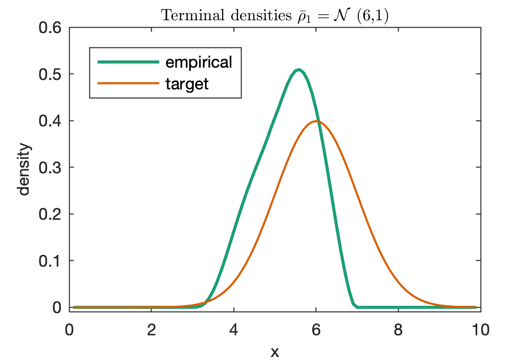
(a) $\lambda=1$

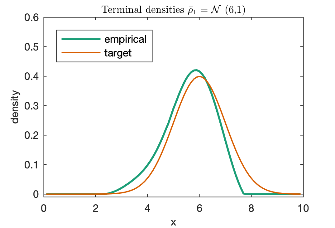
(b) $\lambda=20$

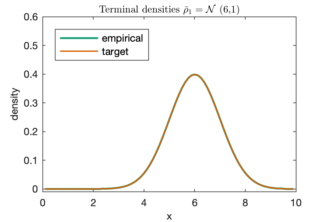
(c) infinite penalty

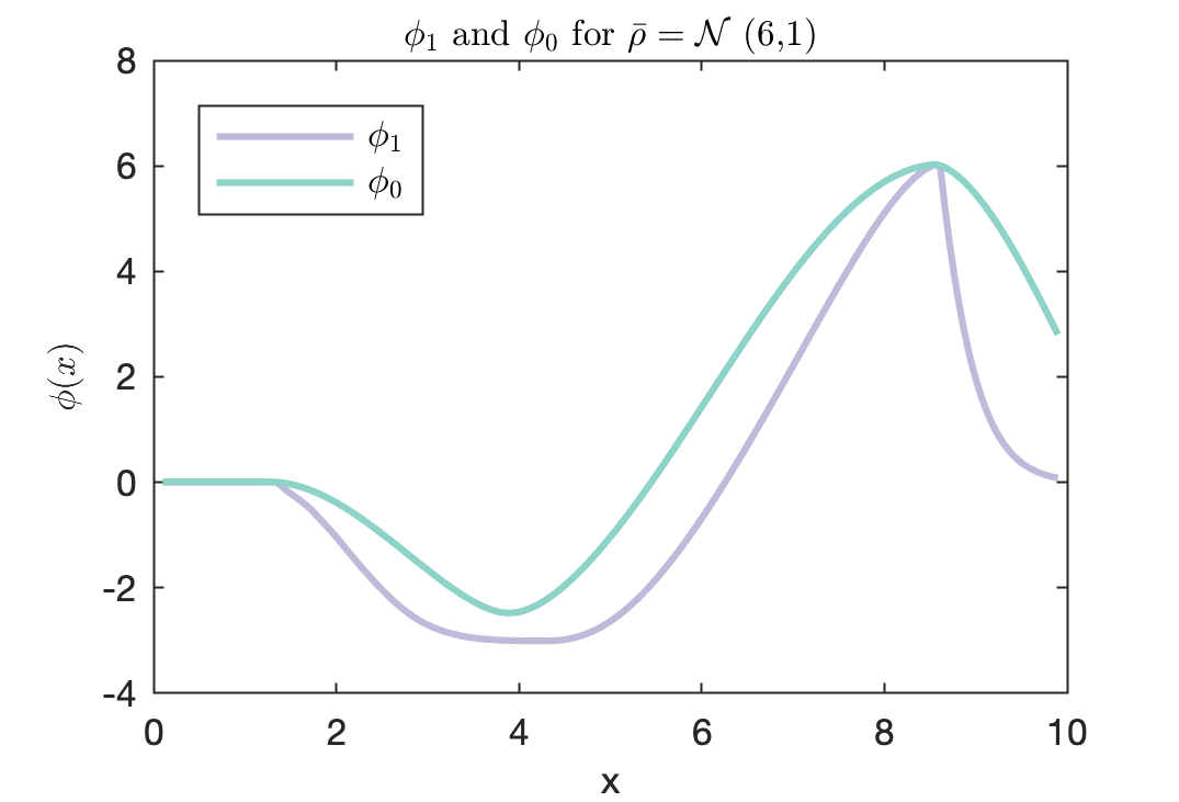
(d) optimal $\phi_{1}$ and $\phi_{0}$

Figure 1: Attainable example: $\bar{\rho}_{1}=\mathcal{N}(6,1)$

Compared to other research where the prescribed distributions are restricted to Gaussian, our method applies to a wide choice of $\bar{\rho}_{1}$, such as heavy-tailed and asymmetric distributions. In Figure 5.1, we illustrate an example where $\bar{\rho}_{1}$ is a mixture of two Normal distributions, where

$$\bar{\rho}_{1}(x)=0.5\mathcal{N}(4,1)+0.5\mathcal{N}(7,1).$$

In Figure 5.1, we plot how the Euclidean distance $\left(\int_{\mathbb{R}}(\rho_{1}-\bar{\rho}_{1})^{2}dx\right)^{\frac{1}{2}}$ changes with respect to $\lambda$ . As we increase the intensity parameter $\lambda$, the Euclidean distance between $\rho_{1}$ and $\bar{\rho}_{1}$ decreases. As $\lambda$ goes to infinity, the distance asymptotically goes to zero.

figuremixture of Normal distributions

figureDistance metric vs. $\lambda$

The Kullback–Leibler (K–L) divergence introduced in Kullback and Leibler (1951), is also known as relative entropy or information deviation. It measures the divergence of the distribution $\rho_{1}$ from the target $\bar{\rho}_{1}$, the more similar the two distributions are, the smaller the relative entropy will be. This measurement is widely used in Machine Learning to compare two densities because it has the following advantages: $1)$ this function is non-negative; $2)$ for a fixed distribution $\bar{\rho}_{1}$, $C(\rho_{1},\bar{\rho}_{1})$ is convex in $\rho_{1}$; $3)$ $C(\rho_{1},\bar{\rho}_{1})=0$ if and only if $\rho_{1}=\bar{\rho}_{1}$ everywhere. There are also caveats to the implementation of this penalty function. We may face $0\log 0$ or division by zero cases in practice; to address this, we can replace zero with an infinitesimal positive value.

In this case, the penalty functional is defined as

$$C(\rho_{1},\bar{\rho}_{1})=\int_{\mathbb{R}}\lambda\rho_{1}(x)\ln\left(\frac{\rho_{1}(x)}{\bar{\rho}_{1}(x)}\right)dx,$$ (42)

and the dual problem (26) can be expressed explicitly as

$$V(\rho_{0},\bar{\rho}_{1})=\sup_{\phi_{1}}\left\{-\int_{\mathbb{R}}\lambda\exp\left(-\frac{\phi_{1}}{\lambda}-1\right)\bar{\rho}_{1}-\phi_{0}\rho_{0}dx\right\}.$$

In Figure 2, we compare the empirical terminal density $\rho_{1}$ and the target $\bar{\rho}_{1}$ when $C(\rho_{1},\bar{\rho}_{1})$ is defined by (42) and $F(\tilde{A},\tilde{B})=(\tilde{A}-0.2)^{2}+(\tilde{B}-0.2)^{2}$. The initial wealth $x_{0}=5$ and we set $\lambda=0.1$ in Figure 2a and $\lambda=10$ in Figure 2b.

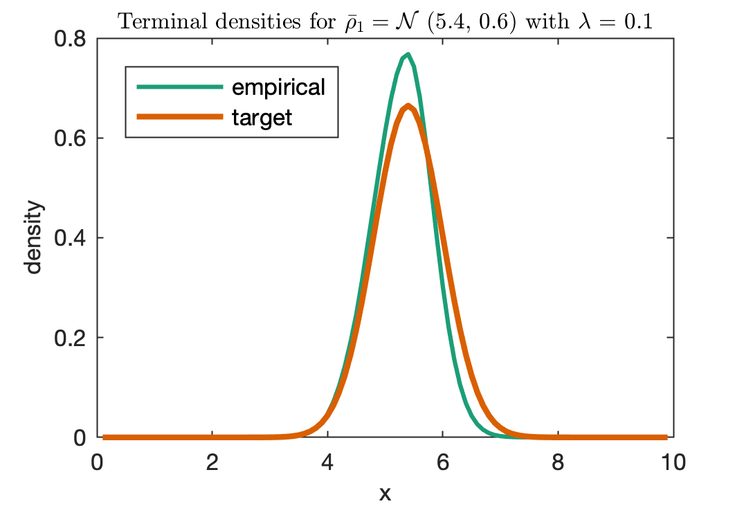
(a) $\bar{\rho}_{1}=\mathcal{N}(5.4,0.6),\lambda=0.1$

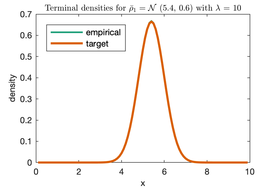
(b) $\bar{\rho}_{1}=\mathcal{N}(5.4,0.6),\lambda=10$

Figure 2: K–L divergence as the penalty functional

5.2 Distribution of the wealth with cash saving

In this section, we consider the cash saving during the investment process. From previous parts, we have the constraint $(\tilde{B}^{+})^{2}\leq\left\|\nu_{t}\right\|^{2}\tilde{A}$. However, when the prescribed target $\bar{\rho}_{1}$ is not ambitious enough, we will find the optimal drift $\tilde{B}^{*}$ is not saturated, i.e., $({\tilde{B}}^{*+})^{2}<\left\|\nu_{t}\right\|^{2}\tilde{A}^{*}$ in (31). In this case, we can actually attain a more ambitious distribution and have an accumulated cash saving $\int_{0}^{1}\left\|\nu_{t}\right\|\sqrt{\tilde{A}^{*}}-\tilde{B}^{*}dt$ during the investment process. Our goal in this section is to show that we can reach a better terminal distribution, in the sense that the terminal wealth has a higher expected value, when we take cash saving into account.

Denote $\left(C_{t}\right)_{t\in[0,1]}$ the accumulated cash saving up to time $t$, and the evolution of $C_{t}$ is

$$dC_{t} =\left(\left\|\nu_{t}\right\|\sqrt{\tilde{A}^{*}}-\tilde{B}^{*}\right)dt,$$

$$C_{0} =0.$$

If we add up the cash saving $C_{t}$ and the portfolio wealth $X_{t}$, we can get a new process wealth with cash saving. Define $X^{c}_{t}\coloneqq X_{t}+C_{t}$, it is obvious to see that $X^{c}_{t}$ follows the dynamics

$$dX^{c}_{t} =\left\|\nu_{t}\right\|\sqrt{\tilde{A}^{*}}dt+\tilde{A}^{*^{\frac{1}{2}}}dW_{t},$$

$$X^{c}_{0} =x_{0}.$$

Denote by $p(t,x)\in\mathcal{P}$ the distribution of $X^{c}_{t}$ at time $t$, then $p(t,x)$ satisfies the following Fokker-Planck equation

$$\partial_{t}p+\partial_{x}\left(\left\|\nu_{t}\right\|\sqrt{\tilde{A}^{*}}p\right)-\frac{1}{2}\partial_{xx}\left(\tilde{A}^{*}p\right) =0,$$

$$p_{0}(x) =\delta(x-x_{0}).$$

Therefore, after solving for the optimal $\tilde{A}^{*}$, $\tilde{B}^{*}$ over time, we can find the densities of $X_{t}$ as well as $X^{c}_{t}$. We keep using the squared Euclidean distance as the penalty functional and $F(\tilde{A})=(\tilde{A}-0.2)^{2}+(\tilde{B}-0.2)^{2}$ as the cost function. Figure 3 compares the densities for $X_{1}$ (terminal wealth), $X^{c}_{1}$ (terminal wealth with cash saving) and the prescribed target density. In Figure 3a, with a rather conservative target $\bar{\rho}_{1}=\mathcal{N}(5.1,0.5)$, although $\rho_{1}$ has attained the target, the distribution for the wealth with cash saving gathers at a higher value. When we set a higher target $\bar{\rho}_{1}=\mathcal{N}(6,1)$, as in Figure 3b, we see there is no cash saved in the process since the paths for $\rho_{1}$ and $p_{1}$ overlapped.

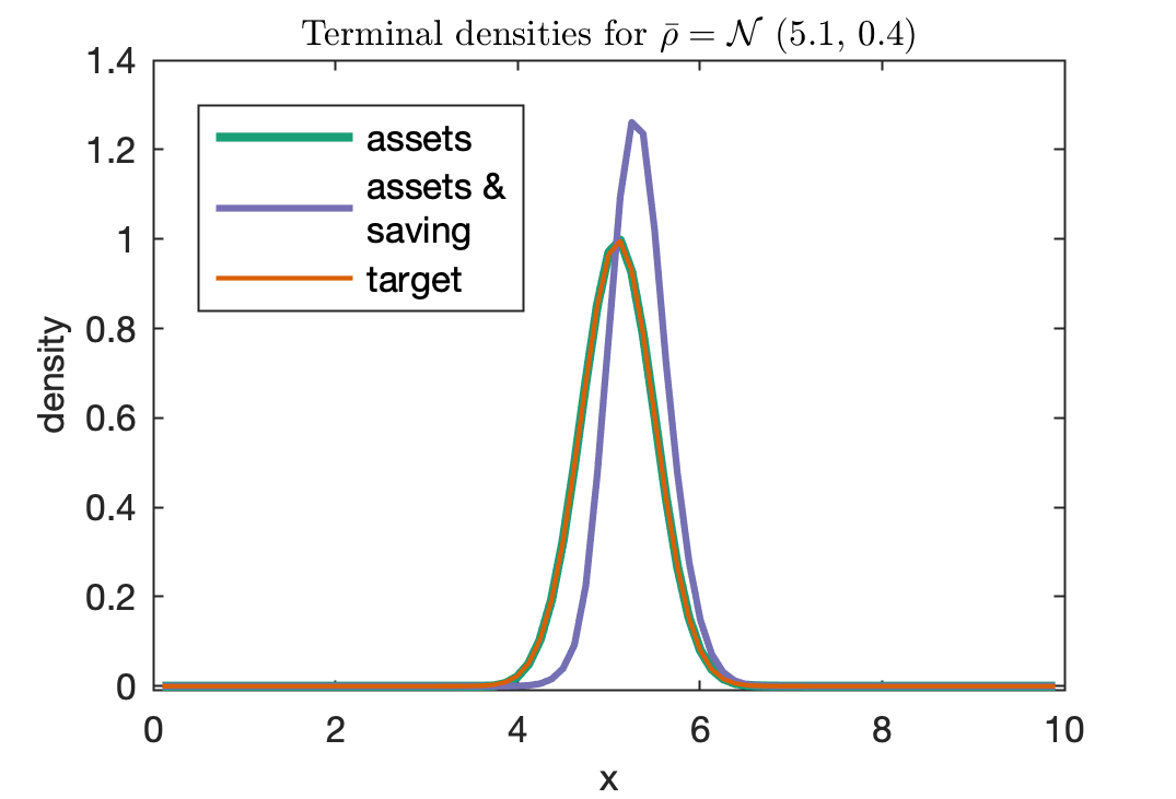
(a) $\bar{\rho}_{1}=\mathcal{N}(5.1,0.4)$

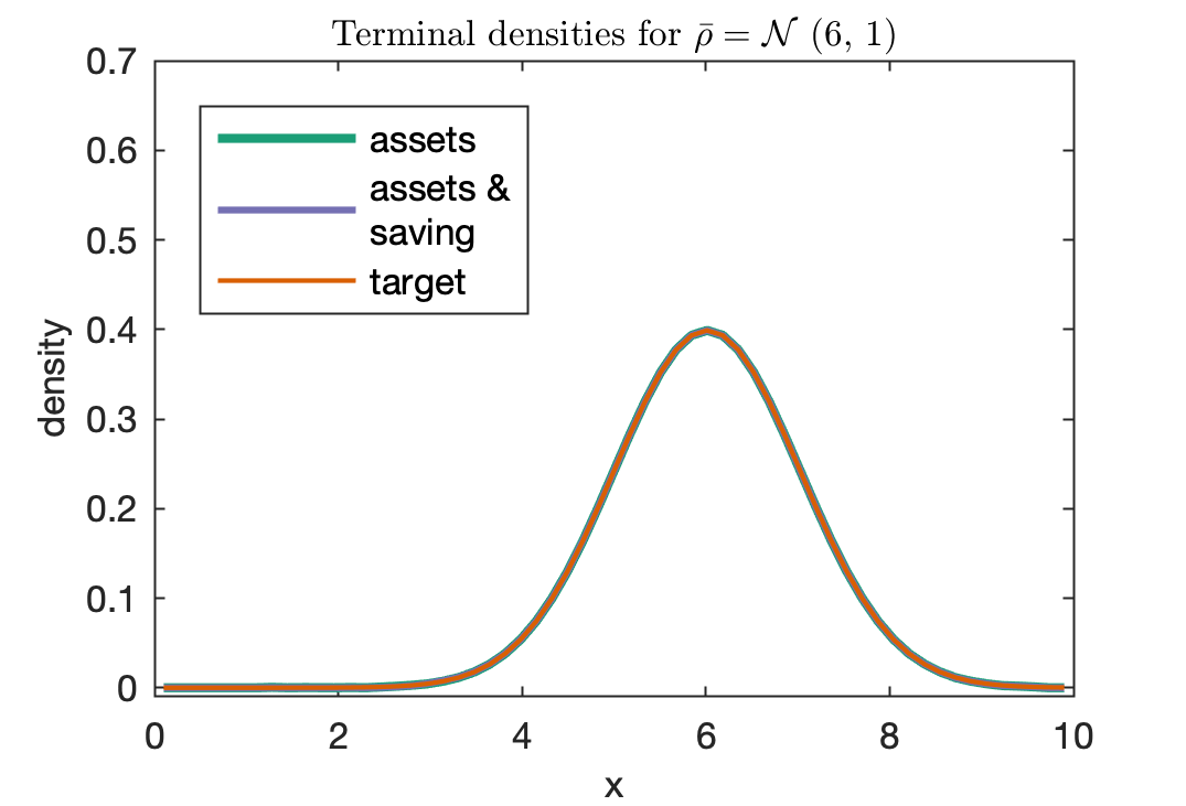
(b) $\bar{\rho}_{1}=\mathcal{N}(6,1)$

Figure 3: Compare terminal distributions with or without cash saving

5.3 Distribution of the wealth with cash input

As stated in Proposition 1, we always have $(\tilde{B}^{+})^{2}\leq\left\|\nu_{t}\right\|^{2}\tilde{A}$ for a self-financing portfolio. However, in this section, we remove the constraint $(\tilde{B}^{+})^{2}\leq\left\|\nu_{t}\right\|^{2}\tilde{A}$, and we allow $\tilde{B}\in\mathbb{R}$ instead. Then the part $\left(\tilde{B}-\left\|\nu_{t}\right\|\sqrt{\tilde{A}}\right)^{+}$ can be interpreted as the extra cash we invest during the process. In this case, theoretically, we can attain any prescribed target distribution as we want (see Tan et al. 2013, Remark 2.3). For the $\bar{\rho}_{1}$ which is unattainable by the self-financing portfolio, we can now attain it with the help of cash input. However, to limit the use of cash, we design a cost function as follows,

$$F(\tilde{A},\tilde{B})=\begin{cases}K(\tilde{B}^{2}-\left\|\nu_{t}\right\|^{2}\tilde{A})+w\tilde{A}^{2},&\quad\forall\tilde{B}>\left\|\nu_{t}\right\|\sqrt{\tilde{A}},\\ w\tilde{A}^{2},&\quad\text{$\forall$}0\leq\tilde{B}\leq\left\|\nu_{t}\right\|\sqrt{\tilde{A}},\\ l\tilde{B}^{2}+w\tilde{A}^{2},&\quad\forall\tilde{B}<0,\end{cases}$$ (43)

where $K,w,l$ are positive constants. In the cost function (43), we use the term $K(\tilde{B}^{2}-\left\|\nu_{t}\right\|^{2}\tilde{A})$ to penalize the part $\left(\tilde{B}-\left\|\nu_{t}\right\|\sqrt{\tilde{A}}\right)^{+}$. By varying $K$, we can control the strength of penalty and hence control the cash input flow. When $K$ is small, we are allowed to put in cash without being penalized excessively. When $K$ is large, we have to pay a high price for the cash input; consequently, the usage is limited. The terms $w\tilde{A}^{2}$ and $l\tilde{B}^{2}$ add coercivity to the function to ensure the existence of the solution, we set $w,l$ to be small positive real values.

With the optimal drift $\tilde{B}^{*}\in\mathbb{R}$ and diffusion $\tilde{A}^{*}\in\mathbb{R}^{+}$, the dynamics of the wealth $X_{t}$ is

$$dX_{t} =\tilde{B}^{*}dt+\sqrt{\tilde{A}^{*}}dW_{t},$$

$$X_{0} =x_{0}.$$

If there is no cash input, the maximum drift is $\left\|\nu_{t}\right\|\sqrt{\tilde{A}}$. Denote $\left(I_{t}\right)_{t\in[0,1]}$ the accumulated cash input up to time $t$, and $I_{t}$ follows the dynamics

$$dI_{t} =\left(\tilde{B}^{*}-\left\|\nu_{t}\right\|\sqrt{\tilde{A}^{*}}\right)^{+}dt,$$

$$I_{0} =0.$$

Define $X^{I}_{t}\coloneqq X_{t}-I_{t}$ as the path without the cash input. Then the dynamics of $X^{I}_{t}$ is

$$dX^{I}_{t} =\min\left(\tilde{B}^{*},\left\|\nu_{t}\right\|\sqrt{\tilde{A}^{*}}\right)dt+\sqrt{\tilde{A}^{*}}dW_{t},$$

$$X^{I}_{0} =x_{0}.$$

Let the density of $X^{I}_{t}$ be $q(t,x)\in\mathcal{P}$, then $q(t,x)$ follows the following Fokker-Planck equation

$$\partial_{t}q+\partial_{x}\left[\min\left(\tilde{B}^{*},\left\|\nu_{t}\right\|\sqrt{\tilde{A}^{*}}\right)q\right]-\frac{1}{2}\partial_{xx}\left(\tilde{A}^{*}q\right) =0,$$

$$q_{0}(x) =\delta(x-x_{0}).$$

Finally, we can see the effect of cash input by comparing $\rho_{1}(x)$ and $q_{1}(x)$.

5.3.1 Attainable target

In the first example, we aim at the terminal distribution $\bar{\rho}_{1}=\mathcal{N}(6,1)$, which is attainable by the self-financing portfolio. We use the squared Euclidean distance as the penalty functional and equation (43) as the cost function. Figure 4 demonstrates the time evolution of $q(t,x)$ (assets) and $\rho(t,x)$ (assets and cash input), and it compares $q_{1}(x),\rho_{1}(x)$ and $\bar{\rho}_{1}(x)$ for various $K$ values. At the beginning, we set the coefficient $K=0.5$ in Figure 4a. There is a clear difference between the paths for assets and assets and cash, which means we have input a significant amount of cash over time. As we increase the value of $K$ in Figure 4b, the difference between $q(t,x)$ and $\rho(t,x)$ becomes less obvious. When $K=6$, the paths with or without cash input coincide in Figure 4c because the high cost has prevented the cash input in this context. Since the target $\mathcal{N}(6,1)$ is attainable, we can still reach it even without cash input, as shown in the second plot of 4c.

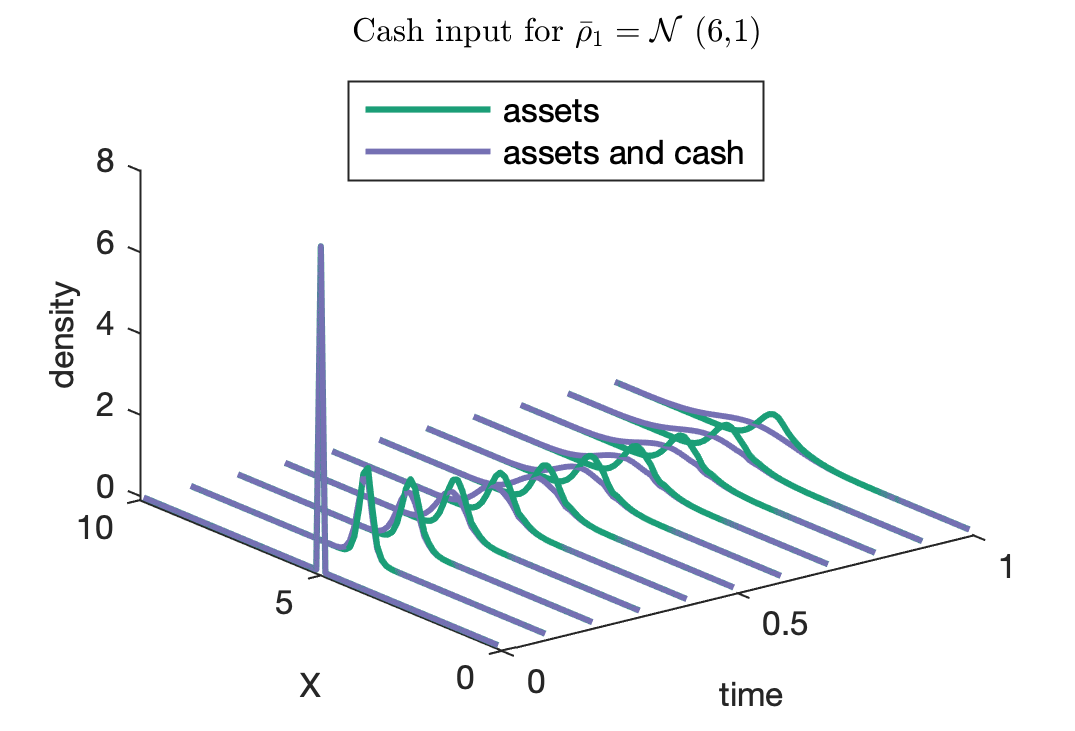
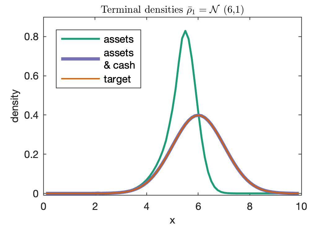
(a) $K=0.5$

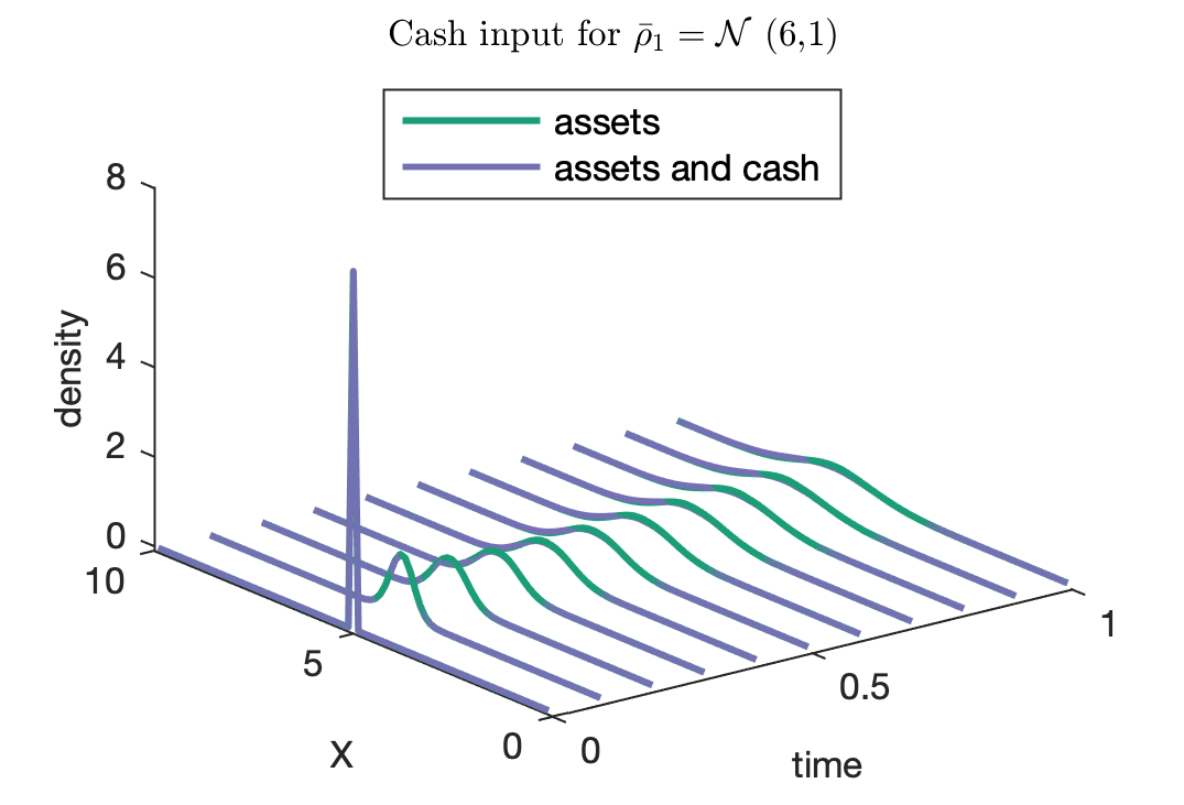
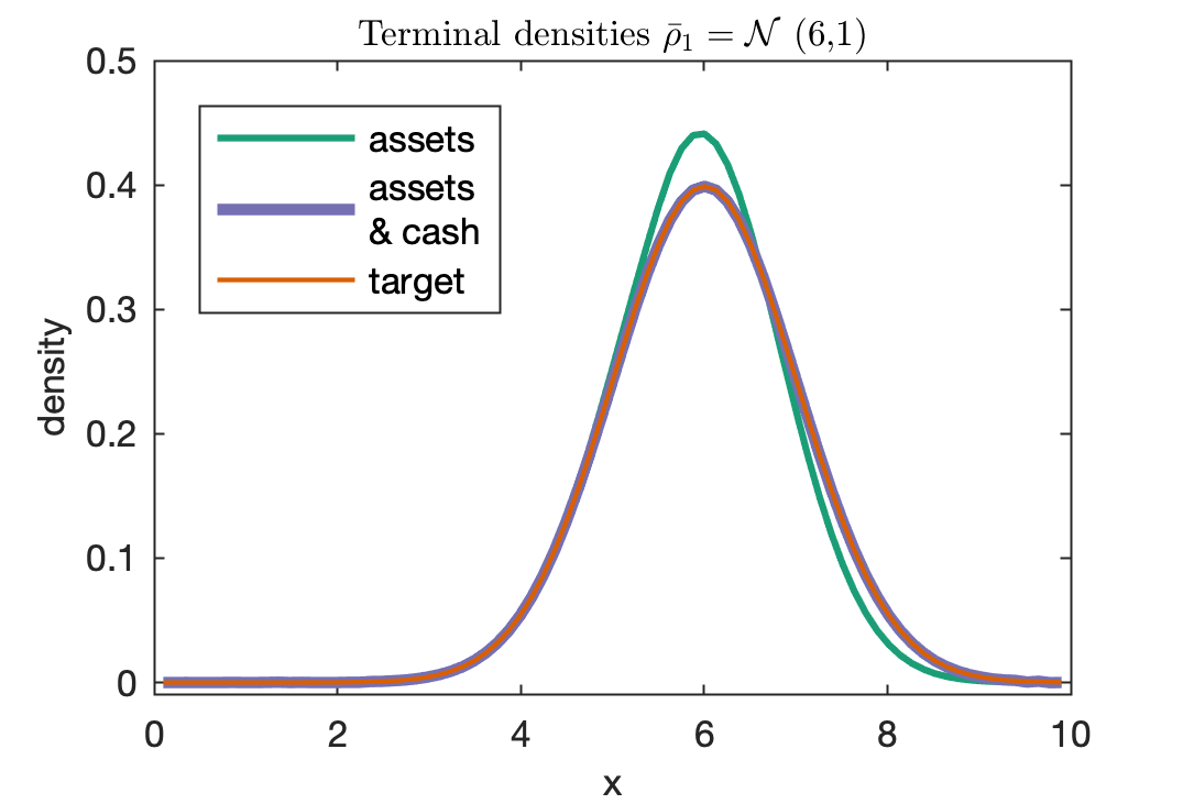
(b) $K=4$

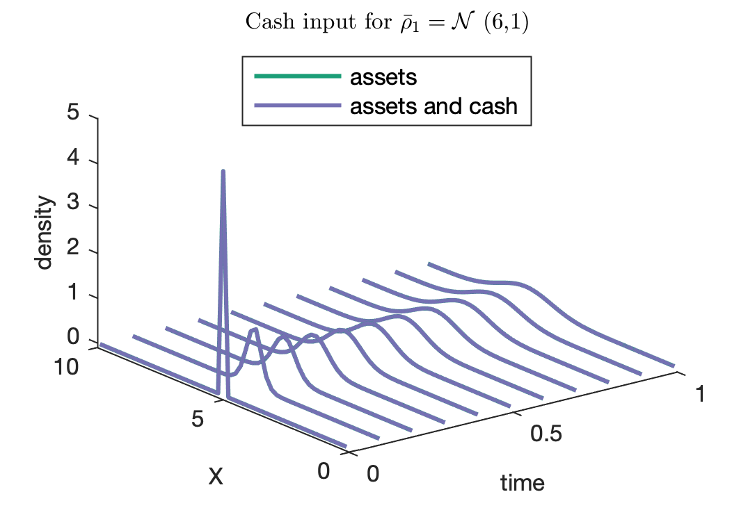
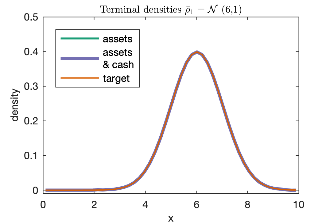
(c) $K=6$

Figure 4: Fixed $K$ for an attainable target: $\bar{\rho}_{1}=\mathcal{N}(6,1)$

5.3.2 Unattainable target

To see the effect of cash input, here we demonstrate an example with an unattainable target. For instance, we may target at a terminal distribution with no left tail but a heavy right tail, in other words, there is very little risk for the wealth to fall below some level. Therefore, we set $\bar{\rho}_{1}=Weibull\,(6,2)$ in Figure 5a, where $P(x<4)$ is almost zero. In this example, the coefficient $K$ in (43) is not a constant anymore. Instead, we let $K(t):[0,1]\rightarrow\mathbb{R}^{+}$ be a function of time so that we can control the cash input flow over time. We define $K(t)=5$ for $t\in[0,0.8]$ and $K(t)=0.1$ for $t\in[0.8,1]$. In the time-evolution plot (the left one of Figure 5a), we can see that the paths for assets and assets and cash start to differentiate from $t=0.8$. Similarly, we can see the same effect in Figure 5b, where we set $\bar{\rho}_{1}=\mathcal{N}(6.5,1)$ and we define $K(t)=5$ for $t\in[0,0.95]$ and $K(t)=0.1$ for $t\in[0.95,1]$. In these two examples, the targets $Weibull\,(6,2)$ and $\mathcal{N}(6.5,1)$ are unattainable under the constraint $(\tilde{B}^{+})^{2}\leq\left\|\nu_{t}\right\|^{2}\tilde{A}$. However, we can make the empirical terminal density $\rho_{1}$ reach $\bar{\rho}_{1}$ by inputting cash wisely.

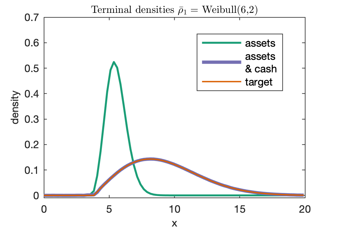
(a) $K=5\>\forall t\in[0,0.8],K=0.1\>\forall t\in[0.8,1]$ for Weibull $(6,2)$

(b) $K=5\>\forall t\in[0,0.95],K=0.1\>\forall t\in[0.95,1]$ for $\mathcal{N}(6.5,1)$

Figure 5: $K(t)$ for unattainable targets

6 Conclusion

The ability to specify the whole distribution of final wealth of interest as portfolio optimization target gives a greater flexibility over classical objective functions such as expected utility or moment-based objectives such as the mean-variance framework and its extensions. In this article, we construct a portfolio and the dynamics of the portfolio wealth is a semimartingale. Starting from an initial wealth, by controlling the portfolio allocation process, we are able to steer the portfolio wealth to a prescribed distribution at the terminal time. This problem is closely related to optimal mass transport (OMT). In the problem formulation, in addition to the conventional cost function in OMT, we also design a penalty functional to measure the divergence of the empirical terminal density from the prescribed one. We take into consideration the possible consumption during the investment process, and show that we can actually reach a better terminal density when there is no consumption. When the target density is attainable, our problem can recover the classical OMT problem by choosing an indicator function as the penalty function. When the target terminal density is unattainable by the self-financing portfolio, we devise a strategy to reach it by allowing cash input during the investment process. We proved a duality result for the primal problem and solved it with a gradient descent based algorithm. Our numerical results verify the accuracy and validity of this algorithm.

Appendix A Appendices

A.1

Proof of Proposition 1.

 

Firstly, we prove the necessity. We can use eigen-decomposition and write the covariance matrix $\Sigma_{t}=Q\Lambda Q^{{}^{\intercal}}=Q\Lambda^{\frac{1}{2}}\Lambda^{\frac{1}{2}}Q^{\intercal}$, where $Q\in\mathbb{R}^{d\times d}$ and the $i$th column of $Q$ is the eigenvector $q_{i}$ of $\Sigma_{t}$, and $\Lambda\in\mathbb{R}^{d\times d}$ is the diagonal matrix whose diagonal elements are the corresponding eigenvalues, $\Lambda_{ii}=\lambda_{i}$.

For any given $\alpha_{t}\in\mathbb{R}^{d}$, $A=\alpha_{t}^{\intercal}Q\Lambda^{\frac{1}{2}}\Lambda^{\frac{1}{2}}Q^{\intercal}\alpha_{t}x^{2}\rho$. We define $\beta\coloneqq\alpha_{t}^{\intercal}Q\Lambda^{\frac{1}{2}}$, then $A=\beta\beta^{\intercal}x^{2}\rho=\left\|\beta\right\|^{2}x^{2}\rho$, where $\left\|\cdot\right\|$ denotes the $L^{2}$ norm. Similarly, $B=\alpha_{t}^{\intercal}Q\Lambda^{\frac{1}{2}}(Q\Lambda^{\frac{1}{2}})^{-1}\mu_{t}x\rho=\beta(Q\Lambda^{\frac{1}{2}})^{-1}\mu_{t}x\rho$. Therefore we have the relationship between $A$ and $B$ as

$$B^{2}=\left(\beta(Q\Lambda^{\frac{1}{2}})^{-1}\mu_{t}\right)^{2}x^{2}\rho^{2}\leq\left\|\beta\right\|^{2}\left\|(Q\Lambda^{\frac{1}{2}})^{-1}\mu_{t}\right\|^{2}x^{2}\rho^{2}=A\rho\left\|(Q\Lambda^{\frac{1}{2}})^{-1}\mu_{t}\right\|^{2},$$

$$\left\|(Q\Lambda^{\frac{1}{2}})^{-1}\mu_{t}\right\|^{2}A\geq\frac{B^{2}}{\rho}.$$

Define $\nu_{t}\coloneqq(Q\Lambda^{\frac{1}{2}})^{-1}\mu_{t}=\Sigma_{t}^{-\frac{1}{2}}\mu_{t}$, we can write the above inequality as $A\geq\frac{B^{2}}{\left\|\nu_{t}\right\|^{2}\rho}$.

For given $(\rho,B,A)$ satisfying $A\geq\frac{B^{2}}{\left\|\nu_{t}\right\|^{2}\rho}$, we want to show that there exists $\alpha_{t}\in\mathbb{R}^{d}(d>1)$, such that $A=\alpha_{t}^{\intercal}\Sigma_{t}\alpha_{t}x^{2}\rho$, $B=\alpha_{t}^{\intercal}\mu_{t}x\rho$. First of all, since $\frac{A}{\rho}\geq 0$, there exists a vector $\beta\in\mathbb{R}^{1\times d}$ whose norm satisfies $\left\|\beta\right\|^{2}=\frac{A}{x^{2}\rho}$. Then $\frac{B^{2}}{\left\|\nu_{t}\right\|^{2}\rho}\leq A$ will be equivalent to $B^{2}\leq\left\|\beta\right\|^{2}\left\|\nu_{t}\right\|^{2}x^{2}\rho^{2}$. With Cauchy–Schwarz inequality, $(\beta\nu_{t})^{2}x^{2}\rho^{2}\leq\left\|\beta\right\|^{2}\left\|\nu_{t}\right\|^{2}x^{2}\rho^{2}$ holds. Therefore there exists a vector $\beta\in\mathbb{R}^{1\times d}(d>1)$ such that $B=\beta\nu_{t}x\rho$ and $\left\|\beta\right\|^{2}=\frac{A}{x^{2}\rho}$. With this $\beta$, there exists an $\alpha_{t}=Q\Lambda^{-\frac{1}{2}}\beta^{\intercal}$.

The case for dimension $d=1$ is trivial, hence omitted here. ∎

A.2

Proposition 2.

We denote $K_{0}$ the set of $(u,b,a,r)\in C_{b}(\mathcal{E},\mathbb{R}\times\mathbb{R}\times\mathbb{R}\times\mathbb{R})$ that can be represented by $\phi\in C_{b}^{1,2}(\mathcal{E})$. Then we have

$$\inf_{(\rho,B,A,\rho_{1})\in C_{b}^{*}(\mathcal{E};\mathbb{R}\times\mathbb{R}\times\mathbb{R}\times\mathbb{R})}\left\{\alpha^{*}(\rho,B,A,\rho_{1})+\beta^{*}(\rho,B,A,\rho_{1})\right\}=\inf_{(\rho,B,A,\rho_{1})\in\mathcal{M}(\mathcal{E};\mathbb{R}\times\mathbb{R}\times\mathbb{R}\times\mathbb{R})}\left\{\alpha^{*}(\rho,B,A,\rho_{1})+\beta^{*}(\rho,B,A,\rho_{1})\right\}.$$

Proof.

Following closely the argument in Villani (2003, Section 1.3), we define $C_{0}(\mathcal{E})$ the space of continuous functions on $\mathcal{E}$, going to $0$ at infinity. For $(\rho,B,A,\rho_{1})\in C_{b}^{*}(\mathcal{E};\mathbb{R}\times\mathbb{R}\times\mathbb{R}\times\mathbb{R})$, we decompose $(\rho,B,A,\rho_{1})=(\hat{\rho},\hat{B},\hat{A},\hat{\rho}_{1})+(\delta\rho,\delta B,\delta A,\delta\rho_{1})$, where $(\hat{\rho},\hat{B},\hat{A},\hat{\rho}_{1})\in\mathcal{M}(\mathcal{E};\mathbb{R}\times\mathbb{R}\times\mathbb{R}\times\mathbb{R})$. For any $(u,b,a,r)\in C_{0}(\mathcal{E};\mathbb{R}\times\mathbb{R}\times\mathbb{R}\times\mathbb{R})$, we have $\langle(u,b,a,r),(\delta\rho,\delta B,\delta A,\delta\rho_{1})\rangle=0$.

Because $\mathcal{M}(\mathcal{E};\mathbb{R})$ is a subset of $C_{b}^{*}(\mathcal{E};\mathbb{R})$, we naturally have

$$\inf_{(\rho,B,A,\rho_{1})\in C_{b}^{*}(\mathcal{E};\mathbb{R}\times\mathbb{R}\times\mathbb{R}\times\mathbb{R})}\left\{\alpha^{*}(\rho,B,A,\rho_{1})+\beta^{*}(\rho,B,A,\rho_{1})\right\}\leq\inf_{(\rho,B,A,\rho_{1})\in\mathcal{M}(\mathcal{E};\mathbb{R}\times\mathbb{R}\times\mathbb{R}\times\mathbb{R})}\left\{\alpha^{*}(\rho,B,A,\rho_{1})+\beta^{*}(\rho,B,A,\rho_{1})\right\}.$$ (44)

Now we look at the opposite direction of inequality (44). For $\alpha^{*}$, we have

$$\alpha^{*}(\rho,B,A,\rho_{1}) =\sup_{(u,b,a,r)\in C_{b}(\mathcal{E};\mathbb{R}\times\mathbb{R}\times\mathbb{R}\times\mathbb{R})}\Bigl{\{}\int_{\mathcal{E}}ud\rho+bdB+adA+\Bigl{[}\int_{\mathbb{R}}rd\rho_{1}-C^{*}(r)\Bigr{]}:u+F^{*}(b,a)\leq 0\Bigr{\}}$$

$$\geq\sup_{(u,b,a,r)\in C_{0}(\mathcal{E};\mathbb{R}\times\mathbb{R}\times\mathbb{R}\times\mathbb{R})}\Bigl{\{}\int_{\mathcal{E}}ud\rho+bdB+adA+\Bigl{[}\int_{\mathbb{R}}rd\rho_{1}-C^{*}(r)\Bigr{]}:u+F^{*}(b,a)\leq 0\Bigr{\}}$$

$$=\sup_{(u,b,a,r)\in C_{0}(\mathcal{E};\mathbb{R}\times\mathbb{R}\times\mathbb{R}\times\mathbb{R})}\Bigl{\{}\int_{\mathcal{E}}ud\hat{\rho}+bd\hat{B}+ad\hat{A}+\Bigl{[}\int_{\mathbb{R}}rd\hat{\rho}_{1}-C^{*}(r)\Bigr{]}:u+F^{*}(b,a)\leq 0\Bigr{\}}$$

$$=\alpha^{*}(\hat{\rho},\hat{B},\hat{A},\hat{\rho}_{1}).$$

We know $\beta^{*}(\hat{\rho},\hat{B},\hat{A},\hat{\rho}_{1})=0$ if $(\hat{\rho},\hat{B},\hat{A},\hat{\rho}_{1})$ satisfies (21), and $\beta^{*}(\hat{\rho},\hat{B},\hat{A},\hat{\rho}_{1})=+\infty$ otherwise. When $\beta^{*}$ is finite,

$$\int_{\mathcal{E}}ud\hat{\rho}+bd\hat{B}+ad\hat{A}+\int_{\mathbb{R}}rd\hat{\rho}_{1}-\phi_{0}d\rho_{0}=0\qquad\forall(u,b,a,r)\in K_{0}.$$

Then we have

$$\beta^{*}(\hat{\rho},\hat{B},\hat{A},\hat{\rho}_{1}) =\sup_{(u,b,a,r)\in C_{0}\cap K_{0}}\int_{\mathcal{E}}ud\hat{\rho}+bd\hat{B}+ad\hat{A}+\int_{\mathbb{R}}rd\hat{\rho}_{1}-\phi_{0}d\rho_{0}$$

$$=\sup_{(u,b,a,r)\in C_{0}\cap K_{0}}\int_{\mathcal{E}}ud\rho+bdB+adA+\int_{\mathbb{R}}rd\rho_{1}-\phi_{0}d\rho_{0}$$

$$\leq\sup_{(u,b,a,r)\in K_{0}}\int_{\mathcal{E}}ud\rho+bdB+adA+\int_{\mathbb{R}}rd\bar{\rho}_{1}-\phi_{0}d\rho_{0}$$

$$=\beta^{*}(\rho,B,A,\rho_{1}).$$

This completes the proof. ∎

References

- Benamou and Brenier (2000) Benamou, J.-D. and Y. Brenier (2000). A computational fluid mechanics solution to the Monge-Kantorovich mass transfer problem. Numerische Mathematik 84(3), 375–393.
- Benamou et al. (2019) Benamou, J.-D., G. Carlier, and L. Nenna (2019). Generalized incompressible flows, multi-marginal transport and Sinkhorn algorithm. Numerische Mathematik 142(1), 33–54.
- Brenier et al. (2003) Brenier, Y., U. Frisch, M. Henon, G. Loeper, S. Matarrese, R. Mohayaee, and A. Sobolevskii (2003). Reconstruction of the early universe as a convex optimization problem. arxiv (september 2003). arXiv preprint astro-ph/0304214.
- Brezis (2010) Brezis, H. (2010). Functional analysis, Sobolev spaces and partial differential equations. Springer Science & Business Media.
- Cha (2007) Cha, S.-H. (2007). Comprehensive survey on distance/similarity measures between probability density functions. City 1(2), 1.
- Chartrand et al. (2009) Chartrand, R., B. Wohlberg, K. Vixie, and E. Bollt (2009). A gradient descent solution to the Monge-Kantorovich problem. Applied Mathematical Sciences 3(22), 1071–1080.
- Cuturi (2013) Cuturi, M. (2013). Sinkhorn distances: Lightspeed computation of optimal transport. In Advances in neural information processing systems, pp. 2292–2300.
- Dolinsky and Soner (2014) Dolinsky, Y. and H. M. Soner (2014). Martingale optimal transport and robust hedging in continuous time. Probability Theory and Related Fields 160(1-2), 391–427.
- Ferradans et al. (2014) Ferradans, S., N. Papadakis, G. Peyré, and J.-F. Aujol (2014). Regularized discrete optimal transport. SIAM Journal on Imaging Sciences 7(3), 1853–1882.
- Guo et al. (2019) Guo, I., N. Langrené, G. Loeper, and W. Ning (2019). Robust utility maximization under model uncertainty via a penalization approach. arXiv preprint arXiv:1907.13345.
- Guo et al. (2019) Guo, I., G. Loeper, and S. Wang (2019). Calibration of local-stochastic volatility models by optimal transport. arXiv preprint arXiv:1906.06478.
- Henry-Labordère (2017) Henry-Labordère, P. (2017). Model-free hedging: A martingale optimal transport viewpoint. CRC Press.
- Henry-Labordère et al. (2016) Henry-Labordère, P., X. Tan, and N. Touzi (2016). An explicit martingale version of the one-dimensional Brenier’s theorem with full marginals constraint. Stochastic Processes and their Applications 126(9), 2800–2834.
- Kantorovich (1942) Kantorovich, L. V. (1942). On the translocation of masses. In Dokl. Akad. Nauk. USSR (NS), Volume 37, pp. 199–201.
- Kraus and Litzenberger (1976) Kraus, A. and R. H. Litzenberger (1976). Skewness preference and the valuation of risk assets. The Journal of finance 31(4), 1085–1100.
- Kullback and Leibler (1951) Kullback, S. and R. A. Leibler (1951). On information and sufficiency. The annals of mathematical statistics 22(1), 79–86.
- Lee (1977) Lee, C. F. (1977). Functional form, skewness effect, and the risk-return relationship. Journal of financial and quantitative analysis 12(1), 55–72.
- Loeper (2006) Loeper, G. (2006). The reconstruction problem for the Euler-Poisson system in cosmology. Archive for rational mechanics and analysis 179(2), 153–216.
- Markowitz (1952) Markowitz, H. (1952). Portfolio selection. The journal of finance 7(1), 77–91.
- Mikami (2015) Mikami, T. (2015). Two end points marginal problem by stochastic optimal transportation. SIAM Journal on Control and Optimization 53(4), 2449–2461.
- Mikami and Thieullen (2006) Mikami, T. and M. Thieullen (2006). Duality theorem for the stochastic optimal control problem. Stochastic processes and their applications 116(12), 1815–1835.
- Monge (1781) Monge, G. (1781). Mémoire sur la théorie des déblais et des remblais. Histoire de l’Académie Royale des Sciences de Paris.
- Rachev and Rüschendorf (1998) Rachev, S. T. and L. Rüschendorf (1998). Mass Transportation Problems: Volume I: Theory, Volume 1. Springer Science & Business Media.
- Tan et al. (2013) Tan, X., N. Touzi, et al. (2013). Optimal transportation under controlled stochastic dynamics. The annals of probability 41(5), 3201–3240.
- Villani (2003) Villani, C. (2003). Topics in optimal transportation. Number 58. American Mathematical Soc.
- Villani (2008) Villani, C. (2008). Optimal transport: old and new, Volume 338. Springer Science & Business Media.