Effective-one-body waveforms from dynamical captures in black hole binaries

Abstract

Dynamical capture is a possible formation channel for BBH mergers leading to highly eccentric merger dynamics and to gravitational wave (GW) signals that are morphologically different from those of quasi-circular mergers. The future detection of these mergers by ground-based or space-based GW interferometers can provide invaluable insights on astrophysical black holes, but it requires precise predictions and dedicated waveform models for the analysis. We present a state-of-the-art effective-one-body (EOB) model for the multipolar merger-ringdown waveform from dynamical capture black-hole mergers with arbitrary mass-ratio and nonprecessing spins. The model relies on analytical descriptions of the radiation reaction and waveform along generic orbits that are obtained by incorporating generic Newtonian prefactors in the expressions used in the quasi-circular case. It provides a tool for generating waveforms for generic binary black hole coalescences and for GW data analysis. We demonstrate that the model reliably accounts for the rich phenomenology of dynamical captures, from direct plunge to successive close encounters up to merger. The parameter space is fully characterized in terms of the initial energy and angular momentum. Our model reproduces to few percent the scattering angle from ten equal-mass, nonspinning, hyperbolic encounter numerical-relativity (NR) simulations. The agreement can be further improved to the by incorporating 6PN-results in one of the EOB potentials and tuning currently unknown analytical parameters. Our results suggest that NR simulations of hyperbolic encounters (and dynamical captures) can be used to inform EOB waveform models for generic BBH mergers/encounters for present and future GW detectors.

I Introduction

In dense stellar regions, e.g. galactic nuclei or globular clusters, individual black holes can become gravitationally bound as energy is lost to gravitational radiation during a close passage Rasskazov and Kocsis (2019); Tagawa et al. (2020). Such dynamically captured pairs may be sources of gravitational radiation, with a phenomenology that is radically different from quasi-circular inspirals Zevin et al. (2019); Samsing and D’Orazio (2018) and can be detected from larger distances and mass than quasi-circular mergers O’Leary et al. (2009). Although to date there is no observational evidence of these systems, the capture of a stellar-mass object by a massive black hole is also expected to be an efficient emitter of gravitational radiation for future detectors as the Einstein Telescope and LISA Amaro-Seoane (2018).

Due to the special waveform morphology, these systems might be either missed or incorrectly analyzed using standard quasi-circular templates, as already emphasized long ago East et al. (2013) (see Ref. Loutrel (2020) for a recent review). Physically faithful waveform models to systematically study the phenomenology of dynamical capture do not currently exists. To our knowledge, the only attempt at building a waveform model for these kind of events dates back to Ref. East et al. (2013) that provided a qualitative study of the phenomenon. The model of East et al. (2013) is based on geodesic motion on a Kerr black hole spacetime augmented by leading-order Newtonian-like radiation reaction, then complemented by an effective model for a (quasi-circular) ringdown informed by NR simulations. Similarly, numerical relativity (NR) studies of BBH mergers from dynamical capture conducted thus far are only few Gold and Brügmann (2013); Nelson et al. (2019); Bae et al. (2020) and limited to nonspinning binaries.

Reference Damour et al. (2014) shows that the effective one body (EOB) approach to the general relativistic two-body dynamics Buonanno and Damour (1999, 2000); Damour et al. (2000); Damour (2001); Damour et al. (2008); Nagar (2011); Damour et al. (2015) is suitable also for hyperbolic scattering events. In particular, Ref. Damour et al. (2014) compares NR and EOB predictions for the scattering angles for hyperbolic encounters, although it provides neither a description for the dynamical capture, nor a waveform model. The aim of this paper is to go beyond the results of Ref. Damour et al. (2014) and illustrate that the EOB formalism can provide a complete model, for both dynamics and radiation, for dynamical capture black hole binaries. This model, which is publicly available as a stand-alone $C$ implementation teo , once optimized further, could be used for data analysis purposes, hopefully filling an evident gap in currently available waveform models. The key analytical advance used in this work is the radiation reaction and waveform along generic orbits proposed in Ref. Chiaramello and Nagar (2020). The latter is based on the use of generic (noncircular) Newtonian prefactors in the (multipolar) waveform and radiation reaction. The merger and ringdown parts of the waveform are then modeled using analytical representations informed by quasi-circular (spin-aligned) numerical simulations Nagar et al. (2017, 2019, 2020). The approach developed here represents the state-of-art within the currently available analytical knowledge. However, it is currently impossible to make precise quantitative statements on the actual faithfulness of the analytical waveforms because of the lack of systematic predictions from NR simulations of dynamical capture coalescing binaries. Moreover, the existing NR results, e.g. East et al. (2013); Gold and Brügmann (2013); Nelson et al. (2019) are not expressed using gauge-invariant observables and so it is impossible to extract any kind of information that could be directly compared with our model. Instead, we will provide an up-to-date comparison with the measured scattering angle of Ref. Damour et al. (2014).

The paper is organized as follows. In Sec. II we briefly review the eccentric EOB model of Ref. Chiaramello and Nagar (2020), focusing in particular on the initial data setup, as proposed already in Ref. Damour et al. (2014). Section III gives an overview of the possible waveform phenomenology, considering both nonspinning and spinning cases as well as higher multipolar modes. In Sec. IV we build upon Ref. Damour et al. (2014), providing a new comparison between EOB and NR scattering angles, with special emphasis on the impact of recently computed 5PN and 6PN results Bini et al. (2019, 2020a, 2020b, 2020c). In addition, differently from Ref. Damour et al. (2014) that was also relying on NR-computed fluxes, the computation of the scattering angle presented here is fully self-consistent within the EOB formalism. Finally, in Sec. V we briefly summarize our findings and set the stage for future work. Geometric units with $G=c=1$ are employed unless otherwise specified.

II EOB waveform model for dynamical captures

II.1 Overview

Reference Chiaramello and Nagar (2020) introduced an EOB model valid along generic orbits, i.e. valid for any configuration beyond the quasi-circular one. Although the analysis of Ref. Chiaramello and Nagar (2020) was limited to configurations with mild eccentricities (${\rm e}\simeq 0.3$) there are no conceptual constraints that prevent one from using the model in more extreme configurations, e.g. scattering and/or dynamical captures. The eccentric EOB model we shall use here stems from the quasi-circular one TEOBiResumS_SM Nagar et al. (2019, 2020), i.e. the most developed version of TEOBResumS Nagar et al. (2018) that incorporates subdominant waveform modes up to $\ell=m=5$. To generalize TEOBiResumS_SM to generic orbits, Ref. Chiaramello and Nagar (2020) proposed to simply replace the quasi-circular leading order terms, both in radiation reaction and waveform, with their exact analytical expressions valid on general orbits. The waveform is then completed using a model of (multipolar) merger and ringdown informed by quasi-circular NR simulations Damour and Nagar (2014a); Nagar et al. (2020). For all technical details we refer the reader to Refs. Chiaramello and Nagar (2020); Nagar et al. (2020). We just recall the notation that will be useful in the reminder of the paper. The two objects have masses $(m_{1},m_{2})$, with the convention that $m_{1}\geq m_{2}$ and the mass ratio is defined as $q\equiv m_{1}/m_{2}\geq 1$. The total mass is $M=m_{1}+m_{2}$, the reduced mass $\mu\equiv m_{1}m_{2}/M$ and the symmetric mass ratio $\nu\equiv\mu/M$. We use phase-space dimensionless variables $(r,p_{r_{*}},\varphi,p_{\varphi})$, related to the physical ones $(R,P_{r_{*}},\varphi,P_{\varphi})$ by $r=R/GM$ (relative separation), $p_{r_{*}}=P_{R_{*}}/\mu$ (radial momentum), $p_{\varphi}=P_{\varphi}/(\mu GM)$ (angular momentum), and $t\equiv T/(GM)$ the dimensionless time. The radial momentum $p_{r_{*}}$ is defined as $p_{r_{*}}=(A/B)^{1/2}\ p_{r}$, where $A$ and $B$ are the EOB metric potentials (see below). The EOB (reduced) Hamiltonian describing the relative dynamics reads

$$\hat{H}_{\rm EOB}\equiv H_{\rm EOB}\mu^{-1}=\nu^{-1}\sqrt{1+2\nu(\hat{H}_{\rm eff}-1)},$$ (1)

while the effective Hamiltonian $\hat{H}_{\rm eff}$ is split in a spin-orbit part (i.e. odd in spins) and in the orbital part (i.e. even in spin)

$$\hat{H}_{\rm eff}=\hat{H}_{\rm SO}+\hat{H}_{\rm eff}^{\rm orb}.$$ (2)

The orbital part formally reads

$$\hat{H}_{\rm eff}=\sqrt{A(1+p_{\varphi}^{2}u_{c}^{2}+Q)+p_{r_{*}}^{2}},$$ (3)

where $u_{c}\equiv 1/r_{c}$ and $r_{c}$ is the centrifugal radius that takes into account all effects even-in-spin mimicking the structure of the Hamiltonian of a particle on a Kerr metric Damour and Nagar (2014b). Precisely following Ref. Damour and Nagar (2014b), let us recall that the $A$ potential is

$$A=A_{\rm orb}(u_{c};\nu)\dfrac{1+2u_{c}}{1+2u},$$ (4)

where $A_{\rm orb}$ is the orbital (nonspinning) potential that is used here at 5PNlog-accuracy, resummed with a $(1,5)$ Padé approximant, with an effective 5PN coefficient, $a_{6}^{c}$ informed by NR simulations Nagar et al. (2020). Then, the other building elements, $(B,Q)$ are taken at (resummed) 3PN accuracy and are defined through

$$D=AB=\dfrac{r^{2}}{r_{c}^{2}}D_{\rm orb}(u_{c};\nu)$$ (5)

where

$$D_{\rm orb}(u_{c};\nu)=\dfrac{1}{1+6\nu u_{c}^{2}+2(26-3\nu)\nu u_{c}^{3}},$$ (6)

and $Q\equiv 2\nu(4-3\nu)p_{r_{*}}^{4}u_{c}^{2}$. In the nonspinning case $r_{c}=r$, $D=D_{\rm orb}$ and $A=A_{\rm orb}$, and we will omit the subscript “orb” when discussing nonspinning configurations.

The waveform strain is decomposed in multipoles $h_{\ell m}$ defined as

$$h_{+}-{\rm i}h_{\times}=\dfrac{1}{D_{L}}\sum_{\ell,m}h_{\ell m}\;{}_{-2}Y_{\ell m}(\theta,\Phi),$$ (7)

where ${D_{L}}$ is the distance from the source and ${}_{-2}Y_{\ell m}(\theta,\Phi)$ are the $s=-2$ spin-weighted spherical harmonics. The model can generate all modes up to $\ell=m=5$ included, although, in the presence of spin, the extension through merger and ringdown is not present for $(3,1)$, $(4,2)$ and $(4,1)$ (see discussion in Ref. Chiaramello and Nagar (2020); Nagar et al. (2020)). Modes with $m=0$ are much smaller than the $m\neq 0$ ones and so are currently omitted by the default EOB description.

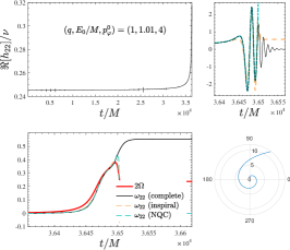
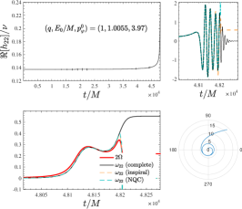
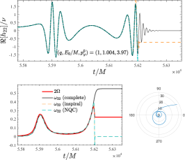
Figure 1: Waveform phenomenology for $q=1$: selected configuration to illustrate the transition from direct plunge (left panel) to one distinct encounter before the final merger (right panel). Each configuration is characterized by initial data $(q,E_{0}/M,p_{\varphi}^{0})$. The top row of each panel shows the real part of the $\ell=m=2$ waveform, completed with merger and ringdown (black online), with close ups onto the final merger part. The left-bottom panel exhibits the gravitational wave frequency, while the right-bottom the last part of the relative separation $r(\varphi)$. The panels also show: (i) the purely analytical EOB (inspiral) waveform and frequency (orange online); (ii) the waveform completed by NR-informed next-to-quasi-circular corrections (NQC, blue online). Note that the analytical EOB waveform accounts for the GW emission up to the largest peak of the orbital frequency $\Omega$ (red online). It is only after that this point is reached that the postmerger-ringdown description is attached, analogously to the quasi-circular case Damour and Nagar (2014b); Nagar et al. (2017, 2018, 2019, 2020).

II.2 Setup of initial data

The initial data setup for hyperbolic encounters/dynamical capture was already discussed in Ref. Damour et al. (2014). One proceeds as follows: (i) fix a value of the angular momentum $p_{\varphi}$ such that the local peak of the potential energy is larger than $1$ (see Fig. 3 of Ref. Damour et al. (2014) or Fig. 6 below); (ii) choose a value of the initial energy $E_{0}/M$; (iii) choose a value of the initial separation, that should be large, typically $r_{0}=10000$ (though sometimes we also use $r_{0}=1500$); (iv) solve Eq. (1) for $p_{r_{*}}$ with $H_{\rm EOB}=E_{0}$. Since at such large values of $r_{0}$ spin effects are negligible, we can simply consider the nonspinning version of Eqs. (2)-(3), with $r_{c}=r$ Damour and Nagar (2014b) to obtain $p_{r_{*}}$. To span the parameter space, we first fix $p_{\varphi}=p_{\varphi}^{0}$ and we then choose the initial energy between $E_{\rm max}/M$, the energy of the unstable circular orbit (i.e. the peak of the effective potential $A(1+p_{\varphi}^{2}u^{2})$) and $E_{\rm min}/M=H_{\rm EOB}(p_{\varphi}^{0},p_{r_{*}}=0,r_{0})/M$. As discussed below, the region of parameter space with $E_{0}\leq E_{\rm max}$ is the one with the most interesting phenomenology, i.e. with the possibility of having many close passages before merger. On the contrary, the regions with $E_{0}\geq E_{\rm max}$ always correspond to direct capture events. We will not discuss explicitly this phenomenology, though it is obviously also allowed by the formalism.

III Dynamical capture phenomenology

Let us now give a general overview of the properties of the relative dynamics and waveforms from dynamical capture as predicted by our EOB model. Note that we will mainly focus on the capture scenario and discuss in Sec. IV below the scattering scenario. To simplify the discussion, we start by considering the $q=1$, nonspinning case. To setup initial data, we consider values of the angular momentum $p_{\varphi}$ sufficiently larger than the LSO value, $p_{\varphi}^{LSO}$ so as to allow for the peak of the potential energy to be larger than one. For each value of $p_{\varphi}$ we select values of the energy between $(\hat{E}_{\rm min},\hat{E}_{\rm max})$ as mentioned above. At a qualitative level, for a given value of $p_{\varphi}^{0}$, as the energy is decreased from $\hat{E}_{\rm max}$, the system passes through the following stages: (i) direct capture/plunge; (ii) one, or more, close encounters before merger; (iii) close passage and scattering away. In practice, the detailed behavior as energy is decreased is more complicated, because, as $E\to 1$ the system moves from scattering configurations back to (many) close encounters that eventually end up with gravitational capture. More details on this phenomenology will be given below.

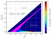
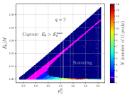
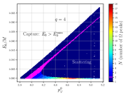
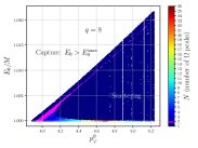
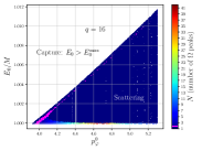
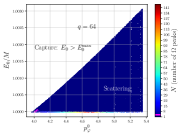
Figure 2: Analysis of the parameter space of hyperbolic encounters of nonspinning BBHs parameterized in terms of initial data $(q,E_{0}/M,p_{\varphi}^{0})$. The number of multiple encounters ($N\geq 2$) increases with $q$, while the corresponding area on the parameter space gets smaller and smaller. Note the separation, given by the colored area, between configurations that scatter and configurations that eventually merge.

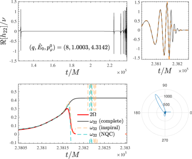
Figure 3: Extreme configuration with $(q,E_{0}/M,p_{\varphi}^{0})=(8,1.0003,4.3142)$ that undergoes eight periastron passages before merger. Note, after the first encounter, the very eccentric orbit, with apastron that reaches $r\simeq 1200$ (bottom left panel). Top right panel: close up on the final plunge, merger and ringdown part of the waveform. For completeness we also incorporate the purely analytical waveform (orange).

To start with, Fig. 1 shows three waveforms with nearly the same value of the angular momentum, but where the energy is progressively decreased. The configurations were selected so that one can appreciate the transition from immediate scattering (left panel) to a quasi-circular capture (middle panel), where the system does a full quasi-circular orbit before plunging, and the case when there’s a close encounter followed by capture and merger (right panel). For each configuration, we show: (i) the real part of the waveform; (ii) the gravitational wave frequency $\omega_{22}$ together with twice the orbital frequency $2\Omega$; and (iii) the orbit $r(\varphi)$ of the relative separation. For completeness, in both the waveform and frequency panels we include three curves: (i) the simple, analytical, EOB waveform, with the general Newtonian prefactor as explained in Ref. Chiaramello and Nagar (2020) (dashed, orange); (ii) the waveform corrected by additional next-to-quasi-circular (NQC) factors, that are informed by quasi-circular NR simulations following now standard procedures (light blue, dash-dotted) and the waveform completed with the, similarly NR-informed, ringdown. More precisely, the ringdown is attached at $t=2M$ after the peak of the $\ell=m=2$ analytic waveform, according to the standard procedure implemented in the various flavors of TEOBResumS Nagar et al. (2020); Chiaramello and Nagar (2020). To characterize the dynamics, it is useful to look at the morphology of the orbital frequency. In the case of immediate plunge, $\Omega=\dot{\varphi}$ has a single peak, corresponding to the crossing of the EOB effective light-ring. When the energy is lowered (see middle panel of Fig. 1), the frequency progressively flattens and an earlier peak appears well before the merger one. This “precursor” peak corresponds to a periastron passage with $r_{\rm periastron}\simeq 3.47$; after this, $r$ increases again and eventually the system plunges, with a second peak in $\Omega$. As the energy is further lowered (see third panel of Fig. 1), the first peak, that corresponds to the first close passage, becomes clearly distinguishable and separate from the one corresponding to merger. Inspecting the middle panel of Fig. 1, one then understands that the divide between having an immediate plunge and a close encounter followed by a plunge is determined by the condition $\dot{\Omega}=\ddot{\Omega}=0$, i.e. the orbital frequency should have an inflection point at some time (radius). Inspecting the left panel of Fig. 1, one sees how the late, inspiral-like, part of the orbit is fully mirrored by one entire GW cycles in the purely analytical waveform before the ringdown signal actually occurs. Similarly, in the middle panel one sees that the waveform mirrors the quasi-circular dynamics giving four, entire, GW cycles before merger and ringdown.

On the basis of the morphological analysis of above, a simple way to characterize the parameter space of dynamical capture is to focus on the orbital frequency as function of time, $\Omega(t)$, and count how many peaks are present. A single peak may correspond to either immediate plunge or scattering. More generally, when many peaks are present, each peak corresponds to a periastron passage. So, the number of peaks of $\Omega(t)$ is a simple observable, function of $(q,E_{0}/M,p_{\varphi}^{0})$ that could be used to characterize the parameter space of dynamical capture BBHs .

We then consider different mass ratios, $q=\{1,2,4,8,16,32,64,128\}$ to provide a comprehensive mapping of the parameter space. For each value of the angular momentum, we lower the energy and count the number of peaks of $\Omega$. The result of this analysis is reported in Fig. 2. The colors characterize how many periastron passages the system has undergone before merging. Focusing first on the $q=1$ case (top-left panel of the figure), one sees that when the energy is decreased from $\hat{E}_{\rm max}$ there are different islands of initial parameters that correspond to progressively more complicated physical behaviors. The plot is split in two by an area that corresponds to the frequency developing two peaks before merger (magenta online). As mentioned above, The upper boundary of this region is defined by those values of $(E_{0}/M,p_{\varphi}^{0})$ such that $\dot{\Omega}=\ddot{\Omega}=0$ at some time. Now, the $N=1$ part of the parameter space above the magenta region corresponds to direct plunge, with a waveform phenomenology similar to the one in the left panel of Fig. 1. By contrast, the $N=1$ part on the right and below the magenta region corresponds to scattering events instead of capture. When the initial energy is lowered further, getting close to the stability region, the system attempts to stabilize again and the number of periastron passages before merger increases progressively also for large values of $p_{\varphi}^{0}$. The phenomenology remains qualitatively the same also when the mass ratio is increased, but the region with $N=2$ becomes narrower and narrower as $q$ increases, notably for $q\geq 32$, when the divide between $N=1$ configuration is barely visible on the plots (we shall quantify this behavior better below). By contrast, for energies just slightly larger than the (adiabatic) stability limit, the number of possible encounters can grow considerably, up to several tens, although limited to a region of $p_{\varphi}^{0}$ much smaller than in the equal-mass case. We qualitatively interpret this behavior as mirroring the effect that radiation reaction, that is proportional to $\nu$, becomes less and less efficient as $\nu$ is decreased and so the system can persist in a metastable state much longer.

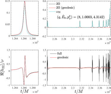
Figure 4: Importance of radiation reaction to determine the multiple-encounters behavior of Fig. 3, with the same initial conditions $(q,E_{0}/M,p_{\varphi}^{0})=(8,1.0003,4.3142)$ considered there. The black lines correspond to the full dynamics with radiation reaction, while the red ones correspond to the conservative dynamics alone.

In order to give an explicit example of the complicated phenomenology of a capture that occurs after many close encounters, let us consider a configuration with $(q,E_{0}/M,p_{\varphi}^{0})=(8,1.00026983016,4.3141870095)$, that is exhibited in Fig. 3. The top row of the figure shows the real part of the waveform, each burst corresponding to a close passage. Analogously to what done in Fig. 1, the close up of the waveform around merger (top-right panel) also includes the analytical EOB waveform (orange). The bottom row exhibits the time-evolution of the frequency around merger as well as the relative trajectory. It is remarkable that after the first encounter the system undergoes an extremely elliptic orbit, with apastron reaching $r\simeq 1200$, before being captured again. This behavior is determined by the action of radiation reaction around the first close encounter: in that situation the system emits a burst of radiation that eventually makes the orbit close again instead of scattering away. We prove this by setting up the EOB dynamics with the same initial data, but switching off radiation reaction, i.e. both $\hat{\cal F}_{\varphi}=\hat{\cal F}_{r_{*}}=0$. Figure 4 compares the orbital frequency and waveform of Fig. 3 with the waveform obtained from the conservative dynamics only. The location of the first burst, that corresponds to the first encounter, is essentially the same for both configurations, highlighting that the effect of radiation reaction is practically negligible up to that point. The differences in the waveform (and thus dynamics) occur later, consistently with the fact mentioned above that the effect of radiation reaction is localized around the periastron passage. In the top panel of the figure we also compare the full GW frequency, $\omega_{22}$ with twice the orbital frequency $\Omega$, to highlight that $\omega_{22}\neq 2\Omega$ because of the various noncircular effects occurring near the periastron. From this example one also argues that the span of the capture region in the parameter space depends on the details of the model for radiation reaction and may thus change if an improved version of the latter is implemented within the model . We will comment more on the issue of analytical uncertainty of the model, and the related importance of NR simulations as a benchmark, in Sec. IV below.

Finally, to put on a more quantitative ground the specific qualitative observations made so far, we compute, for each value $q=\{1,2,4,8,16,32,64,128\}$ the fraction $Y_{N}$ of events with $N$ encounters (where the $N$-th encounter corresponds to merger in case of final capture). Figure 5 exhibits this quantity versus $\nu=q/(1+q)^{2}$. Configurations with two encounters are always the most frequent ones, although their fraction quickly decreases below $10\%$ for $q>4$ ($\nu<0.16$).

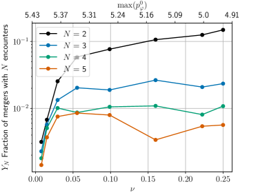
Figure 5: Fraction of BBH configurations (including also scattering events) that end up with $N$ encounters (where the $N$-th encounter corresponds to merger) for nonspinning binaries. Configurations with $N=2$ are the most frequent ones, although their frequency quickly decreases below $10\%$ as $q>4$ ($\nu<0.16$).

III.1 Spin

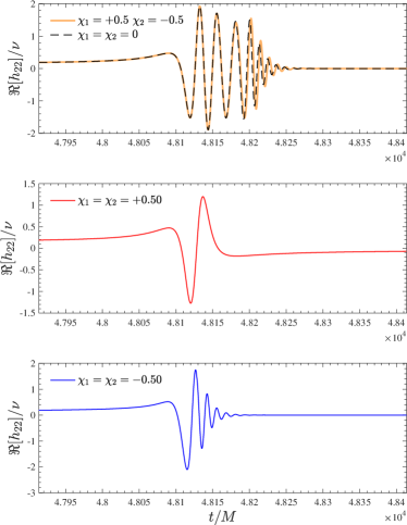
Figure 6: Effect of the spins on the $(q,E_{0}/M,p_{\varphi}^{0})=(1,1.0055,3.97)$ configuration discussed above. Top panel: when $\chi_{1}$ and $\chi_{2}$ are anti-aligned among themselves, the spin-orbit interaction cancels out and the waveform is almost equivalent to the nonspinning one. Middle panel: the repulsive character of spin-orbit interaction for spins aligned with the angular momentum is such to have a scattering instead of a dynamical capture. Bottom panel: when spins are anti-aligned with the angular momentum, the system plunges faster, with a short burst of radiation corresponding to the final capture.

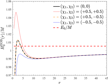
Figure 7: Potential energy $H^{\rm EOB}_{0}(r)/M$ for the four configurations shown in Fig. 6, that share the same $p_{\varphi}^{0}=3.97$ but have different values of the spins. The horizontal line corresponds to $E_{0}/M=1.0055$. The larger centrifugal barrier present when $\chi_{1}=\chi_{2}=+0.5$ is responsible of the scattering behavior in the middle panel of Fig. 6. In addition, the case $(\chi_{1},\chi_{2})=(+0.50,-0.50)$ is extremely close to $(\chi_{1},\chi_{2})=0$ because of spin-orbit coupling cancellation, consistently with the waveform shown in the top panel of Fig. 6.

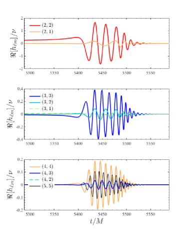
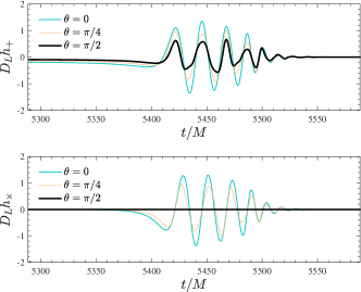
Figure 8: Calculation of higher modes for a nonspinning configuration with $(q,E_{0}/M,p_{\varphi}^{0})=(3.5,1.0067,4.1361)$. The phenomenology is qualitatively analogous to the $(q,E_{0}/M,p_{\varphi}^{0})=(1,1.0055,3.97)$ case shown in Fig. 1 above. $D_{L}h_{+}$ and $D_{L}h_{\times}$ waveform polarizations for $(q,E_{0}/M,p_{\varphi}^{0})=(3.5,1.0067,4.1361)$ at various inclinations: $\theta=0$ (face on), $\theta=\pi/4$ and $\theta=\pi/2$ (edge on). They are obtained combining the various multipoles showed using Eq. (7).

Let us turn now to discussing the effect of the spins (anti)aligned with the angular momentum. At a qualitative level, the waveform phenomenology is analogous to the nonspinning case considered above, though with some quantitative differences due to the spin-orbit and spin-spin interactions. We shall focus first on a special example to highlight the phenomenology. As mentioned above, due to the large initial separation the setup of initial data is insensitive to spin effects, so that the system can be consistently started with the same initial data setup for nonspinning binaries discussed above. In order to single out the effects of spins, we consider the same initial configuration $(q,E_{0}/M,p_{\varphi}^{0})=(1,1.0055,3.97)$ as above, with the following three choices for spins: $\chi_{1}=\chi_{2}=+0.50$; $\chi_{1}=\chi_{2}=-0.50$; $\chi_{1}=+0.50$ and $\chi_{2}=-0.50$. The corresponding waveforms are exhibited in Fig. 6. One clearly sees the following facts. When the BHs are spinning in opposite directions, the waveform is essentially equivalent to the nonspinning one. This is due to the well known cancellation of the spin-orbit interaction in the equal mass case, with the little differences in the waveforms predominantly due to spin-spin effects. To appreciate this at the level of dynamics, Fig. 7 shows that the potential energy $H^{\rm EOB}_{0}/M$ (i.e. Eq. (1) with $p_{r_{*}}=0$) for $(\chi_{1},\chi_{2})=(+0.50,-0.50)$ is visually indistinguishable from the nonspinning one. When the spins are both aligned with the orbital angular momentum, the centrifugal barrier is higher than in the nonspinning case (compare black and red lines in Fig. 7, and thus the system undergoes a scattering instead of a capture. The corresponding, burst-like, waveform is shown in the middle panel of Fig. 6. Finally, when spins are both anti-aligned with the orbital angular momentum, the spin-orbit interaction makes the attraction stronger than the nonspinning case (i.e. the potential barrier is much lower, see blue curve in Fig. 7) and the system plunges faster, with a signal whose pre-ringdown phase is much shorter than the nonspinning case.

III.2 Higher modes

Higher modes are incorporated in both the latest quasi-circular and eccentric realizations of TEOBResumS Nagar et al. (2019, 2020); Chiaramello and Nagar (2020). In the nonspinning case, all modes up to $\ell=m=5$ included are robustly completed by the NR-informed, quasi-circular, merger and ringdown part Nagar et al. (2019). By contrast, in the spinning case, due to numerical noise in the NR data, it was not possible to model the postmerger-ringdown part in modes modes like $(3,1)$, $(4,2)$ and $(4,1)$ (see Nagar et al. (2020)). Figure 8 shows, in the first three rows, several multipoles for $(q,E_{0}/M,p_{\varphi}^{0})=(3.5,1.0067,4.1361)$. For this choice of initial conditions, the system undergoes a quasi-circular orbit before plunge and merger, analogously to the corresponding $q=1$ case shown above in the middle panel of Fig. 1. One can appreciate that all modes can be obtained robustly with the standard ringdown matching procedure discussed in Refs. Nagar et al. (2019, 2020). For visual completeness, the last two rows of the figure also show the corresponding two polarizations $(h_{+},h_{\times})$, obtained using Eq. (7), for various inclinations.

IV EOB/NR scattering angle: the equal-mass case

Table 1: EOB scattering angle and comparison with the NR data of Ref. Damour et al. (2014). These results correspond to the standard configuration of the model, i.e. with 3PN-accurate $D$ and $Q$ functions. From left to right, the columns report: the configuration number; the minimum of the EOB radial separation (EOB impact parameter); the initial energy $\hat{E}^{0}$ and angular momentum $p_{\varphi}^{0}$; the NR and EOB energy losses; the NR and EOB angular momentum losses; the NR and EOB scattering angles and their fractional difference $\hat{\Delta}\chi^{\rm NREOB}\equiv|\chi^{\rm NR}-\chi^{\rm EOB}|/\chi^{\rm NR}$. Angles are measured in degrees. Note that, within the EOB, configuration $\#1$ does not scatter, but plunges instead.

#	$r_{\rm min}$	$\hat{E}^{0}$	$p^{0}_{\varphi}$	$\Delta E^{\rm NR}/M$	$\Delta E^{\rm EOB}/M$	$\Delta J^{\rm NR}/M^{2}$	$\Delta J^{\rm EOB}/M^{2}$	$\chi^{\rm NR}$	$\chi^{\rm EOB}$	$\hat{\Delta}\chi^{\rm NREOB}[\%]$
1	$\dots$	1.0225555(50)	4.3986080	0.01946(17)	0.032553	0.17007(89)	0.363750	305.8 (2.6)	$\dots$	$\dots$
2	3.70	1.0225722(50)	4.49039348	0.01407(10)	0.014083	0.1380(14)	0.134495	253.0(1.4)	279.35	10.4
3	4.03	1.0225791(50)	4.58209352	0.010734(75)	0.00951037	0.1164(14)	0.101919	222.9(1.7)	234.22	5.1
4	4.85	1.0225870(50)	4.8570920	0.005644(38)	0.0041582	0.076920(80)	0.0588254	172.0(1.4)	174.23	1.3
5	5.34	1.0225870(50)	5.0403920	0.003995(27)	0.00272826	0.06163(53)	0.045189	152.0(1.3)	153.01	0.7
6	6.49	1.0225884(50)	5.4986320	0.001980(13)	0.001172	0.04022(53)	0.027481	120.7(1.5)	120.79	0.07
7	7.59	1.0225924(50)	5.9568680	0.0011337(90)	0.0005951	0.029533(53)	0.018992	101.6(1.7)	101.51	0.09
8	8.66	1.0225931(50)	6.4150960	0.007108(77)	0.000332568	0.02325(47)	0.0141277	88.3(1.8)	88.19	0.12
9	9.72	1.0225938(50)	6.8733240	0.0004753(75)	0.00019778	0.01914(76)	0.0110359	78.4(1.8)	78.28	0.15
10	10.78	1.0225932(50)	7.33153432	0.0003338(77)	0.0001226	0.0162(11)	0.008928	70.7(1.9)	70.54	0.23

So far, we have investigated the analytical predictions of our EOB model for dynamical capture under the assumption that it provides a reasonably faithful representation of true signals. Evidently, seen the many approximations adopted to construct the model, a proof of this statement can only come from a systematic analysis of NR simulations of dynamical captures. Unfortunately, such NR simulations are currently not available. Despite this, we can actually test our model using some NR computation of the scattering angle previously published in Ref. Damour et al. (2014). The scattering angle, $\chi$, is the natural, gauge-invariant, observable that is used to characterize hyperbolic encounters. Reference Damour et al. (2014) provided the first measurement of $\chi$ from NR simulations and its comparison with an EOB prediction. The work of Ref. Damour et al. (2014) was a very preliminary investigation of a new territory and thus was limited to only $q=1$ binaries. Moreover, the EOB calculation of scattering angles of Ref. Damour et al. (2014) was not EOB-self consistent, since it was relying on energy and angular momentum losses computed from NR simulations. In this respect, Ref. Damour et al. (2014) allowed for a detailed analysis of the properties of the EOB Hamiltonian, but not of the full dynamical model. Now, thanks to the improved radiation reaction of Ref. Chiaramello and Nagar (2020), reliable in the strong field, we can finally go beyond the approach of Damour et al. (2014) and explore the reliability of the full model in hyperbolic encounters. This will allow us to put on a more solid ground the results discussed above. Reference Damour et al. (2014) considered 10 configurations, specified by Arnowitt-Deser-Misner (ADM) energy and angular momentum, of $q=1$ nonspinning black hole binaries. Each configuration was then evolved numerically. The initial data were chosen so as to always have a scattering and not a capture. Details of the NR simulations are reported in Table I of Damour et al. (2014). The values of the dimensionless initial ADM energy $E/M$ and dimensionless initial angular momentum $p_{\varphi}\equiv J/(M\mu)$ are now listed in the first column of Table 1. The seventh column of the table collects the values of the NR scattering angle, with their uncertainty, as published in Ref. Damour et al. (2014). As above, the initial EOB separation is chosen to be $r_{0}=10000$. The EOB values of the scattering angles are listed in the eight column of the table, while the last one lists fractional NR/EOB difference, $\hat{\Delta}\chi^{\rm NREOB}\equiv|\chi^{\rm NR}-\chi^{\rm EOB}|/\chi^{\rm NR}$. A few comments are in order: (i) the EOB/NR agreement between scattering angles is of the order of or below $1\%$ fractional difference except for three outliers that correspond, not surprisingly, to the smallest values of the impact parameter, although such fractional difference is within the NR uncertainty; (ii) for the first three configurations, the EOB model systematically overestimates the scattering angle, indicating that the system wants to be trapped and eventually plunge, instead of scatter away. This is indeed what happens for configuration $\#1$, where the system does a first close encounter, followed by a second one and the plunge.

Qualitatively speaking, this behavior is just mirroring the fact that the gravitational attraction as modeled within the EOB model is stronger than the actual NR prediction. At a more quantitative level, it is difficult to precisely quantify to which extent this is due to the conservative or nonconservative part of the dynamics. For what concerns the GW losses, columns 5-8 of Table 1 compare the total fraction of energy and angular momentum emitted in the NR simulation with the same quantity computed within the EOB formalism. This is what is accounted by the analytical fluxes entering the r.h.s. of Hamilton’s equation. The analytical fluxes are seen to always underestimate the numerical ones (sometimes also by $\sim 50\%$), except for configuration $\#2$. Despite this, the estimate of the scattering angle comes out consistent at a few percent level up to configuration $\#4$, thus suggesting the crucial importance of the conservative part of the dynamics. We shall come back to this point in the next section.

IV.1 Impact of beyond 3PN corrections in the $Q$ and $D$ EOB potentials

To have a deeper understanding of the results obtained above, let us first remember that Ref. Damour et al. (2014) showed that the best EOB/NR agreement was obtained by using a $D$ function at (incomplete) 4PN, that was taking into account only the linear-in-$\nu$ contributions available at the time Bini and Damour (2013). Now that the 4PN knowledge of the Hamiltonian is complete Damour et al. (2015, 2016), the 5PN information is complete except for two undetermined numerical parameters, $\bar{d}_{5}^{\nu^{2}}$ and $a_{6}^{\nu^{2}}$ , and similarly the 6PN is known except for four undetermined numerical parameters, $(q_{45}^{\nu^{2}},\bar{d}_{6}^{\nu^{2}},a_{7}^{\nu^{2}},a_{7}^{\nu^{3}})$ Bini et al. (2020b, c), it is worth to revive and improve the comparison of Ref. Damour et al. (2014). Note however that we do this here using the full model with radiation reaction and taking into account the contributions to either the $D$ and the $Q$ functions (while Ref. Damour et al. (2014) was just using the 3PN-accurate $Q$). In principle, we should also explore, within the present context, the effect of higher PN corrections to the $A$ function. However, we decided not to do so now for the following two reasons. On the one hand, the analytically known numerical value of the 5PN correction to the potential $a_{6}^{c}$ is such that the usual $(1,5)$ Padé approximant has a spurious pole, making thus this additional analytical knowledge practically useless within the current EOB context. Exploring different resummation strategies (e.g. changing Padé approximant) would be necessary in order to fruitfully use the analytically known 5PN result. On the other hand, we have verified that even large changes ($\sim 100\%$) of the NR-informed effective 5PN parameter $a_{6}^{c}(\nu)$ obtained in Refs. Nagar et al. (2019, 2020) and used here have little to negligible impact on the calculation of the scattering angle within the EOB model. This is consistent with the fact that the $A$ function rules the azimuthal part of the energy and it is less important in a hyperbolic-like context when the radial part of the Hamiltonian, i.e. $\propto p_{r_{*}}^{2}$ becomes predominant. To avoid additional complications we thus prefer to keep working with the NR-informed expression of the $A$ function used in previous work, focusing instead only on the high-PN corrections to the $Q$ and $D$ functions.

IV.1.1 Q function

Let us start discussing the $Q$ function. To simplify the logic, we keep $D$ fixed at 3PN order and consider only $Q$ at 4PN and at 5PN, though incorporating only local terms. The result of the $\chi$ computation is displayed in Table 2. One sees that the 4PN terms bring a small, though significative, contribution to the scattering angle that goes in the direction of reducing the EOB/NR difference. Despite this, the magnitude of the correction is too small to avoid configuration $\#1$ to plunge. By contrast, the effect of the 5PN local-in-time terms goes in the wrong direction and, moreover, is significantly smaller than the numerical uncertainty. At a practical level, and especially in view of the analytic complexity of the $Q$ function at 6PN, we don’t think it is worth, for the current study, to push $Q$ at 6PN accuracy and we shall just work, from now on, at 4PN accuracy in $Q$.

Table 2: Impact of 4PN and 5PN terms in the $Q$ function on the calculation of the scattering angle $\chi$. Angles are measured in degrees

#	$\chi^{\rm NR}$	$\chi^{\rm EOB}_{Q_{\rm 3PN}}$	$\chi^{\rm EOB}_{Q_{\rm 4PN}}$	$\chi^{\rm EOB}_{Q_{\rm 5PN}}$
1	305.8(2.6)	$\dots$	$\dots$
2	253.0(1.4)	279.35	278.21	278.75
3	222.9(1.7)	234.22	233.27	233.62
4	172.0(1.4)	174.23	173.57	173.72
5	152.0(1.3)	153.01	152.47	152.57
6	120.7(1.5)	120.79	120.44	120.49
7	101.6(1.7)	101.51	101.28	101.29
8	88.3(1.8)	88.19	88.03	88.04
9	78.4(1.8)	78.28	78.16	78.17
10	70.7(1.9)	70.54	70.44	70.45

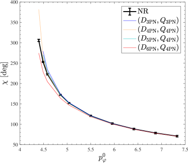
Figure 9: Comparing the NR scattering angles with various EOB predictions using different PN accuracies of the $(Q,D)$ potential. The 6PN-accurate $D$ function allows for the closest EOB/NR agreement for the smallest values of the EOB impact parameter.

Table 3: EOB scattering angle obtained using both $D$ and $Q$ functions and 4PN. The EOB/NR agreement is improved with respect to the standard case of Table 1 that adopt 3PN accuracy for these functions. Note that configuration $\#1$ does not plunge anymore.

#	$r_{\rm min}$	$\Delta E^{\rm EOB}/M$	$\Delta J^{\rm EOB}/M^{2}$	$\chi^{\rm NR}$	$\chi^{\rm EOB}$	$\hat{\Delta}\chi~{}[\%]$
1	3.31	0.022693	0.190585	305.8	381.93	24.89
2	3.71	0.012995	0.126256	253.0	264.21	4.43
3	4.03	0.008920	0.097128	222.9	225.12	0.99
4	4.85	0.003997	0.057269	172.0	170.53	0.85
5	5.34	0.002646	0.044311	152.0	150.60	0.92
6	6.49	0.001151	0.027202	120.7	119.72	0.81
7	7.59	0.000588	0.018878	101.6	100.93	0.66
8	8.66	0.000330	0.014074	88.3	87.85	0.51
9	9.72	0.000196	0.011008	78.4	78.05	0.44
10	10.78	0.000122	0.008912	70.7	70.38	0.45

Table 4: EOB scattering angle computed using $Q$ at 4PN and $D$ at 5PN, though resummed with a $(1,4)$ Padé approximant since $P^{0}_{5}$ develops a spurious pole.The EOB/NR agreement is worsened with respect to Table 3 and configuration $\#1$ plunges again. See text for discussion.

#	$r_{\rm min}$	$\Delta E^{\rm EOB}/M$	$\Delta J^{\rm EOB}/M^{2}$	$\chi^{\rm NR}$	$\chi^{\rm EOB}$	$\hat{\Delta}\chi~{}[\%]$
1	$\dots$	0.031705	0.347309	305.8	plunge	$\dots$
2	3.71	0.013463	0.129751	253.0	270.26	6.82
3	4.03	0.009161	0.099057	222.9	228.48	2.50
4	4.85	0.004054	0.057809	172.0	171.63	0.22
5	5.34	0.002673	0.044589	152.0	151.22	0.51
6	6.49	0.001157	0.027273	120.7	119.92	0.65
7	7.59	0.000590	0.018901	101.6	101.01	0.58
8	8.66	0.000330	0.014083	88.3	87.88	0.47
9	9.72	0.000197	0.011012	78.4	78.07	0.42
10	10.78	0.000122	0.008914	70.7	70.39	0.44

Table 5: EOB scattering angle computed using $D$ function at 6PN and the $Q$ function at 4PN Bini et al. (2020a, b). The 6PN-accurate $D$ function is essential to get an improved EOB/NR agreement for small values of the EOB impact parameter. Note, however, that this also brings slightly larger deviations with respect to the previous cases for intermediate values of $r_{\rm min}$.

#	$r_{\rm min}$	$\Delta E^{\rm EOB}/M$	$\Delta J^{\rm EOB}/M^{2}$	$\chi^{\rm NR}$	$\chi^{\rm EOB}$	$\hat{\Delta}\chi~{}[\%]$
1	3.33	0.015559	0.141465	305.8	274.68	10.18
2	3.71	0.010137	0.105088	253.0	228.49	9.69
3	4.03	0.007422	0.085263	222.9	204.52	8.24
4	4.85	0.003654	0.054047	172.0	163.99	4.66
5	5.34	0.002490	0.042707	152.0	146.99	3.30
6	6.49	0.001121	0.026816	120.7	118.63	1.71
7	7.59	0.000580	0.018755	101.6	100.51	1.07
8	8.66	0.000327	0.014027	88.3	87.66	0.72
9	9.72	0.000195	0.010987	78.4	77.96	0.56
10	10.78	0.000122	0.008902	70.7	70.33	0.52

IV.1.2 D function

Now that we have explored the (ir)relevance of the various PN truncations of the $Q$ function, let us move to exploring the $D$ function. We consider all terms up to 6PN, i.e. separately work with 4PN, 5PN and 6PN truncations, keeping the accuracy of $Q$ fixed at 4PN. Each $D$ function, that comes as a PN-truncated series, is resummed. Let us write here, for completeness, the Taylor expansion of $D$ up to 6PN

$$D^{\rm Taylor}_{\rm 6PN} =1-6\nu u^{2}-(52\nu-6\nu^{2})u^{3}+\nu d_{4}u^{4}$$

$$+\nu d_{5}u^{5}+\nu d_{5.5}u^{11/2}+\nu d_{6}u^{6},$$ (8)

The standard resummation procedure for this function is to take a $P^{0}_{n}$ approximant of this equation. This approach is now so standard that any analytical result is usually given in terms of the denominator, $\bar{D}$ function, where $\bar{D}\equiv 1/D$ (see e.g. Refs. Bini et al. (2019, 2020a, 2020b, 2020c)). The coefficients $(d_{4},d_{5},d_{5.5},d_{6})$ in Eq. IV.1.2 are obtained by just expanding $1/\bar{D}$ as given in the literature. One finds that the 5PN $D$ function resummed taking the $(0,5)$ Padé approximant has a spurious pole around $u\approx 0.5$ and thus it cannot be used robustly to deliver analytical prediction. That is the reason why we prefer to give the results of Refs. Bini et al. (2019, 2020a, 2020b, 2020c) in terms of the $D$ function in Eq. (IV.1.2) and then, at 5PN accuracy, proceed by resumming it with a $(1,4)$ Padé approximant, that is $D_{\rm 5PN}=P^{1}_{4}\left[D^{\rm Taylor}_{\rm 5PN}\right]$, that is found to have a pole-free behavior. The results of the calculations of the scattering angle with higher PN knowledge in $D$ are listed in Tables 3-5. The following conclusions are in order: (i) increasing the analytic information of $D$ to 4PN brings the first, important, qualitative and quantitative improvement, since configuration $\#1$ is found to correctly scatter (though the scattering angle is still significantly smaller than the NR one) instead of plunging; (ii) moving to 5PN is a step back, since configuration $\#1$ plunges again. By contrast, (iii), a remarkable improvement is obtained working at 6PN, retaining all the currently unknown numerical parameters fixed to zero. For the smallest impact parameters, the EOB/NR difference is at most of the order of $10\%$, an improvement of more than a factor two with respect to the cases discussed above. One also notes, however, that for intermediate values of the EOB impact parameter the EOB/NR agreement is slightly less good than, for instance, the $(D_{\rm 4PN},Q_{\rm 4PN})$ case.

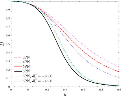
Figure 10: The resummed $D$ function for $q=1$ at various PN orders. The function gets progressively steeper as the PN order is increased. The orange lines corresponds to the flexed 6PN function where we put $d_{5}^{\nu^{2}}=-3500$ (dashed) and $d_{5}^{\nu^{2}}=-4500$ (dash-dotted). This latter brings the EOB/NR agreement of the order of percent for any configuration considered. See Table 6 and additional discussion in text.

Table 6: Tuned $D$ potential with $\bar{d}_{5}^{\nu^{2}}=-3500$. This number is chosen so to have an excellent EOB/NR agreement for configuration $\#1$. Still, for half of the configurations the EOB/NR difference is slightly larger than the NR error bar. See text for additional discussion.

#	$r_{\rm min}$	$\Delta E^{\rm EOB}/M$	$\Delta J^{\rm EOB}/M^{2}$	$\chi^{\rm NR}$	$\chi^{\rm EOB}$	$\hat{\Delta}\chi[\%]$
1	3.32	0.017860	0.157308	305.8	303.17	0.86
2	3.71	0.011289	0.113663	253.0	243.02	3.9
3	4.03	0.008109	0.090735	222.9	214.15	3.9
4	4.85	0.003853	0.055929	172.0	167.87	2.4
5	5.34	0.002591	0.043749	152.0	149.36	1.7
6	6.49	0.001145	0.027120	120.7	119.50	0.10
7	7.59	0.000587	0.018867	101.6	100.89	0.69
8	8.66	0.000330	0.014075	88.3	87.85	0.51
9	9.72	0.000197	0.011010	78.4	78.06	0.43
10	10.78	0.000122	0.008914	70.7	70.39	0.44

It is useful to visualize the functional behavior of the resummed $D$ function for the various PN orders considered above, see Fig. 10. The effect of higher PN order is to reduce the magnitude of the $D$ potential for $u\gtrsim 0.15$, i.e. $r\lesssim 7$. This is indeed the regime of radii explored by configurations $\#1-\#7$. The figure then indicates that the $D$ function that best approximates the NR values of the scattering angle (within the current analytical framework) should be slightly larger than the analytically known 6PN one, starting from $u\approx 0.18$. Still, it has to stay well below the 4PN curve. Although our finding is rather interesting because it demonstrates that, by varying a single analytical element, one can progressively improve the EOB/NR agreement of the scattering angle, it is not yet satisfactory because the difference is still larger than the NR error bar. It is then reasonable to ask whether it is possible to effectively flex the current $D_{\rm 6PN}$ so as to further improve the EOB/NR agreement for the smallest values of $r_{\rm min}$. As noted above $D_{\rm 6PN}$ is analytically known modulo three parameters, $(a_{6}^{\nu^{2}},\bar{d}_{5}^{\nu^{2}},\bar{d}_{6}^{\nu^{2}})$. We found that changing only $\bar{d}_{5}^{\nu^{2}}$ gives us enough flexibility for our aim. Figure 10 exhibits, with a orange line, the curve corresponding to $\bar{d}_{5}^{\nu^{2}}=-3500$. This value of the parameter was determined so to provide an EOB/NR agreement below the percent level for the smallest values of the impact parameter, as shown in Table 6. One should however note that for half of the configurations, the EOB/NR difference is still larger than the NR error bar, that is always of the order of percent or smaller. One then verifies that $\bar{d}_{5}^{\nu^{2}}=-4500$ allows one to obtain values of $\hat{\Delta}\chi=(2.52,2.07,2.57,1.73,1.13)\%$ for the first five configurations, and below $1\%$ for the following ones, i.e. $\hat{\Delta}\chi=(0.79,0.59,0.45,0.39,0.41)\%$. One should note, however, that $\chi_{\#1}^{\rm EOB}=313.51$, i.e. it is now larger than the NR value. The curve with $\bar{d}_{5}^{\nu^{2}}=-4500$ is also shown on Fig. 10 for completeness. Evidently, seen the still large errors in the NR computations, that date back to a few years ago, the various approximations involved in our analytical model (notably, the radiation reaction) and various possibilities of tuning free parameters, we do not want to make any strong claim about the physical meaning to the NR-tuning of $\bar{d}_{5}^{\nu^{2}}$. Still, our exercise shows that there is a large amount of yet unexplored analytical flexibility within the EOB model that can be constrained using the NR knowledge of the scattering angle, as originally advocated in Ref. Damour et al. (2014).

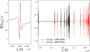
Figure 11: Waveforms for configuration with $(q,E_{0}/M,p_{\varphi}^{0})=(8,1.0003,4.3142)$ considered in Figs. 3 and 4 with $(D,Q)$ at 3PN (resummed) accuracy contrasted with the analytical prediction obtained with $D$ at 6PN and $Q$ at 4PN. The left panel compares the waveforms during the first encounter; the right panel the subsequent periastron passages, up to the final merger. The phenomenology is qualitatively the same, but the less attractive character of $D_{\rm 6PN}$ with respect to $D_{\rm 3PN}$ results in a larger time-lag between one encounter and the other and in a waveform that is globally almost twice longer.

As an additional exploratory study, we show in Fig. 11 how would change the waveform for $(q,E_{0}/M,p_{\varphi}^{0})=(8,1.0003,4.3142)$ of Fig. 3 when we replace $(D_{\rm 3PN},Q_{\rm 3PN})$ with $(D_{\rm 6PN},Q_{\rm 4PN})$. The less attractive character of $D_{\rm 6PN}$, as discussed above, results in a larger time-lag between the various bursts after the first encounter and the waveform is almost twice longer than with $D_{\rm 3PN}$ case. We conclude that there is a urgent need of specifically tuned NR simulations of dynamical capture black hole binaries aiming at understanding to which extent the analytical elements entering our model are trustable and what needs to be changed in order to achieve a level of NR-faithfulness sufficient for parameter-estimation purposes.

V Conclusions

We presented an EOB model to describe the dynamics of spin-aligned BBH hyperbolic encounters and the emitted gravitational waveform. The model generalizes the most developed version of TEOBResumS (named TEOBiResumS_SM) to dynamical captures, in particular building on the approach introduced in Ref. Chiaramello and Nagar (2020). The dynamics includes radiation reaction and multipolar waveforms for BBH with arbitrary mass ratio and aligned-spin interactions. Our main findings can be summarized as follows:

• We have extensively explored the parameter space of nonspinning dynamical captures, parameterizing it in terms of initial energy and angular momentum. In particular, we have characterized various regions on the basis of the number of close encounters that happen before merger, that are measured looking at the number of peak of the orbital frequency. We have found that the region of parameter space with two peaks, i.e. an encounter followed by the merger, gets smaller and smaller as the mass ratio increases. By contrast, the number of encounters before merger in the special region close to the stability regime increases with the mass ratio. The dynamical behavior mirrors in the waveform, that is completed with a merger and ringdown part informed by quasi-circular NR-simulation. The waveform incorporates multipoles up to $\ell=m=5$. Modes with $m=0$ are currently missing in the model.

• We have briefly explored the effect of spin, in order to get a qualitative idea of the general behavior. The effect of spins is essentially two fold. When spin are aligned with respect to the orbital angular momentum, a capture that is present in the nonspinning case, may transform in scattering if the spin-orbit interaction is sufficiently strong. By contrast, spins anti-aligned with the orbital angular momentum accelerate the capture process, so that the corresponding waveform eventually ends up with less gravitational wave cycles, and is dominated by the final ringdown part.

• Beyond the need, for GW-data purposes, of providing an analytical description of the dynamics and radiation of relativistic hyperbolic encounters, we have refreshed the EOB/NR comparison between scattering angles $\chi$ that was pioneered in Ref. Damour et al. (2014). Two are our most relevant findings. On the one hand, working with the $D$ function at 3PN, i.e. exactly with the eccentric EOB model of Ref. Chiaramello and Nagar (2020), we showed that an EOB-self-consistent calculation of the scattering angle (that is, including radiation reaction) is well compatible with the NR results of Ref. Damour et al. (2014), although things become quantitatively and qualitatively different (i.e. plunge instead of scattering) for the smallest value of the EOB impact parameter.

  On the other hand, we have systematically explored the impact of 4PN, 5PN and 6PN corrections to the $D$ function. Our most important finding is that the recently computed, 6PN-accurate, $D$ function allows one to obtain an EOB/NR agreement for the scattering angle of a few percents also for the configurations with the smallest impact parameter. We thus argue that our model for hyperbolic scattering/dynamical capture is, probably, more accurate using $D_{\rm 6PN}$ instead of $D_{\rm 3PN}$. Still, one has to mention that the improvement for small values of $r_{\rm min}$ is balanced by a slight worsening of the $\chi$ computation for intermediate values of the impact parameter. Due to the absence of additional NR simulations all over the parameter space, we take the difference between $D_{\rm 3PN}$ and $D_{\rm 6PN}$ results as a (rather conservative) error bar that might be taken into account, using the current model, in a possible parameter estimation on a GW detection qualitatively and morphologically compatible with a dynamical capture scenario.

  We have also shown that it is rather easy to additionally tune the $D_{\rm 6PN}$ function so as to further improve the EOB/NR agreement of the scattering angle, at the level of the actual estimate of the uncertainty on the NR scattering angle. This is done by tuning only the uncalculated 5PN numerical parameter $\bar{d}_{5}^{\nu^{2}}$. Concretely, our results indicate that, one the one hand, it would be a good idea to incorporate the 6PN-accurate $D$ function in waveform model for quasi-circular coalescing BBHs; on the other hand, it proves that NR simulations of the scattering angle can be used to inform the EOB model and thus dedicated NR simulations to systematically and usefully explore the parameter space should be performed at some stage. Similarly, systematic NR surveys of dynamical capture are needed to test our model and to possibly improve the merger-ringdown part, that at the moment is informed by quasi-circular simulations. Also, dedicated simulations in the large-mass-ratio limit, e.g. using Teukode Harms et al. (2014), would be needed to provide strong tests of the model at a moderate computational cost. This investigation will be pursued in future work. This strategy seems the only viable at the moment in order to complete a multi-purpose EOB-based waveform model able to take into account any kind of coalescence configuration, from quasi-circular ones, to eccentric up to dynamical capture.

Our waveform model is implemented as a standalone $C$ code that is publicly available via a bitbucket repository teo . Details of the implementation are also discussed in Ref. Chiaramello and Nagar (2020). Its performance for parameter estimation and optimization is under way and will be reported in a separate publication. We finally note that the recently published GW signal GW190521 Abbott et al. (2020a, b), though interpreted as a BBH coalescence with total mass $M\simeq 142M_{\odot}$ using precessing, quasi-circular, templates, has a morphology compatible with that of a dynamical capture. As advocated in Ref. CalderF3n Bustillo et al. (2020) (see also Romero-Shaw et al. (2020); Gayathri et al. (2020)), our model could be used in the future to attempt to rule out that GW190521 is actually the result of a dynamical capture BBH merger.