Tiling with triangles: parquet and $GW\gamma$ methods unified

Abstract

The parquet formalism and Hedin’s $GW\gamma$ approach are unified into a single theory of vertex corrections, corresponding to an exact reformulation of the parquet equations in terms of boson exchange. The method has no drawbacks compared to previous parquet solvers but has the significant advantage that the vertex functions decay quickly with frequencies and with respect to distances in real space. These properties coincide with the respective separation of the length and energy scales of the two-particle correlations into long/short-ranged and high/low-energetic.

I Introduction

The systematic calculation of vertex corrections in electronic systems historically builds upon two distinct formalisms, the parquet formalism of De Dominicis and Martin De Dominicis and Martin (1964a) (introduced also earlier by Diatlov et al. for meson scattering Diatlov et al. (1957)) and the $GW\gamma$ method introduced by Hedin Hedin (1965). Although both approaches are in widespread use since the 1960’s, they have largely remained separate entities.

The parquet approach Bickers (2004); Tam et al. (2013); Rohringer et al. (2012); Valli et al. (2015); Li et al. (2016, 2019); Astretsov et al. (2020) classifies vertex corrections into three scattering channels, allowing an unbiased competition between the bosonic fluctuations in these channels Friederich et al. (2011); Metzner et al. (2012); Tagliavini et al. (2019); Kauch et al. (2019); Pudleiner et al. (2019). The Hedin equations, on the other hand, aim at the particle-hole channel, with vertex corrections $\gamma$ in this channel being calculated self-consistently from the derivative of the self-energy with respect to the Green’s function $\delta\Sigma/\delta G$ Onida et al. (2002); Held et al. (2011). Both formalisms constitute an exact quantum field theoretical framework, but in practice one relies on approximations: In the case of the parquet formalism, the fully irreducible vertex $\Lambda$ is approximated, e.g., by $\Lambda=U$ (the bare interaction) in the parquet approximation Bickers (2004) or by $\Lambda={\rm local}$ in the dynamical vertex approximation Toschi et al. (2007); Katanin et al. (2009); Rohringer et al. (2018). In the case of the Hedin approach, $\gamma$ is approximated, e.g., by $\gamma=1$ in the $GW$ approximation or by simple approximations in so-called $GW\gamma$ approaches, even allowing for realistic materials calculations Godby et al. (1988); Aryasetiawan and Gunnarsson (1998); Onida et al. (2002); Biermann et al. (2003); Held et al. (2011); Tomczak et al. (2017); Nilsson et al. (2017); Maggio and Kresse (2017).

One difference is that the parquet formalism is formulated in terms of four-point electron-electron vertices (Feynman diagrammatic “squares”, capitalized symbols in our notation), whereas Hedin Hedin (1965) formulated his equations in terms of three-point electron-boson vertices (“triangles”, lowercase symbols). The latter can be reformulated easily in terms of four-point squares, see e.g. Held et al. (2011), but to the best of our knowledge the parquet approach evaded hitherto a three-point (triangle) reformulation.

A second major difference between the two approaches is that the parquet equations naturally obey the crossing symmetry but typical approximations violate conservation laws Smith (1992); Janiš (1999); Bickers (2004); Janiš and Kolorenč (2005); Janiš et al. (2017); Rohringer et al. (2018); Kugler and von Delft (2018); Krien (2018), whereas $GW\gamma$ approximations conversely often obey conservation laws Almbladh et al. (1999) but violate the crossing symmetry, and thereby the Pauli principle. Indeed, only the exact solution satisfies the crossing symmetry and the Ward identity at the same time, see Ref. Kugler and von Delft (2018) for a formal proof.

Aspects of both concepts come into play in the theory of collective bosonic fluctuations in fermionic systems, see, for example, Ref. Chubukov and Wölfle (2014), in particular of those in superconductors Larkin and Varlamov , where the three-legged fermion-boson coupling and the screened interaction are used to construct four-point vertex corrections. However, these considerations are almost always of a phenomenological kind and only a few Feynman diagrams of interest are calculated, such as the Aslamazov-Larkin vertex correction Aslamasov and Larkin (1968); Bergeron et al. (2011) (see diagram (b) in Fig. 3 below). But in terms of an overarching theory the relation between the parquet and Hedin formalisms remains, even after more than 50 years, only a tentative one.

In this paper, both approaches and viewpoints are merged into a single theory. It is shown that the parquet decomposition of the vertex function, which relies on the reducibility with respect to Green’s functions Rohringer et al. (2012), can be combined with the recently introduced single-boson exchange (SBE) decomposition Krien et al. (2019) that is based on the idea of reducibility with respect to the interaction, which generalizes the Hedin equations. In particular, the diagrams that are reducible with respect to the interaction can be removed exactly from the parquet expressions and suitable ladder equations can be defined which replace the Bethe-Salpeter equations. Through this exact reformulation of the parquet method, we tile our diagrammatic “floor” not with conventional four-leg parquet “squares” but with three-leg “triangles”, with the exception being an irreducible “square” $\tilde{\Lambda}=\Lambda-U$, which vanishes in the parquet approximation.

The present paper is in close conjunction with Ref. Krien et al. (2020a) where the parquet equations for dual fermions Rubtsov et al. (2008) have been reformulated. Instead, here we show how the standard parquet approach Bickers (2004); Tam et al. (2013); Rohringer et al. (2012); Valli et al. (2015); Li et al. (2016, 2019); Astretsov et al. (2020) can be rewritten and connected with the Hedin equations. As a result, the self-energy of the parquet approach assumes the “$GW\gamma$” form, which is not the case for the parquet dual fermions Krien et al. (2020b). An efficient real fermion parquet solver for a quantum impurity model is presented and made available Krien (2020). Similar as for dual fermions Krien et al. (2020a), this reformulation leads to a substantially improved feasibility of the parquet solution because it removes simultaneously the high-frequency asymptotics Wentzell et al. (2020) and the long-ranged fluctuations Rohringer et al. (2018) from the parquet equations.

The paper is organized as follows. The Hedin and parquet formalisms are recollected in Sections II and III, respectively. The two concepts are connected and merged in Section IV. A unified calculation scheme using the SBE decomposition is presented in Section V; and Section VI presents the implementation for a quantum impurity model (Section VI.1) and examples for the lattice Hubbard model from the parquet approximation (Section VI.2) using the victory code Li et al. (2019). Further, in Section VI.3, we reduce the results of the parquet approximaton step-by-step to the $GW$ approximation. We conclude in Sec. VII, where we also discuss similarities and differences of the method compared to the one presented in Ref. Krien et al. (2020a).

II Hedin’s formalism

In Hedin’s theory the self-energy of the electronic system is expressed in terms of the Green’s function $G$, the screened interaction $W$, and the vertex $\gamma$. For a single-band Hubbard-type system with the interaction $Un_{\uparrow}n_{\downarrow}$ the self-energy can be expressed in the paramagnetic case as follows :

$$\Sigma_{k}=\frac{U\langle n\rangle}{2}-\frac{1}{2}\sum_{q}G_{k+q}\left[W^{\text{ch}}_{q}\gamma^{\text{ch}}_{kq}+W^{\text{sp}}_{q}\gamma^{\text{sp}}_{kq}\right].$$ (1)

Here, ch and sp denote the charge and spin (or density and magnetic) combinations of the spin indices, respectively, see e.g. Rohringer et al. (2018); $\langle n\rangle$ is the density; $k=(\mathbf{k},\nu)$ and $q=(\mathbf{q},\omega)$ denote fermionic and bosonic momentum-energy four-vectors, respectively, $\nu,\omega$ are Matsubara frequencies. Summations over $k,q$ imply a factor $T,\frac{1}{N}$ where $T$ is the temperature and $N$ the number of lattice sites. The Hedin vertex $\gamma^{\text{ch}(\text{sp})}$ takes, in the exact theory, all vertex corrections in the particle-hole channel into account.

The screened interaction $W$ corresponds to the bare Hubbard interaction $U^{\text{ch}}=U,U^{\text{sp}}=-U,U^{\text{s}}=2U,U^{\text{t}}=0$ in the charge (ch) and spin (sp), singlet (s), triplet (t) channel, respectively, dressed by the polarization $\Pi$, i.e.,

$$W^{\text{ch}/\text{sp}}_{q}=\frac{U^{\text{ch}/\text{sp}}}{1-U^{\text{ch}/\text{sp}}\Pi^{\text{ch}/\text{sp}}_{q}},\;\;\;W^{\text{s}}_{q}=\frac{U^{\text{s}}}{1-\frac{1}{2}U^{\text{s}}\Pi^{\text{s}}_{q}}.$$ (2)

For later use, we here introduced a $W^{\text{s}}$ also for the singlet particle-particle channel, while $W^{\text{t}}=0$. Both are not used in Hedin’s original $GW\gamma$ approach, but are needed for the later connection to the parquet approach, which includes the particle-particle channel. The third, transversal particle-hole, channel is related to the particle-hole channel by crossing symmetry. Hence we do not need to introduce two further $W$’s and $\gamma$’s; $W^{\text{ch}(\text{sp})}$ and $\gamma^{\text{ch}(\text{sp})}$ in the particle-hole channel are sufficient.

The polarization in Eq. (2) is in turn given by the Hedin vertex:

$$\Pi^{\text{ch}/\text{sp}}_{q}=\sum_{k}G_{k}G_{k+q}\gamma^{\text{ch}/\text{sp}}_{kq},\Pi^{\text{s}}_{q}=\sum_{k}G_{k}G_{q-k}\gamma^{\text{s}}_{kq}.$$ (3)

Equations (1)-(3) are formally exact, but in general the vertex corrections contained in $\gamma$ are unknown. Hedin Hedin (1965) suggested to calculate these through the Ward identity (see also Sec. V) but this is hardly feasible in practice. Instead, the vertex corrections $\gamma$ are often neglected which gives rise to the eponymous $GW$ approximation. If (some approximate) vertex corrections are kept one speaks of a $GW\gamma$ approach Del Sole et al. (1994).

The diagrammatic background to introduce $W$ and $\Pi$ in the Hedin equations is the concept of interaction-(ir)reducibility: a Feynman diagram is interaction-reducible if and only if it separates into two pieces if one interaction line is cut out. Eventually, we need to consider all vertex corrections, i.e., the full vertex function $F^{\alpha}_{kk^{\prime}q}$. The interaction-reducible diagrams of $F$ take the form Krien et al. (2019),

$$\Delta^{\alpha}_{kk^{\prime}q}=\gamma^{\alpha}_{kq}W^{\alpha}_{q}\gamma^{\alpha}_{k^{\prime}q}.$$ (4)

Quite obviously, we can cut an interaction line $U$ within $W$ and hence $\Delta$, and vice versa any interaction-reducible diagram in channel $\alpha$ has to be of the form Eq. (4). The vertex $\Delta$ has been coined single-boson exchange (SBE) vertex Krien et al. (2019) as it involves the exchange of a single boson with four-vector $q$ within $W$.

These interaction-reducible contributions must not be contained in $\gamma$, and hence must be subtracted from $F$ to avoid a double counting . This yields Krien et al. (2019):

$$\gamma^{\text{ch}/\text{sp}}_{kq}= 1+\sum_{k^{\prime}}(F^{\text{ch}/\text{sp}}_{kk^{\prime}q}-\Delta^{{\text{ch}/\text{sp}}}_{kk^{\prime}q})G_{k^{\prime}}G_{k^{\prime}+q},$$ (5a)

$$\gamma^{\text{s}}_{kq}= -1+\frac{1}{2}\sum_{k^{\prime}}(F^{\text{s}}_{kk^{\prime}q}-\Delta^{\text{s}}_{kk^{\prime}q})G_{k^{\prime}}G_{q-k^{\prime}}.$$ (5b)

Here, the Green’s functions serve the conversion of the four point vertex $F-\Delta$ to the three point vertex $\gamma$, and the “1” generates in the Hedin formulations the contributions without vertex corrections. There is no triplet Hedin vertex because the bare interaction vanishes in this channel, $U^{\text{t}}=0$.

III Parquet formalism

The parquet formalism De Dominicis and Martin (1964b, a); Bickers (2004); Gunnarsson et al. (2016); Rohringer et al. (2018) is based on the insight that the full vertex $F$ can be decomposed into the fully-irreducible vertex $\Lambda$ and reducible vertices $\Phi^{r}$ in the particle-hole ($r=ph$), transversal-particle-hole ($r=\overline{ph}$) and particle-particle-channel ($r=pp$). Now (two-particle) irreducibility is to be understood with respect to cutting two Green’s function lines. Each Feynman diagram for $F$ belongs to exactly one of these four classes, i.e., $F=\Lambda+{\Phi}^{ph}+{\Phi}^{\overline{ph}}+{\Phi}^{pp}$ Bickers (2004); Rohringer et al. (2018). In terms of the spin combinations $\alpha=\text{ch},\text{sp}$, we get with the momentum-convention for the particle-hole channel (cf. Fig. 1, left),

$$F^{\alpha}_{kk^{\prime}q}= {\Lambda}^{\alpha}_{kk^{\prime}q}+{\Phi}^{ph,\alpha}_{kk^{\prime}q}$$ (6)

$$- \frac{1}{2}{\Phi}^{ph,\text{ch}}_{k,k+q,k^{\prime}-k}-\frac{3-4\delta_{\alpha,\text{sp}}}{2}{\Phi}^{ph,\text{sp}}_{k,k+q,k^{\prime}-k}$$

$$+ \frac{1-2\delta_{\alpha,\text{sp}}}{2}{\Phi}^{pp,\text{s}}_{kk^{\prime},k+k^{\prime}+q}+\frac{3-2\delta_{\alpha,\text{sp}}}{2}{\Phi}^{pp,\text{t}}_{kk^{\prime},k+k^{\prime}+q}.$$

Here, we have expressed $\Phi^{\overline{ph}}$ in terms of $\Phi^{{ph}}$ in the second line using the crossing relation Rohringer et al. (2012), and properly translated the s and t components and momenta of the $pp$ channel in the third line. The fully irreducible vertex ${\Lambda}$ or an approximation thereof, such as the parquet approximation ${\Lambda}^{\alpha}=U^{\alpha}$, serves as an input.

Since $\alpha=\text{ch},\text{sp}$ and $\alpha=\text{s},\text{t}$ already uniquely determine the channel $r=ph$ and $r=pp$, respectively, we drop the channel index $r$ in the following.

There is only one $F$ with two independent spin combinations, but one can use the singlet and triplet combinations and $pp$ momentum convention (cf. Fig. 1), which is related to the above by

$$F^{\text{s}}_{kk^{\prime}q}= \frac{1}{2}\left(F^{\text{ch}}_{kk^{\prime},q-k-k^{\prime}}-3F^{\text{sp}}_{kk^{\prime},q-k-k^{\prime}}\right),$$ (7a)

$$F^{\text{t}}_{kk^{\prime}q}= \frac{1}{2}\left(F^{\text{ch}}_{kk^{\prime},q-k-k^{\prime}}+F^{\text{sp}}_{kk^{\prime},q-k-k^{\prime}}\right).$$ (7b)

One can further introduce an irreducible vertex in the respective channel

$${\Gamma}^{\alpha}_{kk^{\prime}q}=F^{\alpha}_{kk^{\prime}q}-{\Phi}^{\alpha}_{kk^{\prime}q}.~{}$$ (8)

Figure 1: Label convention for (a) the particle-hole and (b) the particle-particle notation.

For calculating the reducible vertices, we employ the Bethe-Salpeter equations which in terms of $\Phi$ read

$${\Phi}^{\text{ch}/\text{sp}}_{kk^{\prime}q}= \sum_{k^{\prime\prime}}{\Gamma}^{\text{ch}/\text{sp}}_{kk^{\prime\prime}q}G_{k^{\prime\prime}}G_{k^{\prime\prime}+q}F^{\text{ch}/\text{sp}}_{k^{\prime\prime}k^{\prime}q},$$ (9a)

$${\Phi}^{\text{s}/\text{t}}_{kk^{\prime}q}= \mp\frac{1}{2}\sum_{k^{\prime\prime}}{\Gamma}^{\text{s}/\text{t}}_{kk^{\prime\prime}q}G_{k^{\prime\prime}}G_{q-k^{\prime\prime}}F^{\text{s}/\text{t}}_{k^{\prime\prime}k^{\prime}q}.$$ (9b)

Here, we can replace ${\Gamma}$ by Eq. (8), which allows for a self-consistent calculation of $\Phi$ and $F$ in the four-channels if $\Lambda$ is known as an input. Further, $G$ and $\Sigma$ can be calculated self-consistently as well, using additionally the Dyson equation and Schwinger-Dyson equation [that is equivalent to Eq. (1)].

IV A unified approach to vertex corrections

We now relate the Hedin and parquet formalisms described in Sections II and III. Starting point is an analog to the parquet Eq. (6) but formulated in terms of interaction-(ir)reducible vertices instead of the two-particle (ir)reducibility of Eq. (6). This SBE decomposition Krien et al. (2019) into interaction-reducible channels reads for $\alpha=\text{ch},\text{sp}$:

$$F^{\alpha}_{kk^{\prime}q}= {\Lambda}^{\text{Uirr},\alpha}_{kk^{\prime}q}+{\Delta}^{\alpha}_{kk^{\prime}q}$$ (10)

$$- \frac{1}{2}{\Delta}^{\text{ch}}_{k,k+q,k^{\prime}-k}-\frac{3-4\delta_{\alpha,\text{sp}}}{2}{\Delta}^{\text{sp}}_{k,k+q,k^{\prime}-k}$$

$$+ \frac{1-2\delta_{\alpha,\text{sp}}}{2}{\Delta}^{\text{s}}_{kk^{\prime},k+k^{\prime}+q}-2U^{\alpha}.$$

The essential difference to the parquet Eq. (6) is that the vertices $\Delta^{\alpha}$ defined in Eq. (4) are reducible with respect to the bare interaction $U^{\alpha}$ . The bare interaction is itself interaction-reducible and hence included in the $\Delta^{\alpha}$’s; thus we need to subtract $2U^{\alpha}$ in Eq. (10) to prevent an overcounting. As already discussed in Section II, $U^{\text{t}}=W^{\text{t}}=\Delta^{\text{t}}=0$.

This also implies $\Lambda^{\text{Uirr}}$ is fully irreducible with respect to the interaction, and must not be confused with the vertex $\Lambda$ of the parquet decomposition Eq. (6) which is fully irreducible with respect to pairs of Green’s functions. This implies on the one hand that $U$ is contained in $\Lambda$ but not in $\Lambda^{\text{Uirr}}$. But otherwise $\Lambda$ contains fewer diagrams than $\Lambda^{\text{Uirr}}$ as each diagram that is interaction reducible is also two-particle reducible since we can cut the two Green’s functions on one side of the two-particle interaction instead of the interaction itself .

In the following we will relate the parquet equation (6) and the SBE generalization Eq. (10) of the Hedin formalism, and formulate a unified theory. To this end, we will pinpoint the difference between $\Lambda^{\text{Uirr}}$ and $\Lambda$, which is denoted as Krien et al. (2020a) multi-boson exchange (MBE) diagrams $M^{\alpha}$ (the SBE diagrams $\Delta^{\alpha}$ are not part of $\Lambda^{\text{Uirr}}$; Fig. 3 below clarifies the multi-boson character of $M$). We will derive the equations to calculate $M^{\alpha}$ and $\Delta^{\alpha}$ self-consistently in a unified Hedin and parquet formalism. This approach, while fully equivalent to the parquet approach, is formulated with the Hedin vertices and screened interactions and bears the advantage that the calculated vertex functions $\Lambda^{\text{Uirr}},M$ decay with the frequencies and depend only weakly on the momenta, compared to $F,\Phi$ of the original parquet approach.

First, we start with some definitions. Analogously to $\Gamma^{\alpha}$ in Eq. (8), we introduce vertices $T^{\alpha}$ that are irreducible with respect to the bare interaction $U^{\alpha}$ only in a particle-hole channel ($\alpha=\text{ch},\text{sp}$ ) or in a particle-particle channel ($\alpha=\text{s},\text{t}$) by removing the reducible diagrams ${\Delta}^{\alpha}$ in that channel:

$${T}^{\alpha}_{kk^{\prime}q}= F^{\alpha}_{kk^{\prime}q}-{\Delta}^{\alpha}_{kk^{\prime}q}.$$ (11)

By comparison with Eqs. (5a) and (5b) we see that the vertices $T$ describe the vertex corrections for the Hedin vertex $\gamma$. The latter is therefore also irreducible with respect to the bare interaction in the corresponding channel Krien et al. (2019); Rohringer and Toschi (2016).

As is the custom in Hedin’s formalism we remove the bare interaction $U^{\alpha}$ from the irreducible vertex $\Gamma^{\alpha}$:

$$S^{\alpha}=\Gamma^{\alpha}-U^{\alpha}.~{}$$ (12)

Now we collect all diagrams that are interaction-irreducible (but two-particle reducible) as the difference

$${M}^{\alpha}_{kk^{\prime}q}=T^{\alpha}_{kk^{\prime}q}-S^{\alpha}_{kk^{\prime}q}.~{}$$ (13)

Conversely, this means that $\Phi^{\alpha}$ consists of ${M}^{\alpha}$ plus the interaction-reducible vertices $\Delta^{\alpha}$ in the respective channel,

$$\Phi^{\alpha}_{kk^{\prime}q}=F^{\alpha}_{kk^{\prime}q}-\Gamma^{\alpha}_{kk^{\prime}q}=\Delta^{\alpha}_{kk^{\prime}q}-U^{\alpha}+{M}^{\alpha}_{kk^{\prime}q}.$$ (14)

Here again $U^{\alpha}$ needs to be subtracted as it is included in $\Delta^{\alpha}$ but not in $\Phi^{\alpha}$. A diagrammatic representation of Eq. (14) is shown in Fig. 2 for the particle-hole channel. Note that $\Phi^{\text{t}}=M^{\text{t}}$ since $U^{\text{t}}=\Delta^{\text{t}}=0$.

Figure 2: Relation Eq. (14) between the particle-hole reducible vertices $\Phi$ in Eq. (9a) and $M$ defined in Eq. (17a), which represents multi-boson exchange (cf. Fig. 3). Arrows and a dashed line denote Green’s function $G$ and the bare interaction $U$, respectively.

With these definitions, we can now relate $\Lambda^{\text{Uirr},\alpha}$ of the SBE decomposition Eq. (10) to ${\Lambda}^{\alpha}$ of the parquet Eq. (6), or more specifically to

$$\tilde{\Lambda}^{\alpha}={\Lambda}^{\alpha}-U^{\alpha}.$$ (15)

To this end, we equate Eq. (10) to Eq. (6), which both yield $F^{\alpha}$, and express $\Phi^{\alpha}$ by $M^{\alpha}$ using Eq. (14). We are left with

$$\Lambda^{\text{Uirr},\alpha}_{kk^{\prime}q}= \tilde{\Lambda}^{\alpha}_{kk^{\prime}q}+{M}^{\alpha}_{kk^{\prime}q}$$ (16)

$$- \frac{1}{2}{M}^{\text{ch}}_{k,k+q,k^{\prime}-k}-\frac{3-4\delta_{\alpha,\text{sp}}}{2}{M}^{\text{sp}}_{k,k+q,k^{\prime}-k}$$

$$+ \frac{1-2\delta_{\alpha,\text{sp}}}{2}{M}^{\text{s}}_{kk^{\prime},k+k^{\prime}+q}+\frac{3-2\delta_{\alpha,\text{sp}}}{2}{M}^{\text{t}}_{kk^{\prime},k+k^{\prime}+q}.$$

All $\Delta^{\alpha}$’s cancel, as it must be.

We still need to calculate the ${M}^{\alpha}$’s. This can be done through Bethe-Salpeter-like equations similar as the ${\Phi}^{\alpha}$’s in Eq. (9) of the original parquet formalism. Starting with Eq. (9), substituting $F^{\alpha}$, $\Gamma^{\alpha}$ and $\Phi^{\alpha}$ by Eqs. (11), (12), and (14), respectively, and removing all interaction-reducible contributions from the left and right hand side, this yields

$${M}^{\text{ch}/\text{sp}}_{kk^{\prime}q}= \sum_{k^{\prime\prime}}{S}^{\text{ch}/\text{sp}}_{kk^{\prime\prime}q}G_{k^{\prime\prime}}G_{k^{\prime\prime}+q}T^{\text{ch}/\text{sp}}_{k^{\prime\prime}k^{\prime}q},$$ (17a)

$${M}^{\text{s}/\text{t}}_{kk^{\prime}q}= \mp\frac{1}{2}\sum_{k^{\prime\prime}}{S}^{\text{s}/\text{t}}_{kk^{\prime\prime}q}G_{k^{\prime\prime}}G_{q-k^{\prime\prime}}T^{\text{s}/\text{t}}_{k^{\prime\prime}k^{\prime}q}.$$ (17b)

Here, $T=S+M$ [Eq.(13)] can be substituted.

Besides this Bethe-Salpeter equation, we need the eponymous parquet equation, i.e., Eq. (6) in the original parquet formalism. Moving $\Phi^{\alpha}$ for the considered four channels ($\alpha$) to the left hand side in Eq. (6) and reexpressing everything in terms of the new variables ($\Lambda^{\text{Uirr}},M,\Delta$), we obtain, analogous to Ref. Krien et al. (2020a), the parquet equation formulated in terms of

$${S}^{\text{ch}}_{kk^{\prime}q}=\, {\Lambda}^{\text{Uirr},\text{ch}}_{kk^{\prime}q}-{M}^{\text{ch}}_{kk^{\prime}q}-\frac{1}{2}{\Delta}^{\text{ch}}_{k,k+q,k^{\prime}-k}-\frac{3}{2}{\Delta}^{\text{sp}}_{k,k+q,k^{\prime}-k}+\frac{1}{2}{\Delta}^{\text{s}}_{kk^{\prime},k+k^{\prime}+q}-2U^{\text{ch}},$$ (18a)

$${S}^{\text{sp}}_{kk^{\prime}q}=\, {\Lambda}^{\text{Uirr},\text{sp}}_{kk^{\prime}q}-{M}^{\text{sp}}_{kk^{\prime}q}-\frac{1}{2}{\Delta}^{\text{ch}}_{k,k+q,k^{\prime}-k}+\frac{1}{2}{\Delta}^{\text{sp}}_{k,k+q,k^{\prime}-k}-\frac{1}{2}{\Delta}^{\text{s}}_{kk^{\prime},k+k^{\prime}+q}-2U^{\text{sp}},$$ (18b)

$${S}^{\text{s}}_{kk^{\prime}q}=\, {\Lambda}^{\text{Uirr},\text{s}}_{kk^{\prime}q}\;\,-{M}^{\text{s}}_{kk^{\prime}q}+\frac{1}{2}{\Delta}^{\text{ch}}_{kk^{\prime},q-k^{\prime}-k}-\frac{3}{2}{\Delta}^{\text{sp}}_{kk^{\prime},q-k^{\prime}-k}+\frac{1}{2}{\Delta}^{\text{ch}}_{k,q-k^{\prime},k^{\prime}-k}-\frac{3}{2}{\Delta}^{\text{sp}}_{k,q-k^{\prime},k^{\prime}-k}-U^{\text{ch}}+3U^{\text{sp}},$$ (18c)

$${S}^{\text{t}}_{kk^{\prime}q}=\, {\Lambda}^{\text{Uirr},\text{t}}_{kk^{\prime}q}\;\,-{M}^{\text{t}}_{kk^{\prime}q}+\frac{1}{2}{\Delta}^{\text{ch}}_{kk^{\prime},q-k^{\prime}-k}+\frac{1}{2}{\Delta}^{\text{sp}}_{kk^{\prime},q-k^{\prime}-k}-\frac{1}{2}{\Delta}^{\text{ch}}_{k,q-k^{\prime},k^{\prime}-k}-\frac{1}{2}{\Delta}^{\text{sp}}_{k,q-k^{\prime},k^{\prime}-k},$$ (18d)

which we need as input for the Bethe-Salpeter-like Eqs. (17a) and (17b).

The expressions for the ladder kernels $S$ defined in Eqs. (18a)-(18d) elucidate the physical picture implied in the reformulated parquet equations: The parquet diagrams are reexpressed in terms of single- and multi-boson exchange, where the latter is represented by $M$ which arises from the ladder Eq. (13) via repeated exchange of bosons, starting from the second order. The feedback of $M$ on the ladder kernel $S$ leads to the channel mixing that is characteristic of the parquet approach. Feynman diagrams corresponding to multi-boson exchange are shown in Fig. 3.

Let us emphasize that our unification of the parquet and $GW\gamma$ methods is a middle-ground reformulation of both (exact) approaches. It is not a merger that combines elements of two approaches in a distinctively new method such as, e.g., $GW$+DMFT Biermann et al. (2003); Sun and Kotliar (2002). More closely related than $GW$+DMFT is the multi-loop flow equation Kugler and von Delft (2018) which extends the functional renormalization group (fRG, Metzner et al. (2012)) to the parquet approach.

V Calculation scheme

Now we are in a position to formulate the BEPS calculation scheme, which was introduced for dual fermions in Ref. Krien et al. (2020a). The algorithm is as follows (for clarity, we repeat the most relevant equations):

Step 0 (starting point): Choose an approximation for $\tilde{\Lambda}$ (parquet approximation: $\tilde{\Lambda}\equiv 0$; D$\Gamma$A: $\tilde{\Lambda}={\rm local}$). Make an initial guess for the self-energy $\Sigma$, polarization $\Pi$, Hedin vertices $\gamma$, and the MBE vertices $M$.

Step 1: Update the propagators (Green’s function and screened interaction)

$$G_{k}= \frac{G^{0}_{k}}{1-G^{0}_{k}\Sigma_{k}},$$ (19)

$$W^{\text{ch}/\text{sp}}_{q}= \frac{U^{\text{ch}/\text{sp}}}{1-U^{\text{ch}/\text{sp}}\Pi^{\text{ch}/\text{sp}}_{q}},$$ (20a)

$$W^{\text{s}}_{q}= \frac{U^{\text{s}}}{1-\frac{1}{2}U^{\text{s}}\Pi^{\text{s}}_{q}},$$ (20b)

where $G^{0}$ is the non-interacting Green’s function.

Step 2: Obtain the interaction-reducible vertex

$$\Delta^{\alpha}_{kk^{\prime}q}=\gamma^{\alpha}_{kq}W^{\alpha}_{q}\gamma^{\alpha}_{k^{\prime}q}.$$ (21)

Step 3: Calculate the irreducible kernel $S$ from Eqs. (18a)-(18d), where $\Lambda^{\text{Uirr}}$ is obtained from $M$ and the fixed $\tilde{\Lambda}$ through Eq. (16).

Step 4: With this $S$ solve the ladder equations

$${M}^{\text{ch}/\text{sp}}_{kk^{\prime}q}= \sum_{k^{\prime\prime}}{S}^{\text{ch}/\text{sp}}_{kk^{\prime\prime}q}G_{k^{\prime\prime}}G_{k^{\prime\prime}+q}T^{\text{ch}/\text{sp}}_{k^{\prime\prime}k^{\prime}q},$$ (22a)

$${M}^{\text{s}/\text{t}}_{kk^{\prime}q}= \mp\frac{1}{2}\sum_{k^{\prime\prime}}{S}^{\text{s}/\text{t}}_{kk^{\prime\prime}q}G_{k^{\prime\prime}}G_{q-k^{\prime\prime}}T^{\text{s}/\text{t}}_{k^{\prime\prime}k^{\prime}q},$$ (22b)

using $T^{\alpha}_{kk^{\prime}q}=S^{\alpha}_{kk^{\prime}q}+{M}^{\alpha}_{kk^{\prime}q}$.

Step 5: Update the Hedin vertices

$$\gamma^{\text{ch}/\text{sp}}_{kq}= 1+\sum_{k^{\prime}}(F^{\text{ch}/\text{sp}}_{kk^{\prime}q}-\Delta^{{\text{ch}/\text{sp}}}_{kk^{\prime}q})G_{k^{\prime}}G_{k^{\prime}+q},$$ (23a)

$$\gamma^{\text{s}}_{kq}= -1+\frac{1}{2}\sum_{k^{\prime}}(F^{\text{s}}_{kk^{\prime}q}-\Delta^{\text{s}}_{kk^{\prime}q})G_{k^{\prime}}G_{q-k^{\prime}}.$$ (23b)

Here, $F$ is expressed through the SBE decomposition Eq. (10) and the parquet expression Eq. (16).

Step 6: Update the self-energy and polarization

$$\Sigma_{k}=\frac{U\langle n\rangle}{2}-\frac{1}{2}\sum_{q}G_{k+q}\left[W^{\text{ch}}_{q}\gamma^{\text{ch}}_{kq}+W^{\text{sp}}_{q}\gamma^{\text{sp}}_{kq}\right],$$ (24)

$$\Pi^{\text{ch}/\text{sp}}_{q}= \sum_{k}G_{k}G_{k+q}\gamma^{\text{ch}/\text{sp}}_{kq},$$ (25a)

$$\Pi^{\text{s}}_{q}= \sum_{k}G_{k}G_{q-k}\gamma^{\text{s}}_{kq}.$$ (25b)

Iterate steps 1 to 6 until convergence.

Figure 3: Tiling with triangles: exemplary vertex corrections corresponding to multiple boson exchange, see also Ref. Krien et al. (2020a). Diagrams (a) and (b) represent boson exchange in the particle-hole (a) and particle-particle (b) channels. Diagram (c) corresponds to a mixing of horizontal and vertical particle-hole channels.

In Step 3 the ladder kernel $S$ is calculated on-the-fly for only one bosonic momentum-energy $q$ at a time. In Step 4 the vertices $T$ need not be evaluated, only $M$ are stored. As a result, the Hedin vertices in Eqs. (23a) and (23b) can be expressed in terms of $\tilde{\Lambda},\Delta,$ and $M$. Only the quantities mentioned in Step 0 need to be stored and updated over the iterations.

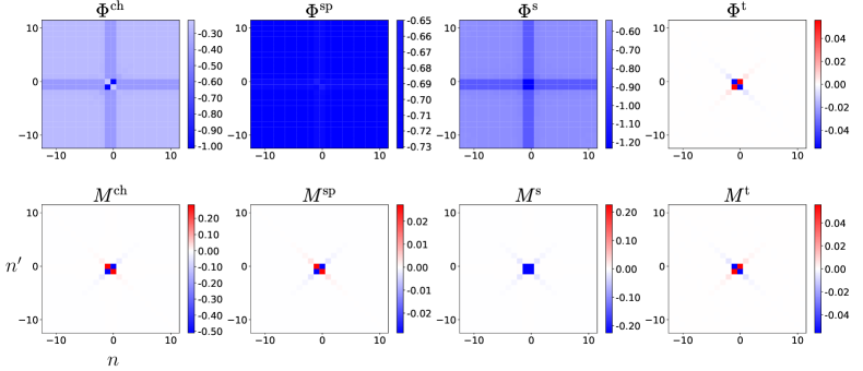
Figure 4: Reducible vertex functions of the atomic limit at $U/T=2$. Axes show the fermionic Matsubara indices ($\omega=0$). Top: $\Phi$ corresponding to the original parquet decomposition Eq. (6). Bottom: Vertices $M$ of the parquet expression Eq. (16).

Relation to Hedin’s equations:

The calculation scheme above differs from Hedin’s original work through the prescription for the ladder kernel $S$ in Step 3. In Hedin’s equations Onida et al. (2002); Held et al. (2011) the ladder kernel is given by the functional derivative $S=\delta(\Sigma-\Sigma^{H})/\delta G$ where $\Sigma^{H}=U\langle n\rangle/2$. With this $S$ and using $F-\Delta=T$ in Eq. (23a) the algorithm is equivalent to Hedin’s equations. This functional derivative is however difficult to calculate in practice. Here, instead, $S$ is obtained from the parquet diagrams in Step 3, as proved in Sec. IV.

VI Numerical examples

In this section we evaluate the key quantities that play a role in the efficient calculation scheme defined in Sec. V (e.g., $W,\gamma,M$) and demonstrate the low-energetic and short-ranged properties of the corresponding vertices $M$. As concrete examples we consider the exact solution of the atomic limit and the parquet approximation for the lattice Hubbard model at weak coupling.

Here, the results for the atomic limit have been obtained using the corresponding implementation made available with this paper Krien (2020); the relevant quantities for the Hubbard model have been evaluated using the victory implementation of the traditional parquet equations Li et al. (2019).

VI.1 Atomic Limit

We apply the BEPS method to a toy model, the atomic limit of e.g. the Hubbard model at half-filling. This model is exactly solvable and it has a nontrivial solution for the vertex functions. Analytical expressions for all components of the parquet decomposition Eq. (6) are available Thunström et al. (2018). Starting from the exact fully irreducible vertex $\Lambda_{\nu\nu^{\prime}\omega}$ the calculation cycle in Sec. V recovers the correlation functions of the atomic limit.

A Python implementation Krien (2020) is provided which converges on a single core within a few minutes .

We focus here on one advantage of the BEPS calculation scheme, evident already in the atomic limit, which is the decay of the vertex functions at high frequencies. The top panels of Fig. 4 show the reducible vertices $\Phi_{\nu\nu^{\prime}\omega}$ of the parquet decomposition in Eq. (6). The vertices belonging to the channels $\alpha=\text{ch},\text{sp},\text{s}$ have features that do not decay at high frequencies, whereas the triplet vertex $\alpha=\text{t}$ decays. This is the case because the bare interaction vanishes in the triplet channel, $U^{\text{t}}=0$. The bottom panels of Fig. 4 show the corresponding vertices $M_{\nu\nu^{\prime}\omega}$ of the parquet expression (16). Evidently, all features of these vertices decay at high frequency (in the case of the triplet channel trivially because $M^{\text{t}}=\Phi^{\text{t}}$).

VI.2 Parquet approximation

Next, we analyze the vertices in the parquet approximation for the weakly interacting Hubbard model on the square lattice at half-filling, $U/t=2$, where $t=1$ is the nearest neighbor hopping amplitude. The temperature is set to $T/t=0.2$. The lattice size is fixed to $8\times 8$ sites.

The victory implementation of the parquet method which we use here was presented in Ref. Li et al. (2019). It does not make use of the efficient calculation scheme presented in Sec. V, but it serves us to evaluate the vertices $F$ and $\Phi$ within the parquet approximation.

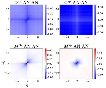
Figure 5: Reducible vertex functions in the parquet approximation, $U/t=2,T/t=0.2$. Fermionic momenta correspond to the antinode (AN), the bosonic momentum is set to $\mathbf{q}=(\pi,\pi)$, other labels as in Fig. 4.

As mentioned above, in the efficient calculation scheme the parquet approximation corresponds to setting the fully irreducible vertex in Eq. (16) to zero, $\tilde{\Lambda}^{\alpha}=0$, whereas the victory implementation actually evaluates Eq. (6) using $\Lambda^{\alpha}=\tilde{\Lambda}^{\alpha}+U^{\alpha}=U^{\alpha}$. We show in Appendix A how the vertices $M$ can be calculated from the converged solution for $F$ and $\Phi$. Their full momentum and frequency dependence is available to us,

$$M^{\text{ch}/\text{sp}}(\mathbf{k},\mathbf{k}^{\prime},\mathbf{q},\nu,\nu^{\prime},\omega).$$ (26)

First, we consider the asymptotic behavior of the vertices as a function of the frequencies. Fig. 5 shows the particle-hole vertices $\Phi^{\text{ch}/\text{sp}}$ and $M^{\text{ch}/\text{sp}}$, where we focus on the antinode, $\mathbf{k}=\mathbf{k}^{\prime}=\mathbf{k}_{\text{AN}}=(\pi,0)$, the bosonic momentum and frequency are set to $\mathbf{q}=(\pi,\pi)$ and $\omega=0$. This combination represents the scattering of particle and hole from the antinode to another antinode.

Similar to the atomic limit, the $M$’s decay as a function of $\nu,\nu^{\prime}$ in all directions, but their structure is more complicated due to the additional energy scale $t$.

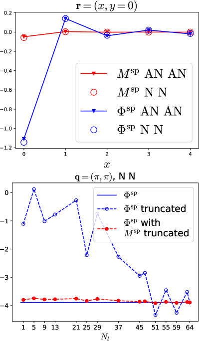
Figure 6: Top: Spatial dependence of $\Phi^{\text{sp}}$ and $M^{\text{sp}}$. The fermionic momenta correspond to the node or antinode. The alternating sign of $\Phi^{\text{sp}}$ indicates antiferromagnetic correlations. Bottom: Effect of truncation in the form-factor basis on the vertex $\Phi^{\text{sp}}$. Since $M^{\text{sp}}$ is much smaller than $\Phi^{\text{sp}}$ the form-factor truncation of $M^{\text{sp}}$ (red) is quantitatively superior to the direct truncation of $\Phi^{\text{sp}}$ (blue) [see text]. Results are for frequencies $\nu=\nu^{\prime}=\pi T$; $N_{\ell}=64$ corresponds to a calculation without truncation.

We note that in the current implementation it is not feasible to fully converge the Matsubara summations required for the calculation of the vertices $M$ (cf. Appendix A). The correspondence to the calculated $\Phi$ is therefore not perfect and $M^{\text{sp}}$ retains a small residual asymptote.

Next, we consider the spatial dependence of the vertices. To this end, we transform $\Phi^{\text{sp}}$ and $M^{\text{sp}}$ to real space with respect to the bosonic momentum, $\mathbf{q}\rightarrow\mathbf{r}$,

$$M^{\text{ch}/\text{sp}}(\mathbf{k},\mathbf{k}^{\prime},\mathbf{r},\nu,\nu^{\prime},\omega).$$ (27)

We fix the frequencies to $\nu=\nu^{\prime}=\pi T$, $\omega=0$. For the fermionic momenta we consider the antinode $\mathbf{k}=\mathbf{k}^{\prime}=\mathbf{k}_{\text{AN}}$ and the node $\mathbf{k}=\mathbf{k}^{\prime}=\mathbf{k}_{\text{N}}=(\frac{\pi}{2},\frac{\pi}{2})$.

The top panel of Fig. 6 shows $\Phi^{\text{sp}}$ and $M^{\text{sp}}$ as a function of $\mathbf{r}=(x,y=0)$ along the $x$-axis. Clearly visible is the alternating sign of $\Phi^{\text{sp}}$ characteristic of antiferromagnetic correlations. On the other hand, $M^{\text{sp}}$ is two orders of magnitude smaller than $\Phi^{\text{sp}}$. Similarly, in the charge channel $M^{\text{ch}}$ is much smaller than $\Phi^{\text{ch}}$ (not shown). Importantly, this fact alone implies that the spatial dependence of $\Phi=M+\Delta-U$ is largely determined by $\Delta$, the single-boson exchange Krien et al. (2020a). It explains the fast convergence of the truncated unity approximation Eckhardt et al. (2020) used in Refs. Krien et al. (2020a, b), where only the $M$’s were truncated in real space while the full spatial dependence of $\Delta$ was retained.

To underline this, we transform the vertex $\Phi^{\text{sp}}$ into the truncated unity (form-factor) basis Eckhardt et al. (2020) and back into $\mathbf{q}$-space, while discarding all but a number $N_{\ell}$ of basis functions (form factors) $f(\ell,\mathbf{q})$,

$$\Phi^{\text{sp}}(\mathbf{q},N_{\ell})\equiv\sum_{\ell=1}^{N_{\ell}}f^{*}(\ell,\mathbf{q})\sum_{\mathbf{q}^{\prime}}f(\ell,\mathbf{q}^{\prime})\Phi^{\text{sp}}(\mathbf{q}^{\prime}),$$ (28)

where we keep $\nu=\nu^{\prime}=\pi T,\omega=0,\mathbf{k}=\mathbf{k}^{\prime}=(\frac{\pi}{2},\frac{\pi}{2})$ fixed.

Obviously, $\Phi^{\text{sp}}(\mathbf{q},N_{\ell}=64)=\Phi^{\text{sp}}(\mathbf{q})$ recovers the complete momentum dependence, since there are as many form factors as there are lattice sites ($8\times 8$). Blue data points show the result for $\mathbf{q}=(\pi,\pi)$ in the bottom panel of Fig. 6, indicating a remarkably slow convergence of the expansion with the cutoff $N_{\ell}$ . Apparently, the antiferromagnetic correlations represented by $\Phi^{\text{sp}}$ should not be truncated in real space even at this high temperature.

To assess the advantage of the short-range nature of the vertex $M$ in the parquet equation with SBE decomposition [Eqs. (18a)-(18d)], we next apply the same procedure to the vertex $M^{\text{sp}}$. The red data points in the bottom panel of Fig. 6 show the resulting approximation for the thus determined $\Phi^{\text{sp}}(\mathbf{q})\approx M^{\text{sp}}(\mathbf{q},N_{\ell})+\Delta^{\text{sp}}(\mathbf{q})-U^{\text{sp}}$, which is reasonable even for $N_{\ell}=1$.

To interpret this result, it is important to remark that the relative error ${|M^{\text{sp}}(\mathbf{q})-M^{\text{sp}}(\mathbf{q},N_{\ell})|}/{|M^{\text{sp}}(\mathbf{q})|}$, for a given $\mathbf{q}$, can be similar to ${|\Phi^{\text{sp}}(\mathbf{q})-\Phi^{\text{sp}}(\mathbf{q},N_{\ell})|}/{|\Phi^{\text{sp}}(\mathbf{q})|}$. However, as is clear from the top panel of Fig. 6, the aim is to capture the coefficients $M^{\text{sp}}(\ell)=\sum_{\mathbf{q}}f(\ell,\mathbf{q})M^{\text{sp}}(\mathbf{q})$ which are significant relative to $\Phi^{\text{sp}}$. Therefore, it is sufficient to keep only a very small number of coefficients $M^{\text{sp}}(\ell)$, for example, the first form factor, $f(\ell=1,\mathbf{q})=1$, already captures the local component $\sum_{\mathbf{q}}M^{\text{sp}}(\mathbf{q})$ drawn in the top panel of Fig. 6 at $\mathbf{r}=(0,0)$.

We should also note that the $M^{\text{sp}}$ presented here was obtained in postprocessing and is not perfectly converged . Therefore, we can not determine the precise correlation content of this vertex, for example, whether it is completely free of antiferromagnetic correlations or instead captures some of them. In the future, the implementation of the efficient calculation scheme presented in Sec. V may ultimatively clarify this, because it allows for determining $M$ with the same accuracy as $\Phi$.

Finally, let us estimate the numerical scaling of the newly proposed scheme as compared to the traditional parquet implementation. For a frequency box of linear size $N_{\omega}$ and $N_{q}$ momentum points in the Brillouin zone, the standard parquet calculation requires virtual memory that scales with $\mathcal{O}(N_{q}^{3}{N}_{\omega}^{3})$ and the computational effort scales with $\mathcal{O}(N_{q}^{4}{N}_{\omega}^{4})$ for the Bethe-Salpeter equation (13) and with $\mathcal{O}(N_{q}^{3}{N}_{\omega}^{3})$ for the parquet equation (6). In practice, however, large vertices $\Phi$ need to be stored in distributed memory and internodal communication and memory access operations needed in evaluating Eq. (6) are the actual bottleneck.

In the scheme proposed here the $M$ vertices need only a much smaller frequency box $\widetilde{N}_{\omega}$. The actual memory requirement $\mathcal{O}(N_{q}^{3}\widetilde{N}_{\omega}^{3})$ is thus reduced. Additionally, we need to store three-leg vertices $\gamma$ which scale like $\mathcal{O}(N_{q}^{2}\widetilde{N}_{\omega}^{2})$. Using the form-factor basis to represent the momentum dependence of $M$, this scaling is further reduced to $\mathcal{O}(N_{\ell}^{3}\widetilde{N}_{\omega}^{3})$ for the $M$’s. With just few (or even only one as Fig. 6 demonstrates) form factors and small $\widetilde{N}_{\omega}$, the dominant part is the quadratic scaling in $N_{q}\widetilde{N}_{\omega}$ for $\gamma$’s. The computational effort of the new Bethe-Salpeter equation [Step 4, Eqs. (22a)-(22b)] scales then with $\mathcal{O}(N_{\ell}^{4}\widetilde{N}_{\omega}^{4})$ and the parquet equations in form-factor basis [Step 3, Eqs. (18a)-(18d)] with $\mathcal{O}(N_{\ell}^{6}\widetilde{N}_{\omega}^{3}$). Due to significantly smaller vertices $M$ and $\gamma$, the memory access bottleneck can be removed (the $\Delta$’s do not need to be stored) .

VI.3 Comparison to $GW$ approximation

We now draw a connection between the parquet and $GW$ approximations, paying special attention to the role of vertex corrections. To this end, we recall Eq. (24) for the parquet self-energy, which is drawn as a diagram at the bottom of Fig. 7.

Let us examine the effect of dropping the vertex corrections in different places. The most straightforward way to do this is to set $\gamma=1$ only in the defining equation for $\Sigma$, which is then given as

$$\Sigma^{GW}_{k}-\Sigma^{H}=-\frac{1}{2}\sum_{q}G_{k+q}\left[W^{\text{ch}}_{q}+W^{\text{sp}}_{q}\right],$$ (29)

where $G$ and $W$ are the Green’s function and the screened interaction corresponding to the parquet approximation. The thus defined $\Sigma^{GW}$ is shown in Fig. 8 (cyan) next to the complete parquet self-energy (red), where $U/t=2,T/t=0.2$, as before. Apparently, for these parameters the direct contribution of vertex corrections to the self-energy is not very large and thus $\Sigma^{GW}$ is still a reasonable approximation. The inset of Fig. 8 shows that $\gamma^{\text{ch}}$ and $\gamma^{\text{sp}}$ deviate from their noninteracting value $1$ by roughly up to 30% and 15%, respectively. The bottom panel of Fig. 9 shows that $\gamma^{\text{ch}/\text{sp}}$ are suppressed mainly around the bosonic momentum $\mathbf{q}=(\pi,\pi)$.

Figure 7: Hedin’s equations for the polarization (top) and the self-energy (bottom). Neglecting vertex corrections corresponds to setting $\gamma=1$.

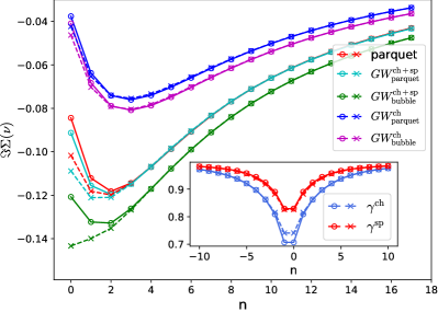
Figure 8: Imaginary part of the self-energy comparing the parquet approximation (red) with various $GW$-like approximations (see text; purple: actual $GW$ approximation) for the half-filled square lattice Hubbard model at $U/t=2,T/t=0.2$ as a function of the Matsubara index. Two momenta are shown, corresponding to the node (empty circles) and antinode (crosses). Inset: Hedin vertex $\gamma^{\text{ch}}$ (blue) and $\gamma^{\text{sp}}$ (red) as a function of the fermionic frequency. Fermionic momenta correspond to the node (empty circles) or antinode (crosses) and the bosonic momentum and frequency are set to ${\bf q}=(\pi,\pi)$ and $\omega=0$.

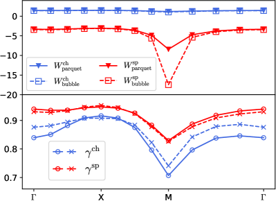
Figure 9: Top: Screened interaction in the parquet approximation (full lines) and neglecting vertex corrections [cf. Eq. (30)] (dashed lines) as a function of $\mathbf{q}$. Bottom: Hedin vertex $\gamma^{\text{ch}}$ (blue) and $\gamma^{\text{sp}}$ (red). The fermionic momentum $\mathbf{k}$ corresponds to the node (empty circles) or antinode (crosses); $\nu=\pi T,\omega=0$. Parameters as in Fig. 8.

One needs to keep in mind, however, that the vertex corrections appear in all diagrammatic objects drawn in Fig. 7 (i.e., $G,W,\gamma$). Therefore, to approach a $GW$-like approximation of any practical value, we need to drop further vertex corrections. For example, let us recall that the screened interaction defined in Eq. (20a) incorporates vertex corrections via the polarization, which is drawn as a diagram on the top of Fig. 7. Consequently, for an actual $GW$ calculation one should use here only a bubble of parquet Green’s functions for $\Pi$,

$$\Pi^{GW}_{q}=\sum_{k}G_{k}G_{k+q}.$$ (30)

The resulting screened interactions (dashed lines) are drawn in the top panel of Fig. 9 in comparison to the parquet approximation (full lines). While $W^{\text{ch}}$ is similar to the parquet result (but anyways almost momentum independent), the large difference for $W^{\text{sp}}$ reveals the significant screening facilitated by $\gamma^{\text{sp}}$.

If we use the bubble back in Eq. (29), the (absolutely) much larger $W^{\text{sp}}$ in the bubble approximation for the screening leads to a huge feedback on the self-energy: Fig. 8 (green) shows even an insulating-like behavior at the antinodal point, far above the temperature where this is expected to happen Schäfer et al. (2020); Krien et al. (2020b).

The $15\%$-suppression of $\gamma^{\text{sp}}$ shown in the inset of Fig. 8 therefore crucially determines the Stoner enhancement $(1-U^{\text{sp}}\Pi^{\text{sp}})^{-1}$ in the proximity of the spin-density wave. This suppression is the result of the particle-particle vertex correction  considered by Kanamori Kanamori (1963). To arrive at a reasonable approximation for $W^{\text{sp}}$ this effect needs to be taken into account in some way, for example, by replacing $U^{\text{sp}}$ with an effective interaction, which is the essence of the two-particle self-consistent approach Y.M. Vilk and A.-M.S. Tremblay (1997) and of the Moriya-$\lambda$ correction Moriya (1985); Katanin et al. (2009).

Finally, we note that in this work we employed the Fierz ratio $\frac{1}{2}$ for the self-energy in Eq. (24), which corresponds to a symmetric splitting between the charge and spin channels. This is a natural choice because it leads to a cancellation of slowly decaying Matsubara summations Krien and Valli (2019) in Eq. (24).

Usually, however, in $GW$ the self-energy is expressed only through $W^{\text{ch}}$ (and $\gamma^{\text{ch}}$) Hedin (1965), which, at first glance, seems useful to avoid problems due to the instability in the spin channel. However, Fig. 8 shows that the corresponding result for the self-energy using only $W^{\text{ch}}$ from the parquet calculation (dark blue) is significantly worse than the symmetric approximation (cyan) in Eq. (29), confirming that for an optimal result the channels should be mixed Ayral et al. (2017); Schäfer and Toschi (2020). Also, using the noninteracting Green’s function $G^{0}$ to calculate $\Pi^{GW}$ and $\Sigma^{GW}$ is even worse, as $W^{\text{sp}}$ is then already outside of its convergence radius for these parameters (not shown). We should note that the decoupling ambiguity is a peculiarity of the Hubbard interaction $Un_{\uparrow}n_{\downarrow}$. It does not affect nonlocal interactions between charge or spin densities.

VII Discussion and Conclusions

The parquet equations for real fermions were reformulated into a computationally more feasible form by combining them with Hedin’s $GW\gamma$ formalism. From the viewpoint of the latter our approach yields the parquet diagrams for $\gamma$ in terms of single- and multi-boson exchange. This offers a new perspective on vertex corrections in electronic systems. For example, the association of certain vertex diagrams with effective particles becomes very explicit Kauch et al. (2020), or the notion of a ‘bosonic glue’ that may play a role for phenomena such as high temperature superconductivity Kitatani et al. (2019) can be taken more literally.

The resulting calculation scheme, which was coined a boson exchange parquet solver (BEPS) in Ref. Krien et al. (2020a), has no disadvantages in comparison to previous implementations of the parquet equations but offers two strong advantages. Namely, the vertex asymptotics and, in the case of a lattice system Krien et al. (2020a), also the long-ranged fluctuations are removed from the parquet equations through their exact reformulation.

This goes beyond the asymptotic treatment of the vertices pioneered in Refs. Kuneš (2011); Li et al. (2016); Wentzell et al. (2020) which improves the feasibility of parquet solvers Li et al. (2016); Tagliavini et al. (2018); Kaufmann (2017), but the low-energy aspect of the single-boson exchange remains intermixed with all other fluctuations. Instead, the BEPS method corresponds to a kind of separation of the fluctuations that is exact also at low frequencies Krien (2019); Katanin (2020). In Ref. Krien et al. (2020a) and here this idea was adopted to the parquet formalism for dual fermions and real fermions, respectively. Let us stress that BEPS for real fermions is an exact unification of Hedin’s equations and the parquet equations. An approximation only enters when the fully irreducible vertex $\Lambda$ is replaced by an approximated one such as the bare interaction $U$ in the parquet approximation or all local diagrams in the D$\Gamma$A, Toschi et al. (2007); Valli et al. (2015); Li et al. (2016, 2019); Ayral and Parcollet (2016) . In this respect our approach does not differ from the traditional parquet method, that is, it does not introduce any additional approximations.

As numerical results we first discussed the simple case of a quantum impurity model, where the spatial degrees of freedom do not play a role. The computational efficiency of the calculation scheme is then improved through the decay properties of the vertices. Remarkably, this is sufficient to solve the parquet equations for the atomic limit on a laptop using the provided Python script Krien (2020).

We also analyzed the parquet approximation for the lattice Hubbard model using the victory code presented in Ref. Li et al. (2019). We evaluated the vertices that correspond to the BEPS method and verified that they indeed exhibit the useful decay properties. This underlines the accuracy of the asymptotic treatment of the vertices in this implementation Li et al. (2016). We discussed $GW$-like approximations for the self-energy, highlighting the crucial importance of vertex corrections represented by the Hedin vertex $\gamma$, which even increases at low temperature Krien et al. (2020b). However, we find it plausible that neglecting vertex corrections has a less severe effect away from particle-hole symmetry and in dimensions $>\!2$. With respect to recent works investigating the feedback of spin fluctuations on the optical conductivity Kauch et al. (2020); Worm et al. (2020); Simard et al. (2020), it is intriguing to consider the role of the fermion-boson coupling also in this context.

In the future we will implement the efficient calculation scheme into the victory code Li et al. (2019). This seems promising because in Refs. Krien et al. (2020a, b), which discussed the lattice case for dual fermions, it is shown that the BEPS method unfolds its full power in combination with the truncated unity (TU) approximation Husemann and Salmhofer (2009); Wang et al. (2012); Platt et al. (2013); Lichtenstein et al. (2017); Eckhardt et al. (2020), which corresponds to a real space truncation of the vertices. We expect (cf. Fig. 6) also for real fermions a similar improved convergence with the form factors compared to the truncated unity parquet solver (TUPS, Eckhardt et al. (2020)). While the form factors correspond to a suitable basis for the spatial degrees of freedom, the computational efficiency may be further improved by introducing an optimal basis for the frequencies Shinaoka et al. (2018); Witt et al. (2020); Wallerberger et al. (2020). Such a treatment should pave the way for parquet calculations including at least a few orbitals such as the two $e_{g}$- or three $t_{2g}$-orbitals of a transition metal oxide, or the $J=5/2$ multiplet of an $f$-electron system.

Lastly, some words are in place regarding the closely related method for dual fermions presented in Ref. Krien et al. (2020a): Diagrammatically, both approaches are the same, but the basic building blocks are different. In Ref. Krien et al. (2020a) the (real fermion) Green’s function lines are replaced by dual fermion lines and the equations defining the self-energy, polarization, and Hedin vertex assume a different form. In the present paper, the starting point is an approximation for the two-particle fully irreducible vertex $\Lambda$. In contrast, in the dual fermion formulation Krien et al. (2020a) local reducible interactions are included, hence using, e.g., a local full vertex $F_{\text{loc}}$ for dual fermions instead of a local $\Lambda_{\text{loc}}$ in D$\Gamma$A. This leads to an interesting distinction between the bosonization of the parquet equations for real and dual fermions, respectively, which corresponds to removing the interaction-reducible diagrams from either $F_{\text{loc}}$ or $\Lambda_{\text{loc}}$: In the case of real fermions $\Lambda_{\text{loc}}$ includes only one such diagram, the bare interaction itself, whereas for dual fermions $F_{\text{loc}}$ contains many interaction-reducible diagrams which need to be separated off using the (local) SBE decomposition Krien et al. (2019).

The approaches for real and dual fermions both have their pros and cons. The parquet solver discussed in the present paper is simpler, an integral part of many different approaches, the interpretation in terms of real fermions is easier, and the approximation made for $\Lambda$ is very explicit. On the other hand, the connecting dual fermion lines decay much faster, which, in combination with the decay of the vertex functions facilitated by the BEPS method, leads to a very high computational efficiency of the dual parquet solver Krien et al. (2020a). Further, the dual fermions are not affected by divergences of the vertex $\Lambda_{\text{loc}}$ Schäfer et al. (2013). It is noteworthy that, due to the dependence of the bare dual fermion interaction ($F_{\text{loc}}$) on three frequencies, the (parquet) dual self-energy can not be expressed in terms of $G,W$, and $\gamma$ alone Krien et al. (2020b). This is possible for the real fermion representation, which allowed us here to to establish a connection between the parquet and $GW\gamma$ methods.

Appendix A Evaluation of vertices $M$

Here, we show how the vertices $M^{\alpha}$ in the parquet expression (16) can be calculated from a converged result of the victory code Li et al. (2019), that is, the Green’s function $G$ and the vertices $\Phi$ and $F$ in the parquet decomposition (6) are known. We focus on the particle-hole channels $\alpha=\text{ch},\text{sp}$. First, we determine the susceptibility and the screened interaction,

$$X^{\alpha}_{q}= 2\sum_{k}G_{k}G_{k+q}+2\sum_{kk^{\prime}q}G_{k}G_{k+q}F^{\alpha}_{kk^{\prime}q}G_{k^{\prime}}G_{k^{\prime}+q},$$

$$W^{\alpha}_{q}=U^{\alpha}\left(1+\frac{1}{2}X^{\alpha}_{q}U^{\alpha}\right).$$ (31)

Next, we evaluate the Hedin vertex $\gamma$. We insert Eq. (4) into Eq. (5a),

$$\gamma^{\alpha}_{kq}= 1+\sum_{k^{\prime}}(F^{\alpha}_{kk^{\prime}q}-\gamma^{\alpha}_{kq}W^{\alpha}_{q}\gamma^{\alpha}_{k^{\prime}q})G_{k^{\prime}}G_{k^{\prime}+q}$$

$$= 1+\sum_{k^{\prime}}F^{\alpha}_{kk^{\prime}q}G_{k^{\prime}}G_{k^{\prime}+q}-\gamma^{\alpha}_{kq}W^{\alpha}_{q}\Pi^{\alpha}_{q}$$

$$= 1+\sum_{k^{\prime}}F^{\alpha}_{kk^{\prime}q}G_{k^{\prime}}G_{k^{\prime}+q}-\gamma^{\alpha}_{kq}\frac{1}{2}U^{\alpha}X^{\alpha}_{q}.$$ (32)

From the first to the second line we identified the polarization $\Pi$ using Eq. (3). From the second to the third line we used Eq. (2) and $X^{\alpha}_{q}=2\Pi^{\alpha}_{q}/(1-U^{\alpha}\Pi^{\alpha}_{q})$. We solve Eq. (32) for $\gamma$,

$$\gamma^{\alpha}_{kq}= \frac{1+\sum_{k^{\prime}}F^{\alpha}_{kk^{\prime}q}G_{k^{\prime}}G_{k^{\prime}+q}}{W^{\alpha}_{q}/U^{\alpha}},$$ (33)

where we used again Eq. (31). With $\gamma$ and $W$ we finally obtain $M$ from Eq. (14) (see also Fig. 2),

$${M}^{\alpha}_{kk^{\prime}q}=\Phi^{\alpha}_{kk^{\prime}q}-\gamma^{\alpha}_{kq}W^{\alpha}_{q}\gamma^{\alpha}_{k^{\prime}q}+U^{\alpha}.$$ (34)

We do not evaluate $M^{\text{s}/\text{t}}$ in the particle-particle channel. However, for the singlet channel $\alpha=\text{s}$ the steps are analogous, starting from Eq. (5b) and taking into account the factor $\frac{1}{2}$. For the triplet channel nothing needs to be done since $M^{\text{t}}=\Phi^{\text{t}}$.

References

- De Dominicis and Martin (1964a) Cyrano De Dominicis and Paul C. Martin, “Stationary Entropy Principle and Renormalization in Normal and Superfluid Systems. II. Diagrammatic Formulation,” Journal of Mathematical Physics 5, 31–59 (1964a).
- Diatlov et al. (1957) I. T. Diatlov, V. V. Sudakov, and K. A. Ter-Martirosian, “Asymptotic meson-meson scattering theory,” Soviet Phys. JETP 5, 631 (1957).
- Hedin (1965) Lars Hedin, “New Method for Calculating the One-Particle Green’s Function with Application to the Electron-Gas Problem,” Phys. Rev. 139, A796–A823 (1965).
- Bickers (2004) N. E. Bickers, “Self-Consistent Many-Body Theory for Condensed Matter Systems,” in Theoretical Methods for Strongly Correlated Electrons, edited by David Sénéchal, André-Marie Tremblay, and Claude Bourbonnais (Springer New York, New York, NY, 2004) pp. 237–296.
- Tam et al. (2013) Ka-Ming Tam, H. Fotso, S.-X. Yang, Tae-Woo Lee, J. Moreno, J. Ramanujam, and M. Jarrell, “Solving the parquet equations for the Hubbard model beyond weak coupling,” Phys. Rev. E 87, 013311 (2013).
- Rohringer et al. (2012) G. Rohringer, A. Valli, and A. Toschi, “Local electronic correlation at the two-particle level,” Phys. Rev. B 86, 125114 (2012).
- Valli et al. (2015) A. Valli, T. Schäfer, P. Thunström, G. Rohringer, S. Andergassen, G. Sangiovanni, K. Held, and A. Toschi, “Dynamical vertex approximation in its parquet implementation: Application to Hubbard nanorings,” Phys. Rev. B 91, 115115 (2015).
- Li et al. (2016) Gang Li, Nils Wentzell, Petra Pudleiner, Patrik Thunström, and Karsten Held, “Efficient implementation of the parquet equations: Role of the reducible vertex function and its kernel approximation,” Phys. Rev. B 93, 165103 (2016).
- Li et al. (2019) Gang Li, Anna Kauch, Petra Pudleiner, and Karsten Held, “The victory project v1.0: An efficient parquet equations solver,” Comput. Phys. Commun 241, 146 – 154 (2019).
- Astretsov et al. (2020) Grigory V. Astretsov, Georg Rohringer, and Alexey N. Rubtsov, “Dual parquet scheme for the two-dimensional Hubbard model: Modeling low-energy physics of high- cuprates with high momentum resolution,” Phys. Rev. B 101, 075109 (2020).
- Friederich et al. (2011) S. Friederich, H. C. Krahl, and C. Wetterich, “Functional renormalization for spontaneous symmetry breaking in the Hubbard model,” Phys. Rev. B 83, 155125 (2011).
- Metzner et al. (2012) Walter Metzner, Manfred Salmhofer, Carsten Honerkamp, Volker Meden, and Kurt Schönhammer, “Functional renormalization group approach to correlated fermion systems,” Rev. Mod. Phys. 84, 299–352 (2012).
- Tagliavini et al. (2019) Agnese Tagliavini, Cornelia Hille, Fabian B. Kugler, Sabine Andergassen, Alessandro Toschi, and Carsten Honerkamp, “Multiloop functional renormalization group for the two-dimensional Hubbard model: Loop convergence of the response functions,” SciPost Phys. 6, 9 (2019).
- Kauch et al. (2019) Anna Kauch, Felix Hörbinger, Gang Li, and Karsten Held, “Interplay between magnetic and superconducting fluctuations in the doped 2d Hubbard model,” (2019), arXiv:1901.09743 .
- Pudleiner et al. (2019) Petra Pudleiner, Anna Kauch, Karsten Held, and Gang Li, “Competition between antiferromagnetic and charge density wave fluctuations in the extended Hubbard model,” Phys. Rev. B 100, 075108 (2019).
- Onida et al. (2002) Giovanni Onida, Lucia Reining, and Angel Rubio, “Electronic excitations: density-functional versus many-body Green’s-function approaches,” Rev. Mod. Phys. 74, 601–659 (2002).
- Held et al. (2011) K. Held, C. Taranto, G. Rohringer, and A. Toschi, “Hedin Equations, , +DMFT, and All That,” (2011), arXiv:1109.3972 .
- Toschi et al. (2007) A. Toschi, A. A. Katanin, and K. Held, “Dynamical vertex approximation: A step beyond dynamical mean-field theory,” Phys. Rev. B 75, 045118 (2007).
- Katanin et al. (2009) A. A. Katanin, A. Toschi, and K. Held, “Comparing pertinent effects of antiferromagnetic fluctuations in the two- and three-dimensional Hubbard model,” Phys. Rev. B 80, 075104 (2009).
- Rohringer et al. (2018) G. Rohringer, H. Hafermann, A. Toschi, A. A. Katanin, A. E. Antipov, M. I. Katsnelson, A. I. Lichtenstein, A. N. Rubtsov, and K. Held, “Diagrammatic routes to nonlocal correlations beyond dynamical mean field theory,” Rev. Mod. Phys. 90, 025003 (2018).
- Godby et al. (1988) R. W. Godby, M. Schlüter, and L. J. Sham, “Self-energy operators and exchange-correlation potentials in semiconductors,” Phys. Rev. B 37, 10159–10175 (1988).
- Aryasetiawan and Gunnarsson (1998) F Aryasetiawan and O Gunnarsson, “The method,” Reports on Progress in Physics 61, 237–312 (1998).
- Biermann et al. (2003) S. Biermann, F. Aryasetiawan, and A. Georges, “First-Principles Approach to the Electronic Structure of Strongly Correlated Systems: Combining the Approximation and Dynamical Mean-Field Theory,” Phys. Rev. Lett. 90, 086402 (2003).
- Tomczak et al. (2017) J. M. Tomczak, P. Liu, A. Toschi, G. Kresse, and K. Held, “Merging with DMFT and non-local correlations beyond,” The European Physical Journal Special Topics 226, 2565–2590 (2017).
- Nilsson et al. (2017) F. Nilsson, L. Boehnke, P. Werner, and F. Aryasetiawan, “Multitier self-consistent ,” Phys. Rev. Materials 1, 043803 (2017).
- Maggio and Kresse (2017) E. Maggio and G. Kresse, “ Vertex Corrected Calculations for Molecular Systems,” J. Chem. Theory Comput. 13, 4765 (2017).
- Smith (1992) Roger Alan Smith, “Planar version of Baym-Kadanoff theory,” Phys. Rev. A 46, 4586–4597 (1992).
- Janiš (1999) V. Janiš, “Stability of self-consistent solutions for the Hubbard model at intermediate and strong coupling,” Phys. Rev. B 60, 11345–11360 (1999).
- Janiš and Kolorenč (2005) V. Janiš and J. Kolorenč, “Mean-field theories for disordered electrons: Diffusion pole and Anderson localization,” Phys. Rev. B 71, 245106 (2005).
- Janiš et al. (2017) Václav Janiš, Anna Kauch, and Vladislav Pokorný, “Thermodynamically consistent description of criticality in models of correlated electrons,” Phys. Rev. B 95, 045108 (2017).
- Kugler and von Delft (2018) Fabian B Kugler and Jan von Delft, “Derivation of exact flow equations from the self-consistent parquet relations,” New Journal of Physics 20, 123029 (2018).
- Krien (2018) Friedrich Krien, Conserving dynamical mean-field approaches to strongly correlated systems, PhD Thesis (Hamburg, 2018).
- Almbladh et al. (1999) C.-O. Almbladh, U. von Barth, and R. van Leeuwen, “Variational total energies from - and -derivable theories,” International Journal of Modern Physics B 13, 535–541 (1999).
- Chubukov and Wölfle (2014) Andrey V. Chubukov and Peter Wölfle, “Quasiparticle interaction function in a two-dimensional Fermi liquid near an antiferromagnetic critical point,” Phys. Rev. B 89, 045108 (2014).
- (35) A. I. Larkin and A. A. Varlamov, “Fluctuation Phenomena in Superconductors,” in Superconductivity (Springer Berlin Heidelberg) pp. 369–458.
- Aslamasov and Larkin (1968) L.G. Aslamasov and A.I. Larkin, “The influence of fluctuation pairing of electrons on the conductivity of normal metal,” Physics Letters A 26, 238 – 239 (1968).
- Bergeron et al. (2011) Dominic Bergeron, Vasyl Hankevych, Bumsoo Kyung, and A. M. S. Tremblay, “Optical and dc conductivity of the two-dimensional Hubbard model in the pseudogap regime and across the antiferromagnetic quantum critical point including vertex corrections,” Phys. Rev. B 84, 085128 (2011).
- Krien et al. (2019) Friedrich Krien, Angelo Valli, and Massimo Capone, “Single-boson exchange decomposition of the vertex function,” Phys. Rev. B 100, 155149 (2019).
- Krien et al. (2020a) Friedrich Krien, Angelo Valli, Patrick Chalupa, Massimo Capone, Alexander I. Lichtenstein, and Alessandro Toschi, “Boson-exchange parquet solver for dual fermions,” Phys. Rev. B 102, 195131 (2020a).
- Rubtsov et al. (2008) A. N. Rubtsov, M. I. Katsnelson, and A. I. Lichtenstein, “Dual fermion approach to nonlocal correlations in the Hubbard model,” Phys. Rev. B 77, 033101 (2008).
- Krien et al. (2020b) Friedrich Krien, Alexander I. Lichtenstein, and Georg Rohringer, “Fluctuation diagnostic of the nodal/antinodal dichotomy in the Hubbard model at weak coupling: A parquet dual fermion approach,” Phys. Rev. B 102, 235133 (2020b).
- Krien (2020) Friedrich Krien, “Boson Exchange Parquet Solver,” https://github.com/fkrien/beps (2020).
- Wentzell et al. (2020) Nils Wentzell, Gang Li, Agnese Tagliavini, Ciro Taranto, Georg Rohringer, Karsten Held, Alessandro Toschi, and Sabine Andergassen, “High-frequency asymptotics of the vertex function: Diagrammatic parametrization and algorithmic implementation,” Phys. Rev. B 102, 085106 (2020).
- Note (1) We use a Fierz splitting of between charge and spin channels Krien and Valli (2019).
- Del Sole et al. (1994) R. Del Sole, Lucia Reining, and R. W. Godby, “ approximation for electron self-energies in semiconductors and insulators,” Phys. Rev. B 49, 8024–8028 (1994).
-
Note (2)
Due to this interaction-irreducible property of the Hedin vertex it satisfies the ladder
equations Hedin (1965),
where is the corresponding Bethe-Salpeter kernel without the bare interaction, defined in Eq. (12\@@italiccorr). - De Dominicis and Martin (1964b) Cyrano De Dominicis and Paul C. Martin, “Stationary Entropy Principle and Renormalization in Normal and Superfluid Systems. I. Algebraic Formulation,” Journal of Mathematical Physics 5, 14–30 (1964b).
- Gunnarsson et al. (2016) O. Gunnarsson, T. Schäfer, J. P. F. LeBlanc, J. Merino, G. Sangiovanni, G. Rohringer, and A. Toschi, “Parquet decomposition calculations of the electronic self-energy,” Phys. Rev. B 93, 245102 (2016).
- Note (3) One may also say that the vertices are reducible with respect to the screened interaction , however, it is useful to consider also the bare interaction diagram as reducible Krien et al. (2019). Interestingly, the bare interaction does not play a role after we have passed over to the parquet expression Eq. (16\@@italiccorr), which implies that -reducibility is a meaningful concept after the bosonization. Indeed, in a functional formulation of the approach the screened interaction plays the role of a fundamental variable Almbladh et al. (1999).
- Note (4) Compare also Figs. 3 and 4 in Ref. Krien et al. (2019). In other words, interaction reducibility implies two-particle reducibility, with the only exception of the bare interaction itself, which is (fully) two-particle irreducible.
- Rohringer and Toschi (2016) G. Rohringer and A. Toschi, “Impact of nonlocal correlations over different energy scales: A dynamical vertex approximation study,” Phys. Rev. B 94, 125144 (2016).
- Sun and Kotliar (2002) Ping Sun and Gabriel Kotliar, “Extended dynamical mean-field theory and method,” Phys. Rev. B 66, 085120 (2002).
- Thunström et al. (2018) P. Thunström, O. Gunnarsson, Sergio Ciuchi, and G. Rohringer, “Analytical investigation of singularities in two-particle irreducible vertex functions of the Hubbard atom,” Phys. Rev. B 98, 235107 (2018).
- Note (5) Due to the exponential difference between charge and spin fluctuations in the atomic limit the linear mixing used in the provided script does not work for large values of . A nonlinear root-finder improves the convergence Krien and Valli (2019).
- Eckhardt et al. (2020) Christian J. Eckhardt, Carsten Honerkamp, Karsten Held, and Anna Kauch, “Truncated unity parquet solver,” Phys. Rev. B 101, 155104 (2020).
- Note (6) The truncated unity approximation applied to fermionic momentum dependence of converges much faster in . This fact was already largely explored in Ref. \rev@citealpEckhardt20. By evaluating the parquet equation [Eq. (6\@@italiccorr)] one however effectively approximates also the bosonic momentum (see Ref. \rev@citealpEckhardt20 for a detailed discussion).
- Note (7) The original victory implementation does not use , or vertices as an inherent part of the computation and therefore it is not optimized to obtain them with the same accuracy as . As a consequence, e.g., the tails of and the tails of are not treated equally (within the code or in postprocessing, respectively).
- Note (8) The advantage of this scheme in comparison with the TUPS implementation of Ref. Eckhardt et al. (2020), which also uses form-factors, is twofold: (i) we can use significantly fewer form factors and also transform the bosonic momentum; (ii) the frequency box can be chosen smaller.
- Schäfer et al. (2020) Thomas Schäfer, Nils Wentzell, Fedor Šimkovic IV, Yuan-Yao He, Cornelia Hille, Marcel Klett, Christian J. Eckhardt, Behnam Arzhang, Viktor Harkov, François-Marie Le Régent, Alfred Kirsch, Yan Wang, Aaram J. Kim, Evgeny Kozik, Evgeny A. Stepanov, Anna Kauch, Sabine Andergassen, Philipp Hansmann, Daniel Rohe, Yuri M. Vilk, James P. F. LeBlanc, Shiwei Zhang, A. M. S. Tremblay, Michel Ferrero, Olivier Parcollet, and Antoine Georges, “Tracking the Footprints of Spin Fluctuations: A Multi-Method, Multi-Messenger Study of the Two-Dimensional Hubbard Model,” (2020), arXiv:2006.10769 [cond-mat.str-el] .
- Note (9) See Refs. Kitatani et al. (2019); Krien et al. (2020a) for a calculation of the particle-particle vertex correction in the Anderson impurity model.
- Kanamori (1963) Junjiro Kanamori, “Electron correlation and ferromagnetism of transition metals,” Prog. Theor. Phys. 30, 275–289 (1963).
- Y.M. Vilk and A.-M.S. Tremblay (1997) Y.M. Vilk and A.-M.S. Tremblay, “Non-Perturbative Many-Body Approach to the Hubbard Model and Single-Particle Pseudogap,” J. Phys. I France 7, 1309–1368 (1997).
- Moriya (1985) Toru Moriya, Spin fluctuations in itinerant electron magnetism, Vol. 56 (Springer-Verlag Berlin, 1985).
- Krien and Valli (2019) Friedrich Krien and Angelo Valli, “Parquetlike equations for the Hedin three-leg vertex,” Phys. Rev. B 100, 245147 (2019).
- Ayral et al. (2017) Thomas Ayral, Jaksa Vučičević, and Olivier Parcollet, “Fierz Convergence Criterion: A Controlled Approach to Strongly Interacting Systems with Small Embedded Clusters,” Phys. Rev. Lett. 119, 166401 (2017).
- Schäfer and Toschi (2020) T. Schäfer and A. Toschi, “How to read between the lines of electronic spectra: the diagnostics of fluctuations in strongly correlated electron systems,” (2020), arXiv:2012.03604 .
- Kauch et al. (2020) A. Kauch, P. Pudleiner, K. Astleithner, P. Thunström, T. Ribic, and K. Held, “Generic Optical Excitations of Correlated Systems: -tons,” Phys. Rev. Lett. 124, 047401 (2020).
- Kitatani et al. (2019) Motoharu Kitatani, Thomas Schäfer, Hideo Aoki, and Karsten Held, “Why the critical temperature of high- cuprate superconductors is so low: The importance of the dynamical vertex structure,” Phys. Rev. B 99, 041115(R) (2019).
- Kuneš (2011) Jan Kuneš, “Efficient treatment of two-particle vertices in dynamical mean-field theory,” Phys. Rev. B 83, 085102 (2011).
- Tagliavini et al. (2018) Agnese Tagliavini, Stefan Hummel, Nils Wentzell, Sabine Andergassen, Alessandro Toschi, and Georg Rohringer, “Efficient Bethe-Salpeter equation treatment in dynamical mean-field theory,” Phys. Rev. B 97, 235140 (2018).
- Kaufmann (2017) J. Kaufmann, Calculation of Vertex Asymptotics from Local Correlation Functions, Master Thesis, TU Wien (2017).
- Krien (2019) Friedrich Krien, “Efficient evaluation of the polarization function in dynamical mean-field theory,” Phys. Rev. B 99, 235106 (2019).
- Katanin (2020) A. Katanin, “Improved treatment of fermion-boson vertices and Bethe-Salpeter equations in nonlocal extensions of dynamical mean field theory,” Phys. Rev. B 101, 035110 (2020).
- Ayral and Parcollet (2016) Thomas Ayral and Olivier Parcollet, “Mott physics and collective modes: An atomic approximation of the four-particle irreducible functional,” Phys. Rev. B 94, 075159 (2016).
- Note (10) This statement holds notwithstanding cutoff and truncation errors, e.g., of Matsubara summations, in a particular implementation.
- Worm et al. (2020) Paul Worm, Clemens Watzenböck, Matthias Pickem, Anna Kauch, and Karsten Held, “Broadening and sharpening of the Drude peak through antiferromagnetic fluctuations,” (2020), arXiv:2010.15797 .
- Simard et al. (2020) Olivier Simard, Shintaro Takayoshi, and Philipp Werner, “Diagrammatic study of optical excitations in correlated systems,” (2020), arXiv:2010.09052 .
- Husemann and Salmhofer (2009) C. Husemann and M. Salmhofer, “Efficient parametrization of the vertex function, scheme, and the Hubbard model at van Hove filling,” Phys. Rev. B 79, 195125 (2009).
- Wang et al. (2012) Xin Wang, M. J. Han, Luca de’ Medici, Hyowon Park, C. A. Marianetti, and Andrew J. Millis, “Covalency, double-counting, and the metal-insulator phase diagram in transition metal oxides,” Phys. Rev. B 86, 195136 (2012).
- Platt et al. (2013) C. Platt, W. Hanke, and R. Thomale, “Functional renormalization group for multi-orbital Fermi surface instabilities,” Advances in Physics 62, 453–562 (2013), https://doi.org/10.1080/00018732.2013.862020 .
- Lichtenstein et al. (2017) J. Lichtenstein, D. Sánchez de la Peña, D. Rohe, E. Di Napoli, C. Honerkamp, and S.A. Maier, “High-performance functional Renormalization Group calculations for interacting fermions,” Computer Physics Communications 213, 100 – 110 (2017).
- Shinaoka et al. (2018) Hiroshi Shinaoka, Junya Otsuki, Kristjan Haule, Markus Wallerberger, Emanuel Gull, Kazuyoshi Yoshimi, and Masayuki Ohzeki, “Overcomplete compact representation of two-particle Green’s functions,” Phys. Rev. B 97, 205111 (2018).
- Witt et al. (2020) Niklas Witt, Erik G. C. P. van Loon, Takuya Nomoto, Ryotaro Arita, and Tim Wehling, “An efficient fluctuation exchange approach to low-temperature spin fluctuations and superconductivity: from the Hubbard model to NaxCoOH2O,” (2020), arXiv:2012.04562 .
- Wallerberger et al. (2020) Markus Wallerberger, Hiroshi Shinaoka, and Anna Kauch, “Solving the Bethe-Salpeter equation with exponential convergence,” (2020), arXiv:2012.05557 .
- Schäfer et al. (2013) T. Schäfer, G. Rohringer, O. Gunnarsson, S. Ciuchi, G. Sangiovanni, and A. Toschi, “Divergent Precursors of the Mott-Hubbard Transition at the Two-Particle Level,” Phys. Rev. Lett. 110, 246405 (2013).