Benita et al.

Data-Driven Models of Selfish Routing

Data-Driven Models of Selfish Routing: Why Price of Anarchy Does Depend on Network Topology

Francisco Benita Singapore University of Technology and Design, francisco_benita@sutd.edu.sg Vittorio Bilò University of Salento, vittorio.bilo@unisalento.it Barnabé Monnot Ethereum Foundation, barnabemonnot@gmail.com Georgios Piliouras Singapore University of Technology and Design, georgios@sutd.edu.sg Cosimo Vinci University of Salerno, cvinci@unisa.it Gran Sasso Science Institute

We investigate traffic routing both from the perspective of theory as well as real world data. First, we introduce a new type of games: $\theta$-free flow games. Here, commuters only consider, in their strategy sets, paths whose free-flow costs (informally their lengths) are within a small multiplicative $(1+\theta)$ constant of the optimal free-flow cost path connecting their source and destination, where $\theta\geq 0$. We provide an exhaustive analysis of tight bounds on PoA($\theta$) for arbitrary classes of cost functions, both in the case of general congestion/routing games as well as in the special case of path-disjoint networks. Second, by using a large mobility dataset in Singapore, we inspect minute-by-minute decision-making of thousands of commuters, and find that $\theta=1$ is a good estimate of agents’ route (pre)selection mechanism. In contrast, in Pigou networks, the ratio of the free-flow costs of the routes, and thus $\theta$, is infinite; so, although such worst case networks are mathematically simple, they correspond to artificial routing scenarios with little resemblance to real world conditions, opening the possibility of proving much stronger Price of Anarchy guarantees by explicitly studying their dependency on $\theta$. For example, in the case of the standard Bureau of Public Roads (BPR) cost model, where$c_{e}(x)=a_{e}x^{4}+b_{e}$, and for quartic cost functions in general, the standard PoA bound for $\theta=\infty$ is $2.1505$, and this is tight both for general networks as well as path-disjoint and even parallel-edge networks. In comparison, for $\theta=1$, the PoA in the case of general networks is only $1.6994$, whereas for path-disjoint/parallel-edge networks is even smaller ($1.3652$), showing that both the route geometries as captured by the parameter $\theta$ as well as the network topology have significant effects on PoA.

Non-atomic Congestion Games, Equilibrium Flow, Primal-Dual Framework, Data Analytics, Empirics.

1 Introduction

Modern cities are wonders of emergent, largely self-organizing, behavior. Major capitals buzz with the collective hum of millions of people whose lives are intertwined and coupled in myriad and diverse ways. One of the most palpable such phenomena of collective behavior is the emergence and diffusion of traffic throughout the city. A bird’s eye view of any major city would reveal a complex and heterogeneous landscape of thousands upon thousands of cars, buses, trucks, motorcycles, running though the veins of a maze of remarkable complexity and scale consisting of a vast number of streets and highways. The full magnitude of the multi-scale complexity of these real-life networks lies outside the perceptive capabilities of any single individual. Nevertheless, as a phenomenon that we get to experience daily, such as the weather, we would like to understand at least some macroscopic, high level characteristics of traffic routing. Quite possibly, one of the most interesting such questions is how efficient is a traffic network?

This question has received a lot of attention within algorithmic game theory. Using the model of congestion games, seminal papers in the area established tight bounds on their Price of Anarchy (PoA), i.e., the worst case inefficiency of traffic routing (KoutsoupiasP99WorstCE, roughgarden2002bad). For example, the Price of Anarchy of linear non-atomic congestion games is $4/3$, whereas if we apply the standard Bureau of Public Roads (BPR) cost functions that are polynomials of degree four, then the Price of Anarchy is roughly $2.151$. On the positive side, these bounds apply to all networks (within the prescribed class of delay/cost functions) regardless of their size or their total demand, or number of agents and are tight even for the simplest possible network instances, i.e., Pigou networks with just two parallel links.

The common interpretation of these bounds is that they are strong and a PoA anywhere in that range (e.g. PoA$=2$) immediately translates to practical guarantees about real traffic. Some recent purely experimental work, however, has produced new insights that allow us to reexamine these results from a different perspective. For example, monnot2017routing showed that the efficiency of real-life traffic networks, as estimated from traffic measurements alone, is really close to optimal even when compared to very optimistic estimates of optimal performance. A Price of Anarchy of $2$ implies that the average commuter can increase their mean speed by $100\%$. Measurements suggest that this level of inefficiencies/improvements is rather unlikely. Since Price of Anarchy is a macroscopic characteristic of a system with countless moving parts, a more useful analogy is that of weather or climate (e.g., average temperature). The differences between $10\%$ and $20\%$ increase to system inefficiency are significant and a 100% increase, i.e., PoA of $2$ would have catastrophic consequences.

A natural question emerges: Can we create classes of models, i.e., congestion games, which come closer to representing real world traffic? In this paper we do, by leveraging an intuitive but largely unexplored characteristic of real world traffic routing. Commuters only consider in their strategy sets paths/routes whose free-flow costs (informally their lengths, or their costs in absence of congestion) are approximately equal to each other (within a multiplicative factor of $1+\theta$). We call such games $\theta$-free flow games. We generalize the special case of linear congestion $\theta$-free flow games (BV20) to the case of arbitrary classes of cost functions and simultaneously study both general and path-disjoint networks. $\theta=0$ means that all paths considered by each user have exactly equal free-flow cost/length, whereas $\theta=1$ allows for paths whose lengths are within a factor of $2$. Pigou networks may feel intuitively very simple and thus natural due to their small size, but they fail to satisfy this property in the most extreme sense. The ratio of the free-flow costs of the two edges is infinite ($\theta=\infty$), since the cost of one edge is unitary (independently on its congestion), while the other edge has a null cost in absence of congestion. It is like considering two possible paths from home to work, one which is the shortest distance route and one that circumnavigates the globe along the way. Such unnatural paths may indeed be available to us, but we unconsciously and automatically prune them out from the set of alternatives that we consider. Amazingly, enforcing such a natural property on the set of models (routing games) we consider immediately removes from consideration Pigou networks, the worst case examples from a PoA perspective, and thus opens up the possibility of proving stronger Price of Anarchy guarantees. What are the implications of such characteristics to PoA? What other type of attributes can we take advantage of when creating new models? Finally, how well do they match real traffic conditions?

1.1 Our Contribution

In Section 2 we introduce a new class of congestion games, that we call free-flow games, parametrized by $\theta$. Building on the primal-dual method introduced in B18, we provide two parametric tight bounds on the Price of Anarchy of free-flow games under general latency functions satisfying mild assumptions, thus largely extending the results given in BV20 which are restricted to affine latencies only. The first of these bounds applies to the general case of unrestricted network topologies (Theorem 3.3) which includes single-source network congestion games and load balancing games, while the second one holds for path-disjoint networks (Theorem 3.6) which includes the fundamental parallel-link topology. These bounds are equal if $\theta\in\{0,\infty\}$, but might be different if $\theta\in(0,\infty)$ (see Subsection LABEL:gen_par_sub). In fact, differently from what happens in the classical setting without the free-flow assumption, where the worst-case situation already arises in a two parallel-link network (the Pigou network), for free-flow games the absence of intersections among paths allows for more efficient equilibria. More precisely, as $\theta$ goes to infinity, both bounds converge to the same limit, but the convergence of the one for parallel-link networks can be significantly slower (see, for instance, Figure 1). We also stress that, with respect to the case of affine latency functions, our findings improve on the results given in BV20, as we close the gap between upper and lower bound on the Price of Anarchy for parallel-link networks that was left as an open problem (see Subsection LABEL:fre_pol_sub).

In Section LABEL:sec:data, we experimentally compute estimates of $\theta$ from real world traffic data. We employ an experimental dataset that contains detailed information (sampled every 13 seconds) on the routing behavior of tens of thousands of commuters in Singapore. Based on this fine-grained information and in combination with a graph representation of the road network of Singapore that we have created we can estimate numerous characteristics of the actual routing behavior at an unprecedented level of accuracy. Using these tools that we believe are of independent interest as well, we find that the $\theta$ values for the vast majority of commuters (close to $80\%$) are below $1$.

One of the most important messages coming from our investigation is that the separation outlined by Theorems 3.3 and 3.6 sheds new light on the question of whether the Price of Anarchy is affected by the network topology. In fact, a famous, and perhaps counter-intuitive, result by Roughgarden (R03) states that the PoA is independent of the network topology as, in almost all notable cases, worst-case instances are already attained by simple networks, such as parallel-link graphs. Under the free-flow assumption, however, this situation ceases to hold, and the network topology begins to play a critical, if not dominant, role in the efficiency of equilibria. This evidence has major practical implications, as it signifies the fundamental importance of careful road network design and planning for selfish routing. As shown in Figure 1 and in more details in Table 1, in the case of the standard Bureau of Public Roads (BPR) cost model, $c_{e}(x)=a_{e}x^{4}+b_{e}$ and more generally quartic cost functions, applying the constraint $\theta=1$ nearly halves the percentage of inefficiency, and applying the additional constraint of a path-disjoint network halves it once again.

At the technical level, our general formulas depend on whether the free-flow traversing time of some edges is larger than zero, i.e., whether the limit of the edge cost/latency as its load goes to zero is strictly positive. Latency functions for which this does not hold have been termed homogeneous by R03 and they represent one of the few exceptions for which he could not prove that the PoA is independent of the network topology. As a by-product of our results, we also obtain that, for games with homogeneous latency functions (which are a particular case of $0$-free-flow games), the Price of Anarchy is lower than the one attained by non-homogeneous latencies, and it is tight even for parallel-link topologies (see Corollary 3.5 and Subsection LABEL:sub_int_1), thus answering the open question posed by R03.

To summarize, we obtain that the worst-case PoA is attained by parallel-link games if and only if one of the following cases occurs: (i) $\theta=0$ (which includes the case of homogeneous latency functions as a special case) and (ii) $\theta=\infty$.

For the sake of a more concrete exposition of our results and for empirical purposes, we provide explicitly an instantiation of the PoA bounds in the case of polynomial latency functions (Theorems LABEL:thm_gen_pol and LABEL:thm_gen_pol_par). The resulting bounds depend on both the maximum and minimum degree of the polynomials and, in the case of non-homogeneous polynomials only, they also depend on $\theta$. A quantitative representation of our results is partially summarized in Table 1.

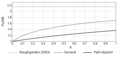
Figure 1: Comparison between PoA($\theta$) in the case of quartic costs for general/path-disjoint networks resp. and the standard bound PoA($\infty$)=$2.1505$ from R03.

Table 1: The Price of Anarchy of free-flow games with non-homogeneous (i.e., with constant terms allowed) polynomial latency functions of maximum degree $p\leq 4$ and minimum degree $q$. Unlabelled bounds are proven in this paper. Bounds for homogeneous (i.e., without constant terms) polynomials can be obtained from the case $\theta=0$ (the same upper bounds have been given in DG06, but tight lower bounds were only conjectured to exist). As it can be appreciated, the PoA depends on the network topology whenever $0<\theta<\infty$. Notes: a: BV20; b: roughgarden2002bad; c: R03.

$(p,q)$ $\theta=0$ $\theta=1/2$ $\theta=1$ $\theta=\infty$ General Path-disjoint General Path-disjoint General Path-disjoint General Path-disjoint $(1,1)$ $1^{a}$ $1$ $1.1547^{a}$ $1.0909$ $1.2071^{a}$ $1.1429$ $1.3333^{b}$ $1.3333^{b}$ $(2,1)$ $1.0355$ $1.0355$ $1.2873$ $1.1472$ $1.3852$ $1.2383$ $1.6258^{c}$ $1.6258^{c}$ $(2,2)$ $1$ $1$ $1.2873$ $1.1472$ $1.3852$ $1.2383$ $1.6258^{c}$ $1.6258^{c}$ $(3,1)$ $1.0982$ $1.0982$ $1.4078$ $1.1869$ $1.5475$ $1.3093$ $1.8956^{c}$ $1.8956^{c}$ $(3,2)$ $1.0147$ $1.0147$ $1.4078$ $1.1869$ $1.5475$ $1.3093$ $1.8956^{c}$ $1.8956^{c}$ $(3,3)$ $1$ $1$ $1.4078$ $1.1869$ $1.5475$ $1.3093$ $1.8956^{c}$ $1.8956^{c}$ $(4,1)$ $1.1676$ $1.1676$ $1.5202$ $1.2170$ $1.6994$ $1.3652$ $2.1505^{c}$ $2.1505^{c}$ $(4,2)$ $1.0450$ $1.0450$ $1.5202$ $1.2170$ $1.6994$ $1.3652$ $2.1505^{c}$ $2.1505^{c}$ $(4,3)$ $1.0080$ $1.0080$ $1.5202$ $1.2170$ $1.6994$ $1.3652$ $2.1505^{c}$ $2.1505^{c}$ $(4,4)$ $1$ $1$ $1.5202$ $1.2170$ $1.6994$ $1.3652$ $2.1505^{c}$ $2.1505^{c}$

1.2 Related Work

Price of Anarchy in routing games: Introduced by KoutsoupiasP99WorstCE, the ratio between the social cost of the worst equilibrium of a game and its optimum was given the name Price of Anarchy (PoA) in (papadimitriou2001algorithms). For networks of linear latency and general topology, PoA was bounded tightly by 4/3 (roughgarden2002bad) and 5/2 in the atomic case (christodoulou2005price). roughgarden2015intrinsic addressed more general latency functions in atomic routing games and again gave tight bounds on PoA. However, for a large class of natural latency functions, PoA tends to 1 as the demand on the network approaches infinitesimally small or infinitely high levels (colini2017asymptotic, Colini2020). This casts doubts on the predictive power of PoA on the state of a real system, as noted in monnot2017routing and (Wu2021).

Other inefficiency metrics widely investigated in selfish routing are the Price of Stability (AnshelevichDKTWR08, ChristodoulouKS11), that compares the best equilibrium of a game with its optimum, and the Price of Risk Aversion (LianeasNM19, KleerS19, FotakisKL20), that takes into account equilibria reached by risk-averse players.

Strategy sets of routing games: They are typically exponential in the number of vertices, hence restricting them is a common assumption. The unnatural character of instances of routing games, which similarly to Pigou’s network exhibit arbitrarily large differences in speeds/latencies between paths, has also been advocated by lu2012worst, who assume players have at least one strategy that is not more than $\lambda$ away from the fastest strategy. Restricting the strategy sets to obtain tighter bounds for PoA is also employed in (bilo2017impact) and (Caragiannis11) for load balancing games (i.e., congestion games where the strategies of players are singleton sets) and for symmetric network congestion games (CorreaJKU19). fotakis2010congestion proved a pure PoA bound for symmetric atomic congestion games on extension-parallel networks, an interesting class of networks with linearly independent paths, that is equal to that of non-atomic congestion games.

Primal-dual techniques for bounding the Price of Anarchy: In non-cooperative games, such techniques have been proposed by B18, KM15, NR10 and T19. The methods proposed in (B18) and (NR10) operate by explicitly formulating the problem of maximizing the Price of Anarchy of a class of games. Despite using the same formulation, they differ in the choice of the variables. While NR10 uses the probability distributions defining the outcomes occurring in the formulation, B18 adopts suitable multipliers for the resource cost functions. The methods in (KM15) and (T19), instead, build on a formulation for the problem of optimizing the social function, and then implement the equilibria conditions within the choice of the dual variables. We adopt the method proposed in (B18) as it appears to be more flexible and powerful in our realm of application. The first advantage is that it generalizes to any type of cost functions, while all the others require some restrictions: the method in (NR10) can only be applied to affine functions, the one in (KM15) requires convex functions, while that of T19 needs non-decreasing ones. Secondly, the method (if properly used) always yields tight bounds on the Price of Anarchy, while those in (KM15) and (T19) are limited by the integrality gap of the formulation. Last but not least, it models in a simple, direct and intuitive way any new twist, as the free-flow property considered in this work, one may want to add to the scenario of application.

Further generalizations or variants of the above primal-dual techniques have been also considered in the context of algorithmic design, with the aim of improving the Price of Anarchy in non-cooperative games (see, for instance, BiloV19, BiloV19stack, PaccagnanCFM21, VijayalakshmiS20). With this respect, PaccagnanCM20 and PaccagnanM22 propose a general primal-dual framework to design the players utility/cost functions so as to optimize the Price of Anarchy, and such functions are defined as solutions of some tractable linear programs.

Transportation research and estimation of Price of Anarchy: The seminal work of Wardrop52 introduces and formalizes one of the first notions of equilibrium in transportation networks. A proof of the equal social costs for equilibria and optimum (i.e., ${\sf{PoA}}=1$) in parallel links routing games appears in (nagurney2009relative). Related ideas from sensitivity analysis for edge cost functions are treated in (tobin1988sensitivity). Similarly, deviations from the perfectly rational user equilibrium have been investigated in Takalloo2020 by quantified the worst-case analytical bounds. Moreover, current technological developments on vehicles’ connectivity and automation have created new opportunities to carefully quantify the actual benefits of large-scale transportation systems. Along the way, several methodological techniques have been proposed to study the magnitude of PoA in real traffic networks, ranging from heuristics (Youn2008) to algorithms of nonconvex optimization (zhang2018price) and to microscopic simulation (Belov2021). For instance, the Price of Anarchy was estimated for the city of Boston with different means from our study by zhang2018price, where the sensitivity of the social cost at equilibrium with respect to edge parameters is also discussed. The previously cited works rely on the BPR estimation of cost functions (bureau1964traffic), which are included in the family of weakly monomial latency functions we define in Section 2. The free-flow property in transportation networks has been first proposed by J+05 with respect to the problem of optimizing a centralized traffic flow without imposing too longer detours to some users.

2 Model and Definitions

For a positive integer $i$, let $[i]:=\{1,2,\ldots,i\}$. Given a set $A$ and a set $B\supseteq A$, let $\chi_{A}:B\rightarrow\{0,1\}$ denote the indicator function, i.e., $\chi_{A}(x)=1$ if $x\in A$ and $\chi_{A}(x)=0$ if $x\notin A$. Given a tuple of numbers $(\alpha_{1},\alpha_{2},\ldots,\alpha_{k})$, we write $(\alpha_{1},\alpha_{2},\ldots,\alpha_{k})>0$ if $\alpha_{i}\geq 0$ for any $i\in[k]$ and $\alpha_{i}>0$ for some $i\in[k]$.

Non-atomic Congestion Games.

A non-atomic congestion game (from now on, simply a congestion game) is a tuple ${\sf CG}=\left([n],(r_{i})_{i\in[n]},E,(\ell_{e})_{e\in E},(\Sigma_{i})_{i\in[n]}\right)$, where $[n]$ is a set of types, $E$ is a set of resources, $\ell_{e}:{\mathbb{R}}_{>0}\rightarrow{\mathbb{R}}_{>0}$ is the latency function of resource $e\in E$, and, for each $i\in[n]$, $r_{i}\in{\mathbb{R}}_{\geq 0}$ is the amount of players of type $i$ and $\Sigma_{i}\subseteq 2^{E}\setminus\emptyset$ is the set of strategies for players of type $i$ (i.e. a strategy is a non-empty subset of resources). We assume that latency functions are non-decreasing, positive, and continuous.

Classes of Congestion Games.

A network congestion game is a congestion game based on a graph $G=(V,E)$, where the set of resources coincides with $E$, each type $i$ is associated with a pair of nodes $(u_{i},v_{i})\in V\times V$, so that the set of strategies of players of type $i$ is the set of paths from $u_{i}$ to $v_{i}$ in graph $G$. If there exists $u^{*}\in V$ such that $u^{*}=u_{i}$ for any $i\in[n]$, the game is called single-source network congestion game. Let $\mathcal{P}$ be the set of all the paths $P$ connecting source $u_{i}$ with destination $v_{i}$, for any pair source-destination $(u_{i},v_{i})$. The game is called path-disjoint network congestion game if all the paths in $\mathcal{P}$ are pair-wise node-disjoint.

A load balancing game is a congestion game in which each strategy is a singleton, i.e., $S=\{e\}$ for some $e\in E$, for any strategy $S\in\Sigma_{i}$ and type $i\in[n]$. A parallel-link game (or symmetric load balancing game) is a load balancing game in which all players have the same set of strategies. It is well-known that each load balancing game (resp. parallel-link game) can be modelled as a single-source congestion game (resp. path-disjoint network congestion game).

Latency Functions.

For the sake of simplicity, we extend the domain of each latency function $\ell(x)$ to $x=0$ in such a way that $\ell(0)=\lim_{x\rightarrow 0^{+}}\ell(x)$. Given a class of latency functions $\mathcal{F}$, let $[\mathcal{F}]_{H}:=\{f:f(x)=g(x)-g(0),\ g\in\mathcal{F}\}$. Observe that $f(0)=0$ for any $f\in[\mathcal{F}]_{H}$ by definition. In the following, we use similar definitions as in (R03). $\mathcal{F}$ is homogeneous if $[\mathcal{F}]_{H}=\mathcal{F}$. $\mathcal{F}$ is weakly diverse if $[\mathcal{F}]_{H}\subseteq\mathcal{F}$ and there exists a constant latency function in $\mathcal{F}$ (i.e., a function $g$ such that $g(x)=\beta$ for any $x$, for some $\beta>0$). $\mathcal{F}$ is scale-closed if it contains all the functions $f$ such that $f(x)=\alpha g(x)$, for any $g\in\mathcal{F}$ and $\alpha>0$. $\mathcal{F}$ is strongly diverse if contains all the functions $f$ such that $f(x)=\alpha g(x)+\beta$, for any $g\in[\mathcal{F}]_{H}$ and $(\alpha,\beta)>0$; observe that, if $\mathcal{F}$ is strongly diverse, then it is both weakly diverse and scale-closed.

A polynomial latency function of maximum degree $p$ and minimum degree $q$ (with $p\geq q\geq 1$) is defined as $\ell_{e}(x):=\sum_{d=q}^{p}\alpha_{e,d}x^{d}+\beta_{e}$, where $(\alpha_{e,q},\alpha_{e,q+1},\ldots,\alpha_{e,p},\beta_{e})>0$. Let $\mathcal{P}_{p,q}$ denote the class of polynomial latency functions of maximum degree $p$ and minimum degree $q$; observe that, if $1\leq q^{\prime}\leq q\leq p\leq p^{\prime}$, then $\mathcal{P}_{p,q}\subseteq\mathcal{P}_{p^{\prime},q^{\prime}}$. A weakly monomial latency function of degree $p$ is defined as $\ell_{e}(x):=\alpha_{e,p}x^{p}+\beta_{e}$, with $(\alpha_{e},\beta_{e})>0$. In the previous definition, $\ell_{e}$ is called monomial latency function of degree $p$ if $\beta_{e}=0$. Let $\mathcal{WM}_{p}$ (resp. $\mathcal{M}_{p}$) denote the class of weakly monomial latency functions (resp. monomial latency functions). Observe that $\mathcal{M}_{p}\subset\mathcal{WM}_{p}=\mathcal{P}_{p,p}$ for any integer $p\geq 1$. A latency function $\ell_{e}$ is affine if $\ell_{e}\in\mathcal{WM}_{1}$, and it is linear if $\ell_{e}\in\mathcal{M}_{1}$.

Strategy Profiles and Pure Nash Equilibria.

A strategy profile is a tuple ${\bm{\sigma}}:=(\sigma_{i,S})_{i\in[n],S\in\Sigma_{i}}$ with $\sum_{S\in\Sigma_{i}}\sigma_{i,S}=r_{i}$ for any $i\in[n]$, that is a state of the game where $\sigma_{i,S}\geq 0$ is the total amount of players of type $i$ selecting strategy $S$ for any $i\in[n]$ and $S\in\Sigma_{i}$. Given a strategy profile ${\bm{\sigma}}$, $k_{e}({\bm{\sigma}}):=\sum_{i\in[n],S\in\Sigma_{i}:e\in S}\sigma_{i,S}$ is the congestion of $e$ in ${\bm{\sigma}}$, i.e., the total amount of players selecting $e$ in ${\bm{\sigma}}$, and given a strategy $S$, $c_{S}({\bm{\sigma}}):=\sum_{e\in S}\ell_{e}(k_{e}({\bm{\sigma}}))$ is the cost of players selecting $S$ in ${\bm{\sigma}}$. A strategy profile ${\bm{\sigma}}$ is a pure Nash equilibrium (or Wardrop equilibrium, or equilibrium flow) if and only if, for each $i\in[n]$, $S\in\Sigma_{i}:\sigma_{i,S}>0$ and $S^{\prime}\in\Sigma_{i}$, it holds that $c_{S}({\bm{\sigma}})\leq c_{S^{\prime}}({\bm{\sigma}})$.

Quality of Equilibria.

A social function that is usually used as a measure of the quality of a strategy profile in congestion games is the total latency, defined as ${\sf SUM}({\bm{\sigma}}):=\sum_{e\in E}k_{e}({\bm{\sigma}})\ell_{e}(k_{e}({\bm{\sigma}}))=\sum_{i\in[n]}r_{i}c_{i}({\bm{\sigma}})$ at equilibrium ${\bm{\sigma}}$. A social optimum is a strategy profile ${\bm{\sigma}}^{*}$ minimizing $\sf SUM$.

The Price of Anarchy of a congestion game $\sf CG$ (with respect to the social function $\sf SUM$), denoted as $\sf{\sf PoA}({\sf CG})$, is the supremum of the ratio ${\sf SUM}({\bm{\sigma}})/{\sf SUM}({\bm{\sigma}}^{*})$, where $\bm{\sigma}$ is a pure Nash equilibrium for $\sf CG$ and ${\bm{\sigma}}^{*}$ is a social optimum for ${\sf CG}$. As shown in roughgarden2002bad, all pure Nash equilibria of any congestion game have the same total latency. Thus, the Price of Anarchy can be redefined as the ratio ${\sf SUM}({\bm{\sigma}})/{\sf SUM}({\bm{\sigma}}^{*})$, where $\bm{\sigma}$ is an arbitrary pure Nash equilibrium for $\sf CG$ and ${\bm{\sigma}}^{*}$ is a social optimum for ${\sf CG}$.

Free-Flow Congestion Games

Given $\theta\in[0,\infty]$, a $\theta$-free-flow congestion game ${\sf CG}_{\theta}$ is a congestion game in which, for each $i\in[n]$ and $S,S^{\prime}\in\Sigma_{i}$, it holds that $\sum_{e\in S}\ell_{e}(0)\leq(1+\theta)\sum_{e\in S^{\prime}}\ell_{e}(0)$, i.e., all the strategies available to players of type $i$, when evaluated in absence of congestion, are within a factor $1+\theta$ one from the other. Observe that free-flow congestion games are congestion games obeying some special properties. Thus, all positive results holding for congestion games carries over to $\theta$-free-flow congestion games for any value of $\theta$. Moreover, for $\theta=\infty$, any congestion game is a $\theta$-free-flow congestion game.

Example 2.1

A simple evidence of how the value of $\theta$ affects the Price of Anarchy of $\theta$-free-flow congestion games, is given by a parallel-link game ${\sf CG}_{c}$ with a unitary amount of players, and two resources $e_{1},e_{2}$ having latency functions defined as $\ell_{1}(x)=1$ and $\ell_{2}(x)=x+c$, for some $c\in[0,1]$. We observe that, for $c=0$, we get the usual Pigou network that matches the worst-case Price of Anarchy of $4/3$ achieved by classical non-atomic congestion games (roughgarden2002bad); however, this network constitutes an extreme case of $\theta$-free-flow congestion games with $\theta=\infty$, since $1+\theta=\ell_{1}(0)/\ell_{2}(0)=1/0=\infty$.

Conversely, if $c>0$, we have that ${\sf CG}_{c}$ is a $\theta$-free-flow congestion game with $\theta=1/c-1$ (since $1+\theta=\ell_{1}(0)/\ell_{2}(0)=1/c$). Furthermore, the Price of Anarchy becomes equal to $4/((c+1)(3-c))<4/3\approx 1.333$, i.e., the social performance increases as $\theta=1/c-1$ decreases. Indeed, the unique equilibrium flow $\bm{\sigma}$ is obtained when all players select resource $e_{1}$, and the social optimum $\bm{\sigma}^{*}$ is obtained when $(1+c)/2$ players select resource $e_{1}$, and the remaining ones select $e_{2}$; thus, by simple calculations, we get

$${\sf{PoA}}({\sf CG})=\frac{{\sf SUM}({\bm{\sigma}})}{{\sf SUM}({\bm{\sigma}}^{*})}=\frac{1}{(c+1)(3-c)/4}=\frac{4}{(c+1)(3-c)}.$$

We observe that, even for $\theta=1$ (attained by $c=1/2$), we get a Price of Anarchy of $16/15\approx 1.066$, thus showing that the equilibrium-flows of the considered congestion game guarantee a social performance that is very close to the optimal one, if the value of $\theta$ is sufficiently small.

3 Price of Anarchy of Free-Flow Congestion Games

In this section, we give tight bounds on the Price of Anarchy of free-flow congestion games. Before going into details, we sketch the high level building blocks of the proofs of the upper bounds. For general $\theta$-free-flow congestion games, by adapting the primal-dual method (B18), we formulate the problem of bounding the Price of Anarchy by means of a factor-revealing pair of primal-dual linear programs. The techniques work as follows.

Given a $\theta$-free-flow congestion game ${\sf CG}_{\theta}$ and a family of latency functions $\mathcal{F}$, we know that we can model the latency of every resource $e\in E$ as $\ell_{e}(x)=\alpha_{e}f_{e}(x)+\beta_{e}$, with $f_{e}\in[\mathcal{F}]_{H}$, $\alpha_{e}\in\{0,1\}$ and $\beta_{e}\geq 0$. We fix a Nash equilibrium ${\bm{\sigma}}$ and a social optimum ${\bm{\sigma}}^{*}$ for ${\sf CG}_{\theta}$. Hence, for every $e\in E$, the congestions $k_{e}({\bm{\sigma}})$ and $k_{e}({\bm{\sigma}}^{*})$ of $e$ in ${\bm{\sigma}}$ and ${\bm{\sigma}}^{*}$, respectively, become fixed constants. As the Price of Anarchy measures the worst-case ratio of ${\sf SUM}({\bm{\sigma}})$ over ${\sf SUM}({\bm{\sigma}}^{*})$, our goal becomes that of choosing suitable values for $\alpha_{e}$ and $\beta_{e}$, for every $e\in E$, so as to maximize ${\sf SUM}({\bm{\sigma}})$ under the assumption that ${\sf SUM}({\bm{\sigma}}^{*})=1$, ${\bm{\sigma}}$ is a Nash equilibrium and ${\sf CG}_{\theta}$ is a $\theta$-free-flow game. In particular, constraint ${\sf SUM}({\bm{\sigma}}^{*})=1$ can be assumed without loss of generality by a simple scaling argument, provided we relax the condition $\alpha_{e}\in\{0,1\}$ with $\alpha_{e}\geq 0$. Thus, an optimal solution to the resulting linear program, call it LP, provides an upper bound to the Price of Anarchy of ${\sf CG}_{\theta}$.

Next step is to compute and analyze the dual of LP, that we call DLP. DLP has three variables, namely $x$, $y$ and $\gamma$, with $x\geq 0$, $y\geq 0$ and $\gamma$ defining its objective value. Thus, by the Weak Duality Theorem, any feasible solution $(x,y,\gamma)$ for DLP yields an upper bound of $\gamma$ to the optimal solution of LP and so an upper bound to the Price of Anarchy of ${\sf CG}_{\theta}$. For each resource $e\in E$, DLP has two constraints, namely $c_{1}(f_{e},k_{e}({\bm{\sigma}}),k_{e}({\bm{\sigma}}^{*}),x,\gamma)$ and $c_{2}(f_{e},k_{e}({\bm{\sigma}}),k_{e}({\bm{\sigma}}^{*}),y,\gamma)$, respectively associated to the primal variables $\alpha_{e}$ and $\beta_{e}$, and providing lower bounds on $\gamma$. In particular, we consider a feasible solution $(x^{*},y^{*},\gamma^{*})$ that is optimal for DLP, under the further constraints $y=\frac{x-1}{1+\theta}$ and $x\geq 1$. Then, by exploiting the dual constraints, we obtain two significant lower bounds for $\gamma^{*}$; both bounds depend on the structural properties of the latency functions $f_{e}$; moreover, the first bound is also influenced by the choice of the optimal dual variable $x$ (i.e., $x^{*}$), while the second exhibits a dependence from $\theta$. For any class of latency functions $\mathcal{G}$, by using $k$ and $l$ as a shorthand for $k_{e}({\bm{\sigma}})$ and $k_{e}({\bm{\sigma}}^{*})$, respectively, these lower bounds bounds for $\gamma^{*}$ are at most equal to $\gamma([\mathcal{F}]_{H})$ and $\gamma_{\theta}([\mathcal{F}]_{H})$, with

$$\gamma(\mathcal{G}):=\inf_{x>1}\sup_{k>0,l>0,f\in\mathcal{G}}\left(\frac{k+x(-k+l)}{l}\right)\frac{f(k)}{f(l)},$$ (1)

$$\gamma_{\theta}(\mathcal{G}):=\sup_{k>l>0,f\in\mathcal{G}}\frac{(k-l)f(k)+kf(k)\theta}{(k-l)f(k)+[(k-l)f(k)+lf(l)]\theta};$$ (2)

thus the maximum value between $\gamma([\mathcal{F}]_{H})$ and $\gamma_{\theta}([\mathcal{F}]_{H})$ is an upper bound on the optimal solution of DLP, and then an upper bound on the Price of Anarchy (see Theorem 3.3).

Remark 3.1

Given a class of latency functions $\mathcal{G}$, we observe that $\gamma(\mathcal{G})$ is at least equal to 1; to show this, it is sufficient setting $k=l$ in the quantities of which the supremum is taken (when defining $\gamma(\mathcal{G})$). Furthermore, we observe that $\gamma_{\theta}(\mathcal{G})=1$ for $\theta=0$ and that $\gamma_{\theta}(\mathcal{G})$ is non-decreasing in $\theta\geq 0$.

An important advantage of the primal-dual method is that, whenever LP provides a tight characterization of the properties possessed by the games and the equilibria under analysis, an optimal solution to DLP can be fruitfully exploited to construct, quite systematically, but not without effort, matching lower bounding instances. We manage to achieve this result also in this case, but, given the very technical nature of the constructions, we refer the interested reader to the appendix.

In the related literature, bounds on the Price of Anarchy are often obtained by exploiting Roughgarden’s smoothness framework (roughgarden2015intrinsic)Other variants of the smoothness framework are introduced and applied in (Bach2014, Chan2019, Roug15b, Roug2017).. It is based on an inequality linking together the social value of an optimal solution and the sum of the players’ costs at an equilibrium, thus requiring the use of two variables. However, for certain settings, as the one considered in this work, additional structural properties of the game need to be embedded in the model. This requires more sophisticated constraints involving a higher number of variables. The primal-dual method handles these twists more easily, as it suffices writing down properly all the additional constraints that need to be satisfied by the model (in our case, the free-flow property). Then, the final set of factor-revealing inequalities that needs to be analyzed elegantly results as a consequence of the duality theory.

For the case of parallel-link and path-disjoint games, we apply a similar, although more direct approach. We fix once again ${\sf CG}_{\theta}$, the family of latency functions $\mathcal{F}$, the latency of every resource $e\in E$, a Nash equilibrium ${\bm{\sigma}}$ and a social optimum ${\bm{\sigma}}^{*}$ for ${\sf CG}_{\theta}$, so as to obtain constant values for both $k_{e}({\bm{\sigma}})$ and $k_{e}({\bm{\sigma}}^{*})$. This time, instead of resorting to linear programming, we write down the parametric expression of the Price of Anarchy as a function of $k_{e}({\bm{\sigma}})$, $k_{e}({\bm{\sigma}}^{*})$ and the latency functions of the resources in the game. A key feature of this case, that makes it different from the general setting analyzed before, is that, here, we need have $\sum_{e\in E}k_{e}({\bm{\sigma}})=\sum_{e\in E}k_{e}({\bm{\sigma}}^{*})$. By exploiting this equality, together with the equilibrium conditions and the $\theta$-free-flow property of ${\sf CG}_{\theta}$, we create a sequence of more and more relaxed upper bounds for the Price of Anarchy, until we end up to a sufficiently simple formula. In particular, let

$$\eta_{\theta}(\mathcal{G}):=\sup_{k>l>0,f\in\mathcal{G}}\frac{kf(k)+kf(k)\theta}{kf(k)+[(k-l)f(k)+lf(l)]\theta};$$ (3)

we show that the maximum value between $\gamma([\mathcal{F}]_{H})$ and $\eta_{\theta}([\mathcal{F}]_{H})$ is an upper bound on the Price of Anarchy (see Theorem 3.6).

Remark 3.2

Given a class of latency functions $\mathcal{G}$, we observe that $\eta_{0}(\mathcal{G})=1$ and that $\eta_{\theta}(\mathcal{G})$ is non-decreasing in $\theta\geq 0$. Furthermore, we observe that $\eta_{\theta}(\mathcal{G})\leq\gamma_{\theta}(\mathcal{G})$ for any $\theta\geq 0$.

Also in this case, we can show that the performed analysis is tight by providing matching lower bounding instances whose description is again deferred to the appendix.

For the sake of simplicity, the case $\theta=\infty$ (i.e., congestion games without the free-flow hypothesis) is not considered in the main theorems, as it has been already treated by some previous works (R03, C+04) under similar hypothesis on the latency functions. Anyway, we separately treat the case $\theta=\infty$ in a corollary of the main theorems (see Corollary 3.5), to provide better bounds on the Price of Anarchy (with respect to the existing ones) under weaker hypothesis on the considered classes of latency functions (see Subsection LABEL:sub_int_1 for further details).

3.1 The Main Theorems

Theorem 3.3

Let ${\sf CG}_{\theta}$ be a $\theta$-free-flow congestion game with latency functions in $\mathcal{F}$ and $\theta\geq 0$. Then ${\sf{PoA}}({\sf CG}_{\theta})\leq\max\{{\gamma}([\mathcal{F}]_{H}),{\gamma}_{\theta}([\mathcal{F}]_{H})\}$. Furthermore, this bound is tight for single-source network games if $\mathcal{F}$ is weakly diverse, and even for (non-symmetric) load balancing games if $\mathcal{F}$ is strongly diverse.

Proof 3.4

Proof: Let ${\bm{\sigma}}=(\sigma_{i,S})_{i\in[n],S\in\Sigma_{i}}$ and ${\bm{\sigma}}^{*}=(\sigma_{i,S}^{*})_{i\in[n],S\in\Sigma_{i}}$ be a pure Nash equilibrium and a social optimum for ${\sf CG}_{\theta}$, respectively. Let $k_{e}:=k_{e}({\bm{\sigma}})$ and $l_{e}:=k_{e}({\bm{\sigma}}^{*})$ for any $e\in E$. Let $\ell_{e}(x):=\alpha_{e}f_{e}(x)+\beta_{e}$ be the latency function of each resource $e\in E$, with $\alpha_{e}\in\{0,1\}$, $\beta_{e}\geq 0$, and $f_{e}\in[\mathcal{F}]_{H}$. By applying the primal-dual method (B18), we have that the optimal solution of the following linear program in variables $(\alpha_{e})_{e\in E}$ and $(\beta_{e})_{e\in E}$ is an upper bound on ${\sf{PoA}}({\sf CG}_{\theta})$:

$${\sf LP:}\ \max\ \sum_{e\in E}(\alpha_{e}k_{e}f_{e}(k_{e})+\beta_{e}k_{e})$$

s.t. $$\sum_{e\in E}(\alpha_{e}k_{e}f_{e}(k_{e})+\beta_{e}k_{e})\leq\sum_{e\in E}(\alpha_{e}l_{e}f_{e}(k_{e})+\beta_{e}l_{e})$$ (4)

$$\sum_{e\in E}\beta_{e}l_{e}\leq\sum_{e\in E}(1+\theta)\beta_{e}k_{e}$$ (5)

$$\sum_{e\in E}(\alpha_{e}l_{e}f_{e}(l_{e})+\beta_{e}l_{e})=1$$ (6)

$$\alpha_{e},\beta_{e}\geq 0\quad\forall e\in E.$$

Indeed:

$\bullet$ Objective function:

Each latency function $\ell_{e}$ can be expressed as $\ell_{e}(k_{e})=\alpha_{e}f_{e}(k_{e})+\beta_{e}$ with $\alpha_{e}\in\{0,1\}$.

$\bullet$ Constraint (4):

For any $i\in[n]$, and any two strategies $S,S^{*}\in\Sigma_{i}$, let $\sigma_{i,S,S^{*}}\geq 0$ denote the amount of players of type $i$ selecting $S$ in ${\bm{\sigma}}$ and selecting $S^{*}$ in ${\bm{\sigma}}^{*}$. By the pure Nash equilibrium conditions, we have that $\sum_{e\in S}(\alpha_{e}f_{e}(k_{e})+\beta_{e})\leq\sum_{e\in S^{*}}(\alpha_{e}f_{e}(k_{e})+\beta_{e})$, for any $i\in[n]$, and for any two strategies $S,S^{*}\in\Sigma_{i}$ such that $\sigma_{i,S,S^{*}}>0$. Then, we have that

$$0 \geq\sum_{i\in[n]}\sum_{S,S^{*}\in\Sigma_{i}}\sigma_{i,S,S^{*}}\left(\sum_{e\in S}(\alpha_{e}f_{e}(k_{e})+\beta_{e})-\sum_{e\in S^{*}}(\alpha_{e}f_{e}(k_{e})+\beta_{e})\right)$$

$$=\sum_{e\in E}\left(\sum_{i\in[n],S,S^{*}\in\Sigma_{i}:e\in S}\sigma_{i,S,S^{*}}\right)(\alpha_{e}f_{e}(k_{e})+\beta_{e})-\sum_{e\in E}\left(\sum_{i\in[n],S,S^{*}\in\Sigma_{i}:e\in S^{*}}\sigma_{i,S,S^{*}}\right)(\alpha_{e}f_{e}(k_{e})+\beta_{e})$$

$$=\sum_{e\in E}\left(\sum_{i\in[n],S\in\Sigma_{i}:e\in S}\sum_{S^{*}\in\Sigma_{i}}\sigma_{i,S,S^{*}}\right)(\alpha_{e}f_{e}(k_{e})+\beta_{e})-\sum_{e\in E}\left(\sum_{i\in[n],S^{*}\in\Sigma_{i}:e\in S^{*}}\sum_{S\in\Sigma_{i}}\sigma_{i,S,S^{*}}\right)(\alpha_{e}f_{e}(k_{e})+\beta_{e})$$

$$=\sum_{e\in E}\left(\sum_{i\in[n],S\in\Sigma_{i}:e\in S}\sigma_{i,S}\right)(\alpha_{e}f_{e}(k_{e})+\beta_{e})-\sum_{e\in E}\left(\sum_{i\in[n],S^{*}\in\Sigma_{i}:e\in S^{*}}\sigma_{i,S^{*}}\right)(\alpha_{e}f_{e}(k_{e})+\beta_{e})$$

$$=\sum_{e\in E}(\alpha_{e}k_{e}f_{e}(k_{e})+\beta_{e}k_{e})-\sum_{e\in E}(\alpha_{e}l_{e}f_{e}(k_{e})+\beta_{e}l_{e}),$$

and this implies constraint (4).

$\bullet$ Constraint (5):

By using the definition of $\theta$-free-flow congestion games, we have that $\sum_{e\in S^{*}}\beta_{e}\leq(1+\theta)\sum_{e\in S}\beta_{e}$, for any $i\in[n]$, and for any strategies $S,S^{*}\in\Sigma_{i}$ such that $\sigma_{i,S,S^{*}}>0$. Thus

$$0 \geq\sum_{i\in[n]}\sum_{S,S^{*}\in\Sigma_{i}}\sigma_{i,S,S^{*}}\left(\sum_{e\in S^{*}}\beta_{e}-(1+\theta)\sum_{e\in S}\beta_{e}\right)$$

$$=\sum_{e\in E}\left(\sum_{i\in[n],S,S^{*}\in\Sigma_{i}:e\in S^{*}}\sigma_{i,S,S^{*}}\right)\beta_{e}-(1+\theta)\sum_{e\in E}\left(\sum_{i\in[n],S,S^{*}\in\Sigma_{i}:e\in S}\sigma_{i,S,S^{*}}\right)\beta_{e}$$

$$=\sum_{e\in E}\left(\sum_{i\in[n],S^{*}\in\Sigma_{i}:e\in S^{*}}\sigma_{i,S^{*}}\right)\beta_{e}-(1+\theta)\sum_{e\in E}\left(\sum_{i\in[n],S\in\Sigma_{i}:e\in S}\sigma_{i,S}\right)\beta_{e}$$

$$=\sum_{e\in E}l_{e}\beta_{e}-\sum_{e\in E}(1+\theta)k_{e}\beta_{e},$$

and this implies constraint (5).

$\bullet$ Constraint (6) + Relaxations:

The Price of Anarchy of ${\sf CG}_{\theta}$ is $\frac{{\sf SUM}({\bm{\sigma}})}{{\sf SUM}({\bm{\sigma}}^{*})}=\frac{\sum_{e\in E}(\alpha_{e}k_{e}f_{e}(k_{e})+\beta_{e}k_{e})}{\sum_{e\in E}(\alpha_{e}l_{e}f_{e}(l_{e})+\beta_{e}l_{e})}$, thus, by maximizing such value over all the possible $\alpha_{e},\beta_{e}\geq 0$ subject to constraints (4) and (5), we get an upper bound on the Price of Anarchy of ${\sf CG}_{\theta}$. If we restrict the values of $\alpha_{e}$ and $\beta_{e}$ in such a way that the further normalization constraint (6) holds, we do not affect the maximum value considered above, thus finding such maximum value is equivalent to find the optimal solution of LP. This can be achieved by relaxing the condition $\alpha_{e}\in\{0,1\}$ to $\alpha_{e}\geq 0$.

We call generating set a generic finite set $\mathcal{T}\subseteq\{(k,l,f):k,l\geq 0,f\in[\mathcal{F}]_{H}\}$. For any generating set $\mathcal{T}$, we define a linear program in variables $\gamma,x,y$:

$${\sf DLP}(\mathcal{T})\quad\min\quad \gamma$$

s.t. $$lf(l)\gamma\geq kf(k)+x(-kf(k)+lf(k))\quad\forall(k,l,f)\in\mathcal{T}$$ (7)

$$l\gamma\geq k+x(-k+l)+y(-l+(1+\theta)k)\quad\forall(k,l,f)\in\mathcal{T}$$ (8)

$$x,y\geq 0,$$

Let $\mathcal{T}_{E}:=\{(k_{e},l_{e},f_{e}):e\in E\}$. Observe that ${\sf DLP}(\mathcal{T}_{E})$ is the dual of LP. Indeed, for $\mathcal{T}=\mathcal{T}_{E}$, each dual constraint of type (7) (resp. (8)) is associated to some primal variable $\alpha_{e}$ (resp. $\beta_{e}$), and $x$ (resp. $y$, resp. $\gamma$) is the dual variable associated to the primal constraint defined in (4) (resp. (5), resp. (6)).

By the Weak Duality Theorem, any feasible solution $(x,y,\gamma)$ of ${\sf DLP}(\mathcal{T}_{E})$ is such that $\gamma$ is at least equal to the optimal value of LP, that is an upper bound on ${\sf{PoA}}({\sf CG}_{\theta})$. Thus, to show the claim, it is sufficient providing, for any generating set $\mathcal{T}$, a tuple $(x,y,\gamma)$ with $\gamma\leq\max\{{\gamma}([\mathcal{F}]_{H}),{\gamma}_{\theta}([\mathcal{F}]_{H})\}$ that is a feasible solution of ${\sf DLP}(\mathcal{T})$.

Let $\mathcal{T}$ be an arbitrary generating set. Let $(x^{*},y^{*},\gamma^{*})$ be the optimal solution of ${\sf DLP}(\mathcal{T})$, subject to the further constraints $x\geq 1$ and $y:=\frac{x-1}{1+\theta}$. Under the above (further) constraints on ${\sf DLP}(\mathcal{T})$, we have that the constraints of type (7) and (8) of ${\sf DLP}(\mathcal{T})$ are satisfied by any value of $\gamma$ if $l=0$, thus we can assume without loss of generality that $l$ is always positive. We conclude that $(x^{*},\gamma^{*})$ is the optimal solution of the following linear program:

$${\sf DLP2}(\mathcal{T}):\quad\min\ \gamma$$

s.t. $$\gamma\geq\frac{kf(k)+x(-kf(k)+lf(k))}{lf(l)},\ \forall(k,l,f)\in\mathcal{T}:l>0$$ (9)

$$\gamma\geq\frac{x\theta+1}{1+\theta}$$ (10)

$$x\geq 1,$$ (11)

where (10) is obtained by imposing $y:=\frac{x-1}{1+\theta}$ and $l>0$ in (8).

First of all, we assume that $(x^{*},\gamma^{*})$ is such that constraint (10) is not tight. In such case, we have that $(x^{*},\gamma^{*})$ continues to be the optimal solution of a linear program obtained from ${\sf DLP2}(\mathcal{T})$ by deleting constraint (10). Thus, we getEquality (13) holds since, by continuity, the supremum over $k>0$ is equal to that over $k\geq 0$.

$${\sf{PoA}}({\sf CG}_{\theta}) \leq\gamma^{*}$$ (12)

$$=\max_{(k,l,f)\in\mathcal{T}:l>0}\frac{kf(k)+x^{*}(-kf(k)+lf(k))}{lf(l)}$$

$$=\min_{x\geq 1}\max_{(k,l,f)\in\mathcal{T}:l>0}\frac{kf(k)+x(-kf(k)+lf(k))}{lf(l)}$$

$$\leq\inf_{x\geq 1}\sup_{k\geq 0,l>0,f\in[\mathcal{F}]_{H}}\frac{kf(k)+x(-kf(k)+lf(k))}{lf(l)}$$

$$=\inf_{x\geq 1}\sup_{k>0,l>0,f\in[\mathcal{F}]_{H}}\frac{kf(k)+x(-kf(k)+lf(k))}{lf(l)}$$ (13)

$$\leq\inf_{x>1}\sup_{k>0,l>0,f\in[\mathcal{F}]_{H}}\frac{kf(k)+x(-kf(k)+lf(k))}{lf(l)}$$

$$={\gamma}([\mathcal{F}]_{H}),$$ (14)

and the claim follows when constraint (10) is not tight under solution $(x^{*},\gamma^{*})$.

Now, we assume that $(x^{*},\gamma^{*})$ is such that constraint (10) is tight, i.e., $\gamma^{*}=\frac{x^{*}\theta+1}{1+\theta}$. As ${\sf DLP2}(\mathcal{T})$ has three variables, we have that the optimal solution $(x^{*},\gamma^{*})$ can be chosen in such a way that a further constraint is tight. If such tight constraint is (11), i.e., $x^{*}=1$ holds, by exploiting constraint (10) we get $\gamma^{*}=1$; thus ${\sf{PoA}}({\sf CG}_{\theta})\leq\gamma^{*}=1\leq{\gamma}_{\theta}([\mathcal{F}]_{H})$, and the claim follows. If the further tight constraint is (9) for some triple $(k,l,f)\in\mathcal{T}$, we have that pair $(x^{*},\gamma^{*})$ satisfies equations $\gamma^{*}=\frac{kf(k)+x^{*}(-kf(k)+lf(k))}{lf(l)}$ and $\gamma^{*}=\frac{x^{*}\theta+1}{1+\theta}$, that is, $\gamma^{*}=\frac{(k-l)f(k)+kf(k)\theta}{(k-l)f(k)+[(k-l)f(k)+lf(l)]\theta}$. Thus, we get

$${\sf{PoA}}({\sf CG}_{\theta}) \leq\gamma^{*}$$

$$=\frac{(k-l)f(k)+kf(k)\theta}{(k-l)f(k)+[(k-l)f(k)+lf(l)]\theta}$$

$$\leq\sup_{k>l>0,f\in[\mathcal{F}]_{H}}\frac{(k-l)f(k)+kf(k)\theta}{(k-l)f(k)+[(k-l)f(k)+lf(l)]\theta}$$

$$={\gamma}_{\theta}([\mathcal{F}]_{H}),$$ (15)

and this concludes the proof for the upper bound.

The construction of the matching lower bounding instances is deferred to the appendix.

By using the same proof arguments of the above theorem, we get the following corollary (whose proof is deferred to the appendix), that provides tight bounds on the Price of Anarchy for classical congestion games (i.e., without the $\theta$-free-flow hypothesis).

Corollary 3.5

The Price of Anarchy of congestion games with latency functions in $\mathcal{F}$ is at most $\gamma(\mathcal{F})$. Furthermore, this bound is tight for parallel-link games if $\mathcal{F}$ is scale-closed, and is tight for path-disjoint network-congestion games if $\mathcal{F}$ is arbitrary.

We now show that, when considering either parallel-link games or path-disjoint network congestion games, a better bound on the Price of Anarchy can be achieved.

Theorem 3.6

Let ${\sf PLG}_{\theta}$ be a $\theta$-free-flow path-disjoint network congestion game with latency functions in $\mathcal{F}$ and $\theta\geq 0$. Then ${\sf{PoA}}({\sf PLG}_{\theta})\leq\max\{{\gamma}([\mathcal{F}]_{H}),{\eta}_{\theta}([\mathcal{F}]_{H})\}$. Furthermore, this bound is tight if $\mathcal{F}$ is weakly diverse, and even for parallel-link games if $\mathcal{F}$ is strongly diverse.