A Systematic Method for On-The-Fly Denormalization of Relational Databases
Abstract – Normalized relational databases are a common method for storing data, but pulling out usable denormalized data for consumption generally requires either direct access to the source data or creation of an appropriate view or table by a database administrator. End-users are thus limited in their ability to explore and use data that is stored in this manner. Presented here is a method for performing automated denormalization of relational databases at run-time, without requiring access to source data or ongoing intervention by a database administrator. Furthermore, this method does not require a restructure of the database itself and so it can be flexibly applied as a layer on top of already existing databases.
Introduction
Normalized relational databases took their form initially from a need to reduce duplication of records and to organize data in a manner whereby updating or adding records would not lead to data inconsistencies [1]. However, this structure can lead to difficulty with the actual retrieval of usable information. For wide databases, it can be an arduous process to discover the logical sequence of tables that must be joined to bring information from different ends of the database together, especially when many combinations of different data elements are desired. A more important limitation is that an end-user of the data without direct access is reliant upon the database administrator creating the denormalized tables a priori for any data exploration/analysis desired.
Relational databases remain the most common method of storing data [2]. Data collected for research purposes are also usually stored/provided using a relational schema. Thus, there is a role for creating a technique for on-the-fly denormalization, to allow for maximal flexibility for information retrieval by end-users and to unburden the database administrator. The algorithms provided here will enable an end-user to be able to combine any number of columns of interest from any number of tables, and automatically construct the join sequences required to perform this denormalization ad hoc.
Illustrative Example
We will use a modified version of the Northwind Traders database to demonstrate scenarios where an on-the-fly denormalization algorithm can be useful. The Northwind Traders database was originally created by the Microsoft Corporation, and the modified files can be found at https://github.com/sareeneng/NorthwindModified. The modified dataset consists of 11 tables that are organized in a typical normalized fashion, although some of the relationships have been constructed in a way to highlight certain points in the discussion to follow, and so it is not a fully optimized data representation. For simplicity, only the joining columns and a few other columns are shown in Figure 1.
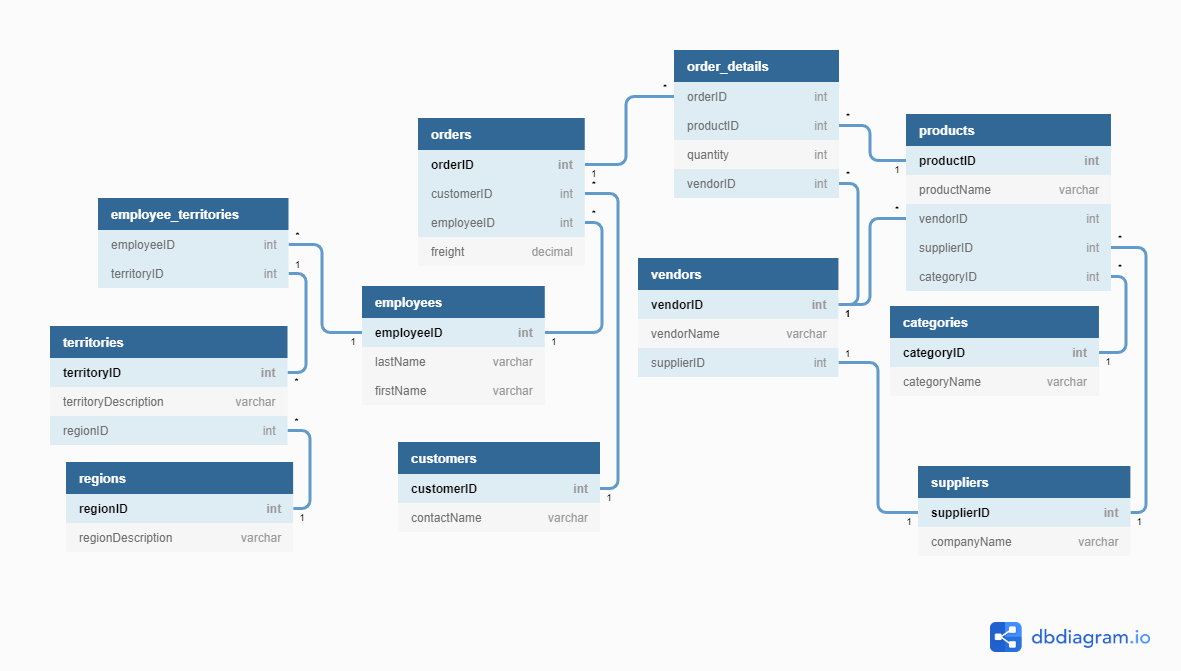
Suppose an end-user is interested in finding which employees and customers have interacted with each other. From the diagram, it is clear that the way to accomplish this is to start with the orders table, and then join the employees and customers tables in. A database administrator might create a view to bring the data from these two tables together if this is a frequently requested combination of variables. This requires anticipation on the part of the administrator.
If the end-user wants to explore the database and create many different combinations of variables, then these must also be anticipated. For example, the user might want to know what territories the orders are originating from, or see which vendors served which customers. The user may also want many more variables pulled in together, such as quantity and names of the products sold by each employee. Notably, some of these combinations may not be possible; orders are linked to employees, but employees may serve multiple territories so there is no way to definitively link the tables territories to orders.
One (unfeasible) option is to anticipate all potential combinations that a user may be interested in and create the associated denormalized tables (e.g. with a star schema). This becomes an exponentially laborious task the wider the database and the more variables that a user might want to pull together, and the vast majority of these cases will be extraneous. The on-the-fly denormalization algorithm presented here avoids the need to anticipate end-user data requests.
Graph Structure
A simple way to represent the relational database is by using a directed graph structure that will then allow for the path-finding required. Tables are represented as the nodes, and foreign key links are represented as the edges between nodes. The box details the steps for constructing the graph, and Figure 2 shows the resulting graph for the modified Northwind dataset.
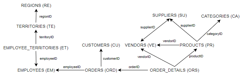
The columns used to join tables together can be classified as either “many” (non-unique values) or “one” (only unique values). The method for determining whether the columns have only unique values will depend on the database management system. The links between tables can then be manually specified, and the directionality of the arrows determined based on the columns classification in both tables. In the case where there are multiple foreign keys between two tables, linking options will depend on the use-case. A database administrator may decide that only one of the foreign keys is relevant, or all links may be created and an option may be provided to the user at run-time as to which specific connection to use for the query.
There are a few ways to minimize the amount of manual labor involved in creating these links, including:
-
1.
If the database is stored in a typical database management system with foreign keys already set up, then these foreign keys can be used to create the connections.
-
2.
Many databases are structured such that column names have a consistent meaning across tables. In this case, one can iterate over all column names and whenever a column is found in multiple tables, then a link can be created with directionality based on the classification described above if the uniqueness of the columns is known and will not change.
Once the graph has been created, then the connections can be stored and the graph regenerated from this metadata at any time. At this point, two path-finding algorithms need to be implemented:
-
1.
Find if a path exists at all between any two nodes.
-
2.
Find all simple paths between any two nodes - a simple path is one that connects the source to the target without traversing any interceding nodes more than once.
Many programming languages have packages/modules that can construct these graphs and implement the path-finding algorithms needed. For example, Python users can install the networkx package [3].
Denormalization Algorithm
The basic algorithm builds on the idea that one needs to find an origin node from which a simple path can be drawn to all individual desired nodes. The origin node may also be one of the desired nodes. For example, if the user is interested in data from the suppliers and the categories tables, a path cannot be drawn directly from one to the other. However, the origin node products has a path to each individual desired table, and so it can serve as the left-most table in the join sequence. There is the potential for a significant amount of redundancy; order_details could have served as an origin node, but it does not add more useful information and adds more complexity if the user is only interested in suppliers and categories, while products is a necessary table in the join sequence. The steps below describe how to eliminate the redundancy.
Find paths between two given tables
The first building block is to find all simple paths between an origin node and each desired table. Some of the paths found may include extraneous tables (which may reduce useful information while adding to complexity), and so the redundancy should be removed (Algorithm 1). First, sort the list of paths found from shortest to longest, then eliminate all paths that are a superset of any previous path. For example, the simple paths from order_details to suppliers are , , and . The first two paths are kept because neither is a superset of the other, and it is unknown at this time which is the optimal path (e.g. going through vendors might yield more rows or more relevant data than going through products, or vice-versa). However the last path can be removed because there is no possibility of it being more optimal than either of the first two paths.
Note that this is not the same as finding edge disjoint paths. If one path is and another is , these paths share an edge but it is not clear if one is inferior to the other and so both should be kept.
Finding join sequences between multiple tables
If an origin node exists from which a simple path can be drawn to all desired nodes, then at least one join sequence can be generated. The basic technique is to first take all the paths between all possible origin nodes and each of the desired tables. The origin node might be one of the desired nodes. Then calculate the cartesian product to generate all possible valid combinations of simple paths, and in a similar fashion as above, sort the candidate join sequences by the number of unique tables to remove those that are simply supersets of prior sequences. These steps are outlined in Algorithm 2.
The operation of finding all simple paths can be computationally expensive for very large graphs. A significant optimization can be done by first checking to see if a path exists at all from the candidate origin node to each of the desired nodes using Dijkstra’s algorithm, and if not, then move on to the next candidate.
The result will be a list of lists, with each individual list comprised of a set of ordered pairs representing a join sequence. For example: , represents “ JOIN ON JOIN ON JOIN …” . For brevity, the above can also be represented as
A fully worked example is provided in the Appendix, where a join sequence is found between customers, suppliers, and categories. Note that this is different from the examples provided above in order to specifically highlight all the steps of the algorithm. The join sequence generated by this algorithm uses the order_details table as the origin/left-most table. Of note, the algorithm eliminates the potential join sequence that makes use of the path from because in order to capture categories, the products table must be included and since suppliers is directly related to products, there is no need to use vendors. If categories was not required, then two valid join sequences would have been produced.
Discussion
The algorithm presented here allows for end-user creation and consumption of denormalized data without requiring a restructuring of the normalized database and without requiring access to the source data. Once the initial set-up has been completed by a database administrator, data can be pulled from different tables with the appropriate joins created automatically through the steps detailed above. Furthermore, this algorithm is relatively simple to implement in various programming languages. A plausible use-case scenario could be a dashboard where an end-user can select data elements of interest and choose filters, and then the resulting denormalized data can be used to construct visualizations.
There are several limitations, some of which have been described above.
-
•
The links need to be set up manually, but this is a one-time task. Ideally this should be done by an administrator familiar with the database structure (especially if the database is live) as this person can identify which are the important links between tables, and classify the relationships appropriately based on defined constraints and foreign keys. If the data is provided as static files and there is no database administrator (e.g. research data provided for distribution in .csv format), then the column data itself can be analyzed to determine if there are unique/non-unique values present, and then the appropriate relationships can be set up.
-
•
For very large and highly connected graphs, the path-finding may be computationally expensive. Some options to ameliorate this include storing the paths when found to avoid having to recalculate them, ensuring a path exists using Djikstra’s algorithm, and setting a maximum search depth. Once the paths have been found for a pair of nodes, they can be stored for future use so that they do not need to be recalculated every time.
-
•
There is no specific support for self-referencing tables, though the algorithm could be modified to incorporate this.
-
•
In the case where there are multiple valid join sequences, a decision needs to be made on which data to provide. Options are to 1) prioritize paths that traverse mandatory over optional foreign keys, 2) provide the “union distinct” output of all possible results, 3) provide each result separately, or 4) provide the table that has the most records in it.
Acknowledgments
I would like to thank Dr. Alysia Flynn for her thorough review and analysis of the algorithm, as well as Dr. Nelson Sanchez-Pinto for his guidance and mentorship.
References
- [1] S. Malaika and M. Nicola, “The history of business records.” https://www.ibm.com/developerworks/data/library/techarticle/dm-1112normalization/index.html, Dec 2011.
- [2] solid IT, “Historical trend of the popularity ranking of database management systems.” https://db-engines.com/en/ranking_trend, Sept 2020.
- [3] Networkx developers, “Networkx documentation.” https://networkx.github.io/, 2020.
Appendix
Worked Example
Find a join sequence between customers, suppliers, and categories (from Figure 1)
-
1.
=
-
2.
=
-
3.
-
•
, this is the only simple path.
-
•
no simple paths found. Stop and move onto the next candidate origin node.
-
•
-
•
-
•
-
•
-
•
nodes set is which is a superset of the nodes in so eliminate it. Note that it is also a superset of but the first condition is enough to eliminate.
-
•
-
•
-
•
Add and to
have at least one , so no new valid join sequences are found in this case, and is fully populated from as the origin node. -
•
-
4.
has 6 unique nodes
has 7 unique nodes -
5.
The nodes in are a superset of the nodes in and so it can be eliminated. This leave only one join sequence:
which can be translated as follows:
JOIN ON JOIN ON JOIN ON JOIN ON JOIN ON