Resolved spectral variations of the centimetre-wavelength continuum from the $\rho$ Oph W photo-dissociation-region

Abstract

Cm-wavelength radio continuum emission in excess of free-free, synchrotron and Rayleigh-Jeans dust emission (excess microwave emission, EME), and often called ‘anomalous microwave emission’, is bright in molecular cloud regions exposed to UV radiation, i.e. in photo-dissociation regions (PDRs). The EME correlates with IR dust emission on degree angular scales. Resolved observations of well-studied PDRs are needed to compare the spectral variations of the cm-continuum with tracers of physical conditions and of the dust grain population. The EME is particularly bright in the regions of the $\rho$ Ophiuchi molecular cloud ($\rho$ Oph) that surround the earliest type star in the complex, HD 147889, where the peak signal stems from the filament known as the $\rho$ Oph-W PDR. Here we report on ATCA observations of $\rho$ Oph-W that resolve the width of the filament. We recover extended emission using a variant of non-parametric image synthesis performed in the sky plane. The multi-frequency 17 GHz to 39 GHz mosaics reveal spectral variations in the cm-wavelength continuum. At $\sim$30 arcsec resolutions, the 17-20 GHz intensities follow tightly the mid-IR, $I_{\mathrm{cm}}\propto I(8\,\mu$m), despite the breakdown of this correlation on larger scales. However, while the 33-39 GHz filament is parallel to IRAC 8 $\mu$m, it is offset by 15–20 arcsec towards the UV source. Such morphological differences in frequency reflect spectral variations, which we quantify spectroscopically as a sharp and steepening high-frequency cutoff, interpreted in terms of the spinning dust emission mechanism as a minimum grain size $a_{\mathrm{cutoff}}\sim 6\pm 1\,$Å that increases deeper into the PDR.

1 Introduction

Cosmic microwave background anisotropy experiments have identified an anomalous diffuse foreground in the range of 10-90 GHz (Kogut et al., 1996; Leitch et al., 1997), which was confirmed, in particular, by the WMAP (e.g. Gold et al., 2011) and Planck missions (e.g. Planck Collaboration et al., 2016a). As summarised in Dickinson et al. (2018), this diffuse emission is correlated with the far-IR thermal emission from dust grains on large angular scales, and at high galactic latitudes. The spectral index in specific intensity ($I_{\nu}\propto\nu^{\alpha}$) of the anomalous Galactic foreground is $\alpha_{\mathrm{radio/IR}}\sim 0$ in the range 15-30 GHz (Kogut et al., 1996), but any semblance to optically thin free-free is dissipated by a drop between 20-40 GHz, with $\alpha_{\mathrm{radio/IR}}\sim-0.85$ for high-latitude cirrus (Davies et al., 2006). The observed absence of H$\alpha$ emission concomitant to radio free-free emission would require an electron temperature $T_{e}\geqslant 10^{6}$ K to quench H i recombination lines (Leitch et al., 1997).

The past couple of decades have seen the detection of a dozen well-studied molecular clouds with bright cm-wavelength radiation in excess of the expected levels for free-free, synchrotron or Rayleigh-Jeans dust emission alone (e.g. Finkbeiner et al., 2002; Watson et al., 2005; Casassus et al., 2006; Scaife et al., 2009; Castellanos et al., 2011; Scaife et al., 2010; Vidal et al., 2011; Tibbs et al., 2012; Vidal et al., 2020; Cepeda-Arroita et al., 2020). A common feature of all cm-bright clouds is that they host conspicuous PDRs. The Planck mission has also picked up spectral variations in this excess microwave emission (EME) from source to source along the Gould belt where the peak frequency is $\nu_{\rm peak}\sim$26–30 GHz while $\nu_{\rm peak}\sim 25\,$GHz in the diffuse ISM (Planck Collaboration et al., 2013, 2016b). The prevailing interpretation for EME, also called anomalous microwave emission (AME), is electric-dipole radiation from spinning very small grains, or ‘spinning dust’ (Draine & Lazarian, 1998a). A comprehensive review of all-sky surveys and targeted observations supports this spinning dust interpretation (Dickinson et al., 2018). The carriers of spinning dust remain to be identified, however, and could be PAHs (e.g. Ali-Haïmoud, 2014), nano-silicates (Hoang et al., 2016; Hensley & Draine, 2017), or spinning magnetic dipoles Hoang & Lazarian (2016); Hensley & Draine (2017). A contribution to EME from the thermal emission of magnetic dust (e.g. Draine & Lazarian, 1999) may be important in some regions (Draine & Hensley, 2012).

Increasingly refined models of spinning dust emission reach similar predictions, for given dust parameters and local physical conditions (e.g. Ali-Haïmoud et al., 2009; Hoang et al., 2010; Ysard & Verstraete, 2010; Silsbee et al., 2011). In addition, thermochemical PDR models estimate the local physical conditions that result from the transport of UV radiation (e.g. Le Petit et al., 2006). Therefore, observations of the cm-wavelength continuum in PDRs can potentially calibrate the spinning dust models and identify the dust carriers. The radio continua from PDRs may eventually provide constraints on physical conditions.

In particular $\rho$ Oph W, the region of the $\rho$ Ophiuchi molecular cloud exposed to UV radiation from HD 147889, is among the closest examples of photo-dissociation-regions (PDR), lying at a distance of 138.9 pc (Gaia Collaboration, 2018). It is seen edge-on and extends over $\sim$10$\times$3 arcmin. $\rho$ Oph is a region of intermediate-mass star formation White et al. (2015); Pattle et al. (2015). It does not host a conspicuous H ii region, by contrast to the Orion Bar, another well studied PDR, where UV fields are $\sim$100 times stronger. $\rho$ Oph W has been extensively studied in the far-IR atomic lines observed by ISO (Liseau et al., 1999; Habart et al., 2003). Observations of the bulk molecular gas in $\rho$ Oph, through ¹²CO(1-0) and ¹³CO(1-0), are available from the COMPLETE database (Ridge et al., 2006). While the HD 147889 binary has the earliest spectral types in the complex (B2iv and B3iv Casassus et al., 2008), the region also hosts two other early-type stars: S 1 (which is a close binary including a B4v star, Lada & Wilking, 1984), and SR 3 (with spectral type B6v, Elias, 1978). Both S 1 and SR 3 are embedded in the molecular cloud. An image of the region including the relative positions of these 3 early-type stars can be found in Casassus et al. (2008, their Fig. 4) or in Arce-Tord et al. (2020, their Fig. 2).

Cosmic Background Imager (CBI) observations showed that the surprisingly bright cm-wavelength continuum from $\rho$ Oph, with a total WMAP 33 GHz flux density of $\sim$20 Jy, peaks in $\rho$ Oph W (Casassus et al., 2008). The WMAP spectral energy distribution (SED) is fit by spinning dust models (within 45′, Casassus et al., 2008), as well as the Planck SED (within 60′, Planck Collaboration et al., 2011). However, the peak at all IR wavelengths, i.e. the circumstellar nebula around S 1, is undetectable in the CBI data. Upper limits on the S 1 flux density and correlation tests with Spitzer-IRAC 8$\mu$m rule out a linear radio/IR relationship within the CBI 45 arcmin primary beam (which encompasses the bulk of $\rho$ Oph by mass). This breakdown of the radio-IR correlation in the $\rho$ Ophiuchi complex is further pronounced at finer angular resolutions, with observations from the CBI 2 upgrade to CBI (Arce-Tord et al., 2020).

Thus, while the cm-wavelength and near- to mid-IR signals in the $\rho$ Oph W filament correlate tightly, as expected for EME, this correlation breaks down in the $\rho$ Oph complex as a whole, when including also the circumstellar nebula around S 1. Under the spinning dust hypothesis, this breakdown points at environmental factors that strongly impact the spinning dust emissivity per nucleon. Dust emissivities in the near IR, from the stochastic heating of very small grains (VSGs), are roughly proportional to the energy density of UV radiation: $I_{\mathrm{IR}}\propto G_{\circ}N_{\mathrm{VSG}}$. For a universally constant spinning dust emissivity $\frac{j_{1\mathrm{cm}}}{n_{H}}$, we expect $I_{\mathrm{cm}}\propto N_{\mathrm{VSG}}\propto I_{\mathrm{IR}}/G_{\circ}$. This correlation is marginally ruled out in the CBI data, which thus point at emissivity variations within the source (Casassus et al., 2008). The CBI 2 observations, with a finer beam, reveal that $\frac{j_{1\mathrm{cm}}}{n_{H}}$ varies by a factor of at least 26 at 3$\,\sigma$ (Arce-Tord et al., 2020).

Here we present observations of $\rho$ Oph W acquired with the Australia Telescope Compact Array (ATCA), with the aim of resolving the structure of this PDR on $\sim$30″scales. The structure of this article is as follows: Sec. 2 describes the ATCA observations, Sec. 3 analyses the spectral variations in these multi-frequency data, Sec. 4 reports limits on the Carbon radio-recombination lines, which trace the ions possibly responsible for the grain spin-up, and Sec. 5 concludes. Technical details on image reconstruction are given in the Appendix.

2 Observations

2.1 Calibration and imaging

We covered the central region of $\rho$ Oph W with Nyquist-sampled mosaics, as detailed in the log of observations (see Table 1). The primary calibrator was J1934-638 (for flux and bandpass), and the secondary calibrator was J1622-253 (for phase). The Compact Array Broadband Backend (CABB Wilson et al., 2011) provided a total of 4 GHz bandwidth split into two IFs. The data were calibrated using the Miriad package (Sault et al., 1995) and following the standard procedure for ATCA.

Table 1: Log of observations for ATCA project C1845.

Date	Arraya	Frequency${}_{1}^{b}$ (beam)d	Frequency${}_{2}^{c}$ (beam)d	Mosaice
11-May-2009	H 168	17481 (33.8$\times$25.9 / 85)	20160c (28.6$\times$21.4 / 271)	6
12-May-2009	H 168	5500 (46.1$\times$34.5 / 278)	8800 (28.3$\times$19.2 / 83)	1
08-Jul-2009	H 75	33157 (17.2$\times$14.2 / 271 )	39157 (13.9$\times$11.3 / 276 )	6

^a ATCA array configuration. Antenna CA06, stationed on the North spur at $\sim$4 km from the other 5 antennas in compact configuration, was not included in the analysis

${}^{b},^{c}$ Centre frequencies for the two CABB IFs. Each IF is made up of $2048\times 1$ MHz channels

^d Natural-weights beam in arcsec, in the form (BMAJ$\times$BMIN / BPA), where BMAJ and BMIN are the full-width major and minor axis, and BPA is the beam PA in degrees East of North.

^e Number of fields in $\rho\,$Oph W.

Traditional image synthesis techniques based on the Clean algorithm (Högbom, 1974) are best suited for compact sources. Our initial trials with Miriad and Clean did not recover much signal from the ATCA observations of $\rho$ Oph W, where the signal fills the primary beam, and poor $uv$-coverage resulted in strong negative sidelobes. We thus designed a special purpose image synthesis algorithm, which we call skymem, based on non-parametric model images rather than on the collection of delta-functions used by Clean. Full details on image reconstruction are given in Appendix A. skymem yields restored images defined in a similar way as for Clean.

Probably the most important feature of skymem, which allowed the recovery of the missing spatial frequencies, is the use of an image template as initial condition. For adequate results this template must tightly correlate with the signal, and in this application we used data from the Infrared Array Camera (IRAC) aboard Spitzer. The c2d Spitzer Legacy Survey provided an 8 $\mu$m mosaic of the entire $\rho$ Oph region at an angular resolution of 2 arcsec. The cm-wavelength radio signal in the $\rho$ Oph W filament is known to correlate with IRAC 8 $\mu$m (Casassus et al., 2008; Arce-Tord et al., 2020). Since its resolution is much finer than that of the ATCA signal we aim to image, and as it is relatively less crowded by point sources compared to the shorter wavelengths, we adopted the IRAC 8 $\mu$m mosaic as the skymem template after point-source subtraction by median filtering. This template is the same as that used in (Casassus et al., 2008), and is also shown here in the Appendix.

The skymem mosaic for the ATCA data in $\rho$ Oph W is shown on Fig. 1. We can readily identify morphological variations with frequency, so that the radio filament appears to systematically shift towards the south-west, i.e. towards HD 147889, with increasing frequency. There are however other frequency dependent variations which may be due to interferometer filtering in different $uv-$coverages. Since the morphology of the cm-wavelength filament is similar to IRAC 8 $\mu$m, we compare the ATCA mosaics at each frequency with skymem reconstructions of IRAC 8 $\mu$m after filtering for the corresponding $uv$-coverage. This accounts for the spatial filtering by the interferometer and allows a robust comparison between wavebands.

Figure 1: ATCA observations of $\rho$ Oph W, and comparison with the 8 $\mu$m emission, illustrating the systematic shift of the filament towards HD 147889 (to the south-west) with increasing frequency. $x-$ and $y-$axis show offset RA and DEC from $\rho$ Oph W (J2000 16h25m57s, -24d20m50s), in degrees of arc. Note that fields of view are different as appropriate for each frequency. The restored mosaics are shown in colour scale. Identical restorations of IRAC 8 $\mu$m visibilities, obtained by simulating the same ATCA observations at each frequency, are shown in white contours, with levels at 0.25, 0.5, and 0.75 times the peak IRAC 8 $\mu$m restored intensities. All colour scales range linearly from 0 to 1, and all images have been linearly scaled and normalised so that their entire intensity range, shown in parenthesis at the bottom of each image, is matched by the colour scale. Frequencies are given in MHz at the bottom left of each image. At 33.157 GHz we have also overlaid the CBI2 uvmem image of the 31 GHz continuum from Arce-Tord et al. (2020), in blue contours at 0.5, 0.75, 0.95 times the peak.

2.2 Relevant point sources in the ATCA mosaics

The ATCA angular resolutions allow to separate point sources from the diffuse signal in the filament, such as proto-planetary disks whose steeply rising thermal continuum emission may be relevant at the higher frequencies. In particular, the disk around SR 4, at J2000 16:25:56 -24:20:48.2 and near the center of coordinates in Fig. 1, probably corresponds to the peak signal at 39 GHz. It is best seen in the Clean map at 39 GHz shown in Fig. 7, since the extended signal is filtered in this Clean image, and where we can infer a flux density of 0.34$\pm$0.03 mJy. This point source has been subtracted from the 39 GHz data shown in Fig. 1 and in the subsequent analysis.

A different point source dominates the signal in the 5 and 8 GHz maps. This source coincides with the DoAr 21 variable star, which is surrounded by near-IR nebulosity and filaments (Garufi et al., 2020) but is not detected in the ALMA continuum at 230 GHz (Cieza et al., 2019). In these ATCA data, its flux density is 0.9$\pm$0.1mJy at 5 GHz, and 4.2$\pm$0.05 mJy at 8 GHz. This point source is also picked up in Clean images of the 17 GHz and 20 GHz ATCA data that include the long baselines that join the 5 antennas in the compact configuration with antenna CA06, stationed at $\sim$4.4 km on the North spur of the ATCA array. In these data the nebular emission is entirely filtered out, and only DoAr 21 remains, with flux densities of 0.6$\pm$0.03 mJy at 17 GHz and 0.2$\pm$0.04 mJy at 20 GHz. Antenna CA06 is not included in the analysis of the nebular signal. DoAr 21 is not subtracted in the analysis as it is located outside the field of the higher frequencies, and its flux is negligible compared to the nebular emission at 17 GHz and 20 GHz.

2.3 ATCA - IRAC 8$\mu$m cross-correlations

The signal in the ATCA reconstructions of $\rho$ Oph W follows quite tightly the IRAC filament, as also seen in other observations at similar angular resolutions (e.g. in LDN 1246, observed at 25″by Scaife et al., 2010, using the Arcminute Microkelvin Imager). Table 2 lists cross correlation slopes and statistics. The slopes $a(\nu)$ are calculated on the skymem-restored mosaics, with $I^{R}(\nu)=a(\nu)I_{8\,\mu\mathrm{m}}$,

$$a(\nu)=\frac{\sum_{i}I_{8\,\mu\mathrm{m}}(\nu,\vec{x}_{i})I^{R}(\nu,\vec{x}_{i})w_{R}(\nu,\vec{x}_{i})}{\sum_{i}\left[I_{8\,\mu\mathrm{m}}(\nu,\vec{x}_{i})\right]^{2}w_{R}(\nu,\vec{x}_{i})},$$ (1)

where the weight image $w_{R}(\nu)=1/\sigma_{R}(\nu)^{2}$, and $\sigma_{R}(\nu)$ is calculated with a linear mosaic of Miriad’s sensitivity maps for each pointing (see Appendix A, Eq. 13). The IRAC 8 $\mu$m comparison images, $I_{8\,\mu\mathrm{m}}(\nu,\vec{x}_{i})$, have been filtered for the frequency-dependent $uv$-coverage, and scaled in intensity to approximate the range of intensities observed in EME sources (as described in Appendix A). Specifically, we scale the IRAC 8 $\mu$m mosaic by the slope of the CBI/IRAC 8 $\mu$m correlation measured in M 78 by Castellanos et al. (2011). For instance, the ratio of cm-wavelength specific intensities relative to IRAC 8 $\mu$m are typically 3.05 times higher in $\rho$ Oph W at 20 GHz than in M 78 at 31 GHz. The slopes $a(\nu)$ are therefore dimensionless, and can be used as an SED indicator, albeit in arbitrary units.

The linear-correlation coefficient $r_{w}$ in Table 2 corresponds to

$$r_{w}=\frac{\sum_{i}(x_{i}-x_{\circ})(y_{i}-y_{\circ})}{\sqrt{\sum_{i}(x_{i}-x_{\circ})^{2}\,\sum_{i}(y_{i}-y_{\circ})^{2}}},$$ (2)

where $x_{\circ}=\frac{\sum_{i}(x_{i}\,w_{i})}{\sum_{i}w_{i}}$, $y_{\circ}=\frac{\sum_{i}(y_{i}\,w_{i})}{\sum_{i}w_{i}}$, and $x_{i}=I_{8\,\mu\mathrm{m}}(\nu,\vec{x}_{i})$, $y_{i}=I_{\mathrm{ATCA}}(\nu,\vec{x}_{i})$. According to this correlation test, the best match to IRAC 8 $\mu$m corresponds to 20 GHz.

Table 2: ATCA - IRAC 8 $\mu$m correlation statistics

Frequencya	$a$ $\pm\sigma(a)\,^{b}$	$r_{w}\,^{c}$
8800	0.13 $\pm$ 0.01	0.52
17481	1.63 $\pm$ 0.01	0.89
20160	3.05 $\pm$ 0.02	0.95
33157	2.77 $\pm$ 0.05	0.83
39157	1.38 $\pm$ 0.04	0.61

^a Centre frequency in MHz. ^b dimensionless correlation slope $I_{\mathrm{ATCA}}=aI_{{\rm IRAC}\,8\,\mu\mathrm{m}}$. ^c linear-correlation coefficient.

3 Spectral variations

3.1 Morphological trends with frequency

The morphological variations with frequency apparent in Fig. 1 can also be measured with intensity profiles across the $\rho$ Oph W filament. The intensity profiles shown on Fig. 2 were generated by extracting 2 arcmin-wide cuts orthogonal to the filament. The images were rotated so that their $y$-axis is aligned at a position angle of –40 deg East of North, and roughly coincident with the direction of the filament. One-dimensional profiles were then obtained by averaging the 2-D specific intensities along the $y-$axis.

Figure 2: Profiles from the restored ATCA mosaics, extracted perpendicularly to the $\rho$ Oph W PDR. Frequencies are indicated on the top left. The following number is the radio-IR correlation slope $a$ (same as in Table 2 and described in Sec. 2.3). The profile at each frequency is divided by $a$. The $x-$axis shows offset in arcmin from the reference position, at J2000 16:25:57.984 -24:20:37.760. $y-$axis shows specific intensities averaged in a region $\pm$1 arcmin along the filament. The ATCA profiles are shown in red, with the restored image in solid line, its average residuals in dotted line, and the rms-dispersion of residuals in dashed line. The blue dashed line is the average profile of the IRAC 8$\mu$m template, which is the original IRAC image filtered and scaled by a reference radio/IR correlation slop (see Sec. 2.3). The green dashed line is the corresponding profile of a simulation of the ATCA observations and skymem restoration.

A dual-frequency comparison of the maps degraded to the same angular resolution is shown in Fig. 3. The common beam is that of the 17 GHz measurements (see Table 1). The contours in Fig. 3b compare the morphologies at 17 GHz and 39 GHz and correspond to the two photometric apertures used for the extraction of the SED, they are thus edited from genuine contour levels to avoid overlap. The contours also illustrate the westward shift of the peak emission in frequency.

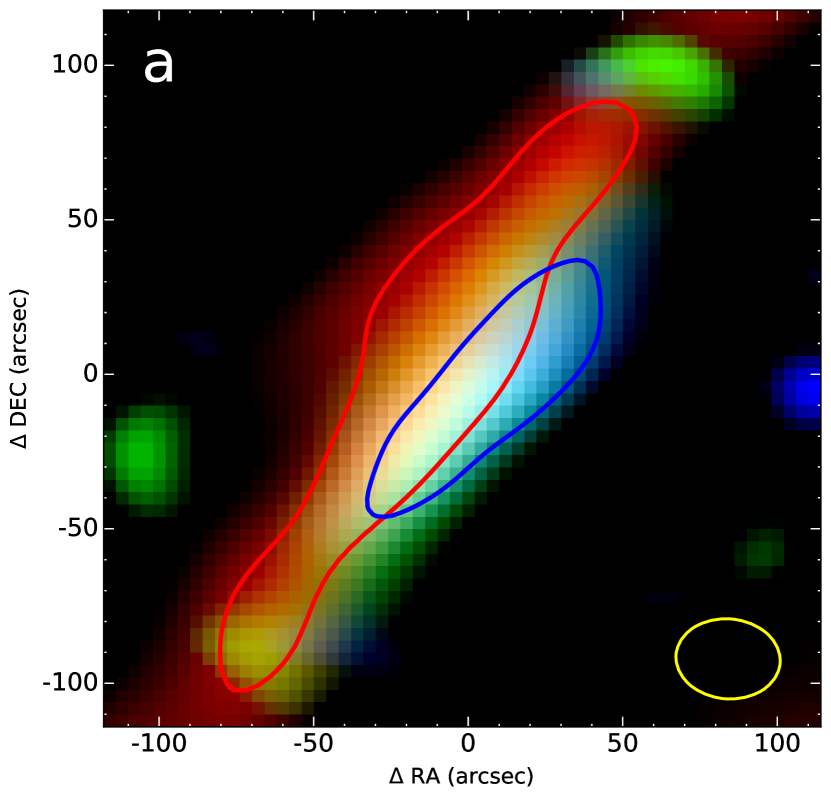
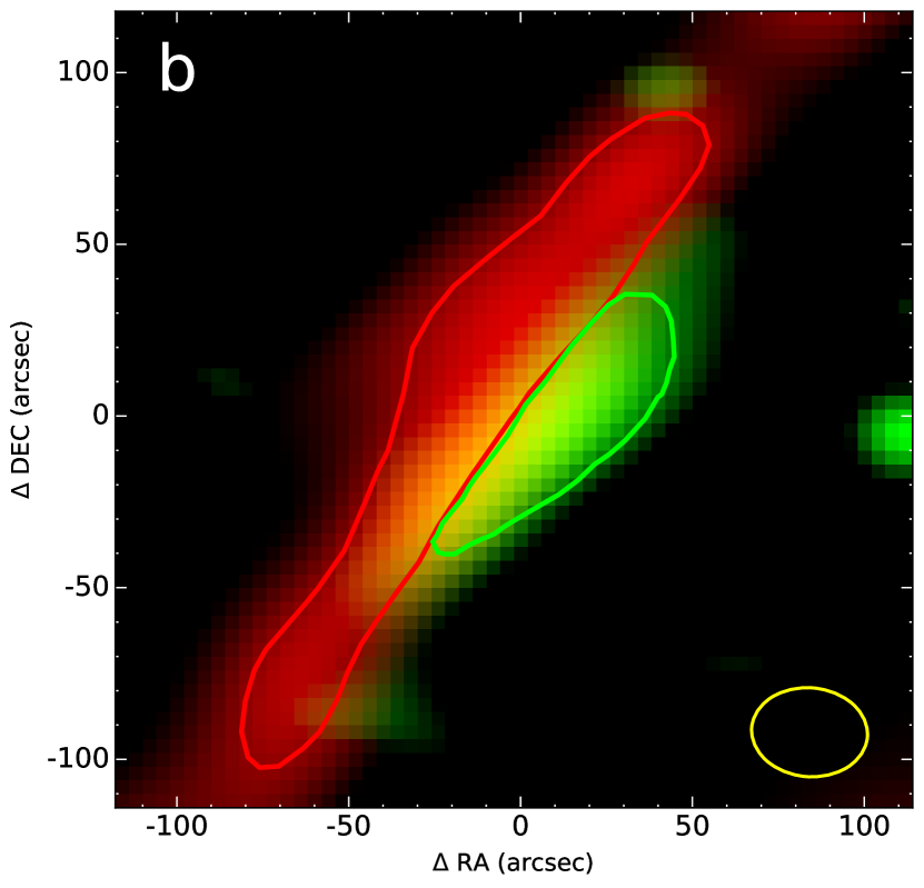
Figure 3: The $\rho$ Oph W filament shifts towards the exciting star with increasing frequency, as illustrated in these colour-coded versions of the restored maps shown in Fig. 1, after subtraction of the SR 4 point source at 39 GHz, and degraded to a common angular resolution. a: This RGB image is linearly scaled to cover the whole range of intensities at each frequency: 17 GHz in red and 33 GHz in green and 39 GHz in blue. The contours are taken at 90% peak intensity, with matching colours. The common beam corresponds to that of the 17 GHz map, and is indicated by the yellow ellipse (see Table 1). b: In this Red-Green version, with 17 GHz in red and 39 GHz in green, we illustrate the photometric apertures used to measure the SED (Sec. 3.2). The contours correspond to the 85%-peak level at 17 GHz (in red), and 80% at 39 GHz, (in green), but are modified to avoid overlap.

We conclude that the cm-wavelength signal from the $\rho$ Oph W filament shifts towards higher frequencies with decreasing distance to the exciting star HD 147889. In other words, these morphological trends with frequency point at spectral variations in the EME spectrum when emerging from the PDR towards the UV source. It is interesting to note that a similar spectral trend has been reported in the PDR surrounding the $\lambda$ Ori region, where the EME signal peaks at increasingly higher frequencies towards the UV source (Cepeda-Arroita et al., 2020). The next Section addresses how the spectral trends implicit in the morphological trends observed in $\rho$ Oph W could be related to varying physical conditions under the spinning dust hypothesis.

3.2 Spectral energy distribution

The multi-frequency radio maps of $\rho$ Oph W allow for estimates of its SED between 5 and 39 GHz. The morphological trends in frequency should be reflected in variations of the SED between the emission originating around the 17 GHz peak and the emission coming from the vicinity of the 39 GHz peak. Such multi-frequency analysis requires smoothing the data to a common beam, which is that of the coarsest observations, at 17 GHz. Once smoothed, we measured the mean intensity in each map inside the two masks shown in Fig. 3. Interferometer data are known to be affected by flux-loss, i.e. missing flux from large angular scales not sampled by the $uv-$coverage of the interferometer. By using a prior image not affected by flux-loss, i.e. as defined in Appendix A, the skymem algorithm allows to recover such flux loss under the assumption of linear correlation with the prior. Our simulations using the prior image recovered the missing flux exactly, but since the cm-wavelength signal does not exactly follow the prior, biases in the flux-loss correction scheme may affect the SEDs reported here. We expect such biases to be small and include them in the absolute calibration error of 10%, given the tight correlation with the near-IR tracers and especially with the IRAC 8 $\mu$m image used to build the prior image.

Table 3 lists the mean intensities $\langle I_{\nu}\rangle$ measured within the 17 and 39 GHz masks, $\mathcal{M}_{17}$ and $\mathcal{M}_{39}$, for the six frequencies that we observed. We weighted the photometric extraction using the noise image $\sigma_{R}(\vec{x})$ given in Eq. 16, i.e.

$$\langle I^{k}_{\nu}\rangle=\frac{\sum_{\vec{x}_{j}\in\mathcal{M}_{k}}w_{R}(\vec{x}_{j})I_{\nu}(\vec{x}_{j})}{\sum_{\vec{x}_{j}\in\mathcal{M}_{k}}w_{R}(\vec{x}_{j})},$$ (3)

for each mask $\mathcal{M}_{k}$, and with $w_{R}=1/\sigma^{2}_{R}$. The associated error is

$$\sigma(I^{k}_{\nu})=\sqrt{\frac{N_{\rm beam}}{\sum_{\vec{x}_{j}\in\mathcal{M}_{k}}w_{R}(\vec{x}_{j})}},$$ (4)

where $N_{\rm beam}$ is the number of pixels in a beam. The same SEDs are also plotted in Fig. 4, where we have included a conservative 10% systematic uncertainty.

When including the 10% absolute flux calibration uncertainty, the difference between the SEDs extracted in the two photometric apertures is not significant. The $\chi^{2}$ distribution yields that the two SEDs are different at 75% confidence. Only the 39 GHz average intensities appear to differ at the 95% confidence level, or 2$\sigma$. Table 3 nonetheless lists the ratio between the measured intensities in each region I${}^{39}_{\nu}/$I${}^{17}_{\nu}$, as this ratio systematically increases with frequency, which may reflect the morphological trends. In Fig. 4, the spectra of the two regions show a steep drop after reaching the peak, at a frequency of $\sim 30$ GHz. We can notice that the difference in measured intensity between the two regions is largest at 39 GHz. The emission from the 39 GHz mask shows a spectrum brighter at higher frequencies than the emission coming from the 17 GHz mask. This is interesting as the 39 GHz mask is shifted towards the direction of the illuminating star HD 147889.

Table 3: ATCA mean intensities and their ratio measured in two masks shown in Fig. 3. The quoted uncertainties refer to the thermal errors only - the actual uncertainties should include 10% in quadrature, and have been applied to the ratio $\rm{I}^{39}_{\nu}/\rm{I}^{17}_{\nu}$.

Frequency	17 GHz mask	39 GHz mask	Ratio
[GHz]	[$\times 10^{4}$ Jy/sr]	[$\times 10^{4}$ Jy/sr]	$\rm{I}^{39}_{\nu}/\rm{I}^{17}_{\nu}$
5.5	$<0.3^{a}$	$<0.3^{a}$	$-$
8.8	$1.83\pm 0.04$	$1.69\pm 0.07$	$0.9\pm 0.1$
17.5	$22.93\pm 0.03$	$20.04\pm 0.04$	$0.9\pm 0.1$
20.2	$43.79\pm 0.06$	$39.99\pm 0.08$	$0.9\pm 0.1$
33.2	$37.32\pm 0.13$	$40.52\pm 0.19$	$1.1\pm 0.1$
39.2	$18.05\pm 0.08$	$23.99\pm 0.11$	$1.3\pm 0.2$

${}^{a}3\sigma$ upper limits using the dispersion of residuals.

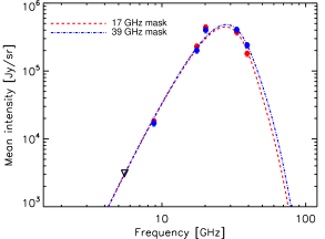
Figure 4: SED of the $\rho$ Oph W filament measured between 5.5 and 39 GHz within the two apertures shown in Fig. 3. The red and blue lines correspond to the best fit spinning dust models.

3.2.1 SED modeling

Previous works have shown that the cm-wave emission from this region is dominated by EME and does not have major contributions from synchrotron or free-free emission, and that its SED on degree angular scales is adequately fit by spinning-dust models (see e.g. Casassus et al., 2008; Planck Collaboration et al., 2011; Arce-Tord et al., 2020). Here we ask the question of what are the consequences of the SED that we measure with ATCA, on arc-minute scales, for the physical conditions and grain populations within the cloud, and under the spinning-dust hypothesis. Since the ATCA mosaic of $\rho$ Oph W is clear of any detectable free-free emission, as shown by the 5 GHz map, we used only a spinning dust component, as calculated using the SPDUST code (Ali-Haïmoud et al., 2009).

The spinning dust emission depends on a large ($\sim$ 10) number of parameters that determine environmental properties: the gas density (n_H), the gas temperature (T), the intensity of the radiation field (parameterised in terms of the starlight intensity relative to the average starlight background, $\chi$), the ionized hydrogen fractional abundance $x_{\rm{H}}\equiv n_{\rm{H^{+}}}/n_{\rm{H}}$, the ionized carbon fractional abundance $x_{\rm{C}}\equiv n_{\rm{C^{+}}}/n_{\rm{H}}$. In addition, the spinning dust emissivities also depend on the grain micro-physics, such as the grain size distribution and the average dipole moment per atom for the dust grains. We will assume that the emission detected by ATCA is originated by spinning PAHs. The motivation for this assumption is the excellent correlation between the radio emission and the 8 $\mu$m map in this region (Casassus et al., 2008; Arce-Tord et al., 2020).

In order to fit the ATCA data using the SPDUST code, we fixed some of the parameters that are well constrained in the literature for this region. Habart et al. (2003) modeled the mid-IR line emission using a PDR code and derived physical parameters for the $\rho$ Oph W filament. Using their results, we fixed the gas temperature and the intensity of the radiation field. For the ionized Hydrogen and Carbon abundances, we took the idealized values for PDRs that are listed in Draine & Lazarian (1998b). We then fitted the SEDs using only 3 free parameters: gas density (n_H), average dipole ($\beta$) and an additional parameter of the grain size distribution ($a_{\rm cutoff}$) that represents the minimum PAH size that is present in the region. This last parameter is necessary to avoid shifting the spinning dust peak to frequencies higher than $\sim 30$ GHz, as predicted by spinning dust models for an ISM dust distribution in dense conditions such as in this PDR. We note that some of the parameters in SPDUST are expected to be highly correlated, for example the gas density, temperature and radiation field. We avoid these degeneracies by fixing most of the parameters to the physical conditions already inferred for this region.

In SPDUST, the grain size distribution is parameterised as in Weingartner & Draine (2001), where the contribution from PAHs is characterized by two log-normal distributions. A typical curve using standard parameters for the Milky Way is shown in black in Fig. 5. We introduced the $a_{\rm cutoff}$ parameter in order to adjust the region of the grain size distribution that is most relevant to the spinning dust emission: the population of the smallest grains. This additional parameter $a_{\rm cutoff}$ corresponds to a characteristic size below which we apply an exponential cutoff modulating the size distribution, so effectively defining a minimum size for the PAHs.

The data in the SEDs were fitted using the IDL routine mpfitfun (Markwardt, 2009), that uses the Levenberg-Marquardt least-squares fit to a function. We performed the fit using the SPDUST model for the two regions shown in Fig. 3. The result from this initial fit gave very similar values between the two regions for $n_{\rm H}$ ($3.0\pm 1.5$ vs $3.1\pm 2.7$) and $\beta$ ($38.7\pm 5.9$ vs $35.1\pm 8.4$). We thus decided to fix $n_{\rm H}$ and $\beta$ and only fit for $a_{\rm cutoff}$. Fig. 4 compares the best fit SPDUST2 model curves with the SED data points.

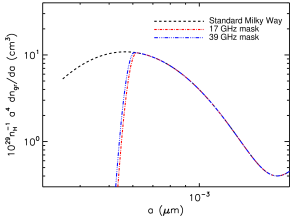
Figure 5: Grain size distribution for sizes around 1 nm for 3 cases. In black is the prescription from Weingartner & Draine (2001) for typical Milky Way parameters. In red and blue are the distributions arising from the spinning dust fit in the two studied regions. In these cases, a cutoff is needed in order to fit the SEDs in Fig. 4.

The result of our fits are summarised in Table 4. The key parameter to account for the observed maximum at 30 GHz is $a_{\rm cutoff}$, without which the peak would shift towards $\sim$90 GHz if fixing the physical conditions to those determined independently in this PDR by Habart et al. (2003). The difference in the free parameter, $a_{\rm cutoff}$, between the two regions is only 1.8 $\sigma$ but it seems to go in the direction expected in a PDR. The minimum grain size $a_{\rm cutoff}$ is slightly larger in the fit of the 17 GHz mask data. This means that in this region, there is a slightly lower abundance of the smallest grains, compared to the other region. This behaviour is in agreement with intuition, as the 39 GHz mask is more exposed to the radiation from HD 147889, which can result in a larger number of the smallest PAHs due to the fragmentation of larger ones. This provides a possible interpretation for the strong morphological differences with frequency, which is reflected in the local SEDs. Vidal et al. (2020) recently concluded that variations in the grain size distribution are also needed to explain spinning dust morphology in the translucent cloud LDN 1780.

The difference in $a_{\rm cutoff}$ between the two regions used to link the multi-frequency morphological variations with spectral trends may seem small. However, it is consistent with equipartition of rotational energy (e.g. Eq. 13 and Eq. 2 in Draine & Lazarian, 1998b; Dickinson et al., 2018, respectively), which suggests that a reduction in grain size from 6.3 nm to 6.0 nm would shift equipartition rotation frequencies $\tilde{\nu}$ from 30 GHz to 31.5 GHz. The spectrum will be shifted accordingly, since for a Boltzmann distribution of rotation frequencies, the emergent emissivity $j_{\nu}/n_{H}$ is modulated by a high frequency Boltzmann cutoff $\exp\left[-\frac{3}{2}\nu^{2}/\tilde{\nu}^{2}\right]$ (see Eq. 63 in Draine & Lazarian, 1998b).

Most of the SPDUST2 parameters were kept fixed in the optimization summarised in Table 4. Yet some of these parameters are expected to vary with depth into the PDR, and most particularly the radiation field. Variations in $\chi$ may also play a role in the spectral variations between the two SED extractions. We tested for the impact of such variations by optimizing a model for the SED in the 17 GHz mask in which we decreased the UV field from our default value of $\chi$=400, to $\chi=100$. The result was a slightly better fit, with reduced $\chi^{2}_{r}=1.5$, and $a_{\rm{cutoff}}=6.2\pm 0.5$Å. Therefore, even with a $\times$4 variation in the intensity of the UV field, an increasing $a_{\rm{cutoff}}$ deeper into the PDR seems to be a robust prediction of the SPDUST2 models.

Table 4: SPDUST2 fit parameters. Parameters without uncertainty were fixed to the ones reported in Habart et al. (2003).

Parameter	Mask${}_{\rm{17\,GHz}}$	Mask${}_{\rm{39\,GHz}}$
$n_{\rm{H}}$ [103 cm-3]	3.2
T [K]	300.0
$\chi$	400.0
$x_{\rm{H}}\equiv n_{\rm{H^{+}}}/n_{\rm{H}}$ [ppm]	1200.0
$x_{\rm{C}}\equiv n_{\rm{C^{+}}}/n_{\rm{H}}$ [ppm]	300.0
$y\equiv 2n(\rm{H_{2}})/n_{\rm{H}}$	0.0
$\beta$	35.2
acutoff [Å]	$6.17\pm 0.04$	$6.07\pm 0.04$
$\chi^{2}_{r}$	2.9	2.4

Further support for an increasing PAH size deeper into the PDR can be found in a comparison with the WISE bands centred on 12 $\mu$m and 3.4$\mu$m, which each correspond to PAH bands and whose ratio is a proxy for PAH size (Allamandola et al., 1985; Ricca et al., 2012; Croiset et al., 2016). The relatively coarse angular resolution of the WISE images (6.1″at 3.4$\mu$m and 15″at 12$\mu$m), compared to IRAC 8$\mu$m (2.5″), prevents their filtering for the ATCA+skymem response. But we can nonetheless degrade the WISE images to the coarsest ATCA beam (at 17 GHz) for a multi-frequency comparison. The smoothed images are not exactly comparable to the ATCA mosaics, since we have not filtered for the ATCA response. But we hope that any resulting bias in the following analysis is small, since our synthesis imaging strategy corrects for missing ATCA antenna spacings using a prior image in skymem, and the main source of PSF sidelobes is due to flux loss from missing antenna spacings at the center of the $uv$-plane. We used the WISE images postprocessed as in (Arce-Tord et al., 2020) to produce Fig. 6, which illustrates that the gradient in peak frequency across the filament is coincident with an increasing WISE 12 $\mu$m/3.4$\mu$m ratio. We quantify this trend using a standard Pearson correlation test $r$ (e.g. same as $r_{\rm sky}$ in Eq. 11 of Arce-Tord et al., 2020), so similar to $r_{w}$ in Eq. 2 but without the weights, and instead adjusting the field of extraction to avoid the noise at the edge of the ATCA mosaics. The resulting Pearson $r$ are listed in Table 5. We recover the same trend as in Table 2, both $r$ and $r_{w}$ point at 20 GHz as the best match to IRAC 8$\mu$m. However, the ATCA map that best traces the shorter WISE wavelength is 39 GHz. The excellent correlation between ATCA 33/39 GHz with 3.4 $\mu$m and also between ATCA 20/17 GHz with the 8 $\mu$m template confirm the strong correlation between AME and PAH emission in this region.

The AME-PAH connection was put in doubt by Hensley et al. (2016) based on a full-sky analysis on angular scales of 1 deg. Indeed, when taken as a whole, the $\rho$ Oph cloud is a good example of the breakdown of the correlation between PAHs tracers and AME, since S 1, the brightest nebula in the complex in IRAC 8$\mu$m and also in Spitzer-IRS 11.3$\mu$m PAH band (Casassus et al., 2008, their Table 2), has no detectable EME signal. However, it appears that EME and PAHs do correlate very tightly in higher angular resolution observations, and in regions where EME is present. Another example of excellent correspondence between AME and PAH emission is shown clearly in LDN1246 (Scaife et al., 2010).

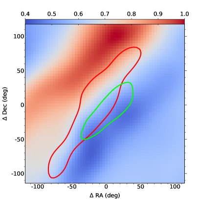
Figure 6: Comparison between the ATCA continuum and a proxy for PAH size. We show an overlay of a 17 GHz contour (in red, at 85%-peak) and a 39 GHz contour (in green, at 80%-peak), on the ratio of WISE 12$\mu$m to 3.4$\mu$m. The increasing value of the ratio deeper into the PDR is consistent with the larger PAHs.

The predictions for the grain-size distribution reported here should also be compared to the IR spectra available for $\rho$ Oph W. Under the spinning dust hypothesis for EME, a complete model should reproduce simultaneously the radio SED as well as the IR spectra, which are both due to the same underlying dust population. Here we limit the scope of this report on the new ATCA observations to only the radio part, highlighting the need for a future modeling effort.

Table 5: ATCA - WISE correlation statistics

Frequency	WISE 3.4$\mu$m	IRAC 8$\mu$m
MHz
17481	0.01a	0.82
20160	0.24	0.90
33157	0.91	0.68
39157	0.93	0.44

^a Pearson $r$ coefficients. All values bear a 1$\sigma$ uncertainty of 0.04.

4 Carbon RRL search

The main spin-up mechanisms that could lead to VSG rotation frequencies of up to $\sim$30 GHz may be either radiative torques or plasma drag (Draine & Lazarian, 1998b). Interestingly, the brightest near-IR nebulae in $\rho$ Oph, i.e. S 1 and SR 3, have no radio counterparts at cm-wavelengths. Yet the circumstellar environments of embedded early-type stars correspond to the highest UV-radiation intensities. The absence of radio sources coincident with the IR-bright circumstellar dust about S 1 and SR 3 cannot be reconciled with VSG depletion, as marginally shown by the CBI observations reported by Casassus et al. (2008), and confirmed with CBI2 in Arce-Tord et al. (2020). Radiative torques seem unlikely to explain the strong radio signal from the $\rho$ Oph W filament.

The alternative source of rotational excitation, plasma drag, is due to the interaction of the grain dipoles with passing ions - namely H⁺ or C⁺ in the context of PDRs. If so the spinning dust emissivities would be best understood in terms of an emission measure: $I_{\mathrm{cm}}\propto N_{\mathrm{VSG}}N(\mathrm{C}+)$. An observational test of the plasma-drag hypothesis requires measurements of the C⁺ abundance, as can be inferred using radio carbon recombination lines. The faint or absent cm-wavelength signal from the circumstellar nebulae around S 1 and SR 3 in the radio maps may be due to these stars being too cold to create conspicuous C ii regions (Casassus et al., 2008).

Pankonin & Walmsley (1978) examined the most complete set of RRL data towards $\rho$ Oph to date. The line profiles observed at lower frequencies have widths of 1.5 km s^-1 FWHM. They mapped the neighbourhood of S 1, but did not extend their coverage to $\rho$ Oph W, unfortunately. The highest frequency RRLs considered by Pankonin & Walmsley (1978) are C90$\alpha$ and C91$\alpha$, at $\sim$9 GHz, which they interpreted as stemming from circumstellar gas about S 1, with electron densities $n_{\rm e}\sim 15\,$cm^-3 and $T_{\rm e}\sim 150\,$K. This circumstellar C ii region was inferred to be less than $\sim$2 arcmin in diameter, and surrounded by a diffuse halo with $n_{\rm e}\sim 1\,$cm^-3, traced by the lower frequency carbon RRLs.

We searched for carbon RRLs in the ATCA+CABB data, with a 2 GHz bandwidth centred on 17481 MHz. Three $\alpha$-type RRLs fall into the 17481 GHz IF: C71$\alpha$ 18.00153, C72$\alpha$ 17.26682, C73$\alpha$ 16.57156. No carbon RRLs are detected near the systemic velocity of $\rho$ Oph W (which is $V_{\mathrm{lsr}}=+3\,$km s^-1 Brown & Knapp, 1974; Pankonin & Walmsley, 1978). In the 17481 GHz IF the velocity width of each channel is $\sim$16 km s^-1. The noise in single-channel reconstructions is $\sim$2 mJy beam^-1, for a 30 arcsec beam FWHM. Assuming that the line is unresolved and is diluted in such broad channels, this upper limit is a factor of two looser than that obtained by Casassus et al. (2008) using Mopra.

For a rough estimate of carbon RRL intensities in $\rho$ Oph W, we take a depth of 0.04 pc, which at a distance of 135 pc subtends 1 arcmin, an ionisation fraction of $10^{-4}$, due to carbon photoionisation, $T_{\rm e}=100\,$K, and a H-nucleus density of $n_{\mathrm{H}}=10^{5}$ cm^-3 (these values are similar to those reported previously for $\rho$ Oph W, e.g. Habart et al., 2003). The peak intensity of the emergent C71$\alpha$ is 18 mJy beam^-1, for LTE, with a 1.5 km s^-1 FWHM, and a 30 arcsec beam. When diluted in the $\sim$ 16 km s^-1 channels of CABB, the expected signal drops down to $\sim$ 1 mJy beam^-1, or close to the limits obtained with Mopra. However, the expected CRRLs intensities should be within easy reach with the Atacama Large Millimetre Array (ALMA), as long as the spectral resolution is not degraded much beyond $\sim$0.5 km s^-1. The spectra line data could be acquired as part of future observations to map the EME signal in $\rho$ Oph W at $\sim$40 GHz with the Band 1 receivers currently under construction, and which should yield a noise level of 3 mJy beam^-1 in 40 min and in 0.5 km s^-1 channels.

5 Conclusion

ATCA+CABB multi-configuration mosaics of the $\rho$ Oph W PDR resolve the filament with $\sim$30 arcsec resolutions from 5 GHz to 39 GHz. Since the signal fills the primary beam a special purpose imaging synthesis strategy (skymem) was applied to compensate for flux loss and mitigate sidelobe oscillations with the incorporation of an image prior.

The multi-frequency 17 GHz to 39 GHz mosaics reveal spectral variations within $\rho$ Oph W. The radio signal follows the near-IR filament, but it is progressively shifted towards the UV source at higher frequencies. Such morphological differences in frequency reflect changes in the radio spectrum as a function of position in the sky. While the morphological trends with frequency are qualitative, the corresponding spectral variations in terms of the SEDs are not significant given the systematic uncertainties.

The SED of $\rho$ Oph W, with a very narrow peak at $\sim$30 GHz, is reminiscent of spinning-dust. The physical conditions inferred under this hypothesis, using an optimization of selected free-parameters in the SPDUST package, are consistent with those derived in the literature, but require a minimum grain size cutoff and relatively large electric dipoles. The cutoff in the grain sizes is particularly well constrained as a standard ISM size distribution would shift the peak of the spectrum towards $\sim$90 GHz. The spinning dust model accounts for the measured intensities, and suggests that the qualitative morphological differences can be interpreted in terms of an increasing minimum grain size deeper into the PDR.

Further sampling of the spinning dust spectrum in $\rho$ Oph W at $\sim$50GHz with ALMA, in the context of the data reported here, would provide strong constraints on the minimum PAH size. Eventually, the predictions obtained from the rotational emission of PAHs should be tested against a physical model for the IR PAH bands in $\rho$ Oph W.

Data Availability

The skymem package can be found at https://github.com/simoncasassus/SkyMEM. The corresponding author will provide help to researchers interested in porting skymem to other applications. The skymem code repository also includes, as an example application, the sky-plane version of the data underlying this article. The unprocessed visibility dataset can be downloaded from the Australia Telescope Online Archive at https://atoa.atnf.csiro.au/. The corresponding author will share the calibrated visibility data on reasonable request.

Appendix A Image reconstruction

The traditional image-reconstruction algorithm Clean is not ideal for extended sources that fill the beam, especially with sparse $uv$-coverage. Initial trials at imaging using the Miriad task ‘clean’ resulted in large residuals, with an intensity amplitude much greater than that expected from thermal noise, and with a spatial structure reflecting the convolution of the negative synthetic side-lobes with the morphology of the source (see Fig. 7). Attempts to improve dynamic range using the ‘maxen’ task in Miriad gave worse results. We therefore designed a special-purpose image reconstruction algorithm, based on sky-plane deconvolution (hereafter skymem), and that allows the incorporation of priors to recover the larger angular scales.

The present sky-plane approach is an alternative to similar non-parametric imaging synthesis strategies based on a $uv$-plane approach, in which model visibilities are compared to the interferometer data. An example package for such $uv$-plane approaches is uvmem (Casassus et al., 2006; Cárcamo et al., 2018), which has been applied to diffuse ISM data (such as the CBI and CBI2 observations of $\rho$ Oph, Casassus et al., 2008; Arce-Tord et al., 2020) as well as in compact sources (e.g. such as VLA and ALMA observations of protoplanetary discs Casassus et al., 2018, 2019; Pérez et al., 2019). Both the sky-plane and the $uv$-plane approaches should of course be equivalent, but in the sky plane we avoid delicate issues with visibility gridding. In this application of skymem we rely entirely on the Miriad gridding machinery.

In a sky-plane formulation of image synthesis, the data correspond to the dirty maps $\{I^{D}_{j}\}_{j=1}^{f}$ for each of the $f$ fields in the mosaic. In order to obtain a model sky image that fits the data we need to solve the usual deconvolution problem, i.e. obtain the model image $I^{m}$ that minimizes a merit function $\mathcal{L}$:

$$\mathcal{L}=\chi^{2}-\lambda\mathcal{S}(I^{m}),$$ (5)

where

$$\chi^{2}=\sum_{j=1}^{f}\sum_{i=1}^{n}w_{j}(\vec{x}_{i})\left(I^{D}_{i}(\vec{x}_{i})-I^{Dm}_{j}(\vec{x}_{i})\right)^{2}.$$ (6)

The sums extend over the number of fields, $f$, and over the number of pixels in the model image, $n$. Each of the model dirty maps, $I^{Dm}_{j}$, correspond to the convolution of the attenuated $I^{m}$ with the synthetic beam $B_{j}$,

$$I^{Dm}_{j}=(I^{m}_{j}A_{j})\ast B_{j},$$ (7)

where $\{A_{j}\}_{j=1}^{f}$ are the primary beam attenuations for all fields. The weight map for a field $j$ is given by $w_{j}=1/\bar{\sigma}_{j}^{2}$, where $\bar{\sigma}_{j}$ is the theoretical noise map as calculated with the ‘sensitivity’ option to the task ‘invert’ in Miriad. This noise map is simply the thermal noise expected in the dirty map divided by the primary beam attenuation.

After several trials with a variety of functional forms for $\mathcal{S}$, we found that we obtained best results by simply using $\lambda=0$, i.e. with pure $\chi^{2}$ reconstructions. Image positivity of its own provided enough regularization. We used the Perl Data Language (PDL) for high-level data processing, and the optimization was carried out with a PDL-C patch to the Fletcher-Reeves algorithm in its GSL implementation. We enforced positivity by clipping $I^{m}>0$ at each evaluation of $\mathcal{L}$ and its gradient. A couple of aspects of the implementation of skymem are worth mentioning. In the convolution of Eq. 7 the kernel should not be normalized, as would be the case for smoothing. Instead, to yield $I^{Dm}_{j}$ in Jy beam^-1 units, $B_{j}$ should be scaled by the number of pixels in a beam $\Omega_{G}/(\delta x)^{2}$, where $\Omega_{G}$ is the clean beam solid angle (see below) and $\delta x$ is the pixel scale. Another relevant aspect is the evaluation of the gradient of $\chi^{2}$, which can be written

$$\frac{\partial\chi^{2}}{\partial I^{m}(\vec{x}_{i})}=\sum_{j=1}^{f}\frac{2A_{j}(\vec{x}_{i})}{\bar{\sigma}^{2}}\left[\left(I^{Dm}-I^{D}\right)\ast B_{j}\right]_{\vec{x}_{i}}.$$ (8)

The initial condition is important for the optimization as its parameter space is very structured. A blank initial image performed better that Clean, but yet lower values of $\mathcal{L}$ were obtained by starting with an image known to approximate the radio signal, which we call the prior image. The initial image we chose is the IRAC 8$\mu$m map, in its original angular resolution but filtered for point sources. This version of the IRAC 8$\mu$m map was multiplied by a representative dimensionless radio/IR correlation slope of $5.2\times 10^{-4}$ (extrapolated from the slopes reported in Castellanos et al., 2011), so that the flux densities fall within the order of magnitude of the observed CBI flux densities in such sources. We then refined the intensity scale to exactly match that of the the ATCA observations in the following way. We simulated ATCA observation on the IRAC 8 $\mu$m template, with identical $uv$-plane coverage as the observations, and calculated the dirty maps $\{I^{D}_{\mathrm{IRAC}j}\}_{j=1}^{f}$ for each pointing $j$ in these mock data. The best fit correlation slopes $\{s_{j}\}_{j=1}^{f}$, defined by $I^{D}_{j}=s_{j}I^{D}_{\mathrm{IRAC}j}$, are each given by

$$s_{j}=\frac{\sum_{i}w_{j}(\vec{x}_{i})I^{D}_{\mathrm{IRAC}j}(\vec{x}_{i})I^{D}_{j}(\vec{x}_{i})}{\sum_{i}w_{j}(\vec{x}_{i})(I^{D}_{\mathrm{IRAC}j}(\vec{x}_{i}))^{2}}.$$ (9)

Finally, the prior image corresponds to this IRAC 8 $\mu$m template scaled by $\langle s\rangle$, the mean correlation slope taken over all pointings. These prior images and their associated intensity scales are shown in Fig. 7. Table 6 lists the values for $\langle s\rangle$ and $\sigma(s)$ at each frequency. It is interesting to compare with the radio-IR correlation slopes $a(\nu)$ listed in Table 2. The larger dispersion of $s(\nu)$ with increasing frequency could reflect either real spectral changes. For the skymem simulations on the IRAC template, all $s(\nu)\equiv 1$ .

Table 6: Scale factors for the skymem priors

Frequencya	$\langle s\rangle^{b}$	$\sigma(s)\,^{c}$
5500	0.015	-
8800	0.114	-
17481	1.694	0.163
20160	3.162	0.269
33157	2.495	0.546
39157	1.090	1.021

^a Centre frequency in MHz. ^b Average and ^c dispersion taken over all pointings.

The resulting model images are shown in Fig. 7. It can be appreciated that the free parameters in the model image are modified relative to the input prior only within the field of the ATCA mosaic. It is also interesting to note that the low spatial frequencies of the prior are preserved, since the ATCA data provide no information that would constrain them.

Image restoration was obtained by smoothing the model image with the clean beam $G$ in a reference field (that also sets the Jy beam^-1 units), and by adding the linear mosaic of dirty residuals $R^{D}$,

$$I^{R}=I^{m}\ast G+R^{D}.$$ (10)

The residual image for each pointing $j$ is $T^{D}_{j}=I^{D}_{j}-I^{Dm}_{j}$, so

$$R^{D}=\frac{\sum_{j}w_{j}T^{D}_{j}A_{j}}{\sum_{j}w_{j}A_{j}^{2}}.$$ (11)

The residual and restored images are shown in Fig. 7. The residuals are adequately thermal, but the linear mosaic generated with the formula in Eq. 11 amplifies the noise at the edges of the field. Thus we also provide in Fig. 7 a version of each restored images after multiplication by the mosaic attenuation pattern $\mathcal{A}$ to highlight the regions with smallest thermal errors, with

$$\mathcal{A}(\vec{x})=\frac{\bar{\sigma}_{\circ}}{\bar{\sigma}_{R}(\vec{x})},$$ (12)

where $\bar{\sigma}_{\circ}$ is the minimum value in the theoretical noise image,

$$\bar{\sigma}_{R}=\sqrt{\frac{1}{\sum_{j}w_{j}A_{j}^{2}}}.$$ (13)

The dynamic range of the resulting skymem images can be estimated by calculating the mean and dispersion of the residuals, i.e.

$$\langle R^{D}\rangle=\frac{\sum_{j}\bar{w}_{R}(\vec{x}_{j})R^{D}(\vec{x}_{j})}{\sum_{j}\bar{w}_{R}(\vec{x}_{j})},$$ (14)

and

$$\sigma_{\circ}=\sqrt{\frac{\sum_{j}\bar{w}_{R}(\vec{x}_{j})\left(R^{D}(\vec{x}_{j})-\langle R^{D}\rangle\right)^{2}}{\sum_{j}\bar{w}_{R}(\vec{x}_{j})}}.$$ (15)

The values for $\sigma_{\circ}$ are given in Table 7, where we see that they come close to the theoretical ATCA sensitivity. The noise image measured using the residuals rather than the theoretical sensitivy can be written as

$$\sigma_{R}=\sigma_{\circ}\frac{\bar{\sigma}_{R}}{\bar{\sigma}_{\circ}}.$$ (16)

Table 7: Dispersion of residuals and expected theoretical noise, in $\mu$Jy beam^-1

Frequencya	$\sigma_{\circ}^{b}$	$\sigma_{\rm ETC}^{c}$
5500	24	5
8800	23	6
17481	13	12
20160	25	19
33157	38	17
39157	23	16

^a Centre frequency in MHz. ^b Measured dispersion of skymem residuals. ^c Expected noise level in full scans, from the Exposure Time Calculator at https://www.narrabri.atnf.csiro.au/myatca/interactive_senscalc.html.

Figure 7: Synthesis imaging of the ATCA observations of $\rho$ Oph W. $x-$ and $y-$ axis correspond to offset R.A. and Dec. in arcmin. This panel of images is organized as a table, where each image corresponds to the frequency given in column headers, for the synthesis imaging schemes given in line headers. We have, from top to bottom, the dirty and clean mosaics calculated with Miriad, the prior image scaled to each frequency, followed by the skymem model image, its associated residual mosaic, and the restored mosaic, shown also also after multiplication by the mosaic attenuation (labeled ‘skymem restored PB’). The beam ellipses are shown in the restored images. The colour units are mJy beam^-1. These images have not been point-source subtracted.

References

- Ali-Haïmoud (2014) Ali-Haïmoud Y., 2014, MNRAS, 437, 2728
- Ali-Haïmoud et al. (2009) Ali-Haïmoud Y., Hirata C. M., Dickinson C., 2009, Monthly Notices of the Royal Astronomical Society, 395, 1055
- Allamandola et al. (1985) Allamandola L. J., Tielens A. G. G. M., Barker J. R., 1985, ApJ, 290, L25
- Arce-Tord et al. (2020) Arce-Tord C., et al., 2020, MNRAS, 495, 3482
- Brown & Knapp (1974) Brown R. L., Knapp G. R., 1974, ApJ, 189, 253
- Cárcamo et al. (2018) Cárcamo M., Román P. E., Casassus S., Moral V., Rannou F. R., 2018, Astronomy and Computing, 22, 16
- Casassus et al. (2006) Casassus S., Cabrera G. F., Förster F., Pearson T. J., Readhead A. C. S., Dickinson C., 2006, ApJ, 639, 951
- Casassus et al. (2008) Casassus S., et al., 2008, MNRAS, 391, 1075
- Casassus et al. (2018) Casassus S., et al., 2018, MNRAS, 477, 5104
- Casassus et al. (2019) Casassus S., et al., 2019, MNRAS, 483, 3278
- Castellanos et al. (2011) Castellanos P., et al., 2011, MNRAS, 411, 1137
- Cepeda-Arroita et al. (2020) Cepeda-Arroita R., et al., 2020, arXiv e-prints, p. arXiv:2001.07159
- Cieza et al. (2019) Cieza L. A., et al., 2019, MNRAS, 482, 698
- Croiset et al. (2016) Croiset B. A., Candian A., Berné O., Tielens A. G. G. M., 2016, A&A, 590, A26
- Davies et al. (2006) Davies R. D., Dickinson C., Banday A. J., Jaffe T. R., Górski K. M., Davis R. J., 2006, MNRAS, 370, 1125
- Dickinson et al. (2018) Dickinson C., et al., 2018, New Astron. Rev., 80, 1
- Draine & Hensley (2012) Draine B. T., Hensley B., 2012, ApJ, 757, 103
- Draine & Lazarian (1998a) Draine B. T., Lazarian A., 1998a, ApJ, 494, L19+
- Draine & Lazarian (1998b) Draine B. T., Lazarian A., 1998b, ApJ, 508, 157
- Draine & Lazarian (1999) Draine B. T., Lazarian A., 1999, ApJ, 512, 740
- Elias (1978) Elias J. H., 1978, ApJ, 224, 453
- Finkbeiner et al. (2002) Finkbeiner D. P., Schlegel D. J., Frank C., Heiles C., 2002, ApJ, 566, 898
- Gaia Collaboration (2018) Gaia Collaboration 2018, VizieR Online Data Catalog, p. I/345
- Garufi et al. (2020) Garufi A., et al., 2020, A&A, 633, A82
- Gold et al. (2011) Gold B., et al., 2011, ApJS, 192, 15
- Habart et al. (2003) Habart E., Boulanger F., Verstraete L., Pineau des Forêts G., Falgarone E., Abergel A., 2003, A&A, 397, 623
- Hensley & Draine (2017) Hensley B. S., Draine B. T., 2017, ApJ, 836, 179
- Hensley et al. (2016) Hensley B. S., Draine B. T., Meisner A. M., 2016, ApJ, 827, 45
- Hoang & Lazarian (2016) Hoang T., Lazarian A., 2016, ApJ, 821, 91
- Hoang et al. (2010) Hoang T., Draine B. T., Lazarian A., 2010, ApJ, 715, 1462
- Hoang et al. (2016) Hoang T., Vinh N.-A., Quynh Lan N., 2016, ApJ, 824, 18
- Högbom (1974) Högbom J. A., 1974, A&AS, 15, 417
- Kogut et al. (1996) Kogut A., Banday A. J., Bennett C. L., Gorski K. M., Hinshaw G., Reach W. T., 1996, ApJ, 460, 1
- Lada & Wilking (1984) Lada C. J., Wilking B. A., 1984, ApJ, 287, 610
- Le Petit et al. (2006) Le Petit F., Nehmé C., Le Bourlot J., Roueff E., 2006, ApJS, 164, 506
- Leitch et al. (1997) Leitch E. M., Readhead A. C. S., Pearson T. J., Myers S. T., 1997, ApJ, 486, L23+
- Liseau et al. (1999) Liseau R., et al., 1999, A&A, 344, 342
- Markwardt (2009) Markwardt C. B., 2009, in Bohlender D. A., Durand D., Dowler P., eds, Astronomical Society of the Pacific Conference Series Vol. 411, Astronomical Data Analysis Software and Systems XVIII. p. 251 (arXiv:0902.2850)