Estimating longterm power spectral densities in AGN from simulations

Abstract

The power spectral density (PSD) represents a key property quantifying the stochastic or random noise type fluctuations in variable sources like Active Galactic Nuclei (AGN). In recent years, estimates of the PSD have been refined by improvements in both, the quality of observed lightcurves and modeling them with simulations. This has aided in quantifying the variability including evaluating the significance of quasi-periodic oscillations. A central assumption in making such estimates is that of weak non-stationarity. This is violated for sources with a power-law PSD index steeper than one as the integral power diverges. As a consequence, estimates of the flux probability density function (PDF) and PSD are interlinked. In general, for evaluating parameters of both properties from lightcurves, one cannot avoid a multi-dimensional, multi-parameter model which is complex and computationally expensive, as well as harder to constrain and interpret. However, if we only wish to compute the PSD index as is often the case, we can use a simpler model. We explore a bending power-law model instead of a simple power-law as input to time-series simulations to test the quality of reconstruction. Examining the longterm variability of the classical blazar Mrk 421, extending to multiple years as is typical of Fermi-LAT or Swift-BAT lightcurves, we find that a transition from pink (PSD index one) to white noise at a characteristic timescale, $t_{b}\sim 500-1000$ years, comparable to the viscous timescale at the disk truncation radius, seems to provide a good model for simulations. This is both a physically motivated as well as a computationally efficient model that can be used to compute the PSD index.

Keywords First keyword  $\cdot$ Second keyword  $\cdot$ More

1 Introduction

A key area of time domain astronomy involves the modeling of noisy time-series or lightcurves. This usually requires the shape of the noise spectrum or the power spectral density (PSD) as input. Several estimation problems of temporal features depend upon the type and level of noise that acts as background. For example, estimation of the significance of quasi-periodic oscillations depends on the assumed level of noise which in turn depends upon the PSD (e.g., Ackermann et al., 2015; Vaughan et al., 2016; Covino et al., 2019; Ait Benkhali et al., 2020). Estimation of variability properties also depends upon the probability distribution function (PDF) from which fluxes are drawn. Indeed, the PDF and the PSD are the two key properties that are central to quantifying statistically, the variability of a source with stochastic processes. They are the primary observables upon which other observables that allow us to probe the physical processes driving variability, depend on. Consequently, they both are also key inputs to simulation methods used to statistically characterise the variability properties. Such simulation techniques are based on spectral density estimation, a fundamental aspect of time domain astrophysics that has seen development at different stages in the last few decades (Timmer and Koenig, 1995; Vaughan, 2013).

In principle, the PDF and the PSD are independent inputs or observables. The PSD represents the distribution of power at different timescales. It carries information about the strength of the physical processes driving variability at particular timescales (e.g., Rieger, 2019, for a recent discussion). Often the functional form of the PSD can be approximated by a power-law that may include a characteristic break separating regions of different indices (e.g., Uttley et al., 2002). The PDF, on the other hand, represents the probability distribution of the flux itself and encodes the form or class of the physical process. For instance, the PDF can discriminate between additive and multiplicative processes depending on whether it is normal or lognormal (Uttley et al., 2005). However, these observables as inputs to simulation both impact on the estimation of variability. And through this degeneracy of effects, they interact with each other. For instance, the estimates of the PSD shape with the Timmer-Koenig (hereafter TK95) method relies on the assumption that the PDF is Gaussian or normal. If it fails, the estimates are no longer reliable as shown in e.g., Vaughan et al. (2003) and Morris et al. (2019). This is because of the divergence of total power leading to weak non-stationarity as explained in e.g., Vaughan et al. (2003) and Uttley et al. (2005).

A variety of PSD analyses have been performed in recent times for the longterm lightcurves of gamma-ray emitting Active Galactic Nuclei (AGN), particularly in the high-energy Fermi-LAT domain. In the majority of cases, the inferred PSDs appear compatible with power laws $P(f)\propto f^{-\Gamma}$ with $\Gamma\sim 0.8-1.6$ (e.g., Abdo et al., 2010; Ackermann et al., 2011; Sobolewska et al., 2014; Max-Moerbeck et al., 2014; H.E.S.S. Collaboration et al., 2017; Kushwaha et al., 2017; Bhatta and Dhital, 2020; Ait Benkhali et al., 2020; Goyal, 2020)

In this paper, we wish to have a revised look at the problem of PSD estimation. Due to the presence of weak non-stationarity for PSD indices steeper than one, we need to find ways to prevent the total power at low frequencies from diverging. One convenient way to do this, is to introduce a break, $f_{\rm break}$ or a bend to transition from coloured noise, appropriate for the observed variations, to white noise that we will eventually be reduced to at long enough timescales. This is because, for any real object the variability power spectra must converge. We cannot have an infinitely large quantity of power in variations at any timescale including the longest ones. While this is, a priori a mathematical technique to avoid divergence, the presence of breaks in the PSD is also motivated physically. Thus, in this paper we explore the mathematical effect of inserting a break or a bend in determining the PSD using simulation, taking multi-year lightcurves of the blazar Mrk 421 as example. We also provide a physical motivation for the presence of breaks, and compare it to those that work for simulations.

Another approach is to try and model accurately the shape of the true PDF. This is certainly a worthy approach and the sophisticated simulation technique in Emmanoulopoulos et al. (2013) would be the framework to adopt (we will refer to it as DE13 henceforth). However, there are at least two challenges. First, as we test more complex models than a simple power-law PSD, we have several free parameters (e.g., four for a broken power-law) and need long lightcurves with a fine cadence to constrain them adequately. Secondly, and perhaps more crucially, approaches like DE13 are computationally very expensive. This makes it rather challenging to adopt these without significant modifications to speed up the algorithms, for detecting and significance testing temporal features in big data sets.

In this study, we focus on the long term variability behaviour and not on short outbursts or flares. We are interested in studying the transition regime(s) at timescales longer than those for fast variability (occurring on scales of minutes). The flares represent sharp and transient changes in variability properties potentially leading to a departure from the underlying distribution or flux probability distribution function (PDF) of the default, persistent mechanism.

From Morris et al. (2019) we know that for power-law PSD indices steeper than pink noise ($\Gamma>1$), there is weak non-stationarity. This affects the time-series simulations in that the PDF does not remain fixed for the entire ensemble. This is true independent of red noise leakage corrections as it has to do with divergence of power at longer timescales. Here we explore a way to address this by introducing a break or a bend in the PSD. The position of this break then becomes crucial and could either come directly from physical models (e.g., viscosity timescale) or in absence of this, from methodologically testing what explains best the observations. In the present paper we use simulated observations of known PSD indices to explore the relation between a physical break and a methodological break. We find that the two converge for long term variations akin to multi-year Fermi-LAT or Swift-BAT lightcurves to within a factor of a few.

The paper is organised as follows. In section 2, we illustrate first with an analytical model and then with a physical model of accretion disk powered fluctuations, the effect of and need for the break in the PSD. This will then be tested with artificial lightcurves generated by the time-series simulations described in the next section 3. Section 4 explains the results of the tests evaluating the position of the break or bend on reconstructing the "true" PSD from observed lightcurves, both using artificially generated power-laws as well as real observations of Mrk 421, a classical blazar at X-ray and gamma-ray energies. In the final section 6, we present a discussion of the results and conclusions.

2 General Considerations

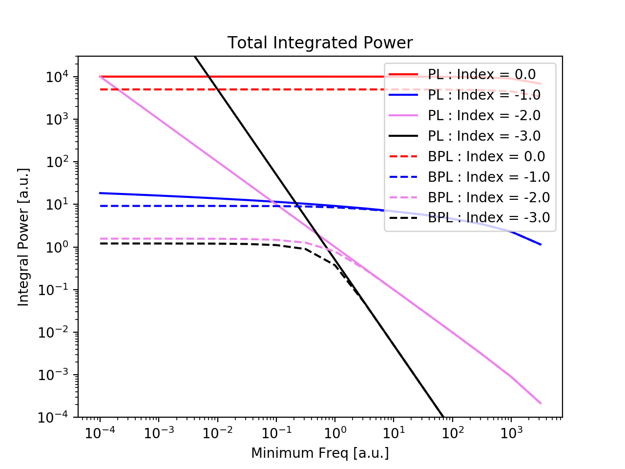
Figure 1: Figure illustrating the difference in total power between extending a power-law model of indices [0,3] and a bending power law with a bend or break frequency at one. Obviously, the effects are stronger for steeper indices. Therefore, the sensitivity to the position of the break $f_{\rm break}$ is also greater for sharper transitions.

As is evidenced by prior endeavours at PSD estimation and its applications (e.g., Vaughan et al., 2003; Uttley et al., 2005; Vaughan, 2013; Morris et al., 2019), there are several effects at play. In order to disentangle some of these effects and build an intuitive understanding, we employ two toy models.

2.1 PSD characterizations

We take simple power law (PL) and broken or bending power law (BPL) models to investigate the power as a function of different parameters like the break frequency, $f_{\rm b}$, the power law index, $\Gamma$, and the minimum frequency, $f_{\rm min}$ which is associated with the longest timescales. The PL and BPL models are formally given by,

$$P(f)=A\ \left(\frac{f}{f_{\rm b}}\right)^{-\Gamma}$$ (1)

and,

$$P(f)=\frac{A}{1+\left(\frac{f}{f_{\rm b}}\right)^{\Gamma}}\,.$$ (2)

For the chosen BPL model the transition from a power-law type shape with index $\Gamma$ to white noise (of index zero) is a smooth one. This is also the mathematical form appropriate for an Ornstein-Uhlenbeck (OU) process which is a popular model for noisy lightcurves in quasars (e.g., Kelly et al., 2009). The OU process has a constant diffusion coefficient and is key to a mathematical description of Brownian and Johnson noise (see Gillespie, 1996, for a review). On the other hand, a simple broken power-law (BrPL) model, as given by

$$P(f) = A\ \ \ \ \ \ \ \ \ \ \ \ \ \ \ \ \ \ (f<f_{\rm b})$$ (3)

$$= A\ \left(\frac{f}{f_{\rm b}}\right)^{-\Gamma}\ \ \ \ \ \ (f\geq f_{\rm b})\,,$$

is less smooth and in that way less physical.

We then evaluate the total power in a given frequency band, $[f_{\rm min},f_{\rm max}]$ as a function of $f_{\rm min}$ for different PL and BPL models. This provides a quantitative understanding of the amount of power below the bend for different values of index $\Gamma$, which can be transferred to higher frequencies above the bend. As shown in figure 1, it is clear that as $f_{\rm min}\rightarrow 0$ the total power converges or asymptotes to a fixed value for the BPL models rather than diverge as for the PL models. This is because the noise properties transition to white noise, and below a certain frequency (or above the equivalent timescale) this white noise dominated regime will not have a significant amount of additional power by extending the bandwidth to lower frequencies.

For a finite bandwidth, naturally the integral power is finite and does not diverge. It is obvious, however, that the difference in total power between each pair of PL and BPL with the same $\Gamma$ increases with steeper indices, and becomes quite significant as we go to indices greater than one. This marked difference is essentially responsible for making the PSD estimation more challenging beyond this value. It also illustrates that the absolute difference in total power depends upon the value of the break frequency. The lower the break frequency, the greater is the power, both differential and integral at longer timescales. As we will see in the subsequent sections, for the simulated ensembles there appears to be an optimal choice for the break frequency that fixes the mathematical issue of weak non-stationarity / power divergence and satisfies the physical constraint related to accretion disk fluctuations.

2.2 Mathematical motivation : Extending PL validity range vs minimising leakage

In order to counter weak non-stationarity in simulated lightcurves, we introduce a bend or break transitioning to white noise at low frequencies, thus avoiding the divergence of total power. As stated before, in introducing a break or bend $f_{\rm b}$ in a power-law there are two key factors to take into account. The first is that this artificial break, $f_{\rm b}$ should not introduce any spurious effects within the observed Fourier bandwidth, $[f_{\rm min},f_{\rm max}]$. In other words, if we want to test PL models for the observed variability, we must ensure that curvature from a break close to $f_{\rm min}$ should not cause simulations to deviate from this. Hence, we position the break outside the observed bandwidth at lower frequencies. Intuitively, one might imagine that placing $f_{\rm b}$ increasingly farther from the minimum observed Fourier frequency, $f_{\rm min}$, should improve the power-law behaviour within the observed band, $[f_{\rm min},f_{\rm max}]$ and hence the PSD estimation, until lowering the frequency further has no perceptible effects. However, we find that this may not be the case and there seems to be an optimal/preferred position of $f_{\rm b}$, below which the results not only do not improve, but in fact, deteriorate. This is clearly observed in figure 4, and is explained in the next sections. This is where the second factor comes in. We know that for any lightcurve, restricted to a limited bandwidth, there is red noise leakage, or transfer of power from frequencies lower than $f_{\rm min}$ to the higher frequency end near, $f_{\rm max}$. This produces a flattening of the PSD index at the higher frequency end (Zhu and Xue, 2016). Introducing a bend, transitioning to lower index values and realistically to white noise, will ameliorate this effect, as the leakage power transferred from lower frequencies will be reduced. This is clearly seen in the toy model example in figure 1, showing the total integral power within a certain bandwidth as a function of minimum frequency $f_{\rm min}$ to a fixed maximum. Note that this minimum frequency is not necessarily the minimum of observed band. In general, this bandwidth is larger than the observed bandwidth. It is obvious that for a PL (solid), the integral power in any bandwidth is greater than for the BPL model (dashed). Furthermore, the black curve in the right panel of figure 1 shows the extent of leaked power that will be transferred from low to high frequencies.

However, if $f_{\rm b}\ll f_{\rm min}$, then the PL extension continues to much lower frequencies below $f_{\rm min}$, increasing the relative red noise leakage factor. This will cause the results to deteriorate. As we will see, this is not a significant concern, as the physically motivated break frequency as described in section 2.3 are in a regime that prevent us from going to arbitrarily low values. These toy models are shown for index 1.0, with effects more significant at steeper indices as shown in figure 1. This will help to explain the results of PSD estimation with the ${\it Fermi}-LAT$ and Swift-BAT simulations.

2.3 Physical Motivation

It seems likely that the variability in AGN seen on long timescales (i.e. short temporal frequencies f=1/t) is influenced by changes in the accretion flow. Consider for example the fluctuating disk model (Lyubarskii, 1997), in which fluctuations of the disk parameters at some radius, assumed to occur on local viscous timescale $t_{\rm visc}$, produce variations in the accretion rate at smaller radii that can be of the power-law PSD type. If these are effectively transmitted to the jet, power-law PSD type variability might occur (e.g., Rieger, 2019, for a recent review). Breaks might then naturally be expected given the limited extent $r_{d}$ for a stable disk configuration. In terms of the $\alpha$-parameter and the disk scale height to radius ratio $(h/r)$, the viscous timescale can be expressed as

$$t_{\rm visc}(r)=\frac{1}{\alpha}\left(\frac{r}{h}\right)^{2}\left(\frac{r}{r_{g}}\right)^{3/2}\frac{r_{g}}{c}\,.$$ (4)

For typical numbers, i.e. $\alpha=0.1$, $h/r=0.1$ and $r=r_{d}\sim 10^{3}r_{g}$, $r_{g}=GM_{\rm BH}/c^{2}$ (Goodman, 2003), this would then yield a timescale at which a break might be expected of $t_{\rm b}=t_{\rm visc}(r_{d})\sim 10^{3}\,(M_{\rm BH}/10^{8}M_{\odot})$ yr, and hence a characteristic low-frequency break $f_{\rm b}=1/t_{\rm b}$.

2.4 Real data

AGN variability studies across the electromagnetic spectrum (e.g., Markowitz et al., 2003; Chatterjee et al., 2011; Ishibashi and Courvoisier, 2012; H.E.S.S. Collaboration et al., 2017; Ryan et al., 2019; Goyal, 2020) have explored PSD breaks corresponding to characteristic timescales of physical processes. At gamma-ray energies, typically there are two types of breaks reported. One at longer timescales, possibly associated with dynamical processes such as accretion disk fluctuation, and the other at relatively shorter timescales, possibly associated with particle transport (either radiative cooling such as Compton losses or particle acceleration or escape) (e.g., Ryan et al., 2019). At X-ray energies, there has been a longer history of estimating break frequencies. These are typically associated with a characteristic physical timescales of the accretion disc (e.g., Markowitz et al., 2003; Papadakis, 2004), such as the viscus time at the truncation radius, though other possibilities exist (Ishibashi and Courvoisier, 2012).

In our present study we use the multiwavelength lightcurves of the classical blazar Mrk 421 ($z=0.031$) as obtained from the published analysis in Sinha et al. (2016). These observations last from from 2009 to 2015 and were led by the HAGAR Telescope Array collaboration as a part of a regular monitoring campaign of Mrk 421. Long-term properties of the source were studied from radio to gamma-rays. We select from amongst the different observed lightcurves those at high energies, i.e. Fermi-LAT (Large Area Telescope) at GeV energies and Swift-BAT (Burst Alert Telescope, 15-150 keV) in hard X-rays, to avoid spurious effects related to particle cooling at lower energies (e.g., Finke and Becker, 2014) which may occur in, e.g., the radio band.

3 Methodological approach

The time-series approach chosen here is outlined in the flowchart in figure 2. The steps in the method are as follows

• Input "model": For variability studies, one can choose a theoretical, mathematical or phenomenological model and produce a lightcurve as input for the time-series simulation method in the next steps.

• Simulate ensemble: Artificial lightcurves are generated with what is essentially a TK type (Timmer and Koenig, 1995) method. Thus, by default we have lightcurves with a Gaussian PDF and a power-law PSD. We modify this to allow for log-normal PDFs using the exponential transform when needed (cf. Uttley et al., 2005) as in Chakraborty (2020), and use a bending power-law model of the form eq. 2. For this we use the $BendingPL$ and $Simulate\_TK\_Lightcurve$ modules from Connolly (2015).

• Impose observational cadence: The artificial lightcurves in the previous step would be "ideal" in the sense of being continuous and long, with fine sampling and no gaps. However, for the ensemble we impose the actual observational window, gaps and time sampling, matching precisely the observed times. The resulting lightcurves are "realistic" simulations in that they factor in observational effects.

• Compute "observed" properties: The "realistic" simulated lightcurves fold in these effects and therefore are accurate and precise representations of observational cadence. The computed variability is a convolution of physical processes and observational cadence effects and can be compared to the observed variability.

• Scan model parameter space: Having computed variability for a particular set of model parameters, we repeat the aforementioned procedure scanning the parameter space of the chosen input model.

• Model selection / hypothesis testing : To determine which model parameters best describe the observed variability properties we perform a chi-squared test.

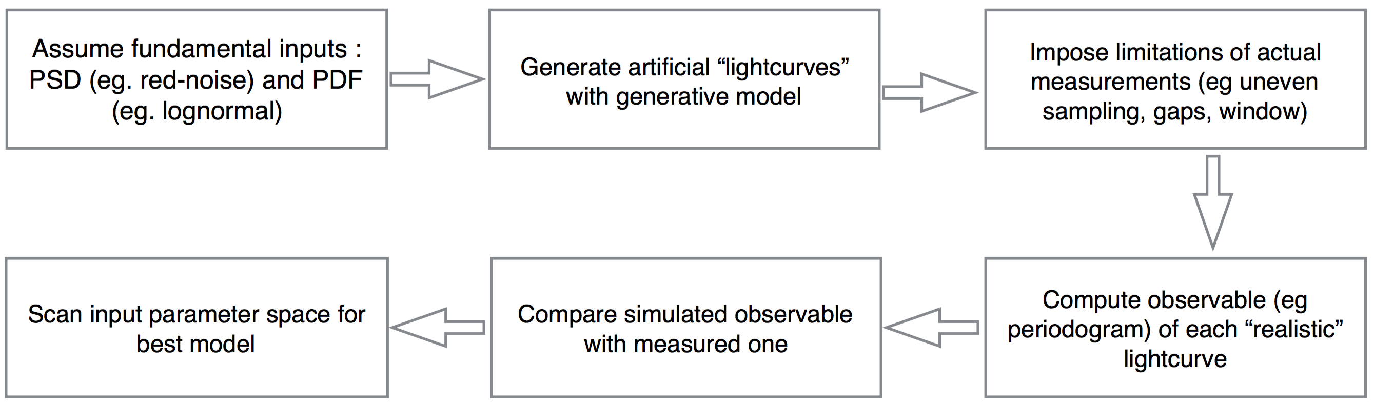
Figure 2: The applied time-series method involves modifying the Timmer-Koenig method to account for lognormality and gaps (or Emmanoulopoulos method) to generate lightcurves of a given PSD and PDF. The observed cadence, i.e., gaps, sampling and duration of the window are imposed on the simulated lightcurves. The PSD and PDF parameters that best describe the observations are evaluated by a likelihood analysis.

4 Methodological tests of PSD estimates

(a) Pink noise or $\Gamma=1.0$

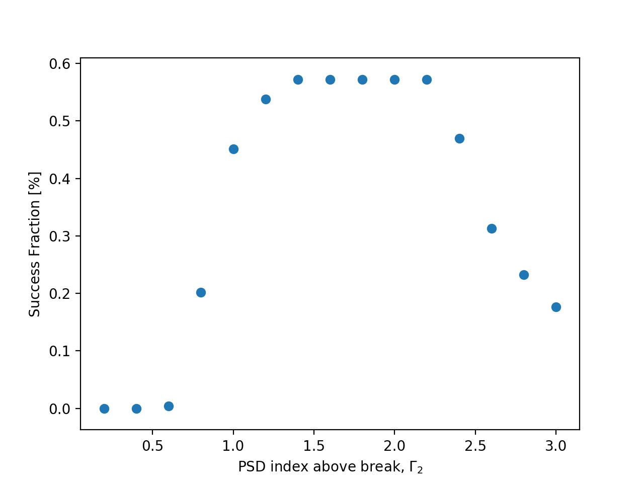
(b) Red noise or $\Gamma=2.0$

Figure 3: The figure shows comparison between the reconstruction with a broken power-law and bending power-law model (break at $\sim 640$ years) for a true power-law observation with top: pink noise and bottom: red noise characteristics. There is not a significant difference between the two models. However, it is clear that reconstructions are more challenging at greater values of index.

(a) $t_{\rm b}=6.4\times 10^{1},1.3\times 10^{2}$, and $3.2\times 10^{2}$

(b) $t_{\rm b}=6.4\times 10^{2},1.3\times 10^{3}$, and $3.2\times 10^{3}$

Figure 4: The effect of the break position on reconstructing the PSD index of simulated lightcurve matching the Fermi-LAT cadence for Mrk 421 with a power-law with index $\Gamma=1.0$. Testing with break values of $6.4\times 10^{1},1.3\times 10^{2},3.2\times 10^{2},6.4\times 10^{2},1.3\times 10^{3}$, and $3.2\times 10^{3}$, years respectively, we find the optimal value corresponding to the best reconstruction to be at $6.4\times 10^{2}$ years.

Estimates of PSD indices can get pretty involved even when the true PSD is a simple, single power-law noise. The following are some astrophysical and methodological issues that come up:

1. The flux (probability) distribution function (PDF) and PSD estimates are in general interconnected (e.g., Vaughan et al., 2003; Romoli et al., 2018; Morris et al., 2019). Indices steeper than one lead to deviations from strict stationarity and thereby Gaussianity of simulations.

2. A transition (break or smooth bend) from coloured noise to white noise can prevent the divergence of total power and remedy this problem. However, the existence of genuine astrophysical breaks will lead to poorer estimates when considering pure power-law generative models.

3. Furthermore, red-noise leakage makes the power at different frequencies dependent; this reduces the scatter at high frequencies. This can affect the estimates depending upon the break or bend frequency

The connection between variable flux PDF and PSD estimates is an important one as shown in Morris et al. (2019). For noise properties steeper than pink noise, there is a loss of strict stationarity. This results in the full PDF not being constant. In other words, higher moments including the variance are not conserved and therefore, the PSD estimates are compromised. Introducing a break or a smooth bend to flatten out the spectrum at low frequencies or longer timescales helps to ameliorate this effect. It must be noted that, a priori, such a break need not necessarily be a physical break; instead, it is introduced beyond observed timescales in order to prevent the total power at low frequencies and preserve the PDF. However, as we will see in the following, the break that allows one to reconstruct the indices correctly, turns out to be compatible with the physically motivated value. Introducing a break at a Fourier frequency outside of the observed range works rather well at preserving the normal behaviour of TK lightcurves. This can be seen by evaluating the Gaussianity of simulated lightcurves as e.g. done for Mrk 421 in Chakraborty (2020). These results are in principle subject to the assumptions that the simulations themselves are consistent with a normal distribution as assumed in the TK approach. Generalizations to lognormal ensembles, however, can be done by exponentiating the fluxes with the appropriate transformed mean and variance, which implies that the log of fluxes follow a normal distribution (Uttley et al., 2005). This presumes that the simulated TK95 lightcurve follow the Gaussian distribution specified at the input. Performing tests of Gaussianity on the simulations tests this. Note the vast difference between the fraction of simulations rejected for the PSD index 2.0 relative to index 1.0 as shown in Morris et al. (2019). This shows clearly that the pure PL ensemble does not preserve Gaussianity. This would also mean that the lognormal simulations which are obtained by the exponential transform from Gaussian simulations, do not preserve the lognormal distribution.

5 PSD estimation

We use simulated lightcurves obtained following the description in section 3 to explore the quality of PSD reconstruction.

We simulate lightcurves for a range of PSD power-law indices from 0.2 to 3.0 for a normal PDF with mean and variance to match those of the Fermi-LAT  observations of Mrk 421 as an example. These artificial lightcurves need to match the observed mean and variance to be "realistic". We choose a frequency range from $f_{\rm min}$ (or $T_{\rm max}$, e.g., related to the observation time, $T_{\rm obs}$) and $f_{\rm max}$ (or $T_{\rm min}$, i.e., related to the bin size, $T_{\rm bin}$). When the simulations have a finer binning, we average simulated fluxes around the observed time $t_{\rm bin}$. However, in most cases we simulate the exact cadence of the observations. The gaps would naturally be retained as gaps in order to fold in their effects. We then estimate the "best" PSD as prescribed in (Chatterjee et al., 2008). We compute the deviation in chi-square from within the simulations, $\chi^{2}_{\rm sim}$, relative to its mean. We also compute the chi-square of the simulations relative to observations, $\chi^{2}_{\rm obs}$. Comparing the two, we can determine the fraction of simulations for which the chi-square relative to observations is less than that with respect to simulations themselves. This is the success fraction, showing the fraction of cases, wherein the observations are compatible with simulations to within the dispersion of the simulations.

5.1 Break position - Reconstructing index for simulated lightcurves with known values

To probe if there is a universal parametrization of the position of the break that may be applicable to lightcurves in general, we use simulations to reconstruct the PSD index of a mock observation. Note that when performing such tests with simulations, the mock observation or lighcurve may in principle be generated by a PL, BPL or BrPL model following eqs. (1)-(3). And if there is a physical break outside of the observational bandwidth of frequencies [$f_{\rm min},f_{\rm max}$], then the observation is in effect, one realisation of such a process that can be parametrised by a BPL or BrPL model. Therefore, in this scenario to be fully self-consistent, one should use BPL for both, the mock observation and the ensemble. Obviously, as we do not know the break value ($f_{\rm b}$) apriori, in general we would need to explore the reconstruction of both, the break value and the index $\Gamma$. However, this will require a full 2D exploration or more generally a multidimensional exploration of all the PSD and PDF parameters. This is beyond the scope of this paper and will be reserved for a future work. Here for simplicity, we run tests to see how well the index of a PL mock observation is reconstructed by BPL and BrPL simulations. This is illustrated by the example in figure 3. Clearly, reconstructions are subject to noise for stochastic processes generating lightcurves. Upon investigation, we find that the BrPL model does not necessarily have an advantage compared to the BPL model. The former does not guarantee a better reconstruction. On the other hand, the smoother BPL is a more physical parametrization. Therefore we will focus in the following on the BPL model. From hereon we also do not distinguish between break and bend and use them interchangeably.

The BPL model of the form in eq. ( 2) is used to generate the ensemble with a range of indices $\Gamma$. We then compare each member with the mock observed lightcurve. We compute the reduced chi-square, $\bigg{(}\chi^{2}/\nu\bigg{)}_{\rm i}$ from the difference of simulated and observed periodogram for each ensemble member. We then compare with the mean reduced chi-square, $\bigg{(}\chi^{2}/\nu\bigg{)}_{\rm mean}$ that measures the dispersion within the ensemble. The fraction of simulations, $m$, for which the deviation of the mock observation from the ensemble is less than the ensemble dispersion, $\bigg{(}\chi^{2}/\nu\bigg{)}_{\rm i}<\bigg{(}\chi^{2}/\nu\bigg{)}_{\rm mean}$ quantifies the probability of the model PSD (parameter) fitting the observation. The simulated index with the highest fraction $m$ is the best fit index value. The absolute value of $m$ is indicative of how well a model with a certain level of complexity or number of parameters describes the features of the observed lightcurve relative to the natural statistical dispersion of the simulations with that model. We then repeat this for different break frequencies, $f_{\rm break}$.

For our artificial lightcurves, the considered estimation will reconstruct the true power-law PSD index the best, when the position of the break, $f_{\rm b}$ is sufficiently lower than the minimum Fourier frequency of the observation window, $f_{\rm min}=1/t_{\rm max}=1/t_{\rm obs}$. This is because if $f_{\rm b}$ is too close to $f_{\rm min}$, then the transition to white noise will reduce the power in the observed band, [$f_{\rm min},f_{\rm max}$] and produce a deviation from the true power-law. The obvious caveat is if the true PSD itself would have a physical break, such as related to the viscous timescale in the disk (cf. Sec. 2) or associated with particle cooling (Finke and Becker, 2014), and be close to being detected.

For convenience, we employ a parameterization for the break position of the form,

$$\left(\frac{f_{\rm break}}{1~{}{\mathrm{day}}^{-1}}\right)=\frac{1}{\alpha}\frac{t_{\rm bin}}{t_{\rm obs}}\,$$ (5)

where $\alpha$ is a "lengthening" multiplicative factor. The ratio of the bin size $t_{\rm bin}$ and the length of the observation window, $t_{\rm obs}$, represents the dynamic range and is a natural scale to consider. Hence, $\alpha$ essentially parameterizes, how many times this dimensionless scale the frequency break is placed at. For the considered Fermi-LAT observations of Mrk 421 with a duration of about 6.5 years and a bin size of 10 days (Sinha et al., 2016), $t_{\rm bin}/t_{\rm obs}\simeq 4.2\times 10^{-3}$. Therefore, a factor of e.g., $\alpha=1000$ would correspond to a break frequency, $f_{\rm b}\simeq 4.2\times 10^{-6}{\rm day^{-1}}$, corresponding to a timescale of $t_{b}\simeq 640$ years.

Our simulated lightcurves each have a length of 2340 days, corresponding to the length of the Fermi-LAT observations of Mrk 421, with the same bin size of 10 days.

The factor, $\alpha$ is set to values 100, 200, 300, 500, 1000 and 3000 which corresponds to break or bending timescales of $t_{b}=6.4\times 10^{1}$, $1.3\times 10^{2}$, $1.9\times 10^{2}$, $3.2\times 10^{2}$, $6.4\times 10^{2}$ and $1.9\times 10^{3}$ years, respectively. We then perform estimation of the index of these "mock observed lightcurves" with the methodology described above. Naturally, using artificial lightcurves, we expect the estimates to match the chosen index value, e.g., $1.0$, used to generate the lightcurves in the first place. As shown in Figure 4, the value of $\alpha=1000$ corresponding to $t_{b}=6.4\times 10^{2}$ yrs gives the sharpest reconstruction of the correct index. The predictions work better with index $\lesssim 1$, though even for indices $>1$, the predictions seem to be much better than when affected by non-stationarity. We also ran a few trial runs with the DE13 method. From these, it was unclear that there is any advantage vis-a-vis precision for the available data especially for indices greater than 1.0, and given the computational cost of the DE13, the bending power-law seems advantageous especially for simpler PSD models. The effects of a more complex input model of PSD and PDF needs a dedicated paper and is left for the future. Thus, given the advantage in terms of accuracy and precision of DE13 is not clear for the longest timescales and the computational cost is high, the use of a BPL model that is faster and easier to interpret is advantageous.

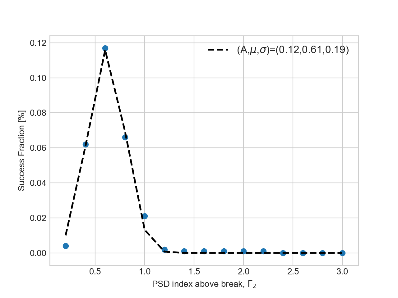
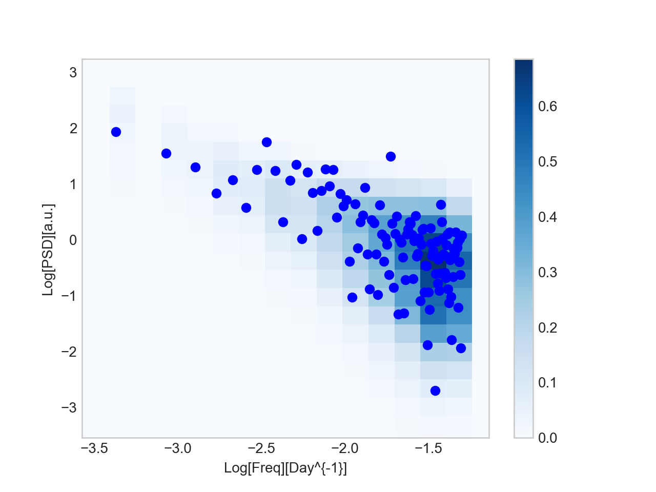
Figure 5: The PSD index of the Fermi-LAT lightcurve determined with a break factor of 1000 or $t_{\rm b}\approx 640$ years. Top: From the chi-square test, the maximum number of simulations prefer an index of value $\Gamma\approx 0.6$. Note that this does not account for a bias which from our tests is $\approx 0.2$. Bottom: The probability map quantifying number of simulations that have a certain power density in a given frequency bin is shown. The blue circles are the periodogram directly obtained from the observed Fermi-LAT lightcurves. The color bar represents the fraction of simulations in any given bin having been normalised to the total number of simulations.

5.2 PSD of LAT and BAT lightcurve

Having tested on mock longterm lightcurves of timescales of a few years, we now evaluate the PSD of Fermi-LAT and Swift-BAT lightcurves of Mrk 421. The length of both of these lightcurves is comparable at $\sim 2000$ days or $\sim 7$ years. Furthermore, the binning is at around 10 days. We therefore, pick the "optimal" simulation break factor determined from our tests at $t_{\rm b}\approx 640$ years or break factor, $\alpha=1000$. The analysis in Chakraborty (2020) indicates that the preferred distribution for the Fermi-LAT lightcurves is lognormal and even for Swift-BAT, the lognormal PDF matches the high flux tail. Hence, for the simulated ensemble we use the lognormal function as input PDF. With these, we perform the reduced chi-square test (Chatterjee et al., 2008), scanning index values in the We also provide the probability map - the two-dimensional histogram of power spectral density of the simulated ensemble with these indices, stacked upon each other and the periodogram of the lightcurves. The top panels of figures (5) and  (6) show the success fraction as a function of index and the bottom panels show the PSD map for the Fermi-LAT and Swift-BAT lightcurves, respectively. In both cases, the maps show that the scatter of the PSD for observed cadence (10 days) is at the level of the average dispersion of the simulations. This shows that the good quality of monitoring with Fermi-LAT and Swift-BAT allows for a relatively precise estimate of the long-term stochastic properties. The peak of $m$ for the Fermi-LAT case is well defined but has a value of only $\sim 12\%$ similar to Fermi-LAT and OVRO results in Goyal (2020). This suggests that of the BPL or "PL with smooth break/bend models", the "best" choice is index $\sim 0.6$. This is a sense a reduced BPL model as we fix the lower index (below break) to zero, and while determining best higher index (above break) we fix the break frequency to the optimal one obtained from simulations for the cadence. The low $m$ values indicate, these simple models are not sufficient to explain the observations and we need to explore more complex models. The natural next step would be to jointly explore the space of break and the index above it, as we have already indicated in section (5.1). This reduced BPL model seems to work much better for Swift-BAT lightcurves. This is consistent with the probability or PSD maps. The BAT maps and blue data points in figure 6 appear to have more of a mean PL type behaviour about which there is scatter and the best $\Gamma$ describing this has a central value of 0.8. Relatively, the LAT maps have a slight hint of curvature. However, a definitive conclusion on this would depend upon full multi-dimensional parameter estimation.

As mentioned, we find that for the Fermi-LAT lightcurve, the index obtained from the reduced chi-square test is $\Gamma\approx 0.6$ whereas for the Swift-BAT lightcurve we obtain $\Gamma\approx 0.8$. The uncertainty quantification derives from parameter estimation by varying the relevant model parameters (in this case, the PSD index) in an appropriately wide range and freezing other parameters (as e.g. done in Goyal, 2020). Estimates of the statistical uncertainty are made here by fitting a Gaussian to the success fraction, giving $0.2$ for both lightcurves. Neither of these values account for a systematic bias as inferred from our methodological tests using mock observations with known index, whose value is $\sim 0.2$. This value denotes the difference between the reconstructed index value where the success fraction peaks and the true value of the index for simulated or mock observations. Accordingly, the LAT and BAT lightcurves are characterized by PSDs with an index above the break, $\Gamma=0.6\pm 0.2^{stat}+0.2^{sys}$ and $\Gamma=0.8\pm 0.2^{stat}+0.2^{sys}$, respectively.

Our findings for Mrk 421 can be compared with related results in the literature. Goyal (2020), for example, report PSD indices of $1.1\pm 0.4$, $1.3\pm 0.7$ and $1.1\pm 1.6$ for Fermi-LAT , Swift-XRT (0.3-10 keV) and RXTE-PCA (3-20 keV) lightcurves, respectively. The Fermi-LAT result is compatible, within errors, with pink noise, while their X-ray estimate is not well-constrained. Chatterjee et al. (2018), on the other hand, find that in the X-rays the extended, short- to long-term PSD is compatible with a bending PL model (breaking from $\Gamma\simeq 1.2\pm 0.5$ to $\Gamma\simeq 2.5\pm 0.5$ at a high-frequency break corresponding to $\sim 10$ d). While this indicates that the extended PSD can show further bends or breaks, the longterm PSD estimate ($1.2\pm 0.5$) is again compatible with pink noise. This compares well with our findings reported here. For the transition between different regimes, especially at shorter timescales, an extended examination of the PSD and break at timescales of days would be needed, which is not the focus of this work. Note that the break frequency we employ corresponds to a break time of about $T_{b}\simeq 640$ yr. This is close to the viscous timescale at the disk truncation radius, considering a characteristic black hole mass in Mrk 421 of $M_{\rm BH}\sim 2\times 10^{8}M_{\odot}$ (e.g., Barth et al., 2003).

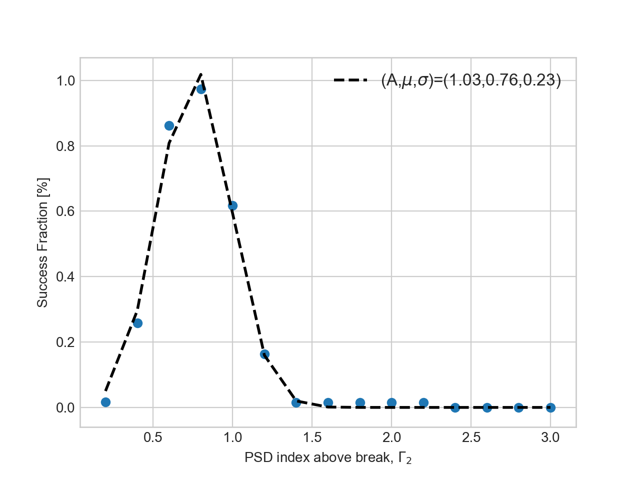
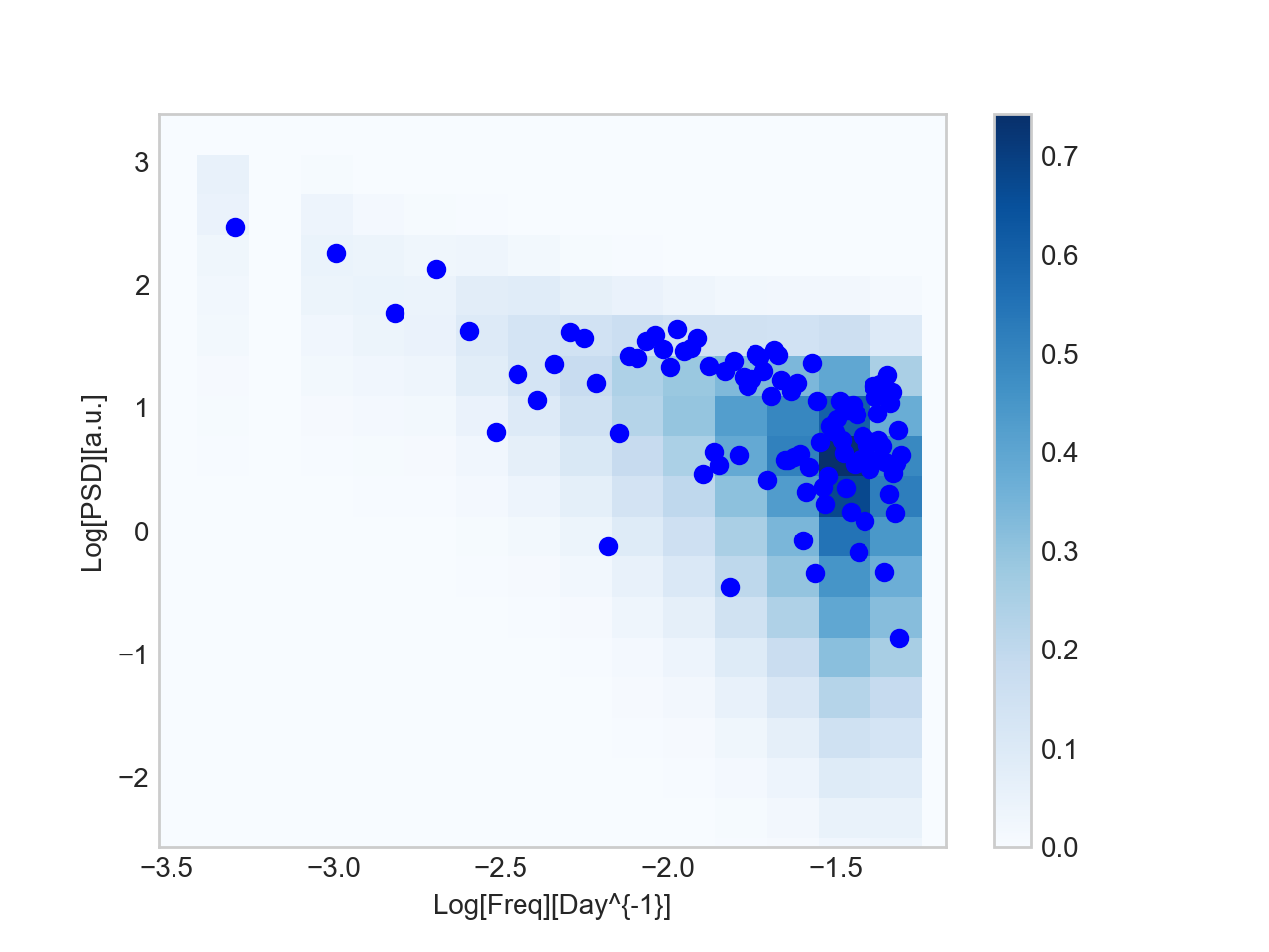
Figure 6: Figure shows the PSD index of the Swift-BAT lightcurve determined with a break factor of 1000 or $t_{b}\approx 640$ years assuming a Lognormal PDF. Top: From the chi-square test, the maximum number of simulations prefer an index of value $\Gamma\approx 0.8$. Note that this does not account for a bias which from the tests earlier is $\approx 0.2$. Bottom: The simulated probability map for Swift-BAT lightcurves as well as the periodogram of the observation as in fig. (5).

6 Discussion and Conclusions

Quantifying the power spectral density is the key to understanding the stochastic behaviour of a variable source such as an AGN or XRB. Features such as breaks can be indicators of physical timescales and therefore processes and transitions between them (Finke and Becker, 2014; Rieger, 2019). Knowing the PSD is also important in order to test the true significance of a genuine quasi-periodic oscillation against false alarms from noisy variability (Ait Benkhali et al., 2020; Vaughan et al., 2016). Several methods have been developed to quantifying the PSD (Timmer and Koenig, 1995; Emmanoulopoulos et al., 2013). Central to estimating the PSD is the implicit assumption, in most cases, of weak non-stationarity. It has been shown that this is not guaranteed and is crucially compromised at larger values of PSD index (Vaughan et al., 2003; Morris et al., 2019). This is due to divergence of the variance (second moment of the underlying distribution) or integral power of the variability in the limit of infinite bandwidth as the index exceeds values $1-1.5$. In practice, for large enough bandwidths such as in the case of long term monitoring discussed here ($[t_{\rm min},t_{\rm max}]=$ [days,years]), this effect is already pronounced as shown in (Morris et al., 2019). The "redder" the random noise in variability, the lower is the fraction of realisations of the process which preserve same probability density function (PDF). Therefore, the statistical estimation of the PSD index and other stochastic properties dependent on it, is compromised for a range of values $(\gtrsim 1)$. Here in this work, we seek to find a way to assuage this problem. A bending power-law (BPL) PSD model inspired by OU type processes is used. The smooth transition to white noise from coloured noise prevents this divergence of power and is also a realistic model of high energy variability over a range of timescales from weeks to many years. In principle, we expect a characteristic low-frequency bend or break corresponding to the viscosity timescale at the disk truncation radius, $t_{\rm visc}$, which in turn depends upon the mass of the central supermassive black hole. Typical values range from hundreds to thousands of years. We find that this timescale is a reasonable guess for a methodological break timescale, $t_{\rm b}$, which prevents the divergence and provides a good reconstruction of index values for variability over weeks to years. Additionally, by virtue of being a simple modification of the PSD model as opposed to a fully general model of the variability (with multiple free parameters for the PSD and PDF), it is computationally very fast. This method is applied to X-ray (Swift-BAT) and gamma-ray (Fermi-LAT ) long term lightcurves of the source Mrk 421 spanning nearly 7 years. The reconstructed PSD values for both lightcurves are in principle compatible with pink (flicker) noise, given the uncertainty and bias in the estimate, though there seems to be a tendency for a slightly flatter value at gamma-ray energies. These findings are broadly compatible with previous results (Chatterjee et al., 2018; Goyal, 2020). Our evaluation with the BPL model also provides realistic estimates of statistical and systematic uncertainty (each $\lesssim 25\%$) with the success fraction from reduced chi-square (Chatterjee et al., 2008). This makes the estimate a rather robust one. We note that for a full reconstruction of variability parameters, we cannot avoid a multi-dimensional parameter reconstruction. This will be the subject of a future investigation. In general, quantifying the variability properties of a source is inherently, multi-observable problem. The PSD quantifies the underlying stochasticity and the PDF encodes the form of the driving mechanism. As found in Morris et al. (2019), these estimates are interlinked. However, making certain reasonable assumptions about one, one can investigate the other. In this way, any limitations of the estimate are made explicit and reliability is proportional to the quality of the data. For getting such an estimate of the index for a simple model (e.g., power-law regime) of stochasticity in the long-term variations, the use of a BPL model with a bend frequency comparable to viscous timescale at the disk truncation radius, $f_{b}\sim 1/t_{\rm b}$, is a physically motivated, efficient and accurate solution.

7 Data Availability Statement

The data underlying this article were provided by Atreyee Sinha by permission. Data will be shared on request to the corresponding author with her permission.

References

- Ackermann et al. [2015] M. Ackermann, M. Ajello, A. Albert, W. B. Atwood, L. Baldini, J. Ballet, G. Barbiellini, D. Bastieri, J. Becerra Gonzalez, R. Bellazzini, E. Bissaldi, R. D. Blandford, E. D. Bloom, R. Bonino, E. Bottacini, J. Bregeon, P. Bruel, R. Buehler, S. Buson, G. A. Caliandro, R. A. Cameron, R. Caputo, M. Caragiulo, P. A. Caraveo, E. Cavazzuti, C. Cecchi, A. Chekhtman, J. Chiang, G. Chiaro, S. Ciprini, J. Cohen-Tanugi, J. Conrad, S. Cutini, F. D’Ammand o, A. de Angelis, F. de Palma, R. Desiante, L. Di Venere, A. Domínguez, P. S. Drell, C. Favuzzi, S. J. Fegan, E. C. Ferrara, W. B. Focke, L. Fuhrmann, Y. Fukazawa, P. Fusco, F. Gargano, D. Gasparrini, N. Giglietto, P. Giommi, F. Giordano, M. Giroletti, G. Godfrey, D. Green, I. A. Grenier, J. E. Grove, S. Guiriec, A. K. Harding, E. Hays, J. W. Hewitt, A. B. Hill, D. Horan, T. Jogler, G. Jóhannesson, A. S. Johnson, T. Kamae, M. Kuss, S. Larsson, L. Latronico, J. Li, L. Li, F. Longo, F. Loparco, B. Lott, M. N. Lovellette, P. Lubrano, J. Magill, S. Maldera, A. Manfreda, W. Max-Moerbeck, M. Mayer, M. N. Mazziotta, J. E. McEnery, P. F. Michelson, T. Mizuno, M. E. Monzani, A. Morselli, I. V. Moskalenko, S. Murgia, E. Nuss, M. Ohno, T. Ohsugi, R. Ojha, N. Omodei, E. Orlando, J. F. Ormes, D. Paneque, T. J. Pearson, J. S. Perkins, M. Perri, M. Pesce-Rollins, V. Petrosian, F. Piron, G. Pivato, T. A. Porter, S. Rainò, R. Rando, M. Razzano, A. Readhead, A. Reimer, O. Reimer, A. Schulz, C. Sgrò, E. J. Siskind, F. Spada, G. Spandre, P. Spinelli, D. J. Suson, H. Takahashi, J. B. Thayer, D. J. Thompson, L. Tibaldo, D. F. Torres, G. Tosti, E. Troja, Y. Uchiyama, G. Vianello, K. S. Wood, M. Wood, S. Zimmer, A. Berdyugin, R. H. D. Corbet, T. Hovatta, E. Lindfors, K. Nilsson, R. Reinthal, A. Sillanpää, A. Stamerra, L. O. Takalo, and M. J. Valtonen. Multiwavelength Evidence for Quasi-periodic Modulation in the Gamma-Ray Blazar PG 1553+113. ApJL, 813(2):L41, November 2015. doi: 10.1088/2041-8205/813/2/L41.
- Vaughan et al. [2016] S. Vaughan, P. Uttley, A. G. Markowitz, D. Huppenkothen, M. J. Middleton, W. N. Alston, J. D. Scargle, and W. M. Farr. False periodicities in quasar time-domain surveys. MNRAS, 461(3):3145–3152, September 2016. doi: 10.1093/mnras/stw1412.
- Covino et al. [2019] S. Covino, A. Sandrinelli, and A. Treves. Gamma-ray quasi-periodicities of blazars. A cautious approach. MNRAS, 482(1):1270–1274, January 2019. doi: 10.1093/mnras/sty2720.
- Ait Benkhali et al. [2020] F. Ait Benkhali, W. Hofmann, F. M. Rieger, and N. Chakraborty. Evaluating quasi-periodic variations in the -ray light curves of Fermi-LAT blazars. AAP, 634:A120, February 2020. doi: 10.1051/0004-6361/201935117.
- Timmer and Koenig [1995] J. Timmer and M. Koenig. On generating power law noise. AAP, 300:707, August 1995.
- Vaughan [2013] Simon Vaughan. Random time series in Astronomy. arXiv e-prints, art. arXiv:1309.6435, Sep 2013.
- Rieger [2019] Frank Rieger. Gamma-Ray Astrophysics in the Time Domain. Galaxies, 7(1):28, Jan 2019. doi: 10.3390/galaxies7010028.
- Uttley et al. [2002] P. Uttley, I. M. McHardy, and I. E. Papadakis. Measuring the broad-band power spectra of active galactic nuclei with RXTE. MNRAS, 332:231–250, May 2002. doi: 10.1046/j.1365-8711.2002.05298.x.
- Uttley et al. [2005] P. Uttley, I. M. McHardy, and S. Vaughan. Non-linear X-ray variability in X-ray binaries and active galaxies. MNRAS, 359:345–362, May 2005. doi: 10.1111/j.1365-2966.2005.08886.x.
- Vaughan et al. [2003] S. Vaughan, R. Edelson, R. S. Warwick, and P. Uttley. On characterizing the variability properties of X-ray light curves from active galaxies. MNRAS, 345:1271–1284, November 2003. doi: 10.1046/j.1365-2966.2003.07042.x.
- Morris et al. [2019] Paul J. Morris, Nachiketa Chakraborty, and Garret Cotter. Deviations from normal distributions in artificial and real time series: a false positive prescription. MNRAS, 489(2):2117–2129, Oct 2019. doi: 10.1093/mnras/stz2259.
- Abdo et al. [2010] A. A. Abdo, M. Ackermann, M. Ajello, E. Antolini, L. Baldini, J. Ballet, G. Barbiellini, D. Bastieri, K. Bechtol, R. Bellazzini, B. Berenji, R. D. Blandford, E. D. Bloom, E. Bonamente, A. W. Borgland, A. Bouvier, J. Bregeon, A. Brez, M. Brigida, P. Bruel, R. Buehler, T. H. Burnett, S. Buson, G. A. Caliand ro, R. A. Cameron, P. A. Caraveo, S. Carrigan, J. M. Casandjian, E. Cavazzuti, C. Cecchi, Ö. Çelik, A. Chekhtman, C. C. Cheung, J. Chiang, S. Ciprini, R. Claus, J. Cohen-Tanugi, L. R. Cominsky, J. Conrad, L. Costamante, S. Cutini, C. D. Dermer, A. de Angelis, F. de Palma, E. do Couto e. Silva, P. S. Drell, R. Dubois, D. Dumora, C. Farnier, C. Favuzzi, S. J. Fegan, W. B. Focke, P. Fortin, M. Frailis, Y. Fukazawa, S. Funk, P. Fusco, F. Gargano, D. Gasparrini, N. Gehrels, S. Germani, B. Giebels, N. Giglietto, P. Giommi, F. Giordano, T. Glanzman, G. Godfrey, I. A. Grenier, M. H. Grondin, J. E. Grove, S. Guiriec, D. Hadasch, M. Hayashida, E. Hays, S. E. Healey, D. Horan, R. E. Hughes, R. Itoh, G. Jóhannesson, A. S. Johnson, W. N. Johnson, T. Kamae, H. Katagiri, J. Kataoka, N. Kawai, J. Knödlseder, M. Kuss, J. Lande, S. Larsson, L. Latronico, M. Lemoine-Goumard, F. Longo, F. Loparco, B. Lott, M. N. Lovellette, P. Lubrano, G. M. Madejski, A. Makeev, E. Massaro, M. N. Mazziotta, J. E. McEnery, P. F. Michelson, W. Mitthumsiri, T. Mizuno, A. A. Moiseev, C. Monte, M. E. Monzani, A. Morselli, I. V. Moskalenko, M. Mueller, S. Murgia, P. L. Nolan, J. P. Norris, E. Nuss, M. Ohno, T. Ohsugi, N. Omodei, E. Orlando, J. F. Ormes, M. Ozaki, J. H. Panetta, D. Parent, V. Pelassa, M. Pepe, M. Pesce-Rollins, F. Piron, T. A. Porter, S. Rainò, R. Rando, M. Razzano, A. Reimer, O. Reimer, S. Ritz, A. Y. Rodriguez, R. W. Romani, M. Roth, F. Ryde, H. F. W. Sadrozinski, A. Sand er, J. D. Scargle, C. Sgrò, M. S. Shaw, P. D. Smith, G. Spandre, P. Spinelli, J. L. Starck, M. S. Strickman, D. J. Suson, H. Takahashi, T. Takahashi, T. Tanaka, J. B. Thayer, J. G. Thayer, D. J. Thompson, L. Tibaldo, D. F. Torres, G. Tosti, A. Tramacere, Y. Uchiyama, T. L. Usher, V. Vasileiou, N. Vilchez, V. Vitale, A. P. Waite, E. Wallace, P. Wang, B. L. Winer, K. S. Wood, Z. Yang, T. Ylinen, and M. Ziegler. Gamma-ray Light Curves and Variability of Bright Fermi-detected Blazars. ApJ, 722(1):520–542, October 2010. doi: 10.1088/0004-637X/722/1/520.
- Ackermann et al. [2011] M. Ackermann, M. Ajello, A. Allafort, E. Antolini, W. B. Atwood, M. Axelsson, L. Baldini, J. Ballet, G. Barbiellini, D. Bastieri, K. Bechtol, R. Bellazzini, B. Berenji, R. D. Blandford, E. D. Bloom, E. Bonamente, A. W. Borgland, E. Bottacini, A. Bouvier, J. Bregeon, M. Brigida, P. Bruel, R. Buehler, T. H. Burnett, S. Buson, G. A. Caliandro, R. A. Cameron, P. A. Caraveo, J. M. Casand jian, E. Cavazzuti, C. Cecchi, E. Charles, C. C. Cheung, J. Chiang, S. Ciprini, R. Claus, J. Cohen-Tanugi, J. Conrad, L. Costamante, S. Cutini, A. de Angelis, F. de Palma, C. D. Dermer, S. W. Digel, E. do Couto e. Silva, P. S. Drell, R. Dubois, L. Escande, C. Favuzzi, S. J. Fegan, E. C. Ferrara, J. Finke, W. B. Focke, P. Fortin, M. Frailis, Y. Fukazawa, S. Funk, P. Fusco, F. Gargano, D. Gasparrini, N. Gehrels, S. Germani, B. Giebels, N. Giglietto, P. Giommi, F. Giordano, M. Giroletti, T. Glanzman, G. Godfrey, I. A. Grenier, J. E. Grove, S. Guiriec, M. Gustafsson, D. Hadasch, M. Hayashida, E. Hays, S. E. Healey, D. Horan, X. Hou, R. E. Hughes, G. Iafrate, G. Jóhannesson, A. S. Johnson, W. N. Johnson, T. Kamae, H. Katagiri, J. Kataoka, J. Knödlseder, M. Kuss, J. Lande, S. Larsson, L. Latronico, F. Longo, F. Loparco, B. Lott, M. N. Lovellette, P. Lubrano, G. M. Madejski, M. N. Mazziotta, W. McConville, J. E. McEnery, P. F. Michelson, W. Mitthumsiri, T. Mizuno, A. A. Moiseev, C. Monte, M. E. Monzani, E. Moretti, A. Morselli, I. V. Moskalenko, S. Murgia, T. Nakamori, M. Naumann-Godo, P. L. Nolan, J. P. Norris, E. Nuss, M. Ohno, T. Ohsugi, A. Okumura, N. Omodei, M. Orienti, E. Orlando, J. F. Ormes, M. Ozaki, D. Paneque, D. Parent, M. Pesce-Rollins, M. Pierbattista, S. Piranomonte, F. Piron, G. Pivato, T. A. Porter, S. Rainò, R. Rando, M. Razzano, S. Razzaque, A. Reimer, O. Reimer, S. Ritz, L. S. Rochester, R. W. Romani, M. Roth, D. A. Sanchez, C. Sbarra, J. D. Scargle, T. L. Schalk, C. Sgrò, M. S. Shaw, E. J. Siskind, G. Spandre, P. Spinelli, A. W. Strong, D. J. Suson, H. Tajima, H. Takahashi, T. Takahashi, T. Tanaka, J. G. Thayer, J. B. Thayer, D. J. Thompson, L. Tibaldo, M. Tinivella, D. F. Torres, G. Tosti, E. Troja, Y. Uchiyama, J. Vandenbroucke, V. Vasileiou, G. Vianello, V. Vitale, A. P. Waite, E. Wallace, P. Wang, B. L. Winer, D. L. Wood, K. S. Wood, and S. Zimmer. The Second Catalog of Active Galactic Nuclei Detected by the Fermi Large Area Telescope. ApJ, 743(2):171, December 2011. doi: 10.1088/0004-637X/743/2/171.
- Sobolewska et al. [2014] M. A. Sobolewska, A. Siemiginowska, B. C. Kelly, and K. Nalewajko. Stochastic Modeling of the Fermi/LAT -Ray Blazar Variability. ApJ, 786:143, May 2014. doi: 10.1088/0004-637X/786/2/143.
- Max-Moerbeck et al. [2014] W. Max-Moerbeck, T. Hovatta, J. L. Richards, O. G. King, T. J. Pearson, A. C. S. Readhead, R. Reeves, M. C. Shepherd, M. A. Stevenson, E. Angelakis, L. Fuhrmann, K. J. B. Grainge, V. Pavlidou, R. W. Romani, and J. A. Zensus. Time correlation between the radio and gamma-ray activity in blazars and the production site of the gamma-ray emission. MNRAS, 445(1):428–436, November 2014. doi: 10.1093/mnras/stu1749.
- H.E.S.S. Collaboration et al. [2017] H.E.S.S. Collaboration, H. Abdalla, A. Abramowski, F. Aharonian, F. Ait Benkhali, A. G. Akhperjanian, T. Andersson, E. O. Angüner, M. Arrieta, P. Aubert, M. Backes, A. Balzer, M. Barnard, Y. Becherini, J. Becker Tjus, D. Berge, S. Bernhard, K. Bernlöhr, R. Blackwell, M. Böttcher, C. Boisson, J. Bolmont, P. Bordas, J. Bregeon, F. Brun, P. Brun, M. Bryan, T. Bulik, M. Capasso, J. Carr, S. Casanova, M. Cerruti, N. Chakraborty, R. Chalme-Calvet, R. C. G. Chaves, A. Chen, J. Chevalier, M. Chrétien, S. Colafrancesco, G. Cologna, B. Condon, J. Conrad, Y. Cui, I. D. Davids, J. Decock, B. Degrange, C. Deil, J. Devin, P. deWilt, L. Dirson, A. Djannati-Ataï, W. Domainko, A. Donath, L. O. ’C. Drury, G. Dubus, K. Dutson, J. Dyks, T. Edwards, K. Egberts, P. Eger, J. P. Ernenwein, S. Eschbach, C. Farnier, S. Fegan, M. V. Fernand es, A. Fiasson, G. Fontaine, A. Förster, S. Funk, M. Füßling, S. Gabici, M. Gajdus, Y. A. Gallant, T. Garrigoux, G. Giavitto, B. Giebels, J. F. Glicenstein, D. Gottschall, A. Goyal, M. H. Grondin, D. Hadasch, J. Hahn, M. Haupt, J. Hawkes, G. Heinzelmann, G. Henri, G. Hermann, O. Hervet, J. A. Hinton, W. Hofmann, C. Hoischen, M. Holler, D. Horns, A. Ivascenko, A. Jacholkowska, M. Jamrozy, M. Janiak, D. Jankowsky, F. Jankowsky, M. Jingo, T. Jogler, L. Jouvin, I. Jung-Richardt, M. A. Kastendieck, K. Katarzyński, U. Katz, D. Kerszberg, B. Khélifi, M. Kieffer, J. King, S. Klepser, D. Klochkov, W. Kluźniak, D. Kolitzus, Nu. Komin, K. Kosack, S. Krakau, M. Kraus, F. Krayzel, P. P. Krüger, H. Laffon, G. Lamanna, J. Lau, J. P. Lees, J. Lefaucheur, V. Lefranc, A. Lemière, M. Lemoine-Goumard, J. P. Lenain, E. Leser, T. Lohse, M. Lorentz, R. Liu, R. López-Coto, I. Lypova, V. Marandon, A. Marcowith, C. Mariaud, R. Marx, G. Maurin, N. Maxted, M. Mayer, P. J. Meintjes, M. Meyer, A. M. W. Mitchell, R. Moderski, M. Mohamed, L. Mohrmann, K. Morra, E. Moulin, T. Murach, M. de Naurois, F. Niederwanger, J. Niemiec, L. Oakes, P. O’Brien, H. Odaka, S. Öttl, S. Ohm, M. Ostrowski, I. Oya, M. Padovani, M. Panter, R. D. Parsons, N. W. Pekeur, G. Pelletier, C. Perennes, P. O. Petrucci, B. Peyaud, Q. Piel, S. Pita, H. Poon, D. Prokhorov, H. Prokoph, G. Pühlhofer, M. Punch, A. Quirrenbach, S. Raab, A. Reimer, O. Reimer, M. Renaud, R. de los Reyes, F. Rieger, C. Romoli, S. Rosier-Lees, G. Rowell, B. Rudak, C. B. Rulten, V. Sahakian, D. Salek, D. A. Sanchez, A. Santangelo, M. Sasaki, R. Schlickeiser, F. Schüssler, A. Schulz, U. Schwanke, S. Schwemmer, M. Settimo, A. S. Seyffert, N. Shafi, I. Shilon, R. Simoni, H. Sol, F. Spanier, G. Spengler, F. Spies, Ł. Stawarz, R. Steenkamp, C. Stegmann, F. Stinzing, K. Stycz, I. Sushch, J. P. Tavernet, T. Tavernier, A. M. Taylor, R. Terrier, L. Tibaldo, D. Tiziani, M. Tluczykont, C. Trichard, R. Tuffs, Y. Uchiyama, D. J. van der Walt, C. van Eldik, C. van Rensburg, B. van Soelen, G. Vasileiadis, J. Veh, C. Venter, A. Viana, P. Vincent, J. Vink, F. Voisin, H. J. Völk, T. Vuillaume, Z. Wadiasingh, S. J. Wagner, P. Wagner, R. M. Wagner, R. White, A. Wierzcholska, P. Willmann, A. Wörnlein, D. Wouters, R. Yang, V. Zabalza, D. Zaborov, M. Zacharias, A. A. Zdziarski, A. Zech, F. Zefi, A. Ziegler, and N. Żywucka. Characterizing the gamma-ray long-term variability of PKS 2155-304 with H.E.S.S. and Fermi-LAT. AAP, 598:A39, February 2017. doi: 10.1051/0004-6361/201629419.
- Kushwaha et al. [2017] Pankaj Kushwaha, Atreyee Sinha, Ranjeev Misra, K. P. Singh, and E. M. de Gouveia Dal Pino. Gamma-Ray Flux Distribution and Nonlinear Behavior of Four LAT Bright AGNs. ApJ, 849(2):138, November 2017. doi: 10.3847/1538-4357/aa8ef5.
- Bhatta and Dhital [2020] Gopal Bhatta and Niraj Dhital. The Nature of -Ray Variability in Blazars. ApJ, 891(2):120, March 2020. doi: 10.3847/1538-4357/ab7455.
- Goyal [2020] Arti Goyal. Blazar variability power spectra from radio up to TeV photon energies: Mrk 421 and PKS 2155-304. MNRAS, 494(3):3432–3448, April 2020. doi: 10.1093/mnras/staa997.
- Emmanoulopoulos et al. [2013] D. Emmanoulopoulos, I. M. McHardy, and I. E. Papadakis. Generating artificial light curves: revisited and updated. MNRAS, 433:907–927, August 2013. doi: 10.1093/mnras/stt764.
- Kelly et al. [2009] Brandon C. Kelly, Jill Bechtold, and Aneta Siemiginowska. Are the Variations in Quasar Optical Flux Driven by Thermal Fluctuations? ApJ, 698(1):895–910, June 2009. doi: 10.1088/0004-637X/698/1/895.
- Gillespie [1996] Daniel T. Gillespie. The mathematics of Brownian motion and Johnson noise. American Journal of Physics, 64(3):225–240, March 1996. doi: 10.1119/1.18210.
- Zhu and Xue [2016] S. F. Zhu and Y. Q. Xue. Using Leaked Power to Measure Intrinsic AGN Power Spectra of Red-noise Time Series. ApJ, 825(1):56, Jul 2016. doi: 10.3847/0004-637X/825/1/56.
- Lyubarskii [1997] Yu. E. Lyubarskii. Flicker noise in accretion discs. MNRAS, 292(3):679–685, Dec 1997. doi: 10.1093/mnras/292.3.679.
- Goodman [2003] Jeremy Goodman. Self-gravity and quasi-stellar object discs. MNRAS, 339(4):937–948, Mar 2003. doi: 10.1046/j.1365-8711.2003.06241.x.
- Markowitz et al. [2003] A. Markowitz, R. Edelson, S. Vaughan, P. Uttley, I. M. George, R. E. Griffiths, S. Kaspi, A. Lawrence, I. McHardy, K. Nandra, K. Pounds, J. Reeves, N. Schurch, and R. Warwick. X-Ray Fluctuation Power Spectral Densities of Seyfert 1 Galaxies. ApJ, 593:96–114, August 2003. doi: 10.1086/375330.
- Chatterjee et al. [2011] Ritaban Chatterjee, Alan P. Marscher, Svetlana G. Jorstad, Alex Markowitz, Elizabeth Rivers, Richard E. Rothschild, Ian M. McHardy, Margo F. Aller, Hugh D. Aller, Anne Lähteenmäki, Merja Tornikoski, Brandon Harrison, Iván Agudo, José L. Gómez, Brian W. Taylor, and Mark Gurwell. Connection Between the Accretion Disk and Jet in the Radio Galaxy 3C 111. ApJ, 734(1):43, June 2011. doi: 10.1088/0004-637X/734/1/43.
- Ishibashi and Courvoisier [2012] W. Ishibashi and T. J. L. Courvoisier. The physical origin of the X-ray power spectral density break timescale in accreting black holes. AAP, 540:L2, April 2012. doi: 10.1051/0004-6361/201218889.
- Ryan et al. [2019] J. L. Ryan, A. Siemiginowska, M. A. Sobolewska, and J. Grindlay. Characteristic Variability Timescales in the Gamma-Ray Power Spectra of Blazars. ApJ, 885(1):12, November 2019. doi: 10.3847/1538-4357/ab426a.
- Papadakis [2004] I. E. Papadakis. The scaling of the X-ray variability with black hole mass in active galactic nuclei. MNRAS, 348(1):207–213, February 2004. doi: 10.1111/j.1365-2966.2004.07351.x.
- Sinha et al. [2016] A. Sinha, A. Shukla, L. Saha, B. S. Acharya, G. C. Anupama, P. Bhattacharjee, R. J. Britto, V. R. Chitnis, T. P. Prabhu, B. B. Singh, and P. R. Vishwanath. Long-term study of Mkn 421 with the HAGAR Array of Telescopes. AAP, 591:A83, June 2016. doi: 10.1051/0004-6361/201628152.
- Finke and Becker [2014] Justin D. Finke and Peter A. Becker. Fourier Analysis of Blazar Variability. ApJ, 791(1):21, August 2014. doi: 10.1088/0004-637X/791/1/21.
- Chakraborty [2020] Nachiketa Chakraborty. Investigating Multiwavelength Lognormality with Simulations—Case of Mrk 421. Galaxies, 8(1):7, Jan 2020. doi: 10.3390/galaxies8010007.
- Connolly [2015] S D Connolly. A Python Code for the Emmanoulopoulos et al. [arXiv:1305.0304] Light Curve Simulation Algorithm. arXiv e-prints, art. arXiv:1503.06676, March 2015.
- Romoli et al. [2018] Carlo Romoli, Nachiketa Chakraborty, Daniela Dorner, Andrew Taylor, and Michael Blank. Flux Distribution of Gamma-Ray Emission in Blazars: The Example of Mrk 501. Galaxies, 6:135, December 2018. doi: 10.3390/galaxies6040135.
- Chatterjee et al. [2008] Ritaban Chatterjee, Svetlana G. Jorstad, Alan P. Marscher, Haruki Oh, Ian M. McHardy, Margo F. Aller, Hugh D. Aller, Thomas J. Balonek, H. Richard Miller, Wesley T. Ryle, Gino Tosti, Omar Kurtanidze, Maria Nikolashvili, Valeri M. Larionov, and Vladimir A. Hagen-Thorn. Correlated Multi-Wave Band Variability in the Blazar 3C 279 from 1996 to 2007. ApJ, 689(1):79–94, December 2008. doi: 10.1086/592598.
- Chatterjee et al. [2018] Ritaban Chatterjee, Agniva Roychowdhury, Sunil Chandra, and Atreyee Sinha. Possible Accretion Disk Origin of the Emission Variability of a Blazar Jet. ApJL, 859(2):L21, June 2018. doi: 10.3847/2041-8213/aac48a.
- Barth et al. [2003] Aaron J. Barth, Luis C. Ho, and Wallace L. W. Sargent. The Black Hole Masses and Host Galaxies of BL Lacertae Objects. ApJ, 583(1):134–144, January 2003. doi: 10.1086/345083.