Chiral extrapolation of the magnetic polarizability of the neutral pion

Abstract

The magnetic polarizability of the neutral pion has been calculated in the background magnetic-field formalism of Lattice QCD. In this investigation, the chiral extrapolation of these lattice results is considered in a formalism preserving the exact leading nonanalytic terms of chiral perturbation theory. The $n_{f}=2+1$ numerical simulations are electro-quenched, such that the virtual sea-quarks of the QCD vacuum do not interact with the background field. To understand the impact of this, we draw on partially quenched chiral perturbation theory and identify the leading contributions of quark-flow connected and disconnected diagrams. While electro-quenching does not impact the leading-loop contribution to the magnetic polarizability, the loops which generate the leading term have yet to be considered in lattice QCD simulations. Lattice QCD results are used to constrain the analytic terms in the chiral expansion and supplementing those with the two-loop result from chiral perturbation theory enables an evaluation of the polarizability at the physical quark mass. The resulting magnetic polarizability of the neutral pion is $\beta_{\pi^{0}}=3.44(19)^{\rm stat}(37)^{\rm syst}\times 10^{-4}$ fm³, which lies just above the $1\sigma$ error bound of the experimental measurement.

I Introduction

The electromagnetic polarizabilities of hadrons provide important insights into the structure of hadrons related to their response to electromagnetic fields. The polarizabilities are manifest in the shape of the $\gamma$-hadron Compton scattering angular distribution. They provide an interesting forum for the confrontation of experiment and theoretical approaches, challenging the current understanding of hadron structure and generating new insights into the essential mechanisms of Quantum Chromodynamics (QCD) in the low-energy regime.

Herein, our focus is on the lightest hadron, the pion. Experimentally, pion electromagnetic polarizabilities have been extracted from radiative pion photoproduction Aibergenov:1986gi , pion nucleus scattering Antipov:1982kz ; Antipov:1984ez and from the cross section of the $\gamma\gamma\rightarrow\pi\pi$ process Boyer:1990vu ; Marsiske:1990hx ; Filkov:2005ccw . On the other hand, many theoretical approaches have been considered in understanding pion polarizabilities, including quark models Bernard:1988wi ; Ivanov:1991kw ; Bernard:1992mp , the bosonized NJL model Wilmot:2002gg , chiral perturbation theory Bijnens:1987dc ; Bellucci:1994eb ; Burgi:1996qi ; Gasser:2005ud ; Moinester:2019sew , dispersion sum rules Filkov:1982cx ; Donoghue:1993kw and the linear sigma model Bernard:1988gp .

The most rigorous formalism for the study of QCD in the low-energy regime is lattice gauge theory. Here, spacetime is discretised onto a finite-volume lattice enabling numerical simulations on supercomputers. While the introduction of nonperturbatively-improved lattice gauge and fermion actions have enabled excellent control of the discretisation errors, finite-volume effects and quark-mass extrapolations/interpolations are quantified through the formalism of chiral effective field theory. This is the focus of the current investigation.

To compare lattice QCD results with experiment, one considers corrections associated with the finite-volume of the lattice, extrapolates/interpolates lattice results typically at several input quark masses to the physical point and finally accounts for any missing contributions. The latter are often associated with the neglect of quark-flow disconnected diagrams in the lattice QCD simulations, due to the numerical difficulty in obtaining precise estimates. For the magnetic polarizability under consideration herein, the sea-quarks in disconnected loops are effectively charge neutral and the calculations are said to be electro-quenched.

Recently, the formalism of lattice QCD in the presence of a uniform background magnetic field Burkardt:1996vb has been used to calculate the magnetic polarizability of the nucleon and pion Primer:2013pva ; Bignell:2018acn ; Bignell:2020xkf ; Luschevskaya:2014lga ; Luschevskaya:2015cko ; Bignell:2019vpy ; Ding:2020hxw ; Bignell:2020dze . While the chiral extrapolation of the nucleon magnetic polarizability has been considered Hall:2013dva ; Bignell:2018acn ; Bignell:2020xkf , a chiral extrapolation of lattice QCD results for the neutral pion magnetic polarizability remains. In this article, we will extrapolate the lattice QCD results of Ref. Bignell:2020dze for the magnetic polarizability of the neutral pion, $\beta_{\pi^{0}}$, to the physical pion mass. These results employ a new Laplacian-mode projection technique that isolates the state of interest and enables accurate determinations of the small energy shifts induced by the background magnetic field. We will draw on partially quenched chiral perturbation theory to identify the leading contributions of quark-flow connected and disconnected diagrams separately and include the contributions of the missing terms.

The pion-photon scattering amplitude is first considered at the one-loop level in partially-quenched chiral perturbation theory. Remarkably the structure of the four-pion vertex causes the sea-quark loop contributions to the magnetic polarizability at one loop to vanish. Thus the fact that the lattice simulations are electro-quenched has no impact on the one loop-contributions to the magnetic polarizabilities. The origin of the one-loop contributions is associated with the quark-annihilation contractions of the quark field operators of the neutral-pion interpolating fields.

The one-loop diagram provides a leading model-independent constant term in the expansion of the Compton amplitude. Because the magnetic polarizability contribution to the Compton scattering amplitude is typically written in terms of $M_{\pi}$ times the magnetic polarizability, $\beta_{\pi^{0}}$, the expansion of the latter in terms of $M_{\pi}$ starts at order $1/M_{\pi}$ governed by the aforementioned model-independent constant, followed by odd powers of $M_{\pi}$. We do not refer to these terms as non-analytic because in the expansion of the Compton amplitude they correspond to integer powers of $M_{\pi}^{2}\propto m_{q}$. The leading non-analytic behaviour first occurs in two-loop chiral perturbation theory though the appearance of logarithms of $M_{\pi}$.

We find that the lattice QCD results for $\beta_{\pi^{0}}$ are described very well over the available pion-mass range by an expansion in powers of $M_{\pi}$ involving three terms. Upon adding the loop contributions missing in the current lattice simulations at the physical pion mass, we find that the magnetic polarizability of the neutral pion is $\beta_{\pi^{0}}=3.44(19)(37)\times 10^{-4}$ fm³, lying just above the $1\sigma$ error bound of the experimental measurement.

The paper is organized in the following way. In Sec. II, we review the magnetic polarizability of the neutral pion in the context of lattice QCD, using partially-quenched chiral effective theory. Numerical results of the chiral extrapolation are presented in Sec. III and Sec. IV provides a summary.

II Magnetic polarizability of the neutral pion

Figure 1: The leading one-loop diagram for the pion magnetic polarizability. Both $\pi^{0}\pi^{0}\pi^{+}\pi^{+}$ and $\pi^{0}\pi^{0}\pi^{-}\pi^{-}$ vertices contribute with the same sign.

For pion-photon scattering, the Taylor expansion of the Compton amplitude in photon energies at threshold can be expressed as

$$T = -2\,\left[\vec{\epsilon}_{1}\cdot\vec{\epsilon}_{2}^{\,*}\,(e^{2}-4\pi\,M_{\pi}\alpha_{\pi}\,\omega_{1}\,\omega_{2})-\right.$$ (1)

$$\qquad\left.4\pi\,M_{\pi}\,\beta_{\pi}\,(\vec{q}_{1}\times\vec{\epsilon}_{1})\cdot(\vec{q}_{2}\times\vec{\epsilon}_{2}^{\,*})+\cdots\right]\,,$$

where $\alpha_{\pi}$ and $\beta_{\pi}$ are the electric and magnetic polarizabilities respectively. There have been several calculations of the pion electromagnetic polarizabilities in chiral perturbation theory Bijnens:1987dc ; Bellucci:1994eb ; Burgi:1996qi ; Gasser:2005ud ; Moinester:2019sew . The chiral Lagrangian is composed of the following terms having different chiral orders.

$$\mathcal{L}=\mathcal{L}_{2}+\mathcal{L}_{4}+\mathcal{L}_{6}+\cdots\,,$$ (2)

where the subscripts refer to the chiral order. The expression for $\mathcal{L}_{2}$ is

$$\mathcal{L}_{2}=\frac{F_{\pi}^{2}}{4}\,Tr\left[D_{\mu}\,U\,D^{\mu}\,U^{\dagger}\right]+\frac{F_{\pi}^{2}}{4}\,Tr\left[m\left(U+U^{\dagger}\right)\right]\,,$$ (3)

where $U=e^{2i\phi/F_{\pi}}$, $\phi$ is the matrix of pseudoscalar fields

$$\phi=\frac{1}{\sqrt{2}}\left(\begin{array}[]{lcr}\frac{1}{\sqrt{2}}\pi^{0}+\frac{1}{\sqrt{6}}\eta&\pi^{+}&K^{+}\\ ~{}~{}\pi^{-}&-\frac{1}{\sqrt{2}}\pi^{0}+\frac{1}{\sqrt{6}}\eta&K^{0}\\ ~{}~{}K^{-}&\bar{K}^{0}&-\frac{2}{\sqrt{6}}\eta\end{array}\right),$$ (7)

and $m$ is the quark mass matrix expressed as

$$m=\left(\begin{array}[]{ccc}M_{\pi}^{2}&0&0\\ ~{}0&M_{\pi}^{2}&0\\ ~{}0&0&2M_{K}^{2}-M_{\pi}^{2}\end{array}\right).$$ (11)

The one-loop Feynman diagram for the pion magnetic polarizability is illustrated in Fig. 1.

For the neutral pion, the scattering amplitude is written as

$$T=\frac{-ie^{2}}{3F_{\pi}^{2}}\,\int\frac{d^{4}k}{(2\pi)^{4}}\,\frac{[\,2\,(k-q_{1})\cdot(k-q_{2})+M_{\pi}^{2}]\,(2k-q_{2})_{\nu}\,(2k-q_{1})_{\mu}}{(k^{2}-M_{\pi}^{2})\,(\,(k-q_{2})^{2}-M_{\pi}^{2})\,(\,(k-q_{1})^{2}-M_{\pi}^{2})}\,\epsilon^{\mu}(q_{1})\,\epsilon^{\nu*}(q_{2})+C.S.$$ (12)

where $C.S.$ denotes crossing symmetry where the photons labelled $q_{1,\mu}$ and $q_{2,\nu}$ in Fig. 1 couple with the opposite time ordering. Here, the $\pi^{0}\pi^{0}\pi^{+}\pi^{+}$ vertex is considered. The same result is obtained for the $\pi^{0}\pi^{0}\pi^{-}\pi^{-}$ vertex and the full result contains both contributions.

This one-loop diagram generates a leading model-independent constant term in the expansion of the Compton amplitude, thus providing a leading divergent term in the chiral expansion of the magnetic polarizability

$$\beta_{\pi^{0}}=\frac{\alpha}{32\,\pi^{2}\,F_{\pi}^{2}\,M_{\pi}}\,\left(\frac{1}{3}+{\cal O}(M_{\pi}^{2})\right)\,.$$ (13)

In order to appreciate what is included in current lattice QCD simulations in which photon coupling to disconnected quark loops is not included, we now consider the separation of the valence and loop contributions to $\beta_{\pi^{0}}$ in partially-quenched chiral perturbation theory. This was first considered by Hu et al. Hu:2007ts in the graded symmetry formalism Bernard:1992mk at one loop. Here we briefly review these results in the complementary diagrammatic formalism Leinweber:2002qb ; Hall:2013dva .

Considering the diagrammatic approach, all the quark-flow diagrams for the $\pi^{+},\ \pi^{0}$ and $\pi^{-}$ dressings of the neutral pion are illustrated in Fig. 2. As we are applying the formalism to $n_{f}=2+1$ dynamical-fermion simulations, we do not consider the additional quark flows associated with the flavour-singlet $\eta^{\prime}$ meson Hu:2007ts , as there are no partial quenching effects to consider and it remains massive $\sim 1$ GeV.

Figures 2(a) through 2(d) include sea-quark-loop contributions and because they only involve the $u$ and $d$ flavors, the contribution of these sea-quark-loop diagrams can be isolated in the diagrammatic approach by replacing the light sea-quark-loop flavor with a strange sea-quark-loop flavor Leinweber:2002qb ; Hall:2013dva . Thus, they can be calculated through the consideration of a $K$-meson loop with the $K$-meson mass replaced by pion mass.

The Compton scattering amplitude for the average of Figs. 2(b) and (c) composing the $\pi^{+}$ dressing of the neutral pion can be expressed as

$$T=\frac{-ie^{2}}{6F_{\pi}^{2}}\,\int\frac{d^{4}k}{(2\pi)^{4}}\,\frac{[(k-q_{1})\cdot(k-q_{2})-M_{\pi}^{2}]\,(2k-q_{2})_{\nu}\,(2k-q_{1})_{\mu}}{(k^{2}-M_{\pi}^{2})\,(\,(k-q_{2})^{2}-M_{\pi}^{2})\,(\,(k-q_{1})^{2}-M_{\pi}^{2})}\,\epsilon^{\mu}(q_{1})\,\epsilon^{\nu*}(q_{2})+C.S.$$ (14)

From the above equation, one can see that not only does the coefficient differ from that in Eq. (12) but the structure is also different. There is a sign change for the $M_{\pi}^{2}$ term in the numerator. This leads to an exact cancelation of the two contributions to $\beta_{\pi}$ after the integral over $k$ has been carried out.

The origin of this cancelation is in a reduction of the contribution of the four-meson vertex with two-derivatives from the Lagrangian of Eq. (3) by a factor of four for the $K$-meson loop. In contrast, the four-meson vertex of the mass insertion remains the same, thus generating a new cancelation. As a result, this quark flow does not generate the structure of the $\beta_{\pi}$ term in Eq. (1). The situation is the same for the $\pi^{-}$ dressings of Figs. 2(a) and (d) and the $\pi^{0}$ dressings of Figs. 2(a) through (d). As a result, Figs. 2(a) through (d) do not contribute to $\beta_{\pi^{0}}$.

Thus the fact that the lattice simulations are electro-quenched has no impact on the leading one-loop contribution to the magnetic polarizability. Although the charge on the quark loop is set to zero in the lattice QCD simulations, the vanishing of this quark flow prevents the electro-quenched approximation from impacting the leading one-loop contribution.

Figure 2: One loop quark-flow diagrams for the $\pi^{+},\ \pi^{0}$ and $\pi^{-}$ dressings of the neutral pion. The leading contribution to the magnetic polarizability is obtained by attaching two photons to the quark-flow lines of the meson loop in four different ways, outside-outside, inside-inside and the two inside-outside possibilities. Diagrams (a) through (d) include sea-quark-loop contributions. As the lattice results are electro-quenched, photon couplings to the inside lines are not included. However, this vertex involving a sea-quark-loop does not contribute to the magnetic polarizability, as described in the text. Diagrams (e) through (h) are quark-annihilation contractions of the quark field operators of the neutral-pion interpolating fields. These quark-flow connected loop diagrams remain to be calculated in lattice QCD and are not included in the simulation results of Ref. Bignell:2020dze .

It follows from the preceding discussion that only the diagrams of Figs. 2(e) through Fig. 2(h) contribute to the $\pi^{0}$ magnetic polarizability Hu:2007ts .

However, the quark-annihilation loop diagrams of Figs. 2(e) through (h) have yet to be calculated in lattice QCD and are not included in the lattice simulation results of Ref. Bignell:2020dze . Thus, the lattice QCD results which we analyze here correspond to the tree level contribution in effective field theory.

Tree-level contributions to the Compton amplitude are analytic in the quark mass $\propto M_{\pi}^{2}$. Because the magnetic polarizability contribution to the Compton scattering amplitude is proportional to $M_{\pi}\,\beta_{\pi^{0}}$, the tree-level expansion of $\beta_{\pi^{0}}$ starts at order $1/M_{\pi}$ with the form

$$\beta_{\pi^{0}}^{\text{tree}} = a_{-1}\,\frac{1}{M_{\pi}}+a_{1}\,M_{\pi}+a_{3}\,M_{\pi}^{3}+\cdots\,.$$ (15)

As highlighted in Eq. (13) the one-loop diagram of Fig. 1 generates a model-independent contribution at the leading order of $1/M_{\pi}$. However, tree-level physics can also contribute.

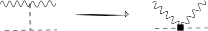
Figure 3: The $\sigma$ exchange channel. Double, dashed and wavy lines represent the $\sigma$-meson, pion and photon, respectively.

Consider for example $\sigma$-meson exchange. The relevant diagram is illustrated in Fig. 3. Effective interactions for $\sigma\gamma\gamma$ and $\sigma\pi\pi$ vertices can be written as

$$\mathcal{L}_{\sigma\gamma\gamma} = e^{2}\,g_{\sigma\gamma\gamma}\,F_{\mu\nu}F^{\mu\nu}\,\sigma,$$ (16)

$$\mathcal{L}_{\sigma\pi\pi} = g_{\sigma\pi\pi}\,\vec{\pi}\cdot\vec{\pi}\,\sigma\,.$$ (17)

According to the linear sigma model GellMann:1960np and the quark model calculation in Ref. Faessler:2003yf , the coefficients $g_{\sigma\pi\pi}$ and $g_{\sigma\gamma\gamma}$ can be written as

$$g_{\sigma\gamma\gamma}\approx\frac{5}{72\,\pi^{2}\,F_{\pi}},~{}~{}~{}~{}~{}g_{\sigma\pi\pi}=\frac{m_{\sigma}^{2}-M_{\pi}^{2}}{2\,F_{\pi}}\approx\frac{m_{\sigma}^{2}}{2\,F_{\pi}}.$$ (18)

With a simple calculation, one obtains a magnetic polarizability contribution of

$$\beta_{\pi}^{\sigma} = \frac{4\alpha}{M_{\pi}}\,\frac{g_{\sigma\gamma\gamma}\,g_{\sigma\pi\pi}}{m_{\sigma}^{2}}=\frac{5\alpha}{36\,\pi^{2}\,M_{\pi}\,F_{\pi}^{2}}=\frac{a_{-1}^{\sigma}}{M_{\pi}}\,,$$ (19)

thus generating a leading $1/{M_{\pi}}$ contribution to the $\pi^{0}$ magnetic polarizability at tree level with

$$a_{-1}^{\sigma}=4.7\times 10^{-4}\ \mbox{fm}^{2}\,.$$ (20)

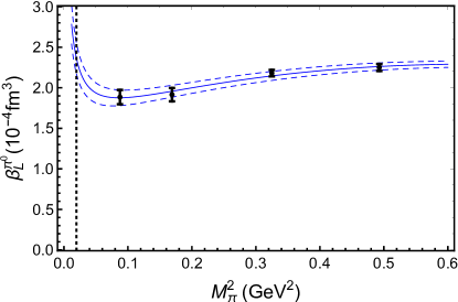
Figure 4: A description of lattice QCD results Bignell:2020dze (black points) for the magnetic polarizability of the neutral pion, $\beta^{\pi^{0}}_{L}$, in terms of the leading tree-level terms of chiral effective field theory. The solid curve indicates the fit and the dot-dashed curves indicate the uncertainty associated with the statistical uncertainties of the lattice results. The vertical dotted line indicates the physical point.

While the consideration of $\sigma$-meson exchange in this manner is somewhat phenomenological, its consideration admits a tree-level contribution proportional to $1/M_{\pi}$ that should be taken into account in fitting the results from lattice QCD calculations. In summary, the tree-level parameterization of Eq. (15) is used to describe the results of lattice QCD. The coefficients $a_{-1}$, $a_{1}$ and $a_{3}$ are determined by fitting results from lattice QCD Bignell:2020dze . With the lattice QCD results described, one can them proceed to include the missing contributions such as that of Eq. (13).

III Numerical Results

A description of the lattice QCD results obtained in Ref. Bignell:2020dze for the magnetic polarizability of the neutral pion, $\beta^{\pi^{0}}_{L}$, in terms of the leading tree-level terms of Eq. (15) is presented in Fig. 4. The lattice QCD results are described very well by the tree-level contributions. The parameters obtained in the fit are

$$a_{-1} = +1.34\times 10^{-4}fm^{2},$$ (21a)

$$a_{1} = +6.85\times 10^{-5}fm^{4},$$ (21b)

$$a_{3} = -1.22\times 10^{-6}fm^{6}\,.$$ (21c)

We note the leading coefficient is similar in scale to the model estimate of Eq. (20) but suggests $\sigma$ exchange contributions are smaller than estimated in the model.

With the fit parameters constrained, we can proceed to model the missing loop contributions associated with diagrams (e) through (h) of Fig. 2 and thus predict the full QCD result for $\beta_{\pi^{0}}$.

The correction to the leading coefficient, $a_{-1}$, is straight forward. As explained in the discussion of Fig. 2, the loop contribution of Fig. 1 cannot contribute in the contemporary lattice QCD results under consideration. Thus in correcting for the missing contribution, we draw on Eq. (13) and transform

$$a_{-1}\to a_{-1}+\frac{\alpha}{96\,\pi^{2}\,F_{\pi}^{2}}\,.$$ (22)

To correct $a_{1}$ we draw on the the two-loop chiral perturbation theory calculations of Refs. Bellucci et al. Bellucci:1994eb and more recently Gasser et al. Gasser:2005ud . At this order one obtains the same leading model-independent term from the one-loop contribution in Eq. (13). The two-loop contribution introduces terms at order $M_{\pi}$ and non-analytic terms involving $M_{\pi}\log M_{\pi}$ and $M_{\pi}\log^{2}M_{\pi}$ . The typical radius of convergence of chiral perturbation theory is $\sim 2M_{\pi}$, which means that it should be reasonable to draw from the two-loop expression of Ref. Gasser:2005ud to correct the magnetic polarizability at the physical pion mass.

Following the notation and associated values provided in Ref. Gasser:2005ud

$$\beta_{\rm 2loops}=\frac{\alpha}{32\,\pi^{2}\,F_{\pi}^{2}\,M_{\pi}}\left[\frac{1}{3}+\frac{M_{\pi}^{2}\,(d_{1+}-d_{1-})}{16\,\pi^{2}\,F_{\pi}^{2}}+{\cal O}(M_{\pi}^{4})\right]\,,$$ (23)

with

$$d_{1+} = 8\,b^{r}-\frac{1}{648}\,\left(144\,l\,(l+2\,\bar{l}_{2})\right.$$

$$\left.+96\,l+288\,\bar{l}_{2}+113+\Delta_{+}\right)\,,$$

$$d_{1-} = a_{1}^{r}+8\,b^{r}+\frac{1}{648}\,\left(144\,l\,(3\,\bar{l}_{\Delta}-1)\right.$$

$$\left.+36\,(8\,\bar{l}_{1}-3\,\bar{l}_{3}-12\,\bar{l}_{4}+12\,\bar{l}_{\Delta})+43+\Delta_{-}\right)\,,$$

$$\Delta_{+} = 13643-1395\,\pi^{2}\,,\quad\Delta_{-}=-3559+351\,\pi^{2}\,.$$ (24)

where $l\equiv\ln\left({M_{\pi}^{2}}/{\mu^{2}}\right),$ $\overline{l}_{i}$ are scale-independent low-energy couplings (LECs) defined in Eqs. (3.8) and (3.9) of Ref. Gasser:2005ud associated with divergences at order $p^{4}$ and, $a_{1}^{r}$ and $b^{r}$ are low-energy couplings associated with divergences at order $p^{6}$, defined in Eqs. (3.10) and (3.11) of Ref. Gasser:2005ud . The scale $\mu$ is taken to be the rho-meson mass, $\mu=M_{\rho}=0.770$ GeV. The uncertainty in the values of these parameters generates an uncertainty in the magnetic polarizability that will contribute in our systematic uncertainty analysis.

The contributions from the LECs of ${\mathcal{L}}_{6}$ contained in the coupling $a_{1}^{r}$ are associated with short-distance physics and therefore can have overlap with the lattice simulation results. We proceed by replacing the fit coefficient with the result from Eq. (23)

$$a_{1}\to\frac{\alpha}{2}\,\frac{-a_{1}^{r}}{\left(16\,\pi^{2}\,F_{\pi}^{2}\right)^{2}}\,.$$ (25)

The remaining logarithmic terms of Eq. (23) derived in the two-loop calculation are added. However, we also use these contributions as systematic uncertainty, both as a measure of the possible contributions from terms of higher-order in the chiral expansion and to account for any overlap with contributions already contained in the lattice QCD simulations. In summary, we model the full QCD magnetic polarizability of the neutral pion as

$$\beta_{\pi^{0}}^{\text{QCD}} = \left(a_{-1}+\frac{\alpha}{96\,\pi^{2}\,F_{\pi}^{2}}\right)\,\frac{1}{M_{\pi}}$$ (26)

$$+\frac{\alpha}{2}\,\frac{d_{1+}-d_{1-}}{\left(16\,\pi^{2}\,F_{\pi}^{2}\right)^{2}}\,M_{\pi}+a_{3}\,M_{\pi}^{3}\,.$$

The final full-QCD prediction for the magnetic polarizability of the neutral pion is shown in Fig. 5. There we show the original fit to the lattice QCD results and the full QCD prediction of Eq. (26) for $0\leq M_{\pi}^{2}\leq 2\,M_{\pi}^{2\,\rm Phys}$ where Eq. (26) is expected to display reasonable convergence.

Table 1 provides the contributions of terms considered in Eqs. (15) and (26). Here one observes the leading contribution of Eq. (26) dominates the full result. Similarly, the correction applied at order $M_{\pi}$ in Eq. (25) is relatively small.

Table 1: Contributions of terms considered in Eqs. (15) and (26) for the neutral pion magnetic polarizability in the standard units of $\times 10^{-4}$ fm³.

Description	Term	Value ($\times 10^{-4}$ fm3)
Full QCD Prediction	Eq. (26)	3.44
Leading term of Eq.(26)	$\displaystyle\left(a_{-1}+\frac{\alpha}{96\,\pi^{2}\,F_{\pi}^{2}}\right)\,\frac{1}{M_{\pi}}$	2.38
Leading one-loop contribution	$\displaystyle\frac{\alpha}{96\,\pi^{2}\,F_{\pi}^{2}}\,\frac{1}{M_{\pi}}$	0.50
Leading term of Eq. (15)	$\displaystyle a_{-1}\,\frac{1}{M_{\pi}}$	1.88
Order $M_{\pi}$ term of Eq.(26)	$\displaystyle\frac{\alpha}{2}\,\frac{d_{1+}-d_{1-}}{\left(16\,\pi^{2}\,F_{\pi}^{2}\right)^{2}}\,M_{\pi}$	1.06
Order $M_{\pi}$ correction of Eq. (25)	$\displaystyle\left(\frac{\alpha}{2}\,\frac{d_{1+}-d_{1-}}{\left(16\,\pi^{2}\,F_{\pi}^{2}\right)^{2}}-a_{1}\right)\,M_{\pi}$	0.58
Order $M_{\pi}^{3}$ term of Eq.(26)	$\displaystyle a_{3}\,M_{\pi}^{3}$	-0.004

At the physical pion mass, we find $\beta_{\pi^{0}}=3.44(19)(37)\times 10^{-4}$ fm³, where the first uncertainty tems from the statistical error from fitting the lattice QCD results and the second uncertainty is systematic as described above. The experimental value of $\beta_{\pi^{0}}^{\rm Expt}=1.29(1.10)\times 10^{-4}$ fm³ is from Ref. Filkov:1998rwz . It was determined by fitting the cross section for $\gamma\gamma\rightarrow\pi^{0}\pi^{0}$. Our prediction is just above the $1\sigma$ error bound of this experimental measurement.

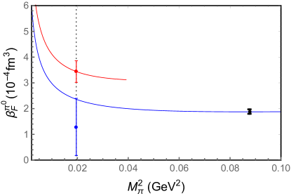
Figure 5: The full QCD prediction for the magnetic polarizability of the neutral pion $\beta_{\pi^{0}}$ (red curve). The previous fit (blue curve) of the lattice QCD simulation results (black points) has been corrected to incorporate pion-loop contributions absent in the current simulation results (red curve). The experimental measurement (blue point) and our corresponding prediction (red point) are plotted at the physical pion mass. Theoretical uncertainties include the statistical error from fitting the lattice QCD results and systematic uncertainties as described in the text.

IV Summary

In this paper, we have investigated the magnetic polarizability of the neutral pion based upon an analysis of recent lattice QCD simulations at a range of quark masses. The pion-photon scattering amplitude is first considered at the one-loop level in partially-quenched chiral perturbation theory. There, the structure of the four-pion vertex causes the sea-quark loop contributions to the magnetic polarizability at one loop to vanish. Thus the fact that the lattice simulations are electro-quenched has no impact on the leading one-loop-contributions to the magnetic polarizability.

The origin of the one-loop contributions is shown to be associated with the quark-annihilation contractions of the quark field operators of the neutral-pion interpolating fields. As these contributions have yet to be considered in lattice QCD, the results from contemporary calculations are associated with tree-level terms at this order.

By considering the relationship between the Compton amplitude and the magnetic polarizability a leading tree-level contribution proportional to $1/M_{\pi}$ was motivated, enabling a good characterisation of the lattice simulation results. The phenomenology of $\sigma$-meson exchange provides a specific model for generating such tree-level behavior.

The full QCD result is obtained by drawing on two-loop results from chiral perturbation theory. Because the lattice calculation does not include quark-annihilation loop contributions we are free to add the leading contribution from the two-loop result of chiral perturbation theory with no issue of double counting. While LEC contributions proportional to $M_{\pi}$ associated with short-distance physics are used to replace the lattice fit parameter, long-distance physics generating chiral logarithms are added to the lattice simulation results. Our final result is illustrated in Fig. 5.

Our prediction for the magnetic polarizability of the neutral pion is $\beta_{\pi^{0}}=3.44(19)^{\rm stat}(37)^{\rm syst}\times 10^{-4}$ fm³, just above the $1\sigma$ error bound of the experimental measurement. As the experimental uncertainty is reduced in future experiments we anticipate a significant increase in the central value.

Future research will focus on the inclusion of the quark-annihilation loop contributions in lattice QCD. As these results become available, our fit functions will be modified to include finite-volume effects and enable corrections to infinite volume. In this case no modeling of the leading contributions will be required, thus providing more robust predictions.

It will also be important to bring the techniques of partially-quenched chiral perturbation theory to the two-loop calculation to disclose the role of sea-quark loop contributions. While incorporating the effects of the quark charges in lattice QED+QCD simulations is now well established Borsanyi:2013lga ; Horsley:2015eaa , important correlations exploited in extracting the small energy shifts relevant to polarizabilities will be lost. This presents a formidable challenge to calculating sea-quark-loop contributions to magnetic polarizabilities from the first principles of QCD.

References

- (1) T. A. Aibergenov, P. S. Baranov, O. D. Beznisko, S. N. Cherepniya, L. V. Filkov, A. A. Nafikov, A. I. Osadchii, V. G. Raevsky, L. N. Shtarkov, and E. I. Tamm, “Radiative Photoproduction of Pions and Pion Compton Scattering,” Czech. J. Phys. B36 (1986) 948–951.
- (2) Yu. M. Antipov et al., “Measurement of pi- Meson Polarizability in Pion Compton Effect,” Phys. Lett. 121B (1983) 445–448.
- (3) Yu. M. Antipov et al., “Experimental Evaluation of the Sum of the Electric and Magnetic Polarizabilities of Pions,” Z. Phys. C26 (1985) 495.
- (4) J. Boyer et al., “Two photon production of pion pairs,” Phys. Rev. D42 (1990) 1350–1367.
- (5) Crystal Ball Collaboration, H. Marsiske et al., “A Measurement of Production in Two Photon Collisions,” Phys. Rev. D41 (1990) 3324.
- (6) L. V. Fil’kov and V. L. Kashevarov, “Determination of pi0 meson quadrupole polarizabilities from the process gamma gamma —¿ pi0 pi0,” Phys. Rev. C72 (2005) 035211, arXiv:nucl-th/0505058 [nucl-th].
- (7) V. Bernard and D. Vautherin, “Electromagnetic Polarizabilities of Pseudoscalar Goldstone Bosons,” Phys. Rev. D40 (1989) 1615.
- (8) M. A. Ivanov and T. Mizutani, “Pion and kaon polarizabilities in the quark confinement model,” Phys. Rev. D45 (1992) 1580–1601.
- (9) V. Bernard, A. A. Osipov, and U. G. Meissner, “Consistent treatment of the bosonized Nambu-Jona-Lasinio model,” Phys. Lett. B285 (1992) 119–125.
- (10) C. A. Wilmot and R. H. Lemmer, “Electric and magnetic polarizability of Goldstone pions to subleading O(Nc-1) in the bosonized Nambu-Jona-Lasinio model,” Phys. Rev. C65 (2002) 035206.
- (11) J. Bijnens and F. Cornet, “Two Pion Production in Photon-Photon Collisions,” Nucl. Phys. B296 (1988) 557–568.
- (12) S. Bellucci, J. Gasser, and M. Sainio, “Low-energy photon-photon collisions to two loop order,” Nucl. Phys. B 423 (1994) 80–122, arXiv:hep-ph/9401206. [Erratum: Nucl.Phys.B 431, 413–414 (1994)].
- (13) U. Burgi, “Charged pion pair production and pion polarizabilities to two loops,” Nucl. Phys. B479 (1996) 392–426, arXiv:hep-ph/9602429 [hep-ph].
- (14) J. Gasser, M. A. Ivanov, and M. E. Sainio, “Low-energy photon-photon collisions to two loops revisited,” Nucl. Phys. B728 (2005) 31–54, arXiv:hep-ph/0506265 [hep-ph].
- (15) M. Moinester and S. Scherer, “Compton Scattering off Pions and Electromagnetic Polarizabilities,” Int. J. Mod. Phys. A34 no. 16, (2019) 1930008, arXiv:1905.05640 [hep-ph].
- (16) L. V. Filkov, I. Guiasu, and E. E. Radescu, “Pion Polarizabilities From Backward and Fixed Sum Rules,” Phys. Rev. D26 (1982) 3146.
- (17) J. F. Donoghue and B. R. Holstein, “Photon-photon scattering, pion polarizability and chiral symmetry,” Phys. Rev. D48 (1993) 137–146, arXiv:hep-ph/9302203 [hep-ph].
- (18) V. Bernard, B. Hiller, and W. Weise, “Pion Electromagnetic Polarizability and Chiral Models,” Phys. Lett. B205 (1988) 16–21.
- (19) M. Burkardt, D. B. Leinweber, and X.-m. Jin, “Background field formalism in quantum systems,” Phys. Lett. B 385 (1996) 52–56, arXiv:hep-ph/9604450.
- (20) T. Primer, W. Kamleh, D. Leinweber, and M. Burkardt, “Magnetic properties of the nucleon in a uniform background field,” Phys. Rev. D 89 no. 3, (2014) 034508, arXiv:1307.1509 [hep-lat].
- (21) R. Bignell, J. Hall, W. Kamleh, D. Leinweber, and M. Burkardt, “Neutron magnetic polarizability with Landau mode operators,” Phys. Rev. D98 no. 3, (2018) 034504, arXiv:1804.06574 [hep-lat].
- (22) R. Bignell, W. Kamleh, and D. Leinweber, “Magnetic polarizability of the nucleon using a Laplacian mode projection,” Phys. Rev. D 101 no. 9, (2020) 094502, arXiv:2002.07915 [hep-lat].
- (23) E. Luschevskaya, O. Solovjeva, O. Kochetkov, and O. Teryaev, “Magnetic polarizabilities of light mesons in lattice gauge theory,” Nucl. Phys. B 898 (2015) 627–643, arXiv:1411.4284 [hep-lat].
- (24) E. Luschevskaya, O. Solovjeva, and O. Teryaev, “Magnetic polarizability of pion,” Phys. Lett. B 761 (2016) 393–398, arXiv:1511.09316 [hep-lat].
- (25) R. Bignell, W. Kamleh, and D. Leinweber, “Pion in a uniform background magnetic field with clover fermions,” Phys. Rev. D100 no. 11, (2020) 114518, arXiv:1910.14244 [hep-lat]. [Phys. Rev.D100,114518(2019)].
- (26) H.-T. Ding, S.-T. Li, A. Tomiya, X.-D. Wang, and Y. Zhang, “Chiral properties of (2+1)-flavor QCD in strong magnetic fields at zero temperature,” arXiv:2008.00493 [hep-lat].
- (27) R. Bignell, W. Kamleh, and D. Leinweber, “Pion magnetic polarisability using the background field method,” arXiv:2005.10453 [hep-lat].
- (28) J. M. M. Hall, D. B. Leinweber, and R. D. Young, “Finite-volume and partial quenching effects in the magnetic polarizability of the neutron,” Phys. Rev. D89 no. 5, (2014) 054511, arXiv:1312.5781 [hep-lat].
- (29) J. Hu, F.-J. Jiang, and B. C. Tiburzi, “Pion Polarizabilities and Volume Effects in Lattice QCD,” Phys. Rev. D 77 (2008) 014502, arXiv:0709.1955 [hep-lat].
- (30) C. W. Bernard and M. F. L. Golterman, “Chiral perturbation theory for the quenched approximation of QCD,” Phys. Rev. D46 (1992) 853–857, arXiv:hep-lat/9204007 [hep-lat].
- (31) D. B. Leinweber, “Quark contributions to baryon magnetic moments in full, quenched and partially quenched QCD,” Phys. Rev. D69 (2004) 014005, arXiv:hep-lat/0211017 [hep-lat].
- (32) M. Gell-Mann and M. Levy, “The axial vector current in beta decay,” Nuovo Cim. 16 (1960) 705.
- (33) A. Faessler, T. Gutsche, M. A. Ivanov, V. E. Lyubovitskij, and P. Wang, “Pion and sigma meson properties in a relativistic quark model,” Phys. Rev. D68 (2003) 014011, arXiv:hep-ph/0304031 [hep-ph].
- (34) L. V. Fil’kov and V. L. Kashevarov, “Compton scattering on the charged pion and the process gamma gamma —¿ pi0 pi0,” Eur. Phys. J. A5 (1999) 285–292, arXiv:nucl-th/9810074 [nucl-th].
- (35) Budapest-Marseille-Wuppertal Collaboration, S. Borsanyi et al., “Isospin splittings in the light baryon octet from lattice QCD and QED,” Phys. Rev. Lett. 111 no. 25, (2013) 252001, arXiv:1306.2287 [hep-lat].
- (36) R. Horsley et al., “Isospin splittings of meson and baryon masses from three-flavor lattice QCD + QED,” J. Phys. G 43 no. 10, (2016) 10LT02, arXiv:1508.06401 [hep-lat].