Coherent events at ion scales in the inner Heliosphere: Parker Solar Probe observations during the first Encounter

Abstract

Parker Solar Probe has shown the ubiquitous presence of strong magnetic field deflections, namely switchbacks, during its first perihelion where it was embedded in a highly Alfvénic slow stream. Here, we study the turbulent magnetic fluctuations around ion scales in three intervals characterized by a different switchback activity, identified by the behaviour of the magnetic field radial component, $B_{r}$. Quiet ($B_{r}$ does not show significant fluctuations), weak ($B_{r}$ has strong fluctuations but no reversals) and strong ($B_{r}$ has full reversals) periods show a different behaviour also for ion quantities and Alfvénicity. However, the spectral analysis shows that each stream is characterized by the typical Kolmogorov/Kraichnan power law in the inertial range, followed by a break around the characteristic ion scales. This frequency range is characterized by strong intermittent activity, with the presence of non-compressive coherent structures, such as current sheets and vortex-like structures, and wave packets, identified as ion cyclotron modes. Although, all these intermittent events have been detected in the three periods, they have a different influence in each of them. Current sheets are dominant in the strong period, wave packets are the most common in the quiet interval; while, in the weak period, a mixture of vortices and wave packets is observed. This work provides an insight into the heating problem in collisionless plasmas, fitting in the context of the new solar missions, and, especially for Solar Orbiter, which will allow an accurate magnetic connectivity analysis, to link the presence of different intermittent events to the source region.

1 Introduction

A puzzling aspect of the fast solar-wind dynamics consists in the empirical evidence that it is hotter than expected for an adiabatic expanding gas (Marsch et al., 1982; Lopez & Freeman, 1986; Freeman, 1988; Hellinger et al., 2013; Perrone et al., 2019a, b). Understanding the physical mechanisms of dissipation, and the related heating, in such a turbulent collision-free system, represents nowadays one of the key issues of plasma physics. Moreover, explaining how irreversible heating is accomplished represents a key challenge for thermodynamics in general, since any mechanism in which collisions are not present is lacking the part of the heating process related to the irreversible degradation of information (Pezzi et al., 2019; Matthaeus et al., 2020).

Spacecraft measurements generally reveal that the solar-wind plasma is in a state of fully-developed turbulence (Coleman, 1968; Bruno & Carbone, 2013). The energy injected by the Sun into the Heliosphere, in the form of large-wavelength fluctuations, e.g. Alfvén waves, is channeled towards short scales through a turbulent cascade until it can be eventually transferred to the plasma particles as heat (Kiyani et al., 2009; Alexandrova et al., 2009; Sahraoui et al., 2010). The magnetic power spectrum manifests, at scales corresponding to the inertial range, a behaviour reminiscent of the power-law that characterizes fluid turbulence (Kolmogorov, 1941; Tu & Marsch, 1995). Then, the turbulent cascade extends to smaller scales down to a wavelength range where ions become unmagnetized and the plasma dynamics is governed by particle kinetic properties. At these scales, around ion characteristic lengths, different physical processes come into play, leading to both changes in the spectral shape (Leamon et al., 1998; Bale et al., 2005; Alexandrova et al., 2013; Lion et al., 2016) and departure of the ion distribution functions from the thermodynamic equilibrium (Marsch, 2006; Servidio et al., 2015; Sorriso-Valvo et al., 2019).

Turbulence in the solar wind is strongly space-localized and the degree of non-homogeneity increases as the spatial scales decrease. This features, called intermittency and recovered in both magnetic field and plasma parameters (Veltri & Mangeney, 1999; Bruno et al., 2003; Salem et al., 2009; Bruno, 2019), has been observed to evolve with distance from the Sun and it is due to the presence of coherent structures (Bruno et al., 2003; Greco et al., 2012a), which can be described as strong non-homogeneities in the magnetic field (Retinò et al., 2007; Perri et al., 2012; Greco & Perri, 2014; Perrone et al., 2016, 2017) over a wide range of scales (Greco et al., 2016; Lion et al., 2016). Near these coherent structures, particle energization, temperature anisotropy, and strong deviation from Maxwellian have been observed in both in situ data and numerical simulations (Matteini et al., 2010; Osman et al., 2011; Greco et al., 2012b; Servidio et al., 2012, 2015, 2017; Wu et al., 2013; Perrone et al., 2013, 2014; Pezzi et al., 2018; Sorriso-Valvo et al., 2018).

Recently, a statistical study of coherent structures at ion scales has been performed in both slow (Perrone et al., 2016) and fast (Perrone et al., 2017) solar wind at $1$ au by using Cluster observations. It has been shown, for the first time, that different families of structures characterize the ion scales of the turbulent cascade of solar-wind plasma. This means that different mechanisms of dissipation occur at ion scales, since different structures interact with particles in different ways. Compressive structures, such as magnetic holes, solitons and shocks, and Alfvénic structures, in form of current sheets and vortices, are observed in slow solar wind (Perrone et al., 2016). In fast solar wind it has been found that the ion scales are dominated by Alfvén vortices, with a small and/or finite compressive part. Current sheets are also observed but no compressive structures are found (Perrone et al., 2017). In this respect, slow wind presents a more complex physics with respect to fast wind, where in the former a significant percentage of structures moves in the flow, maybe leading to the generation of instabilities with additional effects on particles (Hellinger et al., 2019).

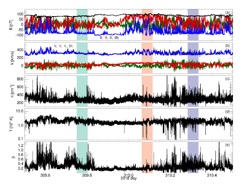
Figure 1: Overview of solar wind data during the first perihelion of Parker Solar Probe at $\sim 0.17$ au. From top to bottom: three components in RTN (radial in blue, tangential in red and normal in green) and magnitude (in black) of the magnetic (a) and velocity (b) field vectors; ion density (c) temperature (d), and plasma beta (e). The coloured bands denote three different periods, lasting 1h15, of quiet (green), weak (violet), and strong (orange) switchback activity.

A large variety of magnetic structures has also been detected in the inner heliosphere by using Messenger magnetic field observations at $0.3$ au (Greco & Perri, 2014) during the minimum of solar cycle 23. Unfortunately, due to the unavailability of the plasma data on the spacecraft, no information about the stream in terms of origin and/or speed is possible. However, by looking at magnetic field fluctuations, both Alfvénic, such as rotational and tangential discontinuties, and compressive structures, namely shocks and magnetic holes, have been identified. The study of the presence of coherent structures in the inner heliosphere, especially in regions close to the Sun, could help to explore the dynamical development of solar wind turbulence. Thanks to Parker Solar Probe (PSP, Fox et al., 2016), launched in August 2018, it is possible to study the presence and, eventually, the nature of coherent structures in a completely unexplored environment.

During its first perihelion, PSP revealed the presence of a large number of S-shaped magnetic structures which produce patches of large, intermittent magnetic field reversals, namely ‘switchbacks’ (Bale et al., 2019; Dudok de Wit et al., 2020), heat flux reversals and isolated intermittent velocity enhancements, namely ‘spikes’ (Kasper et al., 2019; Horbury et al., 2020). It is worth to remark that magnetic switchbacks have already been observed at different radial distances from the Sun by previous missions (Behannon & Burlaga, 1981; Tsurutani et al., 1994; Kahler et al., 1996; Balogh et al., 1999; Landi et al., 2006; Borovsky, 2016) but always in fast wind. Using PSP data, Krasnoselskikh et al. (2020) performed a detailed analysis on three selected structures, representative of three different groups of switchbacks, namely (i) Alfvénic-like structures, (ii) compressional-like structures, and (iii) full reversals of the radial component of the magnetic field vector. The size of these structures is large compared to the typical characteristic ion scales, except for their boundaries where flowing currents were found. Moreover, a rather intense wave activity, close to the edges of these structures has also been observed. This analysis suggests that these structures are localized twisted magnetic tubes moving with respect to the surrounding plasma.

Table 1: Typical solar wind parameters, averaged within each 1h15 selected period, observed by PSP at 0.17 au. Day and UT information refers to the starting time.

Period	Day	UT	$B$ [nT]	$V$ [km/s]	$n$ [cm${}^{-3}]$	$T$ [105K]	$\beta$	$V_{A}$ [km/s]	$\lambda_{i}$ [km]	$\rho_{i}$ [km]	$\Omega_{ci}$ [rad/s]
Quiet	309	18:14:24	84.3	312.2	301.1	1.9	0.28	106.0	12.1	6.9	8.1
Weak	310	06:47:31	85.6	311.4	331.2	2.0	0.32	102.6	12.5	7.0	8.2
Strong	310	01:29:17	99.5	344.8	306.1	1.8	0.19	124.0	13.0	5.6	9.5

In this paper, we study the nature of the turbulent magnetic fluctuations around ion scales in three PSP intervals with different characteristics during its first perihelion. In particular, by looking at the radial component of the magnetic field vector, $B_{r}$, we selected 1h15 intervals where (i) $B_{r}$ is almost constant, (ii) $B_{r}$ has strong fluctuations but no reversals, and (iii) $B_{r}$ has full reversals. In these three intervals, we focus on intermittency and we statistically study the observed coherent events. Examples of these events are also shown below.

The paper is organized as follows: in Section 2 we present the main characteristics of the first PSP encounter and we select the three intervals for the analysis; in Section 3 we show the results of statistical studies and we present examples of different coherent events; and in Section 4 we summarize the results and discuss our conclusions.

2 First PSP Encounter

In November 2018 PSP completed its first perihelion passage at about 0.17 au from the Sun, sampling the solar wind far closer than before. During this first encounter, the spacecraft was almost corotating with the Sun and observed a long interval of slow Alfvénic wind originating from a small equatorial coronal hole (Bale et al., 2019; Badman et al., 2020). These observations have shown the presence of isolated intermittent velocity enhancements (Kasper et al., 2019; Horbury et al., 2020) associated with magnetic field deflections (Bale et al., 2019; Dudok de Wit et al., 2020).

In this paper, we consider a one-day period (from 12:00 UT on 2018 November 5) around perihelion (see Figure 1) to study the nature of the turbulent magnetic fluctuations in three 1h15 intervals, with different characteristics in terms of switchbacks. We mainly focus on magnetic field measurements from the fluxgate Magnetometer (MAG), which is part of the FIELDS suite (Bale et al., 2016). We use the full cadence observations of the three components of the magnetic field vector, having a sampling rate of 293 Hz. Moreover, in order to set a context of the environment, we consider the solar wind bulk plasma properties measured by the Solar Probe Cup (SPC, Case et al., 2020), a solar-facing Faraday cup, from the SWEAP instrument suite (Kasper et al., 2016). The ion density, $n$, and velocity, ${\bf V}$, are derived by taking moments of the one-dimensional ion velocity distribution obtained by the current spectra, the primary data product of the SPC sensor, with a cadence of about 0.87 s. The ion temperature, $T$, is also estimated from the ion thermal speed, $v_{th}$, which is also a regular derived product of SPC, as $T=mv_{th}^{2}/2k_{B}$, being $m$ the proton mass and $k_{B}$ the Boltzmann’s constant.

2.1 Intervals Characterization

In Figure 1, an overview of the solar wind in the considered one-day period around the first perihelion of PSP is summarized, where magnetic field data have been downsampled to comply with the resolution of particle measurements. Panels (a) and (b) show the three components in RTN reference frame (radial in blue, tangential in red and normal in green) and magnitude (in black) of the magnetic and velocity field vectors, respectively. It is clear, especially looking at the radial component of the magnetic field vector, that different regimes lie in this one-day interval, where the switchback activity significantly varies. In particular, we observe periods where $B_{r}$ is almost constant and periods where $B_{r}$ has strong fluctuations and sometimes fully reverses. Therefore, we decided to separately perform our studies on three 1h15 selected periods, denoted in Figure 1 by coloured bands. From now on, we will refer to quiet (green band), weak (violet band) and strong (orange band) periods if $B_{r}$ does not show significant fluctuations, $B_{r}$ has strong fluctuations but no reversals and $B_{r}$ has full reversals, respectively. Panels (c) and (d) display the ion density and temperature, respectively. Differences are also recovered in these quantities with respect to the three selected periods. In particular, the largest fluctuations around a mean value are found in the weak interval, while in the strong one a change in the behaviour is observed in correspondence of the reversals. Finally, in panel (e), we show the ion plasma beta, $\beta$, defined as the ratio between ion kinetic and magnetic pressures. Also in this case, we found the same features observed for the density.

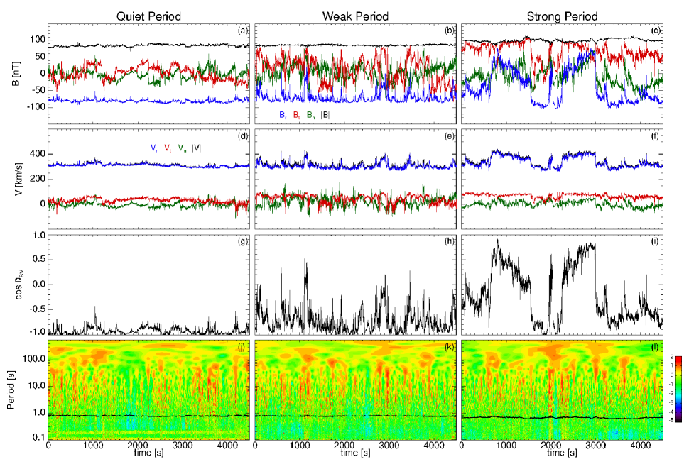
Figure 2: Characteristics of the quiet (left column), weak (middle column), and strong (right column) periods. From top to bottom: zoom of Figure 1 in the selected intervals for the magnetic (first row) and velocity (second row) field vectors; cosine of the angle between the magnetic and velocity field vectors (third row); logarithmic contour plots of the Local Intermittency Measure (LIM) of the total magnetic field fluctuations (fourth row). In the latter, black lines denote the ion cyclotron timescale.

Looking at the typical solar-wind parameters (listed in Table 1), averaged within each selected interval considered in this study, we observe that quiet and weak periods have almost the same values of the magnitude of the magnetic and velocity field vectors, while in the strong period higher values are found. The same trend is observed for the characteristic derived quantities, such as the Alfvén speed, $V_{A}$, the ion Larmor radius, $\rho_{i}$, and the ion cyclotron frequency, $\Omega_{ci}$. Moreover, we see that the ion density is larger for the weak period, probably due to the presence of stronger fluctuations, while the temperature and the ion skin depth, $\lambda_{i}$, have similar values in all the three intervals. Finally, the ion plasma beta is lower in the strong period ($\beta\sim 0.19$), while is higher in the weak interval ($\beta\sim 0.32$).

In Figure 2, we look more in detail at the three periods. The first two rows are just a zoom of Figure 1 in the selected intervals for the magnetic and velocity field vectors, respectively. Here, we can better appreciate the behaviour of $B_{r}$: in the quiet (a) period it is almost constant, in the weak (b) period it undergoes short scale variations, and in the strong (c) period it largely rotates. Moreover, quiet (a) and weak (b) periods have almost constant magnetic field magnitude, while $B$ in the strong period (c) is more variable. Furthermore, for the velocity field vector, we observed an increase of spikes in $V_{r}$ for the weak (e) and strong (f) intervals with respect to the quiet one (d). Finally, the $V_{r}$ component is highly correlated with $B_{r}$ in all the three periods, which of course indicates a high level of Alfvénicity in the wind. To better stress this aspect, we also plot the cosine of the angle between ${\bf B}$ and ${\bf V}$ (third row). The quiet period shows a very high degree of Alfvénicity, with anti-parallel magnetic and velocity field vectors (g). Lower Alfvénicity is found in both weak (h) and strong (i) intervals, even if we can recognize that the change in sign follows the fluctuations of the magnetic field.

The last row of Figure 2 shows the Local Intermittency Measure (LIM, Farge, 1992) for the total magnetic field fluctuations, $|\mathcal{W_{\bf B}}(\tau,t)|^{2}=\sum_{i}|\mathcal{W}_{i}(\tau,t)|^{2}$ with $i=r,t,n$, defined as

$$I(\tau,t)=\frac{|\mathcal{W_{\bf B}}(\tau,t)|^{2}}{\langle|\mathcal{W_{\bf B}}(\tau,t)|^{2}\rangle_{t}}$$ (1)

where the brackets indicate a time average and $\mathcal{W}_{i}(\tau,t)$ are the Morlet wavelet coefficients for different timescales $\tau$ and time $t$ (Torrence & Combo, 1998)

$$\mathcal{W}_{i}(\tau,t)=\sum_{j=0}^{N-1}B_{i}(t_{j})\psi^{*}\left[\left(t_{j}-t\right)/\tau\right]\ .$$ (2)

Black lines denote the local ion cyclotron timescale. In all the three intervals, the distribution of energy in time and scales (not affected by edge effects) is not uniform, with the appearance of localized energetic events covering a certain range of scales, which are easily recognized by the red color. This is an indication of the presence of coherent structures in the system which emerge at larger time scales and are connected through the scales (Perrone et al., 2016, 2017; Lion et al., 2016; Alexandrova et al., 2020). Similar features have also been reported by Greco et al. (2016) using the partial variance of increments technique. In panels (j)–(l), we can also observe that sometimes the energy appears localized around the ion characteristic scales (see, e.g., the energy appearing after $t=1000$ s in panel (k) around the inverse of the ion cyclotron frequency). This would suggest the localized presence of some wave activity (Alexandrova et al., 2004; Lion et al., 2016; Bowen et al., 2020).

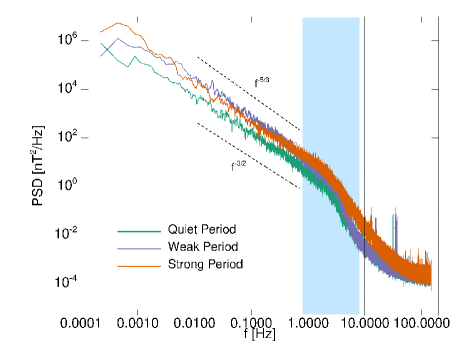
Figure 3: Power Spectral Density (PSD) of the total magnetic field fluctuations for the quiet (green), weak (violet), and strong (orange) periods. Both Kolmogorov and Kraichnan scalings (black dotted lines) have been plotted for reference. The vertical black solid line indicates the maximum resolved frequency for the spectra ($f_{max}=10$ Hz), while the blue filled band denotes the range of scales, $f\in[0.8,8]$ Hz, around ion scales.

Figure 3 shows the total power spectral density (i.e. the trace of the spectral matrix) of the magnetic field for the quiet (green), weak (violet) and strong (orange) periods. The vertical solid line at $f=10$ Hz indicates the frequency at which the noise level becomes significant. These spectra show the characteristic behaviour of the solar wind turbulent cascade. For each stream, we observe at low frequencies a power-law trend between the Kolmogorov (Kolmogorov, 1941) and the Kraichnan (Kraichnan, 1965) scaling (black dotted lines). Indeed, in the inertial range, in the frequency range $f\in[0.016,0.8]$ Hz, the spectral indices for the quiet, weak and strong intervals are $-1.548\pm 0.015$, $-1.759\pm 0.014$, and $-1.487\pm 0.013$, respectively. These values are in agreements with the results described in Chen et al. (2020) and Duan et al. (2020). Then, a break between the inertial range and the dissipative range of the turbulent cascade can be identified around ion scales. The frequency location of the break for each time interval, which is around 2 and 3 Hz, has been estimated adopting the same procedure described in Bruno & Trenchi (2014), closer to the prediction based on the ion cyclotron resonance mechanism (Leamon et al., 1998), in agreement with previous studies (Leamon et al., 1998; Bruno & Trenchi, 2014; Woodham et al., 2018; D’Amicis et al., 2019; Duan et al., 2020). In particular, for the three different time intervals, quiet, weak and strong, we obtain the following ion cyclotron resonance frequencies: $2.49$ Hz, $2.53$ Hz and $2.95$ Hz, respectively, considering that the ion cyclotron frequency is, for the three intervals, 1.29 Hz, 1.30 Hz and 1.51 Hz. To compare, both Doppler shifted ion Larmor radius and inertia length can be estimated, under the assumption of wave vectors parallel to the plasma flow, by using the information in Table 1. Indeed, we found $f_{\lambda_{i}}\simeq 3.8$ Hz, $4$ Hz, $4.2$ Hz and $f_{\rho_{i}}\simeq 7.2$ Hz, $7.1$ Hz, $9.8$ Hz, for quiet, weak and strong interval, respectively.

For the present study we are interested in the investigation of the nature of the turbulent fluctuations around ion scales, indicated in Figure 3 by the blue filled band. Therefore, from now on, our analysis will focus on the denoted range of scales $f\in[0.8,8]$ Hz.

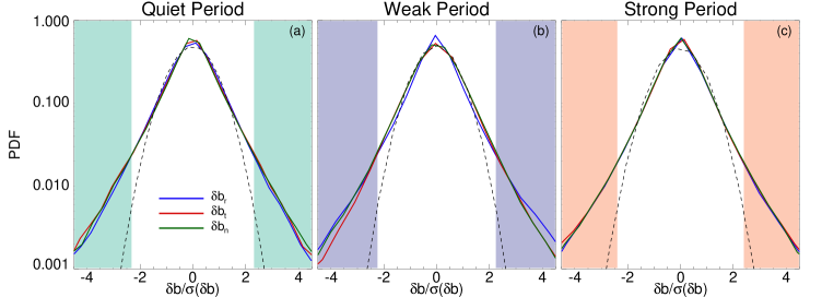
Figure 4: Probability distribution functions (PDFs) of $\delta b_{r}$ (blue), $\delta b_{t}$ (red), and $\delta b_{n}$ (green), normalized to their own standard deviations, $\sigma(\delta b_{i})$, for the quiet (a), weak (b), and strong (c) periods. In each panel, black dashed lines, correspond to a Gaussian fit and the filled bands show the regions where magnetic fluctuations exceed three standard deviations of each Gaussian fit.

3 Coherent structures

In order to look at the overall nature of the magnetic field fluctuations in the chosen range of scales, we adopt a bandpass filter based on the wavelet transform (Torrence & Combo, 1998; He et al., 2012; Roberts et al., 2013; Perrone et al., 2016, 2017). The fluctuations are defined as

$$\delta b_{i}(t)=\frac{\delta j\delta t^{1/2}}{C_{\delta}\psi_{0}(0)}\sum_{j=j_{1}}^{j_{2}}\frac{\mathcal{R}\left[\mathcal{W}_{i}(\tau_{j},t)\right]}{\tau_{j}^{1/2}}$$ (3)

where $\mathcal{R}$ refers to the real-part function, $j$ is the scale index and $\delta j$ is the constant scale step; $\psi_{0}(0)=\pi^{1/4}$ and $C_{\delta}=0.776$, the latter derived from the reconstruction of a $\delta$ function using the Morlet wavelet (Torrence & Combo, 1998). Finally, $\tau(j_{1})=0.125$ s and $\tau(j_{2})=1.25$ s (being $\tau=1/f$).

In Figure 4, we show the probability distribution functions (PDFs) of the three components of the magnetic field fluctuations ($\delta b_{r}$ in blue, $\delta b_{t}$ in red, and $\delta b_{n}$ in green), normalized to their own standard deviation, $\sigma(\delta b_{i})$, for the quiet (a), weak (b) and strong (c) intervals. By comparing the PDFs with a Gaussian fit (black dashed line), we observe the presence of significant non-Gaussian tails in each component of the magnetic field fluctuations, due to the presence of strong energetic events (Perrone et al., 2016, 2017). This result is confirmed by the flatness of the magnetic fluctuations, which has the same behavior in the three periods analyzed (not shown). We find that the flatness departs from the normal distribution value around the ion scales, showing an almost flat curve around 4.9, 5.2 and 5.4 for quiet, weak and strong intervals, respectively. This reflects a non-homogeneous distribution of the turbulent fluctuations in all the three periods. In each panels of Figure 4, the filled bands show the regions where magnetic fluctuations exceed three standard deviations of the corresponding Gaussian fit, which include $99.7\%$ of the Gaussian contribution. We will use the corresponding value in each period as a threshold to select non-Gaussian intermittent events. More than thousand events have been detected in each period, thus supporting a statistical analysis of their properties.

3.1 Statistical Analysis

Figure 5 shows the results of the minimum variance analysis (Sonnerup & Scheible, 1998) applied to the intermittent events observed in the quiet (green), weak (violet), and strong (orange) periods. It is worth pointing out that this analysis has been performed around each selected peak in magnetic energy, which identifies magnetic fluctuations well-localized in time and with regular profiles, in a defined time range, $\Delta t^{{}^{\prime}}$, between two minima of energy. This corresponds to the width (i.e. extension) of an event, larger than its characteristic temporal scale, $\Delta t$, which is defined as the width at half height (see Perrone et al., 2016, for more details on the identification method for intermittent events).

The left column displays the histograms for the minimum, $\lambda_{min}$ (a) and intermediate, $\lambda_{int}$ (b) eigenvalues normalized to the maximum eigenvalue, $\lambda_{max}$, and for $\lambda_{min}/\lambda_{int}$ (c). Although most of the considered events, in all the intervals, have $\lambda_{min}\ll\lambda_{int}\ll\lambda_{max}$, we also find the presence of fluctuations with $\lambda_{min}\ll\lambda_{int}\lesssim\lambda_{max}$, a feature a bit more pronounced in the quiet period. In general, the minimum variance direction is well defined in all the three considered periods, even if for a very few events, a degeneracy $\lambda_{min}\sim\lambda_{int}$ exists.

The right column shows the histograms of the orientation of the eigenvectors with respect to the local magnetic field, ${\bf b}_{0}$, also averaged within the structure, thus in $\Delta t^{{}^{\prime}}$. The direction of maximum variation, $\theta_{max}$ (d), is perpendicular to ${\bf b}_{0}$ in all the three intervals, suggesting the absence of compressive events. Differences between the periods, instead, are found in the distributions of $\theta_{int}$ (e) and $\theta_{min}$ (f). In particular, we observe in the quiet period an almost uniform distribution for both $\theta_{int}$ and $\theta_{min}$, while in the weak and strong intervals $\theta_{int}$ is peaked around $90^{\circ}$ and $\theta_{min}$ is almost parallel to ${\bf b}_{0}$.

To better highlight the differences between the three intervals with respect to the intermittent events observed, in Figure 6 we show the histograms of $\beta$ (a), $\theta_{BV}$ (b), and $\zeta_{\parallel}$ (c), being the latter the local magnetic compressibility (Perrone et al., 2016), defined as

where parallel and perpendicular directions are evaluated with respect to ${\bf b}_{0}$ and the maximum of the magnetic components is evaluated within $\Delta t^{{}^{\prime}}$; while $\beta$ and $\theta_{BV}$ have been evaluated as mean values in the same time range. The distribution of the ion plasma beta displays three distinct peaks, which reflects the behaviour of $\beta$ in the whole three periods (see Table 1), i.e. the largest value is found for the events in the weak interval and the lowest for the ones in the strong period. Three distinct peaks are also recovered for the angle between the magnetic and velocity field vectors in each event, where $\theta_{BV}\sim 20^{\circ}$ for the quiet interval (green line), $30^{\circ}<\theta_{BV}<50^{\circ}$ for the weak period (violet line), and $\theta_{BV}\sim 90^{\circ}$ for the strong one (orange line). This behaviour suggests that the disalignment of ${\bf b}_{0}$ and ${\bf v}_{0}$ increases as the switchback activity increases. It is worth pointing out that the value of $\theta_{BV}$ gives a view of the plasma wave vectors that we are able to measure. In particular, for $\theta_{BV}\sim 0^{\circ}$ $k_{\parallel}$ are well measured, while for $\theta_{BV}\sim 90^{\circ}$ $k_{\perp}$ turbulence is observed. An opposite behaviour with respect to $\theta_{BV}$, is observed, even if less marked, for the local magnetic compressibility (see Figure 6c). Finally, the distribution of the characteristic time scale of these events, $\Delta t$, in all the three periods, is peaked at about $0.25$ s (not shown), which corresponds to $\sim 0.3$–$0.4$ ion cyclotron timescale or, by assuming that the frozen-in, Taylor hypothesis is fulfilled (Perri et al., 2017) to a spatial scale of $\sim 6$–$7$ $\lambda_{i}$ or $\sim 11$–$15$ $\rho_{i}$.

3.2 Examples of Observed Coherent Events

A detailed analysis of all the events observed in the selected periods has allowed us to identify three different families of intermittent events, all of them present in the three periods, namely (i) current sheets, (ii) vortex-like structures, and (iii) wave packets. Examples are shown in Figure 7. The top row displays the modulus of the raw magnetic field, i.e. the large-scale magnetic field as observed by PSP, where we have only taken off the noise for $f>10$ Hz. The three panels have the same aspect ratio to highlight the magnetic compressibility of the events. Middle and bottom rows show the magnetic field fluctuations, as defined in Equation 3, in the minimum variance reference frame (MVRF) and in the local magnetic field reference frame where ${\bf b_{0}}$ is along the $z$-direction (${\bf e_{z}}={\bf e_{b}}$), $x$ is perpendicular to ${\bf b_{0}}$ in the plane spanned by it and the radial direction (${\bf e_{x}}={\bf e_{b}}\times{\bf e_{b}}$), and $y$ closes the right-hand reference frame (${\bf e_{y}}={\bf e_{b}}\times{\bf e_{x}})$, respectively. Finally, vertical dashed lines mark the width of the events, $\Delta t^{{}^{\prime}}$, where all the analyses have been performed.

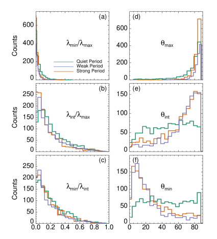
Figure 5: Statistical analysis of the observed coherent events in the minimum variance reference frame for the quiet (green), weak (violet), and strong (orange) periods. Left panels: histograms for the minimum (a) and intermediate (b) eigenvalues normalized to the maximum eigenvalue, and for $\lambda_{min}/\lambda_{int}$ (c). Right panels: histograms of the angles between the maximum (d), intermediate (e), and minimum (f) variance directions and the local magnetic field.

The first example of intermittent event is a current sheet (left column), an incompressible one-dimensional (i.e. linearly polarized) structure, with $\delta b_{x}$ (g), perpendicular to ${\bf b}_{0}$, which changes sign. The other two components show very small fluctuations. Moreover, the three components are almost zero in the middle of the structure, where $\delta b_{max}$ reverses (d) and the large-scale magnetic field has a local minimum (a). Finally, the minimum variance analysis shows that the direction of maximum variation is perpendicular to ${\bf b}_{0}$, with $\theta_{max}\simeq 85^{\circ}$.

The second example (middle column) suggests the presence of an Alfvén vortex (Alexandrova et al., 2006; Alexandrova, 2008; Roberts et al., 2016; Lion et al., 2016; Perrone et al., 2017; Wang et al., 2019). The large-scale magnetic field shows a modulated fluctuation with a local maximum in the middle of the structure (b). The fluctuations are localized, with the main variation in the direction perpendicular to ${\bf b}_{0}$, $\delta b_{x}$ (h). Indeed, from the minimum variance analysis, we found that the maximum variance is perpendicular to the local magnetic field, $\theta_{max}\simeq 87^{\circ}$, while $\theta_{int}\simeq 10^{\circ}$ and $\theta_{min}\simeq 80^{\circ}$. In the case of a vortex, as we suppose here, where $\lambda_{int}\simeq\lambda_{min}$, the direction of minimum variance corresponds to the normal direction, while the direction of intermediate variance, which is parallel to the local magnetic field, corresponds to the vortex axis.

The last example (right column) has no a clear behaviour in the large-scale magnetic field (c), but $\delta b_{i}$ show quasi-monochromatic magnetic fluctuations from $-6$ to $6$ nT, in the plane perpendicular to ${\bf b}_{0}$ (i). The minimum variance analysis gives $\theta_{max}\simeq 86^{\circ}$ and $\theta_{int}\simeq 85^{\circ}$, while the minimum variance direction is almost parallel, $\theta_{min}\simeq 6^{\circ}$. We also note that the transverse components are out of phase of about $\pi/2$. The observed features can be associated to a wave activity.

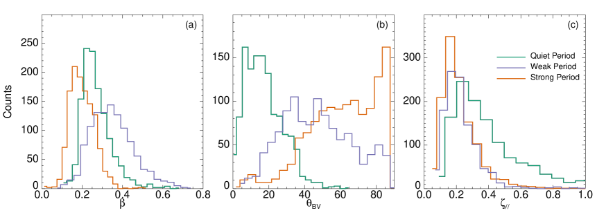
Figure 6: Histograms of $\beta$ (a), $\theta_{BV}$(b), and $\zeta_{\parallel}$ (c), for the observed coherent events in the quiet (green), weak (violet), and strong (orange) periods.

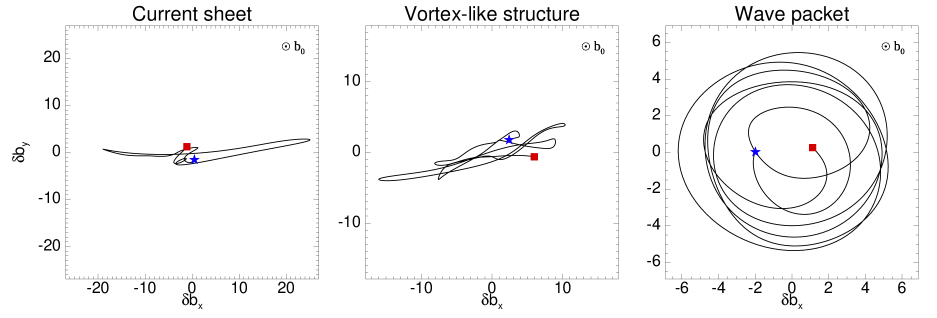
Figure 8: Hodogram for the magnetic field fluctuations of the current sheet (left), vortex-like structure (middle) and wave packet (right) shown in Figure 7, in the plane perpendicular to the local ${\bf b_{0}}$. Blue star refers to the starting time point and red square to the end time point.

To better highlight the polarization of these events, in Figure 8 we show the hodograms for the components of the magnetic field fluctuations in the plane perpendicular to the local magnetic field (with the local magnetic field direction out of plane) for the examples of current sheet (left), vortex-like structure (middle) and wave packet (right) shown in Figure 7. Blue star indicates the starting point, while the red square the end one for the magnetic temporal signal. The first two hodograms confirm the linear polarization of both the current sheet and the vortex-like structure. Such linear polarisation for vortices can be found while crossing the vortex very close to its centre (see e.g. Alexandrova & Saur, 2008). On the other hand, the fluctuations of the wave packet are clearly left-handed circularly polarized around the direction of ${\bf b_{0}}$, which is inward directed, and can be interpreted as outward propagating ion cyclotron waves (He et al., 2011; Podesta & Gary, 2011; Telloni et al., 2015). This is in agreement with the results in Huang et al. (2020). Ion cyclotron waves are indeed left-handed polarized waves, with a wavevector nearly aligned to the local magnetic field and frequencies around the proton gyrofrequency. In solar wind, they can be found in individual wave packets lasting a few minutes (Jian et al., 2009; Lion et al., 2016; Bowen et al., 2020) or in ‘storms’ lasting many hours (Jian et al., 2010, 2014; Wicks et al., 2016; Lion, 2016; Bowen et al., 2020). Their presence has also been found in numerical simulations (Pezzi et al., 2017). Ion cyclotron waves have recently been directly observed in the solar wind in periods characterized by strong Alfvénic fluctuations at inertial scales (see Telloni et al., 2019, and references therein).

4 Discussions

We have studied in detail the nature of magnetic turbulent fluctuations around the ion characteristic scales in the inner heliosphere, by using the unique opportunity offered by PSP which is sampling the solar wind far closer than ever before. In particular, we focused on a one-day interval around its first perihelion, at 0.17 au, where we selected three 1h15 periods characterized by a different switchback activity (looking at the behaviour of $B_{r}$), and we studied magnetic properties at ion scales, thus smaller than the ones considered in Krasnoselskikh et al. (2020).

The three chosen intervals, namely quiet ($B_{r}$ does not show significant fluctuations), weak ($B_{r}$ has strong fluctuations but no reversals) and strong ($B_{r}$ displays full reversals), show different characteristics also in terms of large-scale plasma quantities. In particular, stronger fluctuations, in both density and temperature, are found for the whole weak interval, while in the strong one reversals drive changes in their behaviour. Moreover, we observed an increase of the presence of spikes in $V_{r}$ for the weak and strong intervals, with respect to the quiet period. Furthermore, the magnitude of both the velocity and magnetic field vectors are the same in the quiet and weak periods, with an almost constant trend, but becomes larger, and with small changes, in the strong interval. Finally, differences are observed also for the Alfvénicity, which is very strong in the quiet interval, while is lower in both weak and strong periods. It is worth pointing out that, for turbulent fluctuations at the scales considered in this work, the angle between magnetic and velocity field vectors also indicates which wave vectors are observed. Indeed, if $\theta_{BV}\sim 0^{\circ}$ or $\theta_{BV}\sim 180^{\circ}$, the satellite is able to scan $k_{\parallel}$, while for oblique angles $k_{\perp}$ turbulence is well measured. In this study, $k_{\parallel}$ is mostly resolved in the quiet period, while in the other two intervals $\theta_{BV}$ covers all possible angles, meaning that both $k_{\parallel}$ and $k_{\perp}$ can be measured.

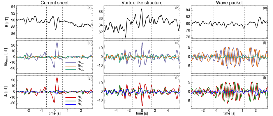
Figure 7: Example of current sheet (left column), vortex-like structure (middle column), and wave packet (right column). Top row: magnitude of the large-scale magnetic field. Middle row: components of the magnetic field fluctuations, defined in Equation 3, in the minimum variance frame. The maximum direction is in violet, the intermediate in orange and the minimum in green. Bottom row: components of the magnetic field fluctuations in the local magnetic field reference frame, where ${\bf b_{0}}$ is along the $z$-direction. The vertical black dashed lines mark the extension of the events, $\Delta t^{{}^{\prime}}$.

The study of the spectral properties for the three considered periods showed that each stream is characterized, in the inertial range, by a power law between the Kolmogorov spectrum and the Kraichnan scaling. Then a break, around the characteristic ion scales has been observed. In addition, the frequency break location seems to match the one predicted by the ion cyclotron resonance mechanism, confirming previous results based on different s/c observations (Bruno & Trenchi, 2014; Woodham et al., 2018; D’Amicis et al., 2019; Duan et al., 2020). Moreover, we also looked at the distribution of the magnetic energy in time and frequency and we found that localized regions in time that cover a certain range of scales exist in all the considered intervals. We also observed that sometimes energy appears localized around the ion cyclotron frequency. This kind of non-homogeneity in the magnetic energy distribution has already been observed in both slow and fast wind at 1 au and it has been related to the presence, at ion scales, of different families of coherent structures or waves (Alexandrova et al., 2004; Lion et al., 2016; Perrone et al., 2016, 2017). Motivated by these results, we decided to study magnetic fluctuations in the range $f\in[0.8,8]$ Hz, around the typical ion scales for these intervals, which are also characterized by a significant departure from Gaussianity.

We have detected more than thousand intermittent events in each period, which have well-localized fluctuations in space with regular profiles. These events can be divided in three different families, namely current sheets, vortex-like structures, and wave packets, with different influence in each considered period. A minimum variance analysis has shown that the peak of the distributions for the eigenvalues is found for $\lambda_{min}\ll\lambda_{int}\ll\lambda_{max}$, meaning a prevalence of one-dimensional fluctuations. This is the case, for example, of the current sheets, which are the most common events in the strong period ($\sim 46\%$ out of $\sim 220$ events for which the magnetic profile is clear). However, also two-dimensional fluctuations are found, where $\lambda_{int}\lesssim\lambda_{max}$. In particular, values of $\lambda_{int}/\lambda_{max}\in[0.2,0.6]$ can be recovered in case of vortices, while $\lambda_{int}\simeq\lambda_{max}$ can be found for the case of wave packets. In the weak period we observe a mixture of vortices ($\sim 45\%$ out of $\sim 342$) and wave packets ($\sim 50\%$), while in the quiet period, where $\theta_{BV}\sim 0^{\circ}$ allowing to resolve $k_{\parallel}$ waves (Lion, 2016; Bowen et al., 2020), wave packets are the most frequent class of intermittent events ($\sim 61\%$ out of $\sim 303$). The left-handed circular polarization around the direction of the local magnetic field of these wave packets suggests that these wave modes can correspond to ion cyclotron waves. Evidence for the presence of ion cyclotron waves in highly Alfvénic periods supports previous findings by Telloni et al. (2019, 2020), where a clear link between the Alfvénicity at fluid scales and the existence of ion cyclotron waves at kinetic scales has statistically been proved. Moreover, ion cyclotron waves are associated to high levels of temperature anisotropy, which lead the proton velocity distribution to depart from thermodynamic equilibrium, thus triggering the development of proton cyclotron plasma instability (see e.g. Gary et al., 1994; Bourouaine et al., 2010; Telloni et al., 2019).

The minimum variance analysis has also shown that the direction of maximum variation is, in all the three intervals, perpendicular to the local magnetic field, suggesting the absence of compressive events. This is in disagreement with the results in slow wind at 1 au (Perrone et al., 2016); however, the slow wind observed by PSP is highly Alfvénic, with much more similarities with the fast wind (D’Amicis et al., 2019; Stansby et al., 2020; Perrone et al., 2020; Telloni et al., 2020). In fact, we found a good agreement, for the distribution of $\theta_{max}$ and $\theta_{min}$ in the quiet period, with the observations in fast wind at 1 au (Perrone et al., 2017). In particular, in the quiet interval we found an almost uniform distribution for both $\theta_{int}$ and $\theta_{min}$, suggesting that the presence of vortices ($\sim 31\%$), jointly with waves (the dominant contribution), could generate a mix-up of the intermediate and minimum directions, thus all possible angle can be covered. Finally, the very low magnetic compressibility found in our analysis is also in agreement with the results in the inner heliosphere, using Helios data in fast solar wind (Bavassano et al., 1982).

Understanding the role of small-scale coherent structures and waves into the general problem of dissipation, and thus heating, in collisionless plasmas, and especially in solar wind, represents a key problem for space plasma physics. In situ measurements (Marsch, 2006; Bourouaine et al., 2010; Wu et al., 2013) and numerical experiments (Araneda et al., 2008; Valentini et al., 2008; Perrone et al., 2013, 2014) have shown that particle heating and acceleration and temperature anisotropy appear localized in and near coherent structures or due to wave-particle interactions. Unfortunately, the resolution of the particle measurements on PSP is not enough to study in details the kinetics within the selected events (the mean width of the events is around 2 s and the resolutions for ion data is about 1 s). However, some indications can be obtained. In particular, peaks of both ion density and temperature are noticed at the edges of both current sheets and vortex-like structures (not shown). Conversely, we saw a peak within wave packets for both ion density and temperature (not shown).

The new observations of these macroscopic magnetic switchbacks made by PSP are allowing to add new pieces to the puzzle of the energy dissipation mechanisms in collisionless plasmas. However, the origin of such structures remains still unclear and debated. Until now, several physical processes, both in-situ (Squire et al., 2020; Ruffolo et al., 2020) and in the solar atmosphere (see for instance Tenerani et al., 2020), have been proposed to explain these switchbacks. Among the many possibilities, it was pointed out that these could be due to coronal jets and filament eruptions (Sterling & Moore, 2020), to reconnection processes or to phenomena happening in the deep corona. It has been shown, through state-of-the-art numerical modelling (Tenerani et al., 2020), that these perturbations may indeed originate in the solar atmosphere and propagate upwards. In this regard, it is worth recalling that large amplitude kink-like oscillations are nowadays detected in small-scale magnetic elements at all heights in the solar atmosphere, from the corona and chromospheric heights (see for instance Anfinogentov et al., 2013; Jafarzadeh et al., 2017, to mention a few) down to the photosphere, where they are excited by the forcing action of the granular buffeting (Stangalini et al., 2014). In the near future, thanks to the synergy between PSP, which will collect measurements far closer to the Sun, and Solar Orbiter (Mullet et al., 2013), which will combine both remote sensing and in situ measurements, it will be possible to provide further insights in the understanding the link between the switchbacks in the solar wind and their possible source in the solar atmosphere.

References

- Alexandrova et al. (2004) Alexandrova, O., Mangeney, A., Maksimovic, M., et al. 2004, J. Geophys. Res. 109, A05207
- Alexandrova et al. (2006) Alexandrova, O., Mangeney, A., Maksimovic, M., et al. 2004, J. Geophys. Res. 111, A12208
- Alexandrova (2008) Alexandrova, O. 2008, Nonlinear Proc. Geophys. 15, 95
- Alexandrova & Saur (2008) Alexandrova, O., & Saur, J. 2008, Geophys. Res. Lett. 35, L15102
- Alexandrova et al. (2009) Alexandrova, O., Saur, J., Lacombe, C., et al. 2009, Phys. Rev. Lett. 103, 165003
- Alexandrova et al. (2013) Alexandrova, O., Chen, C. H. K., Sorriso-Valvo, L., Horbury, T. S., & Bale, S. D. 2013, Space Sci. Rev. 178, 101
- Alexandrova et al. (2020) Alexandrova, O., Jagarlamudi, V., Rossi, C., et al. 2020, submitted to Nature Communications, https://arxiv.org/abs/2004.01102
- Anfinogentov et al. (2013) Anfinogentov, S., Nisticò, G., & Nakariakov, V. M. 2013, A&A 560, A107
- Araneda et al. (2008) Araneda, J. A., Marsch, E., & Viñas, A. F. 2008, Phys. Rev. Lett. 100, 125003
- Badman et al. (2020) Badman, S. T., Bale, S. D., Martínez Oliveros, J. C., et al. 2020, Astrophys. J. Supplement Series 246, 23
- Bale et al. (2005) Bale, S. D., Kellogg, P. J., Mozer, F. S., Horbury, T. S., & Reme, H. 2005, Phys. Rev. Lett. 94, 215002
- Bale et al. (2016) Bale, S. D., Goetz, K., Harvey, P. R., et al. 2016, Space Sci. Rev. 204, 49
- Bale et al. (2019) Bale, S. D., Badman, S. T., Bonnell, J. W., et al. 2019, Nature 576, 237
- Balogh et al. (1999) Balogh, A., Forsyth, R. J., Lucek, E. A., Horbury, T.S., & Smith, E. J. 1999, Geophys. Res. Lett. 26, 631
- Bavassano et al. (1982) Bavassano, B., Dobrowolny, M., Fanfani, G., Mariani, F., & Ness, N. F. 1982, Solar Phys. 78, 373
- Behannon & Burlaga (1981) Behannon, K. W., & L. F. Burlaga 1981, in Solar Wind 4, ed. H. Rosenbauer (Garching: Max-Planck-Institute für Aeronomie), 374
- Borovsky (2016) Borovsky, J. E. 2016, J. Geophys. Res. 121, 5055
- Bourouaine et al. (2010) Bourouaine, S., Marsch, E., & Neubauer, F. M. 2010, Geophys. Res. Lett. 37, L14104
- Bowen et al. (2020) Bowen, T. A., Mallet, A., Huang, J., et al. 2020, Astrophys. J. Supplement Series 246, 66
- Bruno et al. (2003) Bruno, R., Carbone, V., Sorriso-Valvo, L., & Bavassano, B. 2003, J. Geophys. Res. 108, A3, 1130
- Bruno & Carbone (2013) Bruno, R., & V. Carbone 2013, Living Rev. Sol. Phys. 10, 2
- Bruno & Trenchi (2014) Bruno, R., & L. Trenchi 2014, Astrophys. J. Lett. 787, L24
- Bruno (2019) Bruno, R. 2019, Earth and Space Science 6, 656
- Case et al. (2020) Case, A. C., Kasper, J. C., Stevens, M. L., et al. 2020, Astrophys. J. Supplement Series 246, 43
- Chen et al. (2020) Chen, C. H. K., Bale, S. D., Bonnell, J. W., et al. 2020, Astrophys. J. Supplement Series 246, 53
- Coleman (1968) Coleman, P. J. Jr 1968, Astrophys. J. 153, 371
- D’Amicis et al. (2019) D’Amicis, R., Matteini, L., & Bruno, R. 2019, MNRAS 483, 4665
- Duan et al. (2020) Duan, D., Browen, T. A., Chen, C. H. K., et al. 2020, Astrophys. J. Supplement Series 246, 55
- Dudok de Wit et al. (2020) Dudok de Wit, T., Krasnoselskikh, V. V., Bale, S. D., et al. 2020, Astrophys. J. Supplement Series 246, 39
- Farge (1992) Farge, M. 1992, Ann. Rev. Fluid Mech. 24, 395
- Fox et al. (2016) Fox, N. J., Velli, M., Bale, S. D., et al. 2016, Space Sci. Rev. 204, 7
- Freeman (1988) Freeman, J. W. 1988, Geophys. Res. Lett. 15, 88
- Gary et al. (1994) Gary, S. P., McKean, M. E., Winske, D., et al. 1994, J. Geophys. Res. 99, 5903
- Greco et al. (2012a) Greco, A.,Matthaeus, W. H., D’Amicis, R., Servidio, S., Dmitruk, P. 2012a, Astrophys. J. 749, 105
- Greco et al. (2012b) Greco, A., Valentini, F., Matthaeus, W. H., Servidio, S., Dmitruk, P. 2012b, Phys. Rev. E 86, 066405
- Greco & Perri (2014) Greco, A., & Perri, S. 2014, Astrophys. J. 784, 163
- Greco et al. (2016) Greco, A., Perri, S., Servidio, S., Yordanova, E., & Veltri, P. 2016, Astrophys. J. Lett. 823, L39
- He et al. (2011) He, J., Marsch, E., Tu, C., Yao, S., & Tian, H. 2011, Astrophys. J. 731, 85
- He et al. (2012) He, J., Tu, C., Marsch, E., & Yao, S. 2012, Astrophys. J. Lett. 745, L8
- Hellinger et al. (2013) Hellinger, P., Trávnícek, P. M., Stverák, S., Matteini, L., & Velli, M. 2013, J. Geophys. Res. 118, 1351
- Hellinger et al. (2019) Hellinger P., Matteini L., Landi S., et al. 2010, Astrophys. J. 883, 178
- Horbury et al. (2020) Horbury, T. S., Woolley, T., Laker, R., et al. 2020, Astrophys. J. Supplement Series 246, 45
- Huang et al. (2020) Huang, S. Y., Zhang, J., Sahraoui, F., et al. 2020, Astrophys. J. Lett. 897, L3
- Jafarzadeh et al. (2017) Jafarzadeh, S., Solanki, S. K., Stangalini, M., et al. 2017, Astrophys. J. Supplement Series 229, 1
- Jian et al. (2009) Jian, L. K., Russell, C. T., Luhmann, J. G., et al. 2009, Astrophys. J. Lett. 701, L105
- Jian et al. (2010) Jian, L. K., Russell, C. T., Luhmann, J. G., et al. 2010, J. Geophys. Res. 115, A12115
- Jian et al. (2014) Jian, L. K., Wei, H. Y., Russell, C. T., et al. 2014, Astrophys. J. 786, 123
- Kahler et al. (1996) Kahler, S. W., Crocker, N. U., & Gosling, J. T. 1996, J. Geophys. Res. 101, 24373
- Kasper et al. (2016) Kasper, J. C., Abiad, R., Austin, G., et al. 2016, Space Sci. Rev. 204, 131
- Kasper et al. (2019) Kasper, J. C., Bale, S. D., Belcher, J. W., et al. 2019, Nature 576, 228
- Kiyani et al. (2009) Kiyani, K. H., Chapman, S. C., Khotyaintsev, Yu. V., Dunlop, M. W., & Sahraoui, F. 2009, Phys. Rev. Lett. 103, 075006
- Kolmogorov (1941) Kolmogorov, A. 1941, Dokl. Akad. Nauk SSSR 30, 9
- Kraichnan (1965) Kraichnan, R. H. 1965, Phys. Fluids 8, 1385
- Krasnoselskikh et al. (2020) Krasnoselskikh, V., Larosa, A., Agapitov, O., et al. 2020, Astrophys. J. 893, 93
- Landi et al. (2006) Landi, S., Hellinger, P., & Velli, M. 2006, Geophys. Res. Lett. 33, L14101
- Leamon et al. (1998) Leamon, R. J., Matthaeus, W. H., Smith, C. W., & Wong, H. K. 1998, Astrophys. J. Lett. 507, L181
- Lion et al. (2016) Lion, S., Alexandrova, O., & Zaslavsky, A. 2016, Astrophys. J. 824, 47
- Lion (2016) S. Lion 2016, Analyse multi-satellite et multi-échelle de la turbulence dans le vent solaire. Astrophysique [astro-ph]. Université Pierre et Marie Curie - Paris VI, https://tel.archives-ouvertes.fr/tel-01478328
- Lopez & Freeman (1986) Lopez, R. E., & J. W. Freeman 1986, J. Geophys. Res. 91, A2, 1701
- Marsch et al. (1982) Marsch, E., Muhlhauser K.-H., Schwenn R., Rosenbauer H., Pilipp W., & Neubauer F. M. 1982, J. Geophys. Res. 87, A1, 52
- Marsch (2006) Marsch, E. 2006, Living Rev. Sol. Phys. 3, 1
- Matteini et al. (2010) Matteini, L., Landi, S., Velli, M., & Hellinger, P. 2010, J. Geophys. Res. 115, A09106
- Matthaeus et al. (2020) Matthaeus W. H., Yang Y., Wan M., et al. 2020, Astrophys. J. 891, 101
- Mullet et al. (2013) Muller, D., Marsden, R. G., St. Cyr, O. C., et al. 2013, Solar Phys. 283, 25
- Osman et al. (2011) Osman, K. T., Matthaeus, W. H., Greco, A., & Servidio, S. 2011, Astrophys. J. Lett. 727, L11
- Perri et al. (2012) Perri, S., Carbone, V., Vecchio, A., Bruno, R., Korth, H., Zurbuchen, T. H., & Sorriso-Valvo, L. 2012, Phys. Rev. Lett. 109, 245004
- Perri et al. (2017) Perri, S., Servidio, S., Vaivads, A., & Valentini, F. 2017, Astrophys. J. Supplement Series 231, 4
- Perrone et al. (2011) Perrone, D., Valentini, F. & Veltri, P. 2001, Astrophys. J. 741, 43
- Perrone et al. (2013) Perrone, D., Valentini, F., Servidio, S., Dalena, S., & Veltri, P. 2013, Astrophys. J. 762, 99
- Perrone et al. (2014) Perrone, D., Valentini, F., Servidio, S., Dalena, S., & Veltri, P. 2014, Eur. Phys. J. D68, 209
- Perrone et al. (2016) Perrone, D., Alexandrova, O., Mangeney, A., et al. 2016, Astrophys. J. 826, 196
- Perrone et al. (2017) Perrone, D., Alexandrova, O., Roberts, O. W., et al. 2017, Astrophys. J. 849, 49
- Perrone et al. (2019a) Perrone, D., Stansby, D., Horbury, T.S, & Matteini, L. 2019, MNRAS 483, 3730
- Perrone et al. (2019b) Perrone, D., Stansby, D., Horbury, T.S, & Matteini, L. 2019, MNRAS 488, 2380
- Perrone et al. (2020) Perrone, D., D’Amicis, R., De Marco, R., et al. 2020, A&A 633, A166
- Pezzi et al. (2017) Pezzi, O., Malara, F., Servidio, S., et al. 2017, Phys. Rev. E 96, 023201.
- Pezzi et al. (2018) Pezzi, O., Servidio, S., Perrone, D., et al. 2018, Phys. Plasmas 25, 060704
- Pezzi et al. (2019) Pezzi, O., Perrone, D., Servidio, S., et al. 2019, Astrophys. J. 887, 208
- Podesta & Gary (2011) Podesta, J. J., & Gary, S. P. 2011, Astrophys. J. 734, 15
- Retinò et al. (2007) Retinò, A., Sundkvist, D., Vaivads, A., et al. 2007, Nature Phys. 3, 235
- Roberts et al. (2013) Roberts, O. W., Li, X., & Li, B. 2013, Astrophys. J. 769, 58
- Roberts et al. (2016) Roberts, O. W., Li, X., Alexandrova, O., & Li, B. 2016, J. Geophys. Res. 121, 3870
- Ruffolo et al. (2020) Ruffolo, D. Matthaeus, W. H., Chhiber, R., et al. 2020, https://arxiv.org/abs/2009.06537
- Sahraoui et al. (2010) Sahraoui, F., Goldstein, M. L., Belmont, G., Canu, P., & Rezeau, L. 2010, Phys. Rev. Lett. 105, 131101
- Salem et al. (2009) Salem, C., Mangeney, A., Bale, S. D., & Veltri, P. 2009, Astrophys. J. 702, 537
- Servidio et al. (2012) Servidio, S., Valentini, F., Califano, F., & Veltri, P. 2012, Phys. Rev. Lett. 108, 045001
- Servidio et al. (2015) Servidio, S., Valentini, F., Perrone, D., et al. 2015, J. Plasma Phys. 81, 325810107
- Servidio et al. (2017) Servidio, S., Chasapis, A., Matthaeus, W. H., et al. 2017, Phys. Rev. Lett. 119, 205101
- Sonnerup & Scheible (1998) Sonnerup, B., & M. Scheible 1998, Analysis Methods for Multi-Spacecraft Data, The Netherlands:ESA Publ. Div.
- Sorriso-Valvo et al. (2018) Sorriso-Valvo, L., Perrone, D., Pezzi, O., et al. 2018, J. Plasma Phys. 84, 725840201
- Sorriso-Valvo et al. (2019) Sorriso-Valvo, L., Catapano, F., Retinò, A., et al. 2019, Phys. Rev. Lett. 122, 035102
- Squire et al. (2020) Squire, J., Chandran, B. D. G., & Meyrand, R. 2020, Astrophys. J. Lett. 891, L2
- Stangalini et al. (2014) Stangalini, M., Consolini, G., Berrilli, F., De Michelis, P., & Tozzi, R. 2014, A&A 569, A102
- Stansby et al. (2020) Stansby, D., Matteini, L., & Horbury, T. S. 2020, MNRAS 492, 39
- Sterling & Moore (2020) Sterling, A. C., & R. L. Moore 2020, Astrophys. J. Lett. 896, L18
- Telloni et al. (2015) Telloni, D., Bruno, R., & Trenchi, L. 2015, Astrophys. J. 805, 46
- Telloni et al. (2019) Telloni, D., Carbone, F., Bruno, R., et al. 2019, Astrophys. J. Lett. 885, L5
- Telloni et al. (2020) Telloni, D., D’Amicis, R., Bruno, R., et al. 2020 Astrophys. J. 897, 167
- Tenerani et al. (2020) Tenerani, A., Velli , M., Matteini, L., et al. 2020, Astrophys. J. Supplement Series 246, 32
- Torrence & Combo (1998) Torrence, C., & Combo, G. P. 1998, Bulletin of the American Meteorological Society 79, 61
- Tsurutani et al. (1994) Tsurutani, B. T., Ho, C. M., Smith, E. J., et al. 1994, Geophys. Res. Lett. 21, 2267
- Tu & Marsch (1995) Tu, C.-Y., & E. Marsch 1995, Space. Sci. Rev. 73, 1
- Valentini et al. (2008) Valentini, F., Veltri, P., Califano, F., & Mangeney, A. 2008, Phys. Rev. Lett. 101, 025006
- Veltri & Mangeney (1999) Veltri, P., & Mangeney, A. 1999, AIP Conf. Proc. 471, 543
- Wang et al. (2019) Wang, T., Alexandrova, O., Perrone, D., et al. 2019, Astrophys. J. Lett. 871, L22
- Wicks et al. (2016) Wicks, R. T., Alexander, R. L., Stevens, M., et al., Astrophys. J. 819, 6
- Woodham et al. (2018) Woodham, L. D., Wicks, R. T., Verscharen, D., & Owen, C. J. 2018, Astrophys. J. 856, 49
- Wu et al. (2013) Wu, P., Perri, S., Osman, K., et al. 2013, Astrophys. J. Lett. 763, L30