Analytic charged BHs in $f(R)$ gravity

Abstract

In this article, we seek exact charged spherically symmetric black holes (BHs) with considering $f(R)$ gravitational theory. This BH is characterized by convolution and error functions. Those two functions depend on a constant of integration which is responsible to make such a solution deviate from Einstein’s general relativity (GR). The error function which constitutes the charge potential of the Maxwell field depends on the constant of integration and when this constant is vanishing we cannot reproduce the Reissner-Nordström BH in the lower order of $f(R)$. This means that we cannot reproduce Reissner-Nordström BH in lower-order-curvature theory, i.e., in GR limit $f(R)=R$, we cannot get the well known charged BH. We study the physical properties of these BHs and show that it is asymptotically approached as a flat spacetime or approach AdS/dS spacetime. Also, we calculate the invariants of the BHS and show that the singularities are milder than those of BHs in GR. Additionally, we derive the stability condition through the use of geodesic deviation. Moreover, we study the thermodynamics of our BH and show the effect of the higher-order-curvature theory. Finally, we study the stability analysis by using the odd-type mode and show that all the BHs are stable and have radial speed equal to one.

I Introduction

Despite the simplicity, elegantly and powerfully of GR, which is considered as a classical theory, and despite its successes in the prediction of the shadow of BH, which confirmed by horizon telescope Akiyama et al. (2019a, b); Ayzenberg and Yunes (2018), and its success with observation, like the bending of light, perihelion precession of mercury, the gravitational redshift of radiation from distant stars Will (2005, 2006); Yunes and Siemens (2013), it has unsolved problems. Among these issues, is the problem of dark energy and dark matter which confirmed by recent observation Milgrom (1983); Bekenstein and Milgrom (1984); Milgrom and Sanders (2003); Perlmutter et al. (1999); Riess et al. (1998), the problem of singularities Penrose (1965); Hawking (1976); Christodoulou (1991), the problem of quantum gravity Rovelli (1996); Ashtekar et al. (2006). All these issues make physicists demand another theory that is eligible and able to overcome such problems and permit GR in the lower energy. Therefore, a satiate modified gravitational theory has been constructed that can overcome the issues that GR cannot solve. Later, physicists put constraints that any modified gravity must bypass like: its consistency with the solar system, free from ghost modes, able to describe the observations in which GR could not solve, and must not create a fifth force in local physics. There are many modified theories that satisfy such benchmark and are categorized as:

• Theories in which their Lagrangian involve higher-order curvature like $f(R)$, Nojiri and Odintsov (2011); Capozziello et al. (2006), Lanczos-Lovelock models Lanczos (1932, 1938); Lovelock (1971); Padmanabhan and Kothawala (2013); Dadhich et al. (2016) etc.

• Higher-dimensional theories which change the equation of motions of 4-dimension because of the higher-order correction of the energy-momentum tensor Shiromizu et al. (2000); Awad and Nashed (2017); Harko and Mak (2004); Carames et al. (2013); Haghani et al. (2012); Chakraborty and SenGupta (2015).

• Scalar theories of gravity like Brans-Dicke theory and the more general Horndeski models Brans and Dicke (1961); Horndeski (1974); Sotiriou and Zhou (2014); Babichev et al. (2016).

In this study, we take $f(R)$ gravitational theory which is considered as the excellent modification of the Einstein GR at the most recent time. Among many things that make $f(R)$ gravity be the best modification of GR is its simplified Lagrangian which contains an arbitrary function whose lowest order coincides with Einstein’s theory. The $f(R)$ gravity is an elegant theory to describe an expanded accelerated universe which is supported from recent observations Riess et al. (2004, 1998). Moreover, it is supposed that a special form of $f(R)$ can mimic some curvature modifications that come from the quantum theory of gravity. The justifications of invented modified theories of GR are to construct complete systems of gravitational models to cure the issues appearing in GR. These systems are considered in various topics of gravity like astrophysics, cosmology and the output of these studies construct as a suitable extension of the Einstein GR Cognola et al. (2005); Cooney et al. (2010); Guo and Frolov (2013). Recently, the $f(R)$ gravity theory gains much attentions which generalize the gravitational Lagrangian of GR Sotiriou and Faraoni (2010); Hendi (2010); Capozziello and De Laurentis (2011); Maeda (1989). There are two methods to obtain the equation of motions of $f(R)$ gravitational theory, the first through the use of metric structure and the other through the use of the Palatini method in which the connection and metric are taken as independent variables Antoniadis et al. (2020). There are many viable applications of $f(R)$ in the domain of cosmology as well as astrophysics Amendola et al. (2007); Li and Barrow (2009); Hu and Sawicki (2007); Starobinsky (2007) and in a specific case, $f(R)$ can reduce to GR case Capozziello et al. (2016).

There are many spherically symmetric BH solutions derived in $f(R)$ Multamäki and Vilja (2006); Nashed (2018a, b, 2002, 2018). Moreover, novel spherically symmetric BH solutions have been obtained in the context of $f(R)$ Elizalde et al. (2020); Nashed et al. (2019); Nashed and Capozziello (2019). It is well known that higher-order curvature terms play an ingredient role in strong gravitational background in local objects of $f(R)$. In this context, many physicists concentrate on the study of spherically symmetric BHs Sultana and Kazanas (2018); Cañate (2018); Nashed (2010); Yu et al. (2018); Cañate et al. (2016); Kehagias et al. (2015); Nelson (2010); de la Cruz-Dombriz et al. (2009). This exposition aims to derive original spherically symmetric charged BH solutions in $f(R)$ gravity devoid of any constraints on the form of $f(R)$ nor the Ricci scalar and study their contingent physics. In the frame of $f(R)$-gravity, a Lagrangian approach has been developed to study dynamics of spherically symmetric metrics. The Euler-Lagrange equations are obtained and solved in the case of constant curvature $R=R_{0}$ recovering the standard Schwarzschild-de Sitter solution of GR Capozziello et al. (2012).

The paper is structured as: In Sec. II, we give a brief construction of $f(R)$ gravity. In Sec. III, we employ the charged equation of motions of $f(R)$ to a spherically symmetric spacetime having two unknown metric potentials and derive a system of non-linear differential equations. These systems have four unknown functions, two of the metric potentials, one from the gauge potential of the charge and the derivative of $f(R)$. To be able to solve this system and to put it in a closed system, we assume a form of the derivative of $f(R)$, which depends on a constant of integration and solve the system. The BH solution is characterized by convolution and error functions and they become constant functions when the constant of integration that appears in the derivative function of $f(R)$ is equal to zero and in that case, we have a GR BHs. Therefore, the convolution and error functions appear like the effect of higher-order curvature that characterizes $f(R)$ gravity. Moreover, we study the physics of these BHs by giving the asymptote form of the convolution and error functions up to certain order and showing the effect of the higher-order curvature. We examine the singularities of the BHs by calculating the invariants of the Kretschmann scalar, the Ricci tensor square, and the Ricci scalar and investigate the effect of higher-order curvature on these invariants by showing that the singularity of our BHs is milder than the GR BHs. Also in Sec. III, we calculate the geodesic deviation and give the condition of stability. In Sec. IV, we show the validity of the first law of thermodynamics and also calculate some thermodynamic quantities like the Hawking temperature, entropy, the Gibbs free energy, and quasi-local energy of these BHs. We reserve the final section for the discussion and conclusion of this study.

II Fundamentals of $f(R)$ gravitational theory

We are going to study a 4-dimensional Lagrangian of $f(R)$ with $f$ being an arbitrary function. The Lagrangian of $f(R)$ is given by (cf. Carroll et al. (2004); Buchdahl (1970); Nojiri and Odintsov (2003); Capozziello et al. (2003); Capozziello and De Laurentis (2011); Nojiri and Odintsov (2011); Nojiri et al. (2017); Capozziello (2002)):

$${\mathop{\mathcal{L}}}:=\frac{1}{2\kappa}\int d^{4}x\sqrt{-g}\leavevmode\nobreak\ f(R)+\int d^{4}x\leavevmode\nobreak\ \sqrt{-g}\leavevmode\nobreak\ \mathcal{L}_{\mathrm{em}}\,.$$ (1)

Here $\kappa$ and $g$ are the Newtonian gravitational constant and the determinant of the metric. The Lagrangian of electromagnetic field $\mathcal{L}_{\mathrm{em}}$ is defined as $\mathcal{L}_{\mathrm{em}}={F}$ where ${F}=d{\xi}$ and ${\xi}={\xi}_{\beta}dx^{\beta}$ is the electromagnetic Maxwell gauge potential 1-form Capozziello et al. (2013).

Making the variations principle w.r.t. the metric tensor $g_{\alpha\beta}$ to the Lagrangian (1) we get the equation of motions of $f(R)$ gravitational theory in the form Cognola et al. (2005)

$${\mathop{\mathcal{I}}}_{\mu\nu}={R}_{\mu\nu}f_{R}-\frac{1}{2}g_{\mu\nu}f(R)+\left[g_{\mu\nu}\Box-\nabla_{\mu}\nabla_{\nu}\right]f_{R}+\frac{1}{2}\kappa{T_{\mathrm{(em)}}}_{\mu\nu}\equiv 0\,,$$ (2)

with $\Box$ being the d’Alembertian operator, $\displaystyle f_{R}=\frac{d{f}}{{d{R}}}$, and ${T_{\mathrm{(em)}}}^{\nu}_{\mu}$ is the energy-momentum tensor of the Maxwell field defined as

$${T_{\mathrm{(em)}}}^{\ \nu}_{\mu}={F}_{\mu\alpha}{F}^{\nu\alpha}-\frac{1}{4}\delta_{\mu}^{\ \nu}{F}\,,$$ (3)

where ${F}={F}_{\mu\nu}{F}^{\mu\nu}$. Moreover, the variation of Eq. (1) w.r.t. the gauge potential 1-form, ${\xi}_{\mu}$, gives:

$$\partial_{\alpha}\left(\sqrt{-g}{F}^{\mu\nu}\right)=0\,.$$ (4)

The trace of the field equations  (2), takes the form:

$${\mathop{\mathcal{E}}}=3\Box f_{R}+Rf_{R}-2f(R)\equiv 0\,.$$ (5)

From Eq. (5) one can obtain $f(R)$ in the form:

$$f(R)=\frac{1}{2}\left[3\Box f_{R}+Rf_{R}\right]\,.$$ (6)

Using Eq. (6) in Eq. (2) we get Kalita and Mukhopadhyay (2019)

$$I_{\mu\nu}=R_{\mu\nu}f_{R}-\frac{1}{4}g_{\mu\nu}Rf_{R}+\frac{1}{4}g_{\mu\nu}\Box f_{R}-\nabla_{\mu}\nabla_{\nu}f_{R}+\frac{1}{2}\kappa{T_{\mathrm{(em)}}}_{\mu\nu}=0\,.$$ (7)

We will apply the field equations (5), (7), and (3) to a spherically symmetric spacetime with two unequal unknown functions in the next section.

III Spherically symmetric black hole solutions

Let us take the following line-element

$$ds^{2}=-\mu(r)dt^{2}+\frac{dr^{2}}{\nu(r)}+r^{2}\left(d\theta^{2}+\sin^{2}d\phi^{2}\right)\,,$$ (8)

which describes a spherically symmetric a spacetime with $\mu(r)$ and $\nu(r)$ which are two functions of the radial coordinate $r$ to be determined from the equation of motions. From Eq. (8), the Ricci scalar takes the form:

$${R}(r)=\frac{r^{2}\nu\mu^{\prime 2}-r^{2}\mu\mu^{\prime}\nu^{\prime}-2r^{2}\mu\nu\mu^{\prime\prime}-4r\mu[\nu\mu^{\prime}-\mu\nu^{\prime}]+4\mu^{2}(1-\nu)}{2r^{2}\mu^{2}}\,,$$ (9)

where $\mu\equiv\mu(r)$, $\nu\equiv\nu(r)$, $\mu^{\prime}=\frac{d\mu}{dr}$, $\mu^{\prime\prime}=\frac{d2\mu}{dr^{2}}$, and $\nu^{\prime}=\frac{d\nu}{dr}$. Applying the equation of motions (4), (5) and (7) to the line-element (8) using Eq. (9), we get the following non-linear differential equations:

$${\mathop{\mathcal{I}}}_{t}{}^{t}= \frac{1}{8r^{2}\alpha^{2}}\left\{r^{2}\left[\nu{F}_{1}\alpha^{\prime 2}-3\alpha{F}_{1}\nu^{\prime}\alpha^{\prime}-2\alpha\nu{F}_{1}\alpha^{\prime\prime}-2\alpha^{2}{F}_{1}\nu^{\prime\prime}-3\alpha\nu\alpha^{\prime}{F}^{\prime}_{1}-2\alpha^{2}\nu^{\prime}{F}^{\prime}_{1}+2\nu\alpha^{2}{F}^{\prime}_{1}\right]\right.$$

$$\left.-4r\alpha\nu\left[{F}_{1}\alpha^{\prime}-\alpha{F}^{\prime}_{1}\right]-4\alpha^{2}{F}_{1}\left[1-\nu\right]^{\prime}-8\alpha r^{2}{\xi}^{\prime 2}\right\}=0\,,$$

$${\mathop{\mathcal{I}}}_{r}{}^{r}= \frac{1}{8r^{2}\alpha^{2}}\left\{r^{2}\left[\nu{F}_{1}\alpha^{\prime 2}-3\alpha{F}_{1}\nu^{\prime}\alpha^{\prime}-2\alpha\nu{F}_{1}\alpha^{\prime\prime}-2\alpha^{2}{F}_{1}\nu^{\prime\prime}+\alpha\nu\alpha^{\prime}{F}^{\prime}_{1}-2\alpha^{2}\nu^{\prime}{F}^{\prime}_{1}-6\nu\alpha^{2}{F}^{\prime\prime}_{1}\right]\right.$$

$$\left.+4r\alpha\nu\left[{F}_{1}\alpha^{\prime}+\alpha{F}^{\prime}_{1}\right]-4\alpha^{2}{F}_{1}\left[1-\nu\right]-8\alpha r^{2}{\xi}^{\prime 2}\right\}=0\,,$$

$${\mathop{\mathcal{I}}}_{\theta}{}^{\theta}= {\mathop{\mathcal{I}}}_{\phi}{}^{\phi}=\frac{1}{8r^{2}\alpha^{2}}\left\{r^{2}\left[3\alpha{F}_{1}\nu^{\prime}\alpha^{\prime}+2\alpha\nu{F}_{1}\alpha^{\prime\prime}+2\alpha^{2}{F}_{1}\nu^{\prime\prime}-\nu{F}_{1}\alpha^{\prime 2}+\alpha\nu\alpha^{\prime}{F}^{\prime}_{1}+2\alpha^{2}\nu^{\prime}{F}^{\prime}_{1}+2\nu\alpha^{2}{F}^{\prime\prime}_{1}\right]\right.$$

$$\left.-4r\alpha^{2}\nu{F}^{\prime}_{1}+4\alpha^{2}{F}_{1}\left[1-\nu\right]+8\alpha r^{2}{\xi}^{\prime 2}\right\}=0\,,$$

$${\mathop{\mathcal{I}}}= \frac{1}{2r^{2}\alpha^{2}}\left\{r^{2}\left[6\alpha^{2}\nu^{\prime}{F}^{\prime}_{1}-3\alpha{F}_{1}\nu^{\prime}\alpha^{\prime}-2\alpha\nu{F}_{1}\alpha^{\prime\prime}-2\alpha^{2}{F}_{1}\nu^{\prime\prime}+\nu{F}_{1}\alpha^{\prime 2}+3\alpha\nu\alpha^{\prime}{F}^{\prime}_{1}+6\nu\alpha^{2}{F}^{\prime\prime}_{1}\right]\right.$$

$$\left.+4r\alpha\left[3\alpha\nu{F}^{\prime}_{1}-{F}_{1}\nu\alpha^{\prime}-2{F}_{1}\alpha\nu^{\prime}\right]+4\alpha^{2}{F}_{1}\left[1-\nu\right]-4r^{2}\alpha^{2}f(r)\right\}=0\,,$$ (10)

where $\alpha(r)=\frac{\mu(r)}{\nu(r)}$ and ${F}_{1}\equiv{F}_{1}(r)=\frac{d{f}({R}(r))}{d{R}(r)}$, ${F}^{\prime}_{1}=\frac{d{F}_{1}(r)}{dr}$, ${F}^{\prime\prime}_{1}=\frac{d^{2}{F}_{1}(r)}{dr^{2}}$, ${F}^{\prime\prime\prime}_{1}=\frac{d^{3}{F}_{1}(r)}{dr^{3}}$. The non-vanishing components of the Maxwell field has the form

$$\frac{{\xi}^{\prime}\left[r\alpha^{\prime}-4\alpha\right]-2r\alpha{\xi}^{\prime\prime}}{2r\alpha^{2}}=0\,.$$ (11)

When we exclude the trace part, Eqs. (10) can have the form:

$$0= r^{2}\left[\nu{F}_{1}{\alpha^{\prime}}^{2}-3\alpha{F}_{1}\nu^{\prime}\alpha^{\prime}-2\alpha\nu{F}_{1}\alpha^{\prime\prime}-2\alpha^{2}{F}_{1}\nu^{\prime\prime}-3\alpha\nu\alpha^{\prime}{F}^{\prime}_{1}-2\alpha^{2}\nu^{\prime}{F}^{\prime}_{1}+2\nu\alpha^{2}{F}^{\prime\prime}_{1}\right]$$

$$-4r\alpha\nu\left[{F}\alpha^{\prime}-\alpha{F}^{\prime}\right]-4\alpha^{2}{F}\left[1-\nu\right]-8\alpha r^{2}{\xi}^{\prime 2}\,,$$ (12)

$$0= r^{2}\left[\nu{F}_{1}{\alpha^{\prime}}^{2}-3\alpha{F}_{1}\nu^{\prime}\alpha^{\prime}-2\alpha\nu{F}_{1}\alpha^{\prime\prime}-2\alpha^{2}{F}_{1}\nu^{\prime\prime}+\alpha\nu\alpha^{\prime}{F}^{\prime}_{1}-2\alpha^{2}\nu^{\prime}{F}^{\prime}_{1}-6\nu\alpha^{2}{F}^{\prime\prime}_{1}\right]$$

$$+4r\alpha\nu\left[{F}_{1}\alpha^{\prime}+\alpha{F}^{\prime}_{1}\right]-4\alpha^{2}{F}_{1}\left[1-\nu\right]-8\alpha r^{2}{\xi}^{\prime 2}\,,$$ (13)

$$0= r^{2}\left[-\nu{F}_{1}{\alpha^{\prime}}^{2}+3\alpha{F}_{1}\nu^{\prime}\alpha^{\prime}+2\alpha\nu{F}_{!}\alpha^{\prime\prime}+2\alpha^{2}{F}_{1}\nu^{\prime\prime}+\alpha\nu\alpha^{\prime}{F}^{\prime}_{1}+2\alpha^{2}\nu^{\prime}{F}^{\prime}_{1}+2\nu\alpha^{2}{F}^{\prime\prime}_{1}\right]$$

$$-4r\alpha^{2}\nu{F}^{\prime}_{1}+4\alpha^{2}{F}_{1}\left[1-\nu\right]+8\alpha r^{2}{\xi}^{\prime 2}\,.$$ (14)

Using Eqs. (III) and (III), i.e., [(III) minus (III)], we get

$$0=r^{2}\left[-4\alpha\nu\alpha^{\prime}{F}^{\prime}+8\nu\alpha^{2}{F}^{\prime\prime}\right]-8r\alpha\alpha^{\prime}\nu{F}\,.$$ (15)

Moreover, Eqs. (III) and (III), i.e., [(III) plus (III)] give:

$$0=-2r^{2}\alpha\nu\alpha^{\prime}{F}^{\prime}+4r^{2}\nu\alpha^{2}{F}^{\prime\prime}-4r\alpha\alpha^{\prime}\nu{F}\,.$$ (16)

Careful check can show that Eqs. (16) and (15) are coincide and therefore we get two equations from Eqs. (III), (III) and (III) which are independent. Using the above information, we can say that Eq. (III) is equal to minus Eq. (III) minus two time Eq. (III). Thus, Eqs. (III) and Eq. (16) can be chosen as independent equations. Due to the fact that we have four unknown functions $\nu$, $\alpha$, ${\xi}$, and ${F}$, we cannot determine one function.

Let us discuss some special cases of Eq. (15) or Eq. (16). we can get the Reissner-Nordström solution by supposing,

$$\alpha=1\,.$$ (17)

Assuming $\nu\neq 0$ we can get from Eq. (15)

$${F}^{\prime\prime}_{1}=0\,,\quad\mbox{which gives,}\quad{F}_{1}={F}_{2}+{F}_{3}r\,.$$ (18)

Using Eq. (18) in Eq. (III) we get

$$0= r^{2}\left[-2{F}_{1}\nu^{\prime\prime}-2\nu^{\prime}{F}^{\prime}_{1}\right]+4r\nu{F}^{\prime}_{1}-4{F}_{1}\left[1-\nu\right]-8r^{2}{\xi}^{\prime 2}$$

$$= -2r^{2}\left({F}_{2}+{F}_{3}r\right)\nu^{\prime\prime}-2r^{2}{F}_{3}\nu^{\prime}+4\left({F}_{2}+2{F}_{3}r\right)\nu-4\left({F}_{2}+{F}_{3}r\right)-8r^{2}{\xi}^{\prime 2}\,.$$ (19)

Assuming ${F}_{3}=0$, Eq. (III) gives

$$0={F}_{2}[r^{2}\nu^{\prime\prime}-2\nu+2]+4r^{2}{\xi}^{\prime 2}\,.$$ (20)

From Eq. (20) after using Eq. (11) we get the following solution

$$\nu=1+\frac{\nu_{0}}{r}+\nu_{1}r^{2}-\frac{\nu_{2}}{{F}_{2}r^{2}}\,,\qquad{\xi}=\frac{\nu_{2}}{r}\,,$$ (21)

where $\nu_{0}$ $\nu_{1}$ and $\nu_{2}$ are integration constants. Equation (21) is the well-known Reissner-Nordström-(anti-)de Sitter space-time.

Moreover, we study the case ${F}_{2}=0$ in which Eq. (III) gives,

$$0=-2r^{2}{F}_{3}r\nu^{\prime\prime}-2r^{2}{F}_{3}\nu^{\prime}+8{F}_{3}r\nu-4{F}_{3}r-8r^{2}{\xi}^{\prime 2}\,.$$ (22)

The solution of Eq. (22) together with Eq. (11) have the following solution

$$\nu=\frac{1}{2}+\frac{{\tilde{\nu}}_{0}r^{2}}{20}+\frac{{\tilde{\nu}}_{1}}{r^{2}}+\frac{{\tilde{\nu}}_{2}}{2r^{3}}\,,\qquad\qquad{\xi}=\frac{\sqrt{5{F}_{3}\tilde{\nu}_{2}}}{2r}\,,$$ (23)

where ${\tilde{\nu}}_{0}$, ${\tilde{\nu}}_{1}$ and ${\tilde{\nu}}_{2}$ are constants. Equation (23) corresponds to the solution derived before in Nashed and Capozziello (2019); Elizalde et al. (2020).

For the general case, i.e., when ${F}_{2}$ and ${F}_{3}$ are not vanishing and for small $r$ then ${F}_{2}$ term in Eq. (III) will be dominates and the solution must has the form given in Eq. (21). When $r$ is large then ${F}_{3}$ term in Eq. (III) will be dominated and the solution has the form given by Eq. (23). Thus, there should be a solution that connects the two solutions given by Eqs. (21), for a small $r$ region, and (23) for large $r$ region.

Because we are studying a spherical symmetry case, we assume $f(R)=f(r)$. The above system of differential equations, Eqs. (10) and (11), are five non-linear differential equations in four unknowns, ${F}_{1}$, $\nu$, $\alpha$, and ${\xi}$. Thus, we cannot solve such a system unless we adjust the unknown with the number of differential equations. The only way to solve the above system is to exclude the trace equation, i.e., we must not take into account the differential equation ${\mathop{\mathcal{I}}}$ from Eq. (10) and in that case, the solution of the system becomes:

$$\nu(r)= \frac{\mathrm{e}^{\frac{3a_{1}}{2r^{2}}}}{r}\left\{{H}a_{2}+{H}_{1}r^{3}a_{3}+2{H}_{1}r^{3}\int\frac{\mathrm{e}^{\frac{-3a_{1}}{2r^{2}}}{H}\left[r^{2}+13a_{1}\right]}{r\left(r^{2}+a_{1}\right)\left[\left(2a_{1}{H}_{2}-3r^{2}{H}\right){H}_{1}-2a_{1}{H}{H}_{3}\right]}dr\right.$$

$$\left.-2{H}\int\frac{\mathrm{e}^{\frac{-3a_{1}}{2r^{2}}}r^{2}{H}_{1}\left[r^{2}+13a_{1}\right]}{\left(r^{2}+a_{1}\right)\left[\left(2a_{1}{H}_{2}-3r^{2}{H}\right){H}_{1}-2a_{1}{H}{H}_{3}\right]}dr\right\}\,,$$

$$\alpha(r)= \mathrm{e}^{\frac{-3a_{1}}{r^{2}}}\,,\qquad\mu(r)=\alpha(r)\nu(r)\,,\qquad{\xi}=a_{0}+\sqrt{\pi}\,\mathrm{erf}\left[\frac{\sqrt{6a_{1}}}{2r}\right]\,,\qquad{F}_{1}=1+\frac{a_{1}}{r^{2}}\,,$$ (24)

where $a_{0}$, $a_{1}$, $a_{2}$, and $a_{3}$ are constants. Equation (III) shows that when $a_{1}=0$, we return to GR case. Here, ${H}=\mathrm{HeunC}\left(\frac{3}{2},\frac{3}{2},0,\frac{3}{8},\frac{9}{8},-\frac{a_{1}}{r^{2}}\right)$, ${H}_{1}=\mathrm{HeunC}\left(\frac{3}{2},-\frac{3}{2},0,\frac{3}{8},\frac{9}{8},-\frac{a_{1}}{r^{2}}\right)$, ${H}_{2}=\mathrm{HeunCPrime}\left(\frac{3}{2},\frac{3}{2},0,\frac{3}{8},\frac{9}{8},-\frac{a_{1}}{r^{2}}\right)$, ${H}_{3}=\mathrm{HeunCPrime}\left(\frac{3}{2},-\frac{3}{2},0,\frac{3}{8},\frac{9}{8},-\frac{a_{1}}{r^{2}}\right)$. Finally the erf function is the error function which is defined by

$$\mathrm{erf}(x)=\frac{2}{\sqrt{\pi}}\int_{0}^{x}\mathrm{e}^{-t^{2}}dt\,.$$ (25)

Using Eq. (III) in the trace equation, i.e., the fourth equation of Eq. (10) we get $f(r)$ in the form

$$f(r)= -\frac{2\mathrm{e}^{{\frac{3a_{1}}{2r^{2}}}}}{r^{7}}\left\{2r^{3}\left(3r^{2}\left[r^{2}+a_{1}\right]{H}_{1}+2a_{1}\left[r^{2}+3a_{1}\right]{H}_{3}\right)\int\frac{\mathrm{e}^{{}^{\frac{-3a_{1}}{2r^{2}}}}{H}\left[r^{2}+13a_{1}\right]}{r\left(r^{2}+a_{1}\right)\left[\left(2a_{1}{H}_{2}-3r^{2}{H}\right){H}_{1}-2a_{1}{H}{H}_{3}\right]}dr\right.$$

$$+8a_{1}\left(3r^{2}{H}-\left[3a_{1}+r^{2}\right]{H}_{2}\right)\int\frac{\mathrm{e}^{{}^{\frac{-3a_{1}}{2r^{2}}}}{H}_{1}r^{2}\left[r^{2}+13a_{1}\right]}{\left(r^{2}+a_{1}\right)\left(2a_{1}{H}_{2}-3r^{2}{H}\right){H}_{1}-2a_{1}{H}{H}_{3}}dr+4a_{1}\left\{a_{3}r^{3}{H}_{3}+a_{2}{H}_{2}\right\}\left[r^{2}+3a_{1}\right]$$

$$\left.+6r^{2}\left(a_{3}r^{3}\left[r^{2}+3a_{1}\right]{H}_{1}-2a_{1}a_{2}{H}\right)+2r^{3}\mathrm{e}^{{}^{\frac{-3a_{1}}{2r^{2}}}}\left[r^{2}+7a_{1}\right]\right\}\,.$$ (26)

Using Eq. (III) in Eq. (9), we get

$${R}= -\frac{2\mathrm{e}^{{}^{\frac{3a_{1}}{2r^{2}}}}}{r^{5}\left(r^{2}+a_{1}\right)}\left\{2r^{3}\left(3r^{2}\left[2r^{2}+a_{1}\right]{H}_{1}+2a_{1}\left[2r^{2}+3a_{1}\right]{H}_{3}\right)\int\frac{\mathrm{e}^{-{\frac{3a_{1}}{2r^{2}}}}{H}\left[r^{2}+13a_{1}\right]}{r\left(r^{2}+a_{1}\right)\left[\left(2a_{1}{H}_{2}-3r^{2}{H}\right){H}_{1}-2a_{1}{H}{H}_{3}\right]}dr\right.$$

$$+4a_{1}\left(3r^{2}{H}-\left[3a_{1}+2r^{2}\right]{H}_{2}\right)\int\frac{\mathrm{e}^{{}^{\frac{-3a_{1}}{2r^{2}}}}{H}_{1}r^{2}\left[r^{2}+13a_{1}\right]}{\left(r^{2}+a_{1}\right)\left(2a_{1}{H}_{2}-3r^{2}{H}\right){H}_{1}-2a_{1}{H}{H}_{3}}dr+2a_{1}a_{3}r^{3}\left[2r^{2}+3a_{1}\right]{H}_{3}$$

$$\left.+2a_{1}a_{2}\left[2r^{2}+3a_{1}\right]{H}_{2}+3a_{3}r^{5}\left[2r^{2}+a_{1}\right]{H}_{1}-6a_{1}a_{2}r^{2}{H}-2r^{3}\mathrm{e}^{-{\frac{3a_{1}}{2r^{2}}}}\left[r^{2}+7a_{1}\right]\right\}.$$ (27)

Equations (III), (III), and (III) show that when $a_{1}=0$, we get

$$\alpha(r)=1\,,\quad f(r)=-6a_{3},\quad{R}=-12a_{3},\quad\mu(r)=\nu(r)=1+\frac{a_{2}}{r}+a_{3}r^{2}\,,\quad\mbox{and}\qquad F(r)=1\,,\quad{\xi}=a_{0}\,.$$ (28)

Equation (28) indicates that when ${F}_{1}(r)=1$, we get $f({R})={R}$ which gives $\mu(r)=\nu(r)=1+\frac{a_{2}}{r}+a_{3}r^{2}$. All the above informations guarantees that when $a_{1}=0$ we get the GR black holes which makes the constant $a_{3}$ acts as a cosmological constant. Equation (28) ensures that in higher-order curvature theory we cannot reproduce the ordinary Reissner-Nordström. This is because that the charged solution in this class of modified theory is related to the higher order curvature, i.e., depends on $a_{1}$ and if $a_{1}=0$, we will not get the Reissner-Nordström solution of GR.

III.1 Physical properties of the black hole (III)

In this section, we try to understand the physical properties of the black hole (III). The asymptote behaviors of the metric potentials, $\mu(r)$ and $\nu(r)$ in Eq. (III), by assuming $a_{3}=0$, have the form

$$\mu(r)\approx 1-\frac{2M}{r}-\frac{13a_{1}}{2r^{2}}-\frac{a_{1}(15M-4a_{1})}{10r^{3}}+\frac{379a_{1}a_{1}{}^{2}}{21r^{4}}\cdots\,,$$

$$\nu(r)\approx 1-\frac{2M}{r}-\frac{7a_{1}}{2r^{2}}+\frac{a_{1}(15M+4a_{1})}{10r^{3}}+\frac{64a_{1}{}^{2}}{21r^{4}}+\cdots\,.$$ (29)

In Eq. (III.1), we have put $a_{2}=-2M$. Using Eq. (III.1) in Eq. (8), we get

$$ds^{2}\approx -\left[1-\frac{2M}{r}-\frac{13a_{1}}{2r^{2}}-\frac{a_{1}\left(15M-4a_{1}\right)}{10r^{3}}+\frac{379a_{1}a_{1}{}^{2}}{21r^{4}}\right]dt^{2}+\frac{dr^{2}}{1-\frac{2M}{r}-\frac{7a_{1}}{2r^{2}}+\frac{a_{1}\left(15M+4a_{1}\right)}{10r^{3}}+\frac{64a_{1}{}^{2}}{21r^{4}}}$$

$$+r^{2}\left(d\theta^{2}+\sin^{2}d\phi^{2}\right)\,.$$ (30)

The line element (III.1) is asymptotically approaching a flat spacetime and does not coincide with the Reissner-Nordström spacetime due to the contribution of the extra terms that come mainly from the constant parameter $a_{1}$ whose source is the higher-order curvature terms of $f(R)$ gravitational theory. Equation (III.1) shows in a clear way that in the higher-order curvature gravity, one can get a spacetime different from the Reissner-Nordström and when the constant $a_{1}=0$, we can recover the Reissner-Nordström metric. As one can check easily that when these extra terms equal zero one can smoothly return to the Schwarzschild spacetime. In conclusion, we can say that in higher-order curvature gravity, we can get a charged spacetime that is different from the Reissner-Nordström and cannot reduce to the Reissner-Nordström in the lower order of $f(R)=R$.

Now we going to assume that the constant $a_{3}\neq 0$ and get the metric potentials in the form

$$\mu(r)\approx\Lambda_{\mathrm{eff}}r^{2}+1-\frac{2M}{r}-\frac{13a_{1}}{2r^{2}}-\frac{a_{1}\left(15M-4a_{1}\right)}{10r^{3}}+\frac{379a_{1}a_{1}{}^{2}}{21r^{4}}+\cdots\,,$$

$$\nu(r)\approx\Lambda_{\mathrm{eff}}\left(r^{2}+3a_{1}\right)+1-\frac{2M}{r}+\frac{a_{1}\left(9a_{1}{}a_{3}-7a_{1}\right)}{2r^{2}}+\frac{a_{1}\left(15M+4a_{1}\right)}{10r^{3}}+\frac{a_{1}{}^{2}\left(128+189a_{1}\Lambda_{\mathrm{eff}}\right)}{42r^{4}}\cdots\,,$$ (31)

where $\Lambda_{\mathrm{eff}}=a_{3}$. Uses of Eq. (III.1) in (8) gives

$$ds^{2}\approx -\left[\Lambda_{\mathrm{eff}}r^{2}+1-\frac{2M}{r}-\frac{13a_{1}}{2r^{2}}-\frac{a_{1}\left(15M-4a_{1}\right)}{10r^{3}}+\frac{379a_{1}a_{1}{}^{2}}{21r^{4}}\right]dt^{2}$$

$$+\left[\Lambda_{\mathrm{eff}}(r^{2}+3a_{1})+1-\frac{2M}{r}+\frac{a_{1}\left(9a_{1}{}a_{3}-7a\right)}{2r^{2}}+\frac{a_{1}\left(15M+4a_{1}\right)}{10r^{3}}+\frac{a_{1}{}^{2}\left(128+189a_{1}\Lambda_{\mathrm{eff}}\right)}{42r^{4}}\right]^{-1}dr^{2}$$

$$+r^{2}\left(d\theta^{2}+\sin^{2}d\phi^{2}\right)\,.$$ (32)

The line element (III.1) is asymptotically approaches the AdS/dS spacetime according to the sign of $\Lambda_{\mathrm{eff}}$ which depends mainly on the constant $a_{3}$.

Now we are going to use Eq. (III.1) in Eq. (9) and get

$${R}(r)\approx-12\Lambda_{\mathrm{eff}}-\frac{30a_{1}\Lambda_{\mathrm{eff}}}{r^{2}}-\frac{24a_{1}{}^{2}\Lambda_{\mathrm{eff}}}{r^{3}}-\frac{2a_{1}\left(21a_{1}\Lambda_{\mathrm{eff}}-2\right)}{r^{3}}+\cdots\Rightarrow r(R)=\frac{2^{1/3}\left[{{f}_{3}}{}^{2/3}-5a_{1}{}^{1/3}\Lambda_{\mathrm{eff}}\right]}{\sqrt{{R}+12\Lambda_{\mathrm{eff}}}{{f}_{3}}{}^{1/3}}\,,$$

$$\mbox{where}\quad{f}_{3}=a_{1}\Lambda_{\mathrm{eff}}\left[\sqrt{2a_{1}(125\Lambda_{\mathrm{eff}}+18a_{1}{R}+216a_{1}\Lambda_{\mathrm{eff}})}-6\Lambda_{\mathrm{eff}}\sqrt{{R}+12\Lambda_{\mathrm{eff}}}\right]\,.$$ (33)

We have neglected the other two roots of Eq. (III.1) because they are imaginary. From Eq. (III.1), it is clear that when the constant $a_{3}=0$ we get a non-vanishing value of the Ricci scalar because of the higher-order curvature. When $a_{1}=0$ we get a vanishing value of the Ricci scalar which corresponds to GR black hole. The asymptote form of the function $f(r)$ given by Eq. (III) becomes

$$f(r)\approx-6\Lambda_{\mathrm{eff}}-\frac{24a_{1}a_{3}}{r^{2}}-\frac{12a_{1}{}^{2}a_{3}}{r^{3}}+\frac{a_{1}(14a_{1}-45a_{1}a_{3})}{r^{4}}\cdots\,.$$ (34)

Using second equation of (III.1) in (34), we get

$$f(R)\approx C_{1}+C_{2}R+C_{3}R^{2}+C_{4}R^{3}+\cdots\,,$$

where $C_{i}$, $i=1,\cdots,4$ are lengthy constants whose values depend on $a_{1}$ and $a_{3}$.

Using Eq. (III.1), we get the invariants of solution (III) as

$$R_{\mu\nu\rho\sigma}R^{\mu\nu\rho\sigma}\approx 24\Lambda_{\mathrm{eff}}{}^{2}+\frac{120a_{1}\Lambda_{\mathrm{eff}}{}^{2}}{r^{2}}+\frac{96a_{1}{}^{2}\Lambda_{\mathrm{eff}}{}^{2}}{r^{3}}-\frac{88a_{1}\Lambda_{\mathrm{eff}}}{r^{4}}+\frac{384a_{1}{}^{2}\Lambda_{\mathrm{eff}}{}^{2}}{r^{5}}$$

$$+\frac{4a_{1}\Lambda_{\mathrm{eff}}\left(36a_{1}{}^{3}\Lambda_{\mathrm{eff}}+202a_{1}-12a_{1}a_{2}+288a_{1}{}^{2}\Lambda_{\mathrm{eff}}\right)+12a_{2}{}^{2}}{r^{6}}\cdots\,,$$

$$R_{\mu\nu}R^{\mu\nu}\approx 36\Lambda_{\mathrm{eff}}{}^{2}+\frac{180a_{1}\Lambda_{\mathrm{eff}}{}^{2}}{r^{2}}+\frac{144a_{1}{}^{2}\Lambda_{\mathrm{eff}}{}^{2}}{r^{3}}+\frac{4a_{1}\Lambda_{\mathrm{eff}}\left(126a_{1}\Lambda_{\mathrm{eff}}-6\right)}{r^{4}}+\frac{72a_{1}\Lambda_{\mathrm{eff}}\left(2a_{1}+60a_{1}{}^{2}\Lambda_{\mathrm{eff}}-5a_{2}\right)}{5r^{5}}$$

$$+\frac{12a_{1}\Lambda_{\mathrm{eff}}\left(12a_{1}{}^{3}\Lambda_{\mathrm{eff}}+59a_{1}+84a_{1}{}^{2}\Lambda_{\mathrm{eff}}\right)}{r^{6}}+\frac{72a_{1}\Lambda_{\mathrm{eff}}\left(245a_{1}{}^{3}\Lambda_{\mathrm{eff}}+171a_{1}{}^{2}-98a_{1}a_{2}\right)}{49r^{7}}$$

$$+\frac{a_{1}{}^{2}\left(10885+40725a_{1}\Lambda_{\mathrm{eff}}+1512a_{1}{}^{2}\Lambda_{\mathrm{eff}}-2160a_{1}a_{2}\Lambda_{\mathrm{eff}}+56070a_{1}\Lambda_{\mathrm{eff}}+35280a_{1}{}^{2}\Lambda_{\mathrm{eff}}\right)}{35r^{8}}\cdots\,,$$

$$R{{\approx}} -12\Lambda_{\mathrm{eff}}-\frac{30a_{1}\Lambda_{\mathrm{eff}}}{r^{2}}-\frac{24a_{1}{}^{2}\Lambda_{\mathrm{eff}}}{r^{3}}-\frac{2a_{1}\left(21a_{1}\Lambda_{\mathrm{eff}}-2\right)}{r^{3}}\cdots\,.$$ (36)

Here $\left(R_{\mu\nu\rho\sigma}R^{\mu\nu\rho\sigma},R_{\mu\nu}R^{\mu\nu},R\right)$ represent the Kretschmann scalar, the Ricci tensor square, the Ricci scalar, respectively and all of them have a true singularity at $r=0$. It is important to note that the constant $a_{1}$ is the source of the deviation of the above results of charged solution from the Reissner-Nordström spacetime of GR whose invariants have the form $\left(R_{\mu\nu\rho\sigma}R^{\mu\nu\rho\sigma},R_{\mu\nu}R^{\mu\nu},R\right)=\left(24\Lambda^{2}+\frac{48M^{2}}{r^{6}},36\Lambda^{2}+\frac{4q^{4}}{r^{8}},12\Lambda\right)$. Equation (III.1) indicates that the leading term of the invariants $\left(R_{\mu\nu\rho\sigma}R^{\mu\nu\rho\sigma},R_{\mu\nu}R^{\mu\nu},R\right)$ is $\left(\frac{1}{r^{\mathrm{2}}},\frac{1}{r^{\mathrm{2}}},\frac{1}{r^{\mathrm{2}}}\right)$ which is different from the Reissner-Nordström black hole whose leading terms of the Kretschmann and the Ricci tensor squared are $\left(\frac{1}{r^{\mathrm{6}}},\frac{1}{r^{\mathrm{8}}}\right)$. Therefore, Eq. (III.1) indicates that the singularity of the Kretschmann scalar and the Ricci tensor squared are much softer than those of Reissner-Nordström black hole of GR.

III.2 Stability of the black holes using geodesic deviation

The geodesic equations of a test particle in the gravitational field are given by

$$\frac{d^{2}x^{\alpha}}{d\lambda^{2}}+\left\{\begin{array}[]{c}\alpha\\ \beta\rho\end{array}\right\}\frac{dx^{\beta}}{d\lambda}\frac{dx^{\rho}}{d\lambda}=0\,,$$ (37)

where $s$ represents the affine connection parameter. The geodesic deviation equations have the form Nashed (2003)

$$\frac{d^{2}\epsilon^{\sigma}}{d\lambda^{2}}+2\left\{\begin{array}[]{c}\sigma\\ \mu\nu\end{array}\right\}\frac{dx^{\mu}}{d\lambda}\frac{d\epsilon^{\nu}}{d\lambda}+\left\{\begin{array}[]{c}\sigma\\ \mu\nu\end{array}\right\}_{,\ \rho}\frac{dx^{\mu}}{d\lambda}\frac{dx^{\nu}}{d\lambda}\epsilon^{\rho}=0\,,$$ (38)

where $\epsilon^{\rho}$ is the 4-vector deviation. Introducing (37) and (38) into (III.1), we get

$$\frac{d^{2}t}{d\lambda^{2}}=0\,,\qquad\frac{1}{2}\mu^{\prime}(r)\left(\frac{dt}{d\lambda}\right)^{2}-r\left(\frac{d\phi}{d\lambda}\right)^{2}=0\,,\qquad\frac{d^{2}\theta}{d\lambda^{2}}=0\,,\qquad\frac{d^{2}\phi}{d\lambda^{2}}=0\,,$$ (39)

and for the geodesic deviation, the black hole spacetime (III.1) gives

$$\frac{d^{2}\epsilon^{1}}{d\lambda^{2}}+\nu(r)\mu^{\prime}(r)\frac{dt}{d\lambda}\frac{d\epsilon^{0}}{d\lambda}-2r\nu(r)\frac{d\phi}{d\lambda}\frac{d\epsilon^{3}}{d\lambda}+\left[\frac{1}{2}\left(\mu^{\prime}(r)\nu^{\prime}(r)+\nu(r)\mu^{\prime\prime}(r)\right)\left(\frac{dt}{d\lambda}\right)^{2}-\left(\nu(r)+r\nu^{\prime}(r)\right)\left(\frac{d\phi}{d\lambda}\right)^{2}\right]\epsilon^{1}=0\,,$$

$$\frac{d^{2}\epsilon^{0}}{d\lambda^{2}}+\frac{\nu^{\prime}(r)}{\nu(r)}\frac{dt}{d\lambda}\frac{d\zeta^{1}}{d\lambda}=0\,,\qquad\frac{d^{2}\epsilon^{2}}{d\lambda^{2}}+\left(\frac{d\phi}{d\lambda}\right)^{2}\epsilon^{2}=0\,,\qquad\frac{d^{2}\epsilon^{3}}{d\lambda^{2}}+\frac{2}{r}\frac{d\phi}{d\lambda}\frac{d\epsilon^{1}}{d\tau}=0\,,$$ (40)

where $\mu(r)$ and $\nu(r)$ are defined in Eq. (III.1) and ^′ means derivative w.r.t. the radial coordinate $r$. Using the circular orbit

$$\theta=\frac{\pi}{2}\,,\qquad\frac{d\theta}{d\lambda}=0\,,\qquad\frac{dr}{d\lambda}=0\,,$$ (41)

we get

$$\left(\frac{d\phi}{d\lambda}\right)^{2}=\frac{\mu^{\prime}(r)}{r\left[2\mu(r)-r\mu^{\prime}(r)\right]}\,,\qquad\left(\frac{dt}{d\lambda}\right)^{2}=\frac{2}{2\mu(r)-r\mu^{\prime}(r)}\,.$$ (42)

Equations (III.2) can be rewritten as

$$\frac{d^{2}\epsilon^{1}}{d\phi^{2}}+\mu(r)\mu^{\prime}(r)\frac{dt}{d\phi}\frac{d\epsilon^{0}}{d\phi}-2r\nu(r)\frac{d\epsilon^{3}}{d\phi}+\left[\frac{1}{2}\left[\mu^{\prime 2}(r)+\mu(r)\mu^{\prime\prime}(r)\right]\left(\frac{dt}{d\phi}\right)^{2}-\left[\mu(r)+r\mu^{\prime}(r)\right]\right]\zeta^{1}=0\,,$$

$$\frac{d^{2}\epsilon^{2}}{d\phi^{2}}+\epsilon^{2}=0\,,\qquad\frac{d^{2}\epsilon^{0}}{d\phi^{2}}+\frac{\mu^{\prime}(r)}{\mu(r)}\frac{dt}{d\phi}\frac{d\epsilon^{1}}{d\phi}=0\,,\qquad\frac{d^{2}\epsilon^{3}}{d\phi^{2}}+\frac{2}{r}\frac{d\epsilon^{1}}{d\phi}=0\,.$$ (43)

The second equation of (III.2) corresponds to a simple harmonic motion, which means that there is stability on the plane $\theta=\pi/2$. Assuming the remaining equations of (III.2) to have solutions in the form

$$\epsilon^{0}=\zeta_{1}\mathrm{e}^{i\sigma\varphi}\,,\qquad\epsilon^{1}=\zeta_{2}\mathrm{e}^{i\sigma\varphi},\qquad\mbox{and}\qquad\epsilon^{3}=\zeta_{3}\mathrm{e}^{i\sigma\varphi}\,,$$ (44)

where $\zeta_{1}$, $\zeta_{2}$, and $\zeta_{3}$ are constants and $\varphi$ is an unknown variable. Using Eq. (44) into (III.2), one can get the stability condition for a static spherically symmetric charged black hole in the form

$$\frac{3\mu\nu\mu^{\prime}-\sigma^{2}\mu\mu^{\prime}-2r\nu\mu^{\prime 2}+r\mu\nu\mu^{\prime\prime}}{\mu\nu^{\prime}}>0\,.$$ (45)

Equation (45) can has the following solution

$$\sigma^{2}=\frac{3\mu\nu\mu^{\prime\prime}-2r\nu\mu^{\prime 2}+r\mu\nu\mu^{\prime\prime}}{\mu^{2}\nu^{\prime 2}}>0\,.$$ (46)

We depicted Eq. (46) in Fig. 1 for particular values of the model. The case $\Lambda_{\mathrm{eff}}=a_{3}=0$ is drawn in Fig. 1 0(a) and the case $\Lambda_{\mathrm{eff}}=a_{3}\neq 0$ is drawn in Fig. 1 0(b). These two figures exhibit the regions where the black holes are stable and not stable.

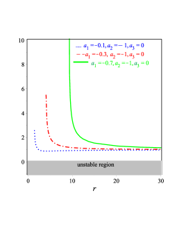
(a)  Stability of the black hole for the case $a_{3}=0$

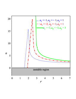
(b)  Stability of the black hole for the case $a_{3}\neq 0$

Figure 1: Schematic plot of Eq. (46), namely $\sigma^{2}$ versus the coordinate $r$ using the two black holes (III.1) and (III.1).

IV Thermodynamics of the black hole

Here we are going to study the thermodynamical quantities of the black holes (III.1) and (III.1). The temperature of a black hole is defined as Sheykhi (2012); Hendi et al. (2010); Sheykhi et al. (2010); Wang et al. (2019)

$$T_{(1,2)}=\frac{\xi_{\pm}}{2\pi}=\frac{r_{(1,2)}-r_{(2,1)}}{4\pi r_{(1,2)}{}^{2}}\,,$$ (47)

where $r_{(1,2)}$ are the inner and outer horizons of the spacetime. The Hawking entropy of the horizons is defined as

$$\psi_{(1,2)}=\frac{1}{4}A_{(1,2)}\,f_{R}\,,$$ (48)

where $A_{(1,2)}$ is the area of the horizons. The quasi-local energy is figured out as Cognola et al. (2011); Sheykhi (2012); Hendi et al. (2010); Sheykhi et al. (2010); Zheng and Yang (2018a)

$$E\left(r_{(1,2)}\right)=\frac{1}{4}\displaystyle{\int}\left[2f_{{R}}\leavevmode\nobreak\ r_{(1,2)}+r_{(1,2)}{}^{2}\left\{f(R(r_{(1,2)}))-R(r_{(1,2)})f_{R}\leavevmode\nobreak\ r_{(1,2)}\right\}\right]dr_{(1,2)}\,.$$ (49)

Finally, the Gibbs free energy in the grand canonical ensemble, is figured out as Kim and Kim (2012)

$$G(r_{(1,2)})=E(r_{(1,2)})-T(r_{(1,2)})S(r_{(1,2)})\,.$$ (50)

The black hole (III.1) is characterized by the mass $M$ and the parameter $a_{1}$ and when the parameter $a_{1}$ is vanishing we get the Schwarzschild black hole which corresponds to GR. To find the horizons of the black hole, (III.1), we put $\mu(r)=0$ and get four lengthy real positive roots. The metric potentials of the black hole (III.1) are drawn in Fig. 2 1(a). From Fig. 2 1(a), we can easy see the two positive horizons of the metric potentials $\mu(r)$. It is easy to check that the degenerate horizon for the metric potential $\mu(r)$ is happened for a specific values of $(a_{1},M,r)\equiv(-0.043,0.5,0.5)$, respectively, which correspond to the Nariai black hole. The degenerate behavior is shown in Fig. 2 1(b). Fig. 2 1(b) shows that the horizon $r_{1}$ increases as $a_{1}$ increases while $r_{2}$ decreases as $a_{1}$ decreases. As we observe from Fig. 2 1(b) that as $a_{1}$ increases and $M$ decrease i,e, $a_{1}>M$, we enter in a parameter region where there is no horizon, and thus the central singularity is a naked singularity.

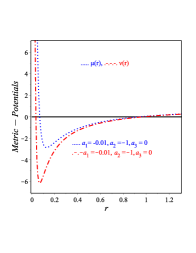
(a)  The metric potentials of the black hole (III.1)

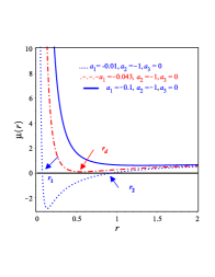
(b)  The horizons of the black hole (III.1) of the metric potential $\mu$

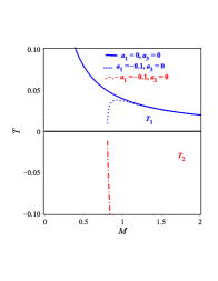
(c)  Hawking temperature of the black hole (III.1)

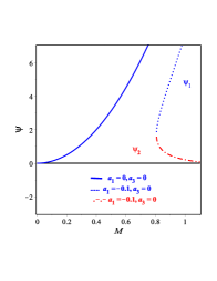
(d)  The entropy of the black hole (III.1)

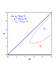
(e)  The quasi-local energy of the black hole (III.1)

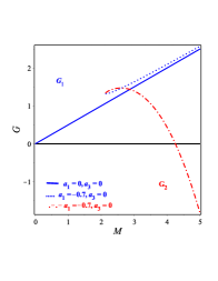
(f)  The free energy of the black hole (III.1)

Figure 2: Schematic plots of thermodynamical quantities of the black hole solution (III.1): 1(a) shows the behavior of the metric potentials $\mu$ and $\nu$; 1(b) Typical behaviour of the horizons of the metric potential $\mu(r)$ given by (III.1) ; 1(c) typical behaviour of the horizon temperature, (51), which shows that $T_{1}$ has a positive decreasing value while $T_{2}$ has a negative increasing value; 1(d) typical behaviour of the horizon entropy, (52), which shows that $\psi_{(1,2)}$ always has positive values, $\psi_{1}$ increases with $M$ wile $\psi_{2}$ has positive decreasing value; 1(e) typical behaviour of the quasi-local energy, (53), that indicates that $E_{(1,2)}$ has positive increasing values and also $E_{1}>E_{2}$; 1(f) typical behaviour of the horizon Gibbs free energy which shows that $G_{1}$ is positive while $G_{2}$ starts with positive value and as $M$ increase it becomes negative.

Using Eq. (47), we get the Hawking temperature in the form

$$T_{(1,2)}=\pm\frac{\sqrt{4M^{2}+26a_{1}}}{\pi\left(2M\pm\sqrt{4M^{2}+26a_{1}}\right)^{2}}\,.$$ (51)

The behavior of the Hawking temperature given by Eq. (51) is drawn in Fig. 2 1(c) which shows that $T_{1}>T_{2}$. As Fig. 2 1(c) shows that the $T_{1}$ has a decreasing positive temperature while $T_{2}$ has an increasing negative temperature.

Using Eq. (48) we get the entropy of black hole (III.1) in the form

$$\psi_{(1,2)}=\frac{\pi\left(4M^{2}\pm 2M\sqrt{4M^{2}+26a_{1}}+15a_{1}\right)}{2}\,.$$ (52)

The behavior of the entropy is given in Fig. 1 1(d) which shows an increasing value for $\psi_{1}$ and decreasing value for $\psi_{2}$. Using Eq. (49) we calculate the quasi-local energy and get

$$E_{(1,2)}=\frac{\pm 6M\left(4M^{2}-3a_{1}\right)\sqrt{4M^{2}+26a_{1}}+96M^{4}+588a_{1}M^{2}\pm 6M\left(4M^{2}+26a_{1}\right)^{3/2}+398a_{1}{}^{2}}{3\left(2M\pm\sqrt{4M^{2}+26a_{1}}\right)^{3}}\,.$$ (53)

The behavior of the quasi-local energies are shown in Fig. 1 1(e) which also shows positive increasing values for $E_{(1,2)}$ and also shows $E_{1}>E_{2}$. Finally, we use Eqs. (51), (52) and (53) in Eq. (50) to calculate the Gibbs free energies. The behavior of these free energies are shown in Fig. 1 1(f) which shows positive increasing value for $G_{1}$ and $G_{2}$ start with positive decreasing value then it becomes negative value.

IV.1 Thermodynamics of the black hole (III.1) that has asymptote flat AdS/dS

In this subsection, we are going to study the black hole (III.1) which is characterized by the mass of the black hole $M$, the parameter $a_{1}$ and a positive cosmological effective constant. The metric potentials of the black hole (6) are drawn in Fig. 3 1(a). From Fig. 3 1(a), we can easily see the two horizons of the metric potentials $\mu(r)$ and $\nu(r)$. To find the horizons of this black hole, (6), we put $\mu(r)=0$ in Eq. (6). This gives four roots two of them are real and the others are imaginary. These real roots are lengthy however, their behaviors are drawn in Fig. 3 2(b). It is easy to check that the degenerate horizon for the metric potential $\mu(r)$ given by Eq. (6) is happened for a specific values for $\left(a_{1},M,r,\Lambda_{\mathrm{eff}}\right)\equiv(-0.035,0.5,0.3881986644,1)$, respectively which corresponds to the Nariai black hole. The degenerate behavior is shown is Fig. 3 2(b) which shows that the horizon $r_{1}$ increases with $a_{1}$ while $r_{2}$ decreases.

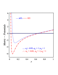
(a)  The metric potential of black hole (III.1)

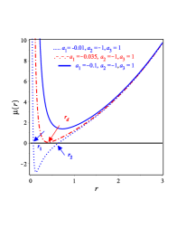
(b)  The horizons of the black hole (III.1) of the metric potential $\mu$

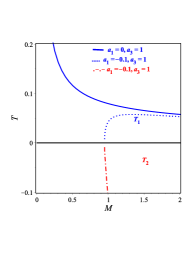
(c)  Hawking temperature of black hole (III.1)

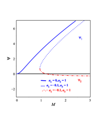
(d)  The entropy of the black hole (III.1)

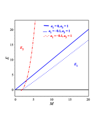
(e)  The quasi-local energy of the black hole (III.1)

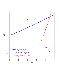
(f)  The free energy of the black hole (III.1)

Figure 3: Schematic plots of thermodynamical quantities of the black hole solution (III.1): 1(a) shows the behavior of the metric potentials $\mu$ and $\nu$; 1(b) Typical behaviour of the horizons of the metric potential $\mu(r)$ given by (III.1); 1(c) typical behaviour of the horizon temperature which shows that $T_{1}$ has a positive decreasing value while $T_{2}$ has a negative increasing value; 1(d) typical behaviour of the horizon entropy which shows that $\psi_{1}$ has an increasing value as $M$ increases while $\psi_{2}$ is positive then becomes negative as $M$ increases; 1(e) typical behaviour of the quasi-local energy that indicates that $E_{(1,2)}$ has positive increasing values and also $E_{2}>E_{1}$; 1(f) typical behaviour of the horizon Gibbs free energy which shows that $G_{1}$ is negative while $G_{2}$ starts with negative value and as $M$ increase it becomes positive.

Using Eq. (47) we draw the behavior of the Hawking temperatures in Fig. 3 1(c) which shows that $T_{1}>T_{2}$. As Fig. 3 1(c) shows that the $T_{1}$ has decreasing positive temperature while $T_{2}$ has increasing negative temperature.

Using Eq. (48), we draw the entropy in Fig. 3 2(d) which shows increasing value for $\psi_{1}$ and decreasing value for $\psi_{2}$. Using Eq. (49) we calculate the quasi-local energy that is drawn in Fig. 3 2(e) which also shows positive increasing value for $E_{(1,2)}$. Finally, we use Eqs. (51), (52) and (53) in Eq. (50) to calculate the Gibbs free energies. The behavior of these free energies are shown in Fig. 3 2(f) which shows negative increasing value for $G_{1}$ while $G_{2}$ starts with negative value and as $M$ increases it becomes positive.

By the same procedure we can study the case dS, i.e., $\Lambda_{\mathrm{eff}}a_{3}<0$ and show the behaviour of their thermodynamical physical quantities.

IV.2 First law of thermodynamics of the BHs (III.1) and (III.1)

It is important for any black hole to check its validity of the first law of thermodynamics. Therefore, we will use the formula of this law in the frame of $f(R)$ as Zheng and Yang (2018b)

$$dE=Td\psi-PdV\,,$$ (55)

with $E$, $\psi$, $T$, $P$, and $V$ are the quasi-local energy, the Hawking entropy, the Hawking temperature and the radial component of the stress-energy tensor that serves as a thermodynamic pressure, $P=T_{r}{}^{r}\mid_{\pm}$, and the geometric volume respectively. The pressure, in the context of $f(R)$ gravitational theory, is figured as Zheng and Yang (2018b)

$$P=-\frac{1}{8\pi}\left\{\frac{{F}_{1}}{r_{\pm}{}^{2}}+\frac{1}{2}(f({R})-{R}{F}_{1})\right\}+\frac{1}{4}\left(\frac{2{F}_{1}}{r_{\pm}}+{F}^{\prime}_{1}\right)T\,.$$ (56)

For the flat spacetime (III.1) if we neglect $O\left(\frac{1}{r^{3}}\right)$ and $O\left(\frac{1}{r^{4}}\right)$ to make the calculations more applicable, we get

$$r_{{}_{(1,2)}}=\frac{2M\pm\sqrt{4M^{2}+26a_{1}}}{2}\,,\qquad\psi_{{}_{(1,2)}}=\frac{\pi\left(4M^{2}\pm 2\sqrt{4M^{2}+26a_{1}}+15a_{1}\right)}{2}\,,\qquad T_{{}_{(1,2)}}=\pm\frac{\sqrt{4M^{2}+26a_{1}}}{\pi\,\left(2M\pm\sqrt{4M^{2}+26a_{1}}\right)^{2}}\,,$$

$$E_{{}_{(1,2)}}=\frac{2\left(\pm 6M\sqrt{4M^{2}+26a_{1}}\left[8M^{2}+23a_{1}\right]+48M^{4}+294a_{1}M^{2}+199a_{1}{}^{2}\right)}{3\left(2M\pm\sqrt{4M^{2}+26a_{1}}\right)^{3}}\,,$$

$$P_{{}_{(1,2)}}=\frac{4a_{1}\left(10M\sqrt{4M^{2}+26a_{1}}+20M^{2}+69a_{1}\right)}{\left(2M\pm\sqrt{4M^{2}+26a_{1}}\right)^{4}}\,.$$ (57)

Using (IV.2) in (56), we can prove that the first law of the flat spacetime is verified. Repeating the same procedure for the AdS/dS, we get

$$r_{{}_{(1,2)}}=\frac{2M\pm\sqrt{4M^{2}+26a_{1}}}{2}\,,\qquad\psi_{{}_{(1,2)}}=\frac{\pi\left(4M^{2}\pm 2\sqrt{4M^{2}+26a_{1}}+15a_{1}\right)}{2}\,,\qquad T_{{}_{(1,2)}}=\pm\frac{\sqrt{4M^{2}+26a_{1}}}{\pi\,\left(2M\pm\sqrt{4M^{2}+26a_{1}}\right)^{2}}\,,$$

$$E_{{}_{(1,2)}}=\frac{2\left(\pm 6M\sqrt{4M^{2}+26a_{1}}\left[8M^{2}+23a_{1}\right]+48M^{4}+294a_{1}M^{2}+199a_{1}{}^{2}\right)}{3\left(2M\pm\sqrt{4M^{2}+26a_{1}}\right)^{3}}\,,$$

$$P_{{}_{(1,2)}}=\frac{4a_{1}\left(10M\sqrt{4M^{2}+26a_{1}}+20M^{2}+69a_{1}\right)}{\left(2M\pm\sqrt{4M^{2}+26a_{1}}\right)^{4}}\,.$$ (58)

Substituting the form of $r$ into the thermodynamical quantities we get

$$dE=\frac{4m^{4}+b^{2}m^{2}+b^{4}}{8\,m^{4}}\,,\qquad\psi=\frac{\pi\left(40m^{4}-20m^{2}b^{2}-8mb^{4}-25b^{4}\right)}{10\,m^{3}}\,,\qquad T=\frac{4mb^{4}-20m^{4}+35b^{4}+15m^{2}b^{2}}{160\,\pi\,m^{5}}\,,$$

$$P=-\frac{b^{2}\left(30m^{2}+75b^{2}+8mb^{2}\right)}{640\,\pi\,m^{6}}\,.$$ (59)

If we use Eq. (IV.2) in (56), we can verify the first law of thermodynamics for the BH (III.1).

If one repeats the same procedure for the BH (III.1), one can verify the first law of thermodynamics provided that we neglect all the quantities containing $b$ to make the calculation easier to carry out.

V Discussion and conclusions

It is well-known that spherically symmetric spacetime is an essential spacetime in GR for many reasons: First because it is the easiest geometry that one can start to use in the study of GR. In this exposition, we tackle the problem of applying the charged field equations of $f(R)$ to a spherically symmetric spacetime with two unknown functions. We derive a highly nonlinear five differential equations in four unknowns, two of the metric potential, the third is the derivative of $f(R)$, and the fourth is the gauge potential of the Maxwell field. We study some limits of this system of differential equations to test its compatibility with the previous studies and got consistent results of BHs derived for constant and non-constant Ricci scalar. Then we turn our attention to the general case and solve this system by assuming a specific form of the derivative of $f(R)$. This assumption involves one constant that when it equals zero we got the GR theory limit. We derive the form of the metric potential and the gauge potential of the Maxwell field and show they depend on the convolution and error functions respectively. Under some constraints, if these functions are set zero, we got to the Schwarzschild BH of GR which means that in the limit of higher-order curvature theory, we cannot generate the Reissner-Nordström BH. This gives us an indication that the effect of the higher-order curvature terms restored in the convolution and error functions.

To gain some physics of these BHs we studied their asymptotes and show that we have a constant of integration that plays an important role in the asymptote, i.e., when this constant is vanishing/non-vanishing, we got two different asymptotes of the BHs, a flat and AdS/dS spacetimes respectively. Moreover, we studied the invariants of these BHs and showed that their singularities are milder than those of GR BH. By the use of the geodesic deviation, we derived the conditions of stability of those BHs and showed their stable areas as shown in Figs. 1 0(a) and 0(b). Also, we have calculated some thermodynamics quantities like the Hawking temperature, entropy, quasi-local energy, and the Gibbs free energy to know the behavior of those BHs analytic and graphically and show in detail that such BHs satisfy the first law of thermodynamics. Finally, if we use the results of odd perturbation presented in Elizalde et al. (2020), we can show easily that the BHs derived in this study are stable.

To conclude, we have derived new charged BHs in the context of $f(R)$ that their Ricci scalars are not constant. The originality of those BHs comes from the constant that involves the assumption of the derivative function of $f(R)$. If we follow the same procedure but with another assumption of the derivative function of $f(R)$, we can get new BHs but this needs more study because of the complication of the system. This will be done elsewhere.

Appendix A

The form of Kretschmann scalar

The exact form of the Kretschmann scalar is given as:

$$R_{\mu\nu\rho\sigma}R^{\mu\nu\rho\sigma}=\frac{1}{\left({r}^{2}+a_{1}\right)^{2}{r}^{10}}\Bigg{\{}16\mathrm{e}^{{\frac{3a_{1}}{{r}^{2}}}}\Bigg{[}3\left(3{a_{1}}^{4}+12\,{a_{1}}^{2}{r}^{4}+6\,{a_{1}}^{3}{r}^{2}-2a_{1}{r}^{6}+{r}^{8}\right){H}^{2}-4{H}_{2}\left({r}^{2}a_{1}+{r}^{4}+6{a_{1}}^{2}\right){r}^{2}a_{1}H+4\times$$

$$H_{2}{}^{2}{a_{1}}^{2}\left(2{a_{1}}^{2}+2{r}^{2}a_{1}+{r}^{4}\right)\Bigg{]}\left(\int\!\frac{{H}_{1}{\mathrm{e}^{-{\frac{3a_{1}}{2{r}^{2}}}}}\left({r}^{2}+13a_{1}\right){r}^{2}}{\left({r}^{2}+a_{1}\right)\left(2a_{1}[{H}_{1}{H}_{2}-{H}{H}_{3}]-3{H}_{1}{H}{r}^{2}\right)}{dr}\right)^{2}-16\Bigg{[}\Bigg{\{}\Bigg{(}18\left(2{a_{1}}^{2}{r}^{2}+2{r}^{4}a_{1}-{r}^{6}+{a_{1}}^{3}\right){H}_{1}$$

$$-2\left({r}^{2}a_{1}+{r}^{4}+18{a_{1}}^{2}\right){r}^{2}H_{3}\Bigg{)}{H}+2{H}_{2}\left(\left(2{r}^{6}+5{r}^{4}a_{1}\right){H}_{1}+2a_{1}{H}_{3}\left(2{a_{1}}^{2}+2{r}^{2}a_{1}+{r}^{4}\right)\right)\Bigg{\}}{r}^{3}a_{1}{\mathrm{e}^{{\frac{3}{a_{1}}{2{r}^{2}}}}}$$

$$\times\int\!\frac{{\mathrm{e}^{-{\frac{3a_{1}}{2{r}^{2}}}}}{H}\left({r}^{2}+13\,a_{1}\right)}{{r}\left({r}^{2}+a_{1}\right)\left(2a_{1}[{H}_{1}{H}_{2}-{H}{H}_{3}]-3\,{H}_{1}{H}{r}^{2}\right)}{dr}+3\left(3{a_{1}}^{4}+12{a_{1}}^{2}{r}^{4}+6{a_{1}}^{3}{r}^{2}-2a_{1}{r}^{6}+{r}^{8}\right)a_{2}{\mathrm{e}^{{\frac{3a_{1}}{2{r}^{2}}}}}{H}{}^{2}$$

$$+\Bigg{\{}9a_{1}ra_{3}\,{\mathrm{e}^{{\frac{3a_{1}}{2{r}^{2}}}}}\left(2\,{a_{1}}^{2}{r}^{2}+2\,{r}^{4}a_{1}-{r}^{6}+{a_{1}}^{3}\right){H}_{1}-2\left({r}^{2}a_{1}+{r}^{4}+18{a_{1}}^{2}\right){r}^{3}a_{1}{\mathrm{e}^{{\frac{3a_{1}}{2{r}^{2}}}}}a_{3}\,{H}_{3}-4\left({r}^{2}a_{1}+{r}^{4}+18{a_{1}}^{2}\right)a_{2}\,a_{1}{\mathrm{e}^{{\frac{3a_{1}}{2{r}^{2}}}}}{H}_{2}$$

$$+{r}^{3}\left({\mathrm{e}^{-3/2\,{\frac{a_{1}}{{r}^{2}}}}}\left(5a_{1}-{r}^{2}\right)\left({r}^{2}+13a_{1}\right){\mathrm{e}^{{\frac{3a_{1}}{2{r}^{2}}}}}-\left({r}^{2}+a_{1}\right)^{2}\right)\Bigg{\}}{r}^{2}{H}+2{H}_{2}\Bigg{[}\left(5a_{1}+2{r}^{2}\right){r}^{7}a_{3}\,{H}_{1}+\Bigg{\{}2{r}^{3}a_{3}\left(2{a_{1}}^{2}+2{r}^{2}a_{1}+{r}^{4}\right){H}_{3}$$

$$+a_{2}\,\left(2{a_{1}}^{2}+2{r}^{2}a_{1}+{r}^{4}\right){H}_{2}-{\mathrm{e}^{-3/2\,{\frac{a_{1}}{{r}^{2}}}}}{r}^{3}\left({r}^{2}+13a_{1}\right)\Bigg{\}}a_{1}\Bigg{]}a_{1}{\mathrm{e}^{{\frac{3a_{1}}{2{r}^{2}}}}}\Bigg{]}{\mathrm{e}^{{\frac{3}{a_{1}}{2{r}^{2}}}}}\int\!\frac{{H}_{1}{\mathrm{e}^{-{\frac{3a_{1}}{2{r}^{2}}}}}\left({r}^{2}+13\,a_{1}\right){r}^{2}}{\left({r}^{2}+a_{1}\right)\left(2\,{H}_{1}a_{1}{H}_{2}-3\,{H}{H}_{1}{r}^{2}-2\,{H}a_{1}{H}_{3}\right)}{dr}$$

$$+16\left(3\left(2{r}^{8}+6\,{a_{1}}^{3}{r}^{2}+3{a_{1}}^{4}+6\,{a_{1}}^{2}{r}^{4}+2/3\,a_{1}{r}^{6}\right)H_{1}{}^{2}+4\left(5a_{1}+2{r}^{2}\right){r}^{4}a_{1}H_{3}H_{1}+4{a_{1}}^{2}{H}_{3}{}^{2}\left(2{a_{1}}^{2}+2{r}^{2}a_{1}+{r}^{4}\right)\right){r}^{6}{\mathrm{e}^{{\frac{3a_{1}}{{r}^{2}}}}}$$

$$\times\left(\int\!\frac{\frac{\mathrm{e}^{{\frac{3a_{1}}{2{r}^{2}}}}}{H}\left({r}^{2}+13\,a_{1}\right)}{r\left({r}^{2}+a_{1}\right)\left(2a_{1}[H_{1}H_{2}-HH_{3}]-3\,{H}_{1}H{r}^{2}\right)}{dr}\right)^{2}+16{r}^{3}{\mathrm{e}^{{\frac{3a_{1}}{2{r}^{2}}}}}\Bigg{\{}a_{2}\,\Bigg{[}9\left(2\,{a_{1}}^{2}{r}^{2}+2\,{r}^{4}a_{1}-{r}^{6}+{a_{1}}^{3}\right)H_{1}-2{r}^{2}H_{3}\Bigg{\{}{r}^{2}a_{1}$$

$$+{r}^{4}+18{a_{1}}^{2}\Bigg{\}}\Bigg{]}a_{1}{\mathrm{e}^{{\frac{3a_{1}}{2{r}^{2}}}}}H+3{r}^{3}\left(2{r}^{8}+2{a_{1}}^{3}{r}^{2}+{a_{1}}^{4}+6{a_{1}}^{2}{r}^{4}+2a_{1}{r}^{6}\right){\mathrm{e}^{{\frac{3a_{1}}{2{r}^{2}}}}}a_{3}H_{1}{}^{2}+{r}^{4}\Bigg{\{}2\left(5a_{1}+2{r}^{2}\right)a_{1}{\mathrm{e}^{{\frac{3a_{1}}{{2r}^{2}}}}}[2a_{3}H_{3}r^{3}+a_{2}H_{2}]$$

$$\left({\mathrm{e}^{-{\frac{3a_{1}}{2{r}^{2}}}}}\left(2a_{1}-{r}^{2}\right)\left({r}^{2}+13a_{1}\right){\mathrm{e}^{3/2\,{\frac{a_{1}}{{r}^{2}}}}}-\left({r}^{2}+a_{1}\right)^{2}\right)r\Bigg{\}}H_{1}+\Bigg{\{}4{r}^{3}a_{3}\,\left(2{a_{1}}^{2}+2{r}^{2}a_{1}+{r}^{4}\right){H}_{3}+4a_{2}\,\left(2{a_{1}}^{2}+2{r}^{2}a_{1}+{r}^{4}\right){H}_{2}$$

$$-{\mathrm{e}^{-{\frac{3a_{1}}{2{r}^{2}}}}}{r}^{3}\left({r}^{2}+13a_{1}\right)\Bigg{\}}{a_{1}}^{2}{\mathrm{e}^{{\frac{3a_{1}}{2{r}^{2}}}}}H_{3}\Bigg{\}}\int\!\frac{{\mathrm{e}^{-{\frac{3a_{1}}{2{r}^{2}}}}}H\left({r}^{2}+13\,a_{1}\right)}{{r}\left({r}^{2}+a_{1}\right)\left(2\,H_{1}a_{1}{H}_{2}-3\,HH_{1}{r}^{2}-2\,Ha_{1}H_{3}\right)}{dr}$$

$$+12\left(3{a_{1}}^{4}+6{a_{1}}^{2}{r}^{4}+6\,{a_{1}}^{3}{r}^{2}-2a_{1}{r}^{6}+{r}^{8}\right){a_{2}}^{2}{\mathrm{e}^{{\frac{3a_{1}}{{r}^{2}}}}}H^{2}+8a_{2}\,{r}^{2}\Bigg{\{}9a_{1}ra_{3}\,{\mathrm{e}^{{\frac{3a_{1}}{2{r}^{2}}}}}\left(2\,{a_{1}}^{2}{r}^{2}+2\,{r}^{4}a_{1}-{r}^{6}+{a_{1}}^{3}\right)H_{1}-2\Bigg{[}{r}^{2}a_{1}+{r}^{4}$$

$$+18{a_{1}}^{2}\Bigg{]}{r}^{3}a_{1}{\mathrm{e}^{{\frac{3a_{1}}{2{r}^{2}}}}}a_{3}\,H_{3}-2\left({r}^{2}a_{1}+{r}^{4}+18{a_{1}}^{2}\right)a_{2}\,a_{1}{\mathrm{e}^{{\frac{3a_{1}}{2{r}^{2}}}}}H_{2}+\,{r}^{3}\Bigg{[}{\mathrm{e}^{-{\frac{3a_{1}}{2{r}^{2}}}}}\left(5a_{1}-{r}^{2}\right)\left({r}^{2}+13a_{1}\right){\mathrm{e}^{{\frac{3a_{1}}{2{r}^{2}}}}}-\left({r}^{2}+a_{1}\right)^{2}\Bigg{]}\Bigg{\}}{\mathrm{e}^{{\frac{3a_{1}}{2{r}^{2}}}}}H$$

$$+12{r}^{6}\left(2{r}^{8}+6\,{a_{1}}^{3}{r}^{2}+3{a_{1}}^{4}+6\,{a_{1}}^{2}{r}^{4}+a_{1}{r}^{6}\right){\mathrm{e}^{{\frac{3a_{1}}{{r}^{2}}}}}{a_{3}}^{2}H_{1}{}^{2}+8{r}^{7}{\mathrm{e}^{{\frac{3a_{1}}{2{r}^{2}}}}}\Bigg{[}2\left(5a_{1}+{r}^{2}\right){r}^{3}a_{1}{\mathrm{e}^{{\frac{3a_{1}}{2{r}^{2}}}}}[r^{3}a_{3}\,H_{3}+a_{2}H_{2}]$$

$$+\left({\mathrm{e}^{-{\frac{3a_{1}}{2{r}^{2}}}}}\left(2a_{1}-{r}^{2}\right)\left({r}^{2}+13a_{1}\right){\mathrm{e}^{{\frac{3a_{1}}{2{r}^{2}}}}}-\left({r}^{2}+a_{1}\right)^{2}\right)r\Bigg{]}a_{3}\,H_{1}+16{r}^{6}{a_{1}}^{2}{\mathrm{e}^{{\frac{3a_{1}}{{r}^{2}}}}}{a_{3}}^{2}\left(2{a_{1}}^{2}+2{r}^{2}a_{1}+{r}^{4}\right)\left(H_{3}\right)^{2}$$

$$+16\left(2a_{2}\,\left(2{a_{1}}^{2}+2{r}^{2}a_{1}+{r}^{4}\right)H_{2}-{\mathrm{e}^{-{\frac{13a_{1}}{2{r}^{2}}}}}{r}^{3}\left({r}^{2}+13a_{1}\right)\right){r}^{3}{a_{1}}^{2}{\mathrm{e}^{{\frac{3a_{1}}{{r}^{2}}}}}a_{3}\,H_{3}+16\,{a_{2}}^{2}{a_{1}}^{2}{\mathrm{e}^{{\frac{3a_{1}}{2{r}^{2}}}}}\left(2{a_{1}}^{2}+2{r}^{2}a_{1}+{r}^{4}\right)H_{2}{}^{2}$$

$$-16{\mathrm{e}^{-3/2\,{\frac{a_{1}}{{r}^{2}}}}}a_{2}\,{r}^{3}{a_{1}}^{2}{\mathrm{e}^{{\frac{3a_{1}}{{r}^{2}}}}}\left({r}^{2}+13a_{1}\right)H_{2}+4\left({\mathrm{e}^{-{\frac{3a_{1}}{{r}^{2}}}}}\left({r}^{2}+13a_{1}\right)^{2}{\mathrm{e}^{{3\frac{a_{1}}{{r}^{2}}}}}+\left({r}^{2}+a_{1}\right)^{2}\right){r}^{6}\Bigg{\}}\,.$$

The above equation shows that the Kretschmann scalar has a true singularity at the origin. By the same method one can show that the squared of the Ricci tensor and the Ricci scalar have a singularity at the origin.

References

- Akiyama et al. (2019a) K. Akiyama et al. (Event Horizon Telescope), Astrophys. J. 875, L1 (2019a), arXiv:1906.11238 [astro-ph.GA] .
- Akiyama et al. (2019b) K. Akiyama et al. (Event Horizon Telescope), Astrophys. J. Lett. 875, L6 (2019b), arXiv:1906.11243 [astro-ph.GA] .
- Ayzenberg and Yunes (2018) D. Ayzenberg and N. Yunes, Class. Quant. Grav. 35, 235002 (2018), arXiv:1807.08422 [gr-qc] .
- Will (2005) C. M. Will, Annalen Phys. 15, 19 (2005), arXiv:gr-qc/0504086 .
- Will (2006) C. M. Will, Living Rev. Rel. 9, 3 (2006), arXiv:gr-qc/0510072 .
- Yunes and Siemens (2013) N. Yunes and X. Siemens, Living Rev. Rel. 16, 9 (2013), arXiv:1304.3473 [gr-qc] .
- Milgrom (1983) M. Milgrom, Astrophys. J. 270, 371 (1983).
- Bekenstein and Milgrom (1984) J. Bekenstein and M. Milgrom, Astrophys. J. 286, 7 (1984).
- Milgrom and Sanders (2003) M. Milgrom and R. H. Sanders, Astrophys. J. Lett. 599, L25 (2003), arXiv:astro-ph/0309617 .
- Perlmutter et al. (1999) S. Perlmutter et al. (Supernova Cosmology Project), Astrophys. J. 517, 565 (1999), arXiv:astro-ph/9812133 .
- Riess et al. (1998) A. G. Riess et al. (Supernova Search Team), Astron. J. 116, 1009 (1998), arXiv:astro-ph/9805201 [astro-ph] .
- Penrose (1965) R. Penrose, Phys. Rev. Lett. 14, 57 (1965).
- Hawking (1976) S. W. Hawking, Phys. Rev. D 14, 2460 (1976).
- Christodoulou (1991) D. Christodoulou, Commun. Pure Appl. Math. 44, 339 (1991).
- Rovelli (1996) C. Rovelli, Phys. Rev. Lett. 77, 3288 (1996).
- Ashtekar et al. (2006) A. Ashtekar, T. Pawlowski, and P. Singh, Phys. Rev. Lett. 96, 141301 (2006), arXiv:gr-qc/0602086 .
- Nojiri and Odintsov (2011) S. Nojiri and S. D. Odintsov, Phys. Rept. 505, 59 (2011), arXiv:1011.0544 [gr-qc] .
- Capozziello et al. (2006) S. Capozziello, S. Nojiri, S. D. Odintsov, and A. Troisi, Phys. Lett. , 135 (2006), arXiv:astro-ph/0604431 [astro-ph] .
- Lanczos (1932) C. Lanczos, Phys. Rev. 39, 716 (1932).
- Lanczos (1938) C. Lanczos, Annals Math. 39, 842 (1938).
- Lovelock (1971) D. Lovelock, J. Math. Phys. 12, 498 (1971).
- Padmanabhan and Kothawala (2013) T. Padmanabhan and D. Kothawala, Phys. Rept. 531, 115 (2013), arXiv:1302.2151 [gr-qc] .
- Dadhich et al. (2016) N. Dadhich, R. Durka, N. Merino, and O. Miskovic, Phys. Rev. D 93, 064009 (2016), arXiv:1511.02541 [hep-th] .
- Shiromizu et al. (2000) T. Shiromizu, K.-i. Maeda, and M. Sasaki, Phys. Rev. D 62, 024012 (2000), arXiv:gr-qc/9910076 .
- Awad and Nashed (2017) A. Awad and G. Nashed, Journal of Cosmology and Astroparticle Physics 2017 (2017), 10.1088/1475-7516/2017/02/046.
- Harko and Mak (2004) T. Harko and M. Mak, Phys. Rev. D 69, 064020 (2004), arXiv:gr-qc/0401049 .
- Carames et al. (2013) T. Carames, M. Guimaraes, and J. Hoff da Silva, Phys. Rev. D 87, 106011 (2013), arXiv:1205.4980 [gr-qc] .
- Haghani et al. (2012) Z. Haghani, H. R. Sepangi, and S. Shahidi, JCAP 02, 031 (2012), arXiv:1201.6448 [gr-qc] .
- Chakraborty and SenGupta (2015) S. Chakraborty and S. SenGupta, Eur. Phys. J. C 75, 11 (2015), arXiv:1409.4115 [gr-qc] .
- Brans and Dicke (1961) C. Brans and R. H. Dicke, Phys. Rev. 124, 925 (1961).
- Horndeski (1974) G. W. Horndeski, Int. J. Theor. Phys. 10, 363 (1974).
- Sotiriou and Zhou (2014) T. P. Sotiriou and S.-Y. Zhou, Phys. Rev. Lett. 112, 251102 (2014), arXiv:1312.3622 [gr-qc] .
- Babichev et al. (2016) E. Babichev, C. Charmousis, and A. Lehébel, Class. Quant. Grav. 33, 154002 (2016), arXiv:1604.06402 [gr-qc] .
- Riess et al. (2004) A. G. Riess et al. (Supernova Search Team), Astrophys. J. 607, 665 (2004), arXiv:astro-ph/0402512 [astro-ph] .
- Cognola et al. (2005) G. Cognola, E. Elizalde, S. Nojiri, S. D. Odintsov, and S. Zerbini, JCAP 02, 010 (2005), arXiv:hep-th/0501096 .
- Cooney et al. (2010) A. Cooney, S. DeDeo, and D. Psaltis, Phys. Rev. D 82, 064033 (2010).
- Guo and Frolov (2013) J.-Q. Guo and A. V. Frolov, Phys. Rev. D 88, 124036 (2013).
- Sotiriou and Faraoni (2010) T. P. Sotiriou and V. Faraoni, Rev. Mod. Phys. 82, 451 (2010).
- Hendi (2010) S. Hendi, Phys. Lett. B 690, 220 (2010), arXiv:0907.2520 [gr-qc] .
- Capozziello and De Laurentis (2011) S. Capozziello and M. De Laurentis, Phys. Rept. 509, 167 (2011), arXiv:1108.6266 [gr-qc] .
- Maeda (1989) K.-i. Maeda, Phys. Rev. D 39, 3159 (1989).
- Antoniadis et al. (2020) I. Antoniadis, A. Lykkas, and K. Tamvakis, JCAP 04, 033 (2020), arXiv:2002.12681 [gr-qc] .
- Amendola et al. (2007) L. Amendola, R. Gannouji, D. Polarski, and S. Tsujikawa, Phys. Rev. D 75, 083504 (2007).
- Li and Barrow (2009) B. Li and J. D. Barrow, Phys. Rev. D 79, 103521 (2009).
- Hu and Sawicki (2007) W. Hu and I. Sawicki, Phys. Rev. D 76, 104043 (2007).
- Starobinsky (2007) A. A. Starobinsky, JETP Lett. 86, 157 (2007), arXiv:0706.2041 [astro-ph] .
- Capozziello et al. (2016) S. Capozziello, S. J. Gionti, Gabriele, and D. Vernieri, JCAP 1601, 015 (2016), arXiv:1508.00441 [gr-qc] .
- Multamäki and Vilja (2006) T. Multamäki and I. Vilja, Phys. Rev. D 74, 064022 (2006).
- Nashed (2018a) G. G. L. Nashed, European Physical Journal Plus 133, 18 (2018a).
- Nashed (2018b) G. G. L. Nashed, International Journal of Modern Physics D 27, 1850074 (2018b).
- Nashed (2002) G. Nashed, Nuovo Cimento della Societa Italiana di Fisica B 117, 521 (2002), cited By 25.
- Nashed (2018) G. G. L. Nashed, Adv. High Energy Phys. 2018, 7323574 (2018).
- Elizalde et al. (2020) E. Elizalde, G. G. L. Nashed, S. Nojiri, and S. D. Odintsov, Eur. Phys. J. C80, 109 (2020), arXiv:2001.11357 [gr-qc] .
- Nashed et al. (2019) G. G. L. Nashed, W. El Hanafy, S. D. Odintsov, and V. K. Oikonomou, (2019), arXiv:1912.03897 [gr-qc] .
- Nashed and Capozziello (2019) G. G. L. Nashed and S. Capozziello, Phys. Rev. D99, 104018 (2019), arXiv:1902.06783 [gr-qc] .
- Sultana and Kazanas (2018) J. Sultana and D. Kazanas, Gen. Rel. Grav. 50, 137 (2018), arXiv:1810.02915 [gr-qc] .
- Cañate (2018) P. Cañate, Class. Quant. Grav. 35, 025018 (2018).
- Nashed (2010) G. G. L. Nashed, Chin. Phys. B 19, 020401 (2010), arXiv:0910.5124 [gr-qc] .
- Yu et al. (2018) S. Yu, C. Gao, and M. Liu, Res. Astron. Astrophys. 18, 157 (2018), arXiv:1711.04064 [gr-qc] .
- Cañate et al. (2016) P. Cañate, L. G. Jaime, and M. Salgado, Class. Quant. Grav. 33, 155005 (2016), arXiv:1509.01664 [gr-qc] .
- Kehagias et al. (2015) A. Kehagias, C. Kounnas, D. Lüst, and A. Riotto, JHEP 05, 143 (2015), arXiv:1502.04192 [hep-th] .
- Nelson (2010) W. Nelson, Phys. Rev. D 82, 104026 (2010).
- de la Cruz-Dombriz et al. (2009) A. de la Cruz-Dombriz, A. Dobado, and A. L. Maroto, Phys. Rev. D80, 124011 (2009), [Erratum: Phys. Rev.D83,029903(2011)], arXiv:0907.3872 [gr-qc] .
- Capozziello et al. (2012) S. Capozziello, N. Frusciante, and D. Vernieri, Gen. Rel. Grav. 44, 1881 (2012), arXiv:1204.4650 [gr-qc] .
- Carroll et al. (2004) S. M. Carroll, V. Duvvuri, M. Trodden, and M. S. Turner, Phys. Rev. D70, 043528 (2004), arXiv:astro-ph/0306438 [astro-ph] .
- Buchdahl (1970) H. A. Buchdahl, mnras 150, 1 (1970).
- Nojiri and Odintsov (2003) S. Nojiri and S. D. Odintsov, Phys. Rev. , 123512 (2003), arXiv:hep-th/0307288 [hep-th] .
- Capozziello et al. (2003) S. Capozziello, V. F. Cardone, S. Carloni, and A. Troisi, Int. J. Mod. Phys. D12, 1969 (2003), arXiv:astro-ph/0307018 [astro-ph] .
- Nojiri et al. (2017) S. Nojiri, S. D. Odintsov, and V. K. Oikonomou, Phys. Rept. 692, 1 (2017), arXiv:1705.11098 [gr-qc] .
- Capozziello (2002) S. Capozziello, Int. J. Mod. Phys. D11, 483 (2002), arXiv:gr-qc/0201033 [gr-qc] .
- Capozziello et al. (2013) S. Capozziello, P. A. Gonzalez, E. N. Saridakis, and Y. Vasquez, JHEP 02, 039 (2013), arXiv:1210.1098 [hep-th] .
- Cognola et al. (2005) G. Cognola, E. Elizalde, S. Nojiri, S. D. Odintsov, and S. Zerbini, jcap 2, 010 (2005), hep-th/0501096 .
- Kalita and Mukhopadhyay (2019) S. Kalita and B. Mukhopadhyay, Eur. Phys. J. C79, 877 (2019), arXiv:1910.06564 [gr-qc] .
- Nashed (2003) G. G. L. Nashed, Chaos Solitons Fractals 15, 841 (2003), arXiv:gr-qc/0301008 [gr-qc] .
- Sheykhi (2012) A. Sheykhi, Phys. Rev. D 86, 024013 (2012).
- Hendi et al. (2010) S. H. Hendi, A. Sheykhi, and M. H. Dehghani, Eur. Phys. J. C70, 703 (2010), arXiv:1002.0202 [hep-th] .
- Sheykhi et al. (2010) A. Sheykhi, M. H. Dehghani, and S. H. Hendi, Phys. Rev. D 81, 084040 (2010).
- Wang et al. (2019) Y.-Q. Wang, Y.-X. Liu, and S.-W. Wei, Phys. Rev. D99, 064036 (2019), arXiv:1811.08795 [gr-qc] .
- Cognola et al. (2011) G. Cognola, O. Gorbunova, L. Sebastiani, and S. Zerbini, Phys. Rev. D 84, 023515 (2011).
- Zheng and Yang (2018a) Y. Zheng and R.-J. Yang, Eur. Phys. J. C78, 682 (2018a), arXiv:1806.09858 [gr-qc] .
- Kim and Kim (2012) W. Kim and Y. Kim, Phys. Lett. B718, 687 (2012), arXiv:1207.5318 [gr-qc] .
- Zheng and Yang (2018b) Y. Zheng and R. Yang, The European Physical Journal C 78 (2018b), 10.1140/epjc/s10052-018-6167-4.