Kozai Migration Naturally Explains the White Dwarf Planet WD1856b

Abstract

The Jovian-sized object WD 1856 b transits a white dwarf (WD) in a compact $1.4$-day orbit. Unlikely to have endured stellar evolution in its current orbit, WD 1856 b is thought to have migrated from much wider separations. Because the WD is old, and a member of a well-characterized hierarchical multiple, the well-known Kozai mechanism provides an effective migration channel for WD 1856 b. Moreover, the lack of tides in the star allows us to directly connect the current semi-major axis to the pre-migration one, from which we can infer the initial conditions of the system. By further demanding that successful migrators survive all previous phases of stellar evolution, we are able to constrain the mass of WD 1856 b to be $\simeq 0.7-3M_{\rm J}$ and its main sequence semi-major axis to be $\simeq 2-2.5$ au. These properties imply that WD 1856 b was born a typical gas giant. We further estimate the occurrence rate of Kozai-migrated planets around WDs to be ${\cal O}(10^{-3}{-}10^{-4})$, suggesting that WD 1856 b is the only one in the TESS sample, but implying ${\cal O}(10^{2})$ future detections by LSST. In a sense, WD 1856 b was an ordinary Jovian planet that underwent an extraordinary dynamical history.

1 Introduction

Recently, TESS observations revealed a planet-size object transiting WD 1856+534, a cool, old white dwarf (WD) with an effective temperature of $T_{\rm eff}\simeq 4700~{}$K (Vanderburg et al., 2020). WD 1856 b has an orbital period of 1.4 d and a radius of $\simeq 10R_{\oplus}$. This orbit is so compact that it is unlikely to have persisted throughout the red giant branch (RGB) and the asymptotic giant branch (AGB) phases of stellar evolution. Instead, WD 1856 b is thought to have formed at greater separations, and to have migrated inward after the main sequence (MS).

Although WD 1856 b is a cool ($<200$K) object, its orbit resembles those of the ‘hot Jupiters’ that accompany ${\sim}1\%$ of MS stars (e.g.. Howard et al., 2012). Among the proposed mechanisms of hot Jupiter migration, the von Zeipel-Lidov-Kozai (ZLK) mechanism coupled with tidal friction (Wu & Murray, 2003; Fabrycky & Tremaine, 2007) has emerged as a predictive and elegant contender, with several works suggesting that, at least in part, hot Jupiters do indeed originate from this mechanism (e.g., Naoz et al., 2012; Petrovich, 2015; Anderson et al., 2016).

Much like hot Jupiters, WD 1856 b could have migrated to its current position due to ZLK oscillations induced by a known outer companion(s) to WD 1856+534 (McCook & Sion, 1999). From Gaia astrometry, Vanderburg et al. (2020) measured the outer companion G 229-20, a double M-dwarf, to orbit WD 1856+534 at a distance of $\sim 1500$ au with an eccentricity of $\simeq 0.3$ (see Table 1). For such a wide orbit, the timescale associated to ZLK oscillations is, to quadrupole level of approximation,

$$\tau_{\rm quad}\approx 4.37\times 10^{7}\left(\frac{M_{\rm WD}}{0.5M_{\odot}}\right)^{1/2}\left(\frac{a_{\rm p,0}}{5{\rm au}}\right)^{-3/2}\text{yr}$$ (1)

which is much shorter than the cooling age of the WD, estimated to be ${\sim}6\times 10^{9}$ yr (Vanderburg et al., 2020).

Table 1: Parameters of WD 1856+534 system

WD mass ($M_{\rm WD})$	$0.518\pm 0.05\;M_{\odot}$
WD cooling age ($T_{\rm cool}$)	$5.85\pm 0.5$ Gyr
planet orbital period	$1.407$ days
planet semi-major axis ($a_{\rm p}$)	$0.0204\pm 0.0012$ au
planet radius $(R_{\rm p})$	$10.4\pm 1\;R_{\oplus}$
Mass G 229-20 A ($M_{A}$)	$0.346\pm 0.027\;M_{\odot}$
Mass G 229-20 B ($M_{B}$)	$0.331\pm 0.024\;M_{\odot}$
$M_{\rm out}=M_{A}+M_{B}$	$0.677\pm 0.051\;M_{\odot}$
A-B binary semi-major axis ($a_{\rm AB})$	$58^{+54}_{-16}$ au
outer semi-major axis ($a_{\rm out})$	$1500^{+700}_{-240}$ au
outer eccentricity $e_{\rm out}$	$0.3^{+0.19}_{-0.1}$

Despite an earlier suggestion by Agol (2011) that the ZLK mechanism could produce planets in close orbits around WDs, most theoretical efforts in this context have instead emphasized how ZLK oscillations can explain WD pollution (Hamers & Portegies Zwart, 2016; Petrovich & Muñoz, 2017; Stephan et al., 2017). In spite of this oversight, ZLK migration of gas giants around WDs is very much possible, with the requirement that the planets survive all prior stages of stellar evolution.

In this work, we exploit the distinguishing feature of ZLK migration around WDs that tidal dissipation in the host is negligible. Therefore, once the planet is parked in a circular, tidally-locked orbit, it does not decay further, in contrast to hot Jupiter systems of advanced age (e.g., Hamer & Schlaufman, 2020). By relating the current semi-major axis of WD 1856 b to the maximum attainable ZLK eccentricity, we can derive the initial separation and the planet mass that are required for WD 1856 b to have safely migrated to its current separation while avoiding tidal disruption.

2 Eccentricity Oscillations After the Main Sequence

While eccentricity oscillations take place for any initial inclination $i_{0}$ above some angle $i_{\rm crit}$ ($39.2^{\circ}$ if short-range forces are absent), actual migration is only possible at high inclinations, when the maximum eccentricity $e_{\rm max}$ surpasses a critical value $e_{\rm mig}$. Above $e_{\rm mig}$, the pericenter distance is only a few solar radii, which makes tidal dissipation effective. Likewise, when the eccentricity is above a critical value $e_{\rm dis}>e_{\rm mig}$, the separation at pericenter is so small that the planet can be tidally disrupted.

After successful migration, the semi-major axis is

$$a_{\rm p,f}\approx 2a_{\rm p,0}(1-e_{\rm max}),$$ (2a)

subject to the condition

$$e_{\rm dis}{>}e_{\rm max}{\geq}e_{\rm mig},$$ (2b)

where $a_{\rm p,0}$ is the planet’s initial semi-major axis. Equation (2a) suggests that, if $a_{\rm p,f}$ is known ($0.0204$ au in the case of WD 1856 b; Table 1), then the planet’s original orbital separation can be inferred, provided that we can calculate if $e_{\rm max}$ terms of $a_{\rm p,0}$ and other parameters of the system.

2.1 Maximum Eccentricity

The maximum eccentricity $e_{\rm max}(i_{0},\varepsilon_{\rm GR},\varepsilon_{\rm Tide})$ attainable through quadrupole-order ZLK oscillations satisfies the transcendental equation

$$\begin{split}\frac{9}{8}\frac{1-j_{\rm min}^{2}}{j_{\rm min}^{2}}\bigg{(}\!j_{\rm min}^{2}-&\frac{5}{3}\cos^{2}\!i_{0}\!\bigg{)}=\varepsilon_{\rm GR}\bigg{(}\frac{1}{j_{\rm min}}-1\bigg{)}\\ +&\frac{\varepsilon_{\rm tide}}{15}\bigg{(}\frac{1+3e^{2}_{\rm max}+\frac{3}{8}e^{4}_{\rm max}}{j_{\rm min}^{9}}-1\bigg{)}~{},\end{split}$$ (3)

(eq. 50 of Liu et al., 2015) where $j_{\rm min}\equiv\sqrt{1-e_{\rm max}^{2}}$ and

$$\varepsilon_{\mathrm{GR}} \equiv\frac{3\mathcal{G}M_{\rm WD}^{2}a_{\rm out}^{3}(1-e_{\rm out}^{2})^{3/2}}{a_{\rm p,0}^{4}c^{2}M_{\rm out}}~{}$$ (4)

$$\varepsilon_{\mathrm{Tide}} \equiv\frac{15M_{\rm WD}^{2}a_{\rm out}^{3}(1-e_{\rm out}^{2})^{3/2}k_{2p}R_{\rm p}^{5}}{a_{\rm p,0}^{8}M_{\rm p}M_{\rm out}}~{}$$ (5)

with $k_{\rm 2p}=0.37$ being the tidal Love number of a gas giant. The coefficients $\varepsilon_{\mathrm{GR}}$ and $\varepsilon_{\mathrm{Tide}}$ represent the strength of the short-range forces –general relativistic (GR) precession and tides on the planet respectively– relative to the tidal forcing by the external companion (see also Fabrycky & Tremaine, 2007). These coefficients are fully determined from the system parameters (Table 1), except for the values of $i_{0}$, $a_{\rm p,0}$ and $M_{\rm p}$.

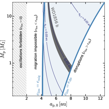
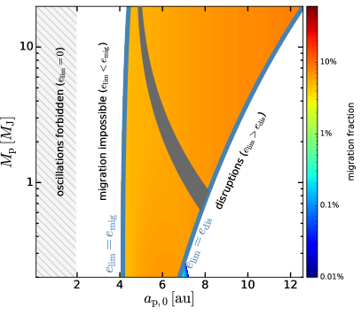
Figure 1: Kozai migration paths in the WD 1856+534 system. Left panel: regions of viable migration with thin dark blue contours depicting $a_{\rm p,f}$ (Equation 2a) and thin light blue contours depicting the boundaries of migration ($e_{\rm lim}=e_{\rm mig}$, left) and disruption ($e_{\rm lim}=e_{\rm diss}$, right) (Equation 2b). The cross-hatched region corresponds complete quenching of ZLK oscillations owing to GR ($\varepsilon_{\rm GR}\geq 9/8$; Equation 4) and the dark gray region depicts the current semi-major axis of WD 1856b (Table 1). Right panel: Kozai migration fractions calculated by the analytical method of Muñoz et al. (2016). Within the migration boundaries, the migration rate is $\sim 5\%$, and is primarily given by the with of the octupole window (Equation 6), except for a small region at small planet mass and $a_{\rm p,0}\simeq 7$, where the quadrupole window can also lead to migrations.

At the quadrupole-level of approximation, the value of $e_{\rm max}$ grows monotonically with $i_{0}$ until it reaches its upper bound, or “limiting eccentricity” $e_{\rm lim}$, when $\cos i_{0}=0$. Typically, $e_{\rm max}$ will not surpass the critical value $e_{\rm mig}$ unless $i_{0}$ is very close to $90^{\circ}$. This narrow range of inclinations, $[90^{\circ}{-}\Delta i_{\rm quad},90^{\circ}{+}\Delta i_{\rm quad}]$, subtends a solid angle $\sin\Delta i_{\rm quad}$ that equals the fraction of orbital orientations in the unit sphere that lead to migrations/disruptions (Muñoz et al., 2016).

At the octupole-level of approximation, however, a wider range of initial inclinations can reach extreme eccentricities (Katz et al., 2011), with all angles within the “octupole window” $[90^{\circ}{-}\Delta i_{\rm quad},90^{\circ}{+}\Delta i_{\rm quad}]$ reaching $e_{\rm max}\approx e_{\rm lim}$ (Liu et al., 2015). The width of the window is

$$\Delta i_{\rm oct}\approx 2.9^{\circ}\left(\frac{\varepsilon_{\rm oct}}{10^{-3}}\right)^{1/2}$$ (6)

(Muñoz et al., 2016) where $\varepsilon_{\rm oct}=(a_{\rm p,0}/a_{\rm out})e_{\rm out}(1-e_{\rm out}^{2})^{-1}$ is the octupole strength parameter (e.g. Ford et al., 2000; Lithwick & Naoz, 2011; Naoz, 2016), which vanishes for non-eccentric outer companions. For the system WD 1856+534/G 220-20 AB, we have $\varepsilon_{\rm oct}\approx 1.1\times 10^{-3}(a_{\rm p,0}/5{\rm au})$. While small, this value of $\varepsilon_{\rm oct}$ is large enough to provide an octupole window of $\simeq 3^{\circ}$, which covers a solid angle of $\simeq 0.05$, implying that about $5\%$ of planets will undergo extreme eccentricity excursions.

In most cases of interest, the octupole window is wider than its quadrupole counterpart, which allows us to replace $e_{\rm max}(a_{\rm p,0},M_{\rm p},i_{0})$ with $e_{\rm lim}(a_{\rm p,0},M_{\rm p})$ in Equations (2), effectively relegating $i_{0}$ to a secondary role, provided that the system is inside the octupole window. By making this simplification, we reduce the number of unknowns to only two. For each $(a_{\rm p,0},M_{\rm p})$ pair, we can compute $e_{\rm lim}$, and then derive a unique value of $a_{\rm p,f}\approx 2a_{\rm p}[1-e_{\rm lim}(a_{\rm p,0},M_{\rm p})]$. In turn, $e_{\rm lim}$ is solved from:

$$\begin{split}0=&\frac{9}{8}{e_{\rm lim}^{2}}-\varepsilon_{\rm GR}\bigg{[}\frac{1}{(1-e_{\rm lim}^{2})^{1/2}}-1\bigg{]}\\ &-\frac{\varepsilon_{\rm tide}}{15}\bigg{[}\frac{1+3e^{2}_{\rm lim}+\frac{3}{8}e^{4}_{\rm lim}}{(1-e_{\rm lim}^{2})^{9/2}}-1\bigg{]}~{}.\end{split}$$ (7)

We illustrate this calculation in Figure 1 (left panel), where the dark blue contours show levels of constant $a_{\rm p,f}$ for different values of of $a_{\rm p,0}$ and $M_{\rm p}$. The tight constraints imposed on $a_{\rm p}$ by Vanderburg et al. (2020) (gray band) translate into a tight correlation between the values of $a_{\rm p,0}$ and $M_{\rm p}$ that can explain this system.

2.2 High-e Migration within a Cooling Time

The migration condition (2b) requires explicit definitions of $e_{\rm mig}$ and $e_{\rm dis}$ (e.g., Muñoz et al., 2016). The first of these comes from the requirement that migration must be completed on timescales shorter than the cooling age of the WD. Thus, we require $\tau_{\rm dec}^{\rm(ST)}\lesssim T_{\rm cool}$, where

$$\tau_{\rm dec}^{\rm(ST)}=\frac{0.357}{k_{2p}\Delta t_{L}}\frac{M_{\rm p}}{\mathcal{G}M_{*}^{2}}\frac{a_{0}^{8}~{}(1-e_{\rm max})^{7}}{R_{\rm p}^{5}}$$ (8)

is the orbital decay timescale due to high-eccentricity excursions (e.g. Anderson et al., 2016) and where ‘ST’ stands for the ‘standard tides’ of weak friction theory (e.g. Alexander, 1973; Hut, 1981). Solving for the eccentricity, we obtain the minimum eccentricity required for migration

$$e_{\rm mig}\equiv 1-1.96\left(\frac{k_{2{\rm p}}\Delta t_{L}T_{\rm cool}}{P_{\rm p,0}^{2}}\frac{M_{\rm WD}}{M_{\rm p}}\frac{R_{\rm p}^{5}}{a_{\rm p,0}^{5}}\right)^{1/7}~{}.$$ (9)

Similarly, we define an eccentricity above which disruption takes place

$$e_{\rm dis}\equiv 1-\eta_{\rm dis}\frac{R_{\rm p}}{a_{\rm p,0}}\left(\frac{M_{\rm WD}}{M_{\rm p}}\right)^{1/3}$$ (10)

where $\eta_{\rm dis}=2.7$ (Guillochon et al., 2011).

The two limits, $e_{\rm lim}=e_{\rm mig}$ and $e_{\rm lim}=e_{\rm dis}$, are overlaid into Figure 1 (left panel) as light blue curves. Migration is only possible these boundaries. This additional requirement further constraints the mass and original semimajor of the WD 1856 b: $M\gtrsim 0.7M_{\rm J}$ and $5~{}\text{au}\lesssim a_{\rm p,0}\lesssim 8~{}\text{au}$.

The slope of the migration and disruption limits can be understood analytically. When $e_{\rm lim}\approx 1$, Equation (3) can be simplified further (see eq. 57 of Liu et al., 2015), which allows us to define ‘tide-dominated’ and ‘GR-dominated’ limits to $e_{\rm lim}$. Thus, when approaching the tidal disruption limit $1-e_{\rm lim}^{2}\approx({7\varepsilon_{\rm Tide}}/{27})^{2/9}$, for which $e_{\rm lim}=e_{\rm dis}$ implies

$$\begin{split}&a_{\rm p,0}^{\rm(dis)}\simeq 8.4~{}{\rm au}~{}\left[\frac{a_{\rm out}\sqrt{1-e_{\rm out}^{2})}}{1500~{}{\rm au}}\right]^{6/7}\left[\frac{\eta_{\rm dis}}{2.7}\right]^{-9/7}\left[\frac{R_{\rm p}}{R_{\rm J}}\right]^{1/7}\\ &\times\left[\frac{k_{2p}}{0.37}\right]^{2/7}\left[\frac{M_{\rm p}}{M_{\rm J}}\right]^{1/7}\left[\frac{M_{\rm WD}}{0.5M_{\odot}}\right]^{1/7}\left[\frac{M_{\rm out}}{0.7M_{\odot}}\right]^{-2/7}\end{split}$$ (11)

Conversely, when approaching the migration limit, $1-e_{\rm lim}^{2}\approx({8\varepsilon_{\rm GR}}/{9})^{2}$, and thus, when $e_{\rm lim}=e_{\rm mig}$ we have

$$\begin{split}&a_{\rm p}^{\rm(mig)}=4.36~{}{\rm au}~{}(k_{2{\rm p}}\chi{\cal T})^{-1/48}\left[\frac{a_{\rm out}\sqrt{1-e_{\rm out}^{2}}}{1500~{}{\rm au}}\right]^{7/8}\\ &\times\left[\frac{R_{\rm p}}{R_{\rm J}}\right]^{-5/48}\left[\frac{M_{\rm WD}}{0.5M_{\odot}}\right]^{13/24}\left[\frac{M_{\rm out}}{0.7M_{\odot}}\right]^{-7/24}\left[\frac{M_{\rm p}}{M_{\rm J}}\right]^{1/48}\end{split}$$ (12)

where $\chi=\Delta t_{L}/0.1{\rm s}$ and ${\cal T}=T_{\rm cool}/1{\rm Gyr}$. From these analytical expressions, we see that the dependence of $a_{\rm p}^{\rm(mig)}$ and $a_{\rm p}^{\rm(dis)}$ is weak on most parameters except for $a_{\rm out}$, which underscores the importance of having a well characterized outer orbit when estimating the migration viability and the migration fraction.

Migration Fractions

In Figure 1 (right panel), we compute the Kozai migration fraction around WD 1856+534 following the approximated method of Muñoz et al. (2016). The figure shows that the migration rate is vastly dominated by the octupole window (except at $a_{\rm p,0}\sim 7$ au and $M_{\rm p}\lesssim 0.2M_{\rm J}$), which results in a migration rate given by the solid angle $\sin\Delta i_{\rm oct}\approx 5\%$ regardless of planet mass and initial semi-major axis.

2.2.1 Fast Migration and Chaotic Tides

The approximate method laid out above implicitly assumes that the dissipation rate is low enough such that the energy is conserved over the ZLK timescale $\tau_{\rm quad}$, and that dissipation does not preclude $e_{\rm lim}$ from being reached. In principle, however, and under highly dissipative conditions, enough orbital energy can be lost during just one ZLK cycle to decouple the planet from the companion’s tidal field, halting subsequent oscillations. This regime –referred to as “fast migration” by Petrovich (2015)– can cap the maximum eccentricity to some value $e_{\rm fast}^{\rm(ST)}$ and shield planets from being tidally disrupted if $e_{\rm fast}^{\rm(ST)}<e_{\rm dis}$. In most cases, however, $e_{\rm fast}^{\rm(ST)}$ is not low enough to prevent disruption, unless unrealistically large values of $\Delta t_{L}$ are used (Petrovich, 2015).

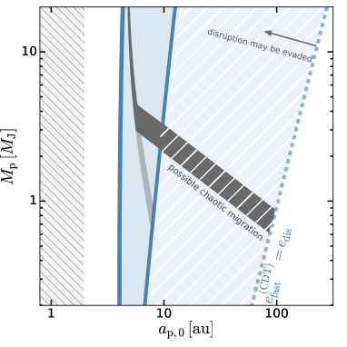
Figure 2: Same as Figure 1 (left panel), but after replacing $e_{\rm lim}$ with $\min[e_{\rm lim},e_{\rm fast}^{\rm(CDT)}]$ (Equation 14) to take chaotic tides into account (Section 2.2.1). The cross-hatched area highlights the region in which disruption may be evaded by chaotic tides and migration is possible; this region is probabilistic, with both disruptions and migrations taking place in roughly equal fractions (Vick et al., 2019).

An analogous, yet more efficient, effect can be accomplished via chaotic dynamical tides (e.g. Mardling, 1995; Vick & Lai, 2018; Wu, 2018). In this mechanism, the planet’s fundamental mode of oscillation is erratically excited/reduced at each pericenter passage. The mode can grow stochastically until it “breaks”, dissipating a significant amount of energy. The CDT dissipation timescale is given by

$$\tau_{\rm dec}^{\rm(CDT)}=\pi\frac{M_{\rm p}\sqrt{{\cal G}M_{\rm WD}a_{\rm p,0}}}{\Delta E_{\alpha}}~{},\;\;\;\;\Delta E_{\alpha}=\frac{{\cal G}M_{\rm p}^{2}}{R_{\rm p}}\eta^{-6}T_{22}$$ (13)

where $\eta\equiv(a_{\rm p,0}/R_{\rm p})(M_{\rm p}/M_{\rm WD})^{1/3}(1-e)$ and $\Delta E_{\alpha}$ is the amount energy injected into the f-mode that is dissipated (e.g., Lai, 1997) and $T_{22}$ is a dimensionless function (Press & Teukolsky, 1977). Using values derived by Vick et al. (2019) for a polytropic model of a gas, we can approximate $T_{22}\approx 2\times 10^{3}\eta^{-10}$ for $\eta\gtrsim\eta_{\rm dis}=2.7$. The requirement for fast migration, just like in the ‘standard tides’ case, stems from the requiring that $\tau_{\rm dec}$ is shorter than the time spent above an eccentricity $e$ during ZLK oscillations, i.e., $\tau_{\rm dec}\lesssim\tau_{\rm quad}\sqrt{1-e_{\rm max}^{2}}$ (e.g., Anderson et al., 2016). Solving for the eccentricity, we find

$$\begin{split}e_{\rm fast}^{\rm(CDT)}\gtrsim 1-1.55\bigg{[}&\left(\frac{R_{\rm p}}{a_{\rm p,0}}\right)^{15}\left(\frac{M_{\rm WD}}{M_{\rm p}}\right)^{13/3}\frac{M_{\rm WD}}{M_{\rm out}}\\ &\times\left(\frac{a_{\rm out}}{a_{\rm p,0}}\right)^{3}(1-e_{\rm out}^{2})^{3/2}\bigg{]}^{2/31}~{}.~{}~{}~{}~{}~{}~{}~{}~{}~{}~{}~{}~{}~{}~{}~{}~{}~{}~{}\end{split}$$ (14)

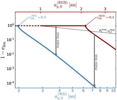
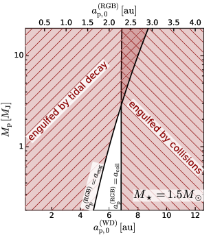
Figure 3: ZLK oscillations in the RGB phase. Left panel: modification of $e_{\rm lim}$ after a change in $\varepsilon_{\rm GR}$ triggered by mass loss between the RGB (red) and WD (blue) phases (Equation 15). The RGB phase exhibits fully quenched ZLK for $a_{\rm p,0}^{\rm(RGB)}\lesssim 2.15$ (when $\epsilon_{\rm GR}^{\rm(RGB)}=9/4$); this region is awakened after a mass change of $1M_{\odot}$, exposing all planets with $a_{\rm p,0}^{\rm(WD)}\gtrsim 0.68$ to ZLK oscillations. For reference, we also depict $R_{\star}^{\rm(RGB)}/a_{\rm p,0}^{\rm(RGB)}$ which intersec $1-e_{\rm lim}$ at 2.3 au (Equation 17). Right panel: planet survival during the RGB phase. Semimajor axes greater than $a_{\rm coll}\approx 2.3$ au get too eccentric to survive collision with the inflated stellar envelope. Semimajor axes smaller than the $a_{\rm p}\propto M_{\rm p}^{1/8}$ line decay because of tides in the star (e.g., Villaver et al., 2014). The white region is the only one that survives at high inclinations.

In Figure 2, we repeat the calculation leading to Figure 1, but replacing $e_{\rm lim}\rightarrow\min[e_{\rm lim},e_{\rm fast}^{\rm(CDT)}]$. The effect of chaotic tides is readily appreciated by the dramatic shift of the disruption boundary toward much larger initial semi-major axes (see fig. 10 in Vick et al., 2019), seemingly expanding the parameter space of orbits that could explain WD 1856 b (cross-hatched region). Within this greatly expanded parameter space, the migration condition $a_{\rm p,f}=0.02$ au (Equation 2) constrains the planet mass within a factor of 2, but at the expense of a highly uncertain initial semi-major axis. Fortunately, the true viability of this expanded region is severely limited if we additionally require planets to have survived earlier phases of stellar evolution. Below, we show that survival during the RGB largely rules out the chaotic tide domain.

3 Pre-WD phase

Having shown that WD 1856 b could have successfully migrated via ZLK oscillations from much larger separations, we now turn to addressing if such a planet could have orbited a WD in the first place, having survived the MS and the subsequent giant phases.

3.1 Quenched ZLK Oscillations Before Mass Loss

It is known that mass loss can awaken “dormant” secular instabilities in triples and multiples. The driver behind this awakening is the unequal expansion of the orbits. For example, in the so-called ‘mass-loss induced eccentric Kozai’ (MIEK) mechanism (Shappee & Thompson, 2013), $\epsilon_{\rm oct}{\propto}a_{\rm p,0}/a_{\rm out}$ grows, and alongside it, so does the width of the octupole window (Equation 6), which can promote mild eccentricity oscillations into extreme ones.

Similarly, the expansion of the semi-major axes due to mass loss changes the balance of short-range forces in Equation (7). If a star of mass $M_{\star}$ loses an amount $\Delta M$ adiabatically, then the semi-major axis of the planet changes as $a_{\rm p}{\rightarrow}a_{\rm p}M_{\star}/(M_{\star}-\Delta M)$, while that of the binary changes as $a_{\rm out}{\rightarrow}a_{\rm out}(M_{\star}+M_{\rm out})/(M_{\star}{+}M_{\rm out}{-}\Delta M)$. Consequently, the GR coefficient changes by an amount

$$\varepsilon_{\mathrm{GR}}\rightarrow\varepsilon_{\mathrm{GR}}\frac{(M_{\star}-\Delta M)^{6}}{M_{\star}^{6}}\frac{(M_{\star}+M_{\rm out})^{3}}{(M_{\star}{+}M_{\rm out}{-}\Delta M)^{3}}~{},$$ (15)

which modifies the moderating or quenching effect that GR exerts on ZLK oscillations. The change in the GR coefficient is significant if we consider the mass loss rates of G, F and A stars toward the end of their respective AGB phases. With $\Delta M\simeq 0.5-1.5M_{\odot}$ for WD 1856+534 (Cummings et al., 2018), the respective change in $\varepsilon_{\rm GR}$ is $\simeq 0.05-0.003$. We further illustrate this effect in Figure 3, were we depict $e_{\rm lim}$ (Equation 7) as a function of planet semi-major axis before and after mass loss.

3.2 Surviving the RGB phase

The RGB phase of stellar evolution imperils any planet orbiting at a distance of a few au, compromising the planet’s chances of surviving all the way to the WD phase. These planets are directly affected by the inflated stellar envelope in two ways. First, by stellar tides: the greatly expanded star makes it susceptible to planet-induced tides, which can shrink the orbit effectively, leading to engulfment if

$$a_{\rm p}^{\rm(RGB)}\leq a_{\rm eng}\equiv 2\mbox{ au }\left(\frac{M_{\rm p}}{1M_{\rm J}}\right)^{1/8}~{}$$ (16)

(e.g. Villaver et al., 2014), where $a_{\rm p}^{\rm(RGB)}$ denotes the planet semi-major axis during the RGB phase. We caution that this boundary is fuzzy and highly dependent on the tidal model.

And second, by direct high-eccentricity collisions: in the presence of a binary companion, ZLK oscillations can lead to the planet being engulfed by directly plunging it into the stellar envelope; this condition reads

$$a_{\rm p}^{\rm(RGB)}\leq a_{\rm coll}\equiv R_{\star}^{\rm(RGB)}(1-e_{\rm lim}^{\rm(RGB)})^{-1}$$ (17)

where $R_{\star}^{\rm(RGB)}\simeq 1$ au is the maximum radius reached by the stellar envelope in the RGB phase (e.g., Villaver et al., 2014), and where $e_{\rm lim}^{\rm(RGB)}$ is the solution to Equation (7) evaluated with parameters appropriate for the RGB phase at peak radius.

The joint requirement $a_{\rm eng}<a_{\rm p}^{\rm(RGB)}<a_{\rm coll}$ guarantees survival of planets throughout the RGB phase. As it turns out, this condition is difficult to satisfy, and a large fraction of $a_{\rm p}^{\rm(RGB)}{-}M_{\rm p}$ space is excluded (Figure 3, right panel). The engulfment condition (Equation 16) and the collision condition (Equation 17) conspire to create a narrow region (in white) that allows inclined planets to survive.

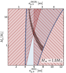
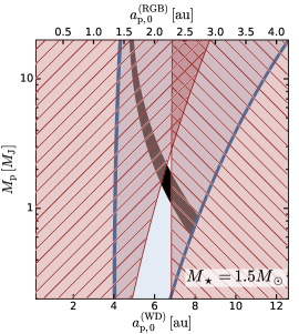
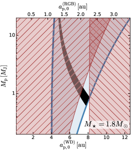
Figure 4: Survival and migration viability of highly inclined planets throughout stellar evolution. We combine the requirements Figures 1 and 3 (right panel) to constrain the initial conditions of WD 1856 b for different values of the initial stellar mass $M_{\star}$. The F star (left panel) does not survival and migration; the late A star (middle panel) allows for survival and migration via standard tides, the early A star (right panel) may allow for survival and migration via chaotic tides.

We are now in a position to combine the migration viability conditions of Figure 1 with the survival conditions of Figure 3 (right panel), to identify which regions of parameter space give WD 1856 b a viable path to its current orbit. We show these overlaid conditions in Figure 4 for different values of $M_{\star}$ –the initial stellar mass. This figure shows that if $M_{\star}\leq 1.3M_{\odot}$ (left panel) there is no possible path for WD 1856 b to have survived and migrated. Conversely, there is a narrow range of parameters that explains WD 1856 b’s current orbit if $M_{\star}\simeq 1.5-1.8~{}M_{\odot}$ (middle and right panels), which roughly corresponds to $M_{\rm p}\simeq 0.7-3M_{\rm J}$ and $a_{\rm p,0}=2-2.5a_{\rm p,0}$.

At even higher initial stellar masses, the survival region overlaps with that dominated by disruptions and/or chaotic tides (Section 2.2.1). Initial masses above $1.8M_{\odot}$, however, are unlikely to produce WD 1856+534 (Cummings et al., 2018), indicating that chaotic tides play a minor role, if any, in enabling planets with $a_{\rm p,0}\sim 2.5$ au to be precursors of WD 1856 b.

4 Discussion

We have demonstrated that Kozai migration can explain the recent discovery of the planet-size companion to WD 1856+534. By simultaneously requiring that the companion is not lost prematurely during the RGB phase and that it subsequently migrates to its current location, we are able to constrain the planet’s initial semi-major axis ($\simeq 2-2.5$ au) and mass ($\simeq 0.7-3M_{\rm J}$).

4.1 Occurrence rate

To provide with an estimate of the occurrence rate of WD-transiting Jovians, we proceed as follows. We assume that the progenitor is always an A star. The binarity fraction of A-type stars is ${\cal F}_{\rm bin}\simeq 0.7$ (De Rosa et al., 2014) and their giant planet-bearing fraction is ${\cal F}_{\rm Jup}\simeq 0.2$ (Ghezzi et al., 2018). We assume that the semi-major axes $a_{\rm p}$ and $a_{\rm out}$, and the mutual inclination $i_{0}$ follow independent distributions. We then define the fraction of systems that survive stellar evolution and subsequently migrate into a close-in orbit as

$${\cal F}_{\rm surv,mig}=\int d\log a_{p}d\log a_{\rm out}d\cos i_{0}\frac{dN}{d\log a_{\rm p}}\frac{dN}{d\log a_{\rm out}}$$

$$\times \Theta\left[a_{\rm p}-2\mbox{ au}\right]\times\Theta\left[(1-e_{\rm lim}^{\rm(RGB)})-R_{\star}^{\rm(RGB)}/a_{p}\right]$$

$$\times \Theta\left[2R_{\odot}/a_{p}^{\rm(WD)}-(1-e_{\rm lim}^{\rm(WD)})\right]\times\Theta[2.6\varepsilon_{\rm oct}^{\rm(WD)}-\cos^{2}i_{0}],$$

where $\Theta$ is the Heaviside function. The last term in the integral represents the effects of the octupole window (Equation 6).

We evaluate ${\cal F}_{\rm surv,mig}$ assuming log-normal distributions in the semi-major axes: $\ln(a_{\rm p,0}/{\rm au})\sim{\cal N}(0.92,0.7)$ and $\ln(a_{\rm out}/{\rm au})\sim{\cal N}(5.97,0.78)$, in broad agreement with Fernandes et al. (2019) and De Rosa et al. (2014), respectively. For simplicity, we assume that all wide binary companions have $e_{\rm out}=2/3$. This yields ${\cal F}_{\rm surv,mig}\simeq 0.3\%$.

The net fraction of WDs hosting close-in Jovians owing to Kozai migration is

$${\cal F}_{\rm WD,Jup} = {\cal F}_{\rm Jup}\times{\cal F}_{\rm b}\times{\cal F}_{\rm surv,mig}$$ (19)

$$\simeq 0.2\times 0.7\times 0.003\simeq 4\times 10^{-4}$$

or one planet per $\simeq 2,500$ WDs, which is consistent with the $3-\sigma$ upper limits of $0.45\%$ derived from photometric surveys (Fulton et al., 2014; van Sluijs & Van Eylen, 2018). However, we cannot rule out other migration mechanisms that could increase ${\cal F}_{\rm WD,Jup}$. For example, the gas giant around WD 1145+017 (Gänsicke et al., 2019) is too young ($\sim 13$ Myr), and its orbital separation too wide ($\sim 0.07$ au), to be explained by Kozai migration (Veras & Fuller, 2020).

Further constraints on the occurrence of close-in Jupiters around WDs are expected in the near future from various surveys, including LSST with expected yields of $10^{7}$ surveyed WDs (Agol, 2011). With a detectability of $\simeq 2\%$ for WD 1856b-like planets (Cortés & Kipping, 2019), we expect $\sim 100$ Kozai-migrated planets to be discovered in the the ten year baseline of LSST.

4.2 Increasing Occurrence with Additional Effects

The main bottleneck in the low occurrence rate is the joint requirement of past survival plus a late-onset migration, which severely restricts the viable region of parameter space (Figure 4). These calculations, however, are sensitive to the choices of $a_{\rm eng}$ and $a_{\rm coll}$ (Equations 16 and 17), as well as the disruption boundary (Equation 11), and are thus subject to caveats.

A way of expanding the survival window (Figure 3, right panel) is to incorporate additional sources of apsidal precession to shift the $a_{\rm p}^{\rm(RGB)}=a_{\rm coll}$ boundary to the right. This effect can be accomplished by adding a planetary system interior to $\sim 2$ au, as proposed by Petrovich & Muñoz (2017). Additional planets quench ZLK oscillations, which can be triggered once the planets are engulfed in the RGB or AGB phases (see Ronco et al. 2020 for engulfment in multi-planet systems).

4.3 Relation to Previous Work

In this work, we have used mass loss to trigger an otherwise suppressed ZLK mechanism. Delaying the onset of ZLK oscillations was instrumental for constraining the past and present properties of WD 1856 b. More generally, though, mass loss can trigger varied responses (e.g., Kratter & Perets, 2012; Veras et al., 2013), and it can lead to dynamical and secular instabilities that are effective at transporting material/minor bodies toward the WD when binaries are present (see Veras 2016 for a review).

One such possibility is the enhanced effect of galactic tides for very wide binaries ($\gtrsim 5000$ au). The galactic tide that can make $e_{\rm out}$ grow within a cooling age, thus disturbing a planetary system (Bonsor & Veras, 2015). In the case of WD 1856+534, however, the outer companions are too close for the galactic tide to operate.

A second possibility is the MIEK mechanism discussed above, which produces the widening the "octupole window", promoting conventional (quadrupolar) ZLK oscillations into extreme (octupolar) ones (Shappee & Thompson, 2013; Hamers & Portegies Zwart, 2016; Stephan et al., 2017). But the applicability of this mechanism is limited in the case of WD 1856+534, because the octupole window is known to be narrow ($\simeq 3^{\circ}$), even after being widened by mass loss. If planets were to be promoted into octupolar oscillations, it would be from already large inclinations, which would accompanied by large amplitude (quadrupolar) oscillations during the MS and RGB phases. Consequently, in order to survive the RGB phase, these planets would need to start from very large initial semi-major axes ($\sim$100 au), like in the simulations of Hamers & Portegies Zwart (2016) and Stephan et al. (2017). The scarcity of Jovians planets at such large distances from the host star (Fernandes et al., 2019) renders this type of mechanism improbable.

4.3.1 Dynamics of 2+2 Systems

We have treated the outer M-dwarf binary as single body of mass $M_{\rm out}=M_{A}+M_{B}$. This approximation may break-down in some regimes, especially when the quadrupolar field from the double M-dwarf modulates the wide binary on timescales comparable to $\tau_{\rm quad}$. Under certain conditions, the quadruple system can evolve chaotically, with the eccentricity diffusively evolving toward extreme values (Hamers & Lai, 2017). In the WD 1856+534 system and $a_{\rm p,0}\simeq 5-8$ au, however, the dimensionless quantity

$$\frac{3}{4}\left(\frac{M_{\rm WD}}{M_{\rm out}}\right)^{3/2}\left(\frac{a_{\rm AB}}{a_{p}}\right)^{3/2}\sim 10-28$$ (20)

is too large for this chaotic diffusion to operate, and we can thus safely treat the system as a triple. It is nonetheless worthy of mention that mass loss can increase Equation (20), and conceivably activate the chaotic 2+2 dynamics for some systems with larger semi-major axes ($a_{\rm p,0}\sim a_{\rm AB}$) after a WD is formed.

5 Conclusion

We have shown that the current orbit of WD 1856 b can be explained with Kozai migration without any ad hoc requirements other than a highly inclined orbit respect to the outer companions. By requiring that WD 1856 b survived stellar evolution and that its migration began during the WD phase, we are able to constrain its initial semi-major axis and mass. We infer an initial separation of $2-2.5$ au, and a mass of $0.7-3M_{\rm J}$, implying that WD 1856 b was born a typical gas giant.

Although the initial conditions we have derived are typical of planetary systems, the planets that survive till the end of the WD phase are rare. We predict the occurrence rate of close-in Jovians from Kozai migration around WDs to be ${\cal O}(10^{-3}{-}10^{-4})$ and expect that LSST will find ${\sim}100$ of such systems.

References

- Agol (2011) Agol, E. 2011, ApJ, 731, L31, doi: 10.1088/2041-8205/731/2/L31
- Alexander (1973) Alexander, M. E. 1973, Ap&SS, 23, 459, doi: 10.1007/BF00645172
- Anderson et al. (2016) Anderson, K. R., Storch, N. I., & Lai, D. 2016, MNRAS, 456, 3671, doi: 10.1093/mnras/stv2906 nord
- Bonsor & Veras (2015) Bonsor, A., & Veras, D. 2015, MNRAS, 454, 53, doi: 10.1093/mnras/stv1913
- Cortés & Kipping (2019) Cortés, J., & Kipping, D. 2019, MNRAS, 488, 1695, doi: 10.1093/mnras/stz1300
- Cummings et al. (2018) Cummings, J. D., Kalirai, J. S., Tremblay, P. E., Ramirez-Ruiz, E., & Choi, J. 2018, ApJ, 866, 21, doi: 10.3847/1538-4357/aadfd6
- De Rosa et al. (2014) De Rosa, R. J., Patience, J., Wilson, P. A., et al. 2014, MNRAS, 437, 1216, doi: 10.1093/mnras/stt1932
- Fabrycky & Tremaine (2007) Fabrycky, D., & Tremaine, S. 2007, ApJ, 669, 1298, doi: 10.1086/521702
- Fernandes et al. (2019) Fernandes, R. B., Mulders, G. D., Pascucci, I., Mordasini, C., & Emsenhuber, A. 2019, ApJ, 874, 81, doi: 10.3847/1538-4357/ab0300
- Ford et al. (2000) Ford, E. B., Kozinsky, B., & Rasio, F. A. 2000, ApJ, 535, 385, doi: 10.1086/308815
- Fulton et al. (2014) Fulton, B. J., Tonry, J. L., Flewelling, H., et al. 2014, ApJ, 796, 114, doi: 10.1088/0004-637X/796/2/114
- Gänsicke et al. (2019) Gänsicke, B. T., Schreiber, M. R., Toloza, O., et al. 2019, Nature, 576, 61, doi: 10.1038/s41586-019-1789-8
- Ghezzi et al. (2018) Ghezzi, L., Montet, B. T., & Johnson, J. A. 2018, ApJ, 860, 109, doi: 10.3847/1538-4357/aac37c
- Guillochon et al. (2011) Guillochon, J., Ramirez-Ruiz, E., & Lin, D. 2011, ApJ, 732, 74, doi: 10.1088/0004-637X/732/2/74
- Hamer & Schlaufman (2020) Hamer, J. H., & Schlaufman, K. C. 2020, AJ, 160, 138, doi: 10.3847/1538-3881/aba74f
- Hamers & Lai (2017) Hamers, A. S., & Lai, D. 2017, MNRAS, 470, 1657, doi: 10.1093/mnras/stx1319
- Hamers & Portegies Zwart (2016) Hamers, A. S., & Portegies Zwart, S. F. 2016, MNRAS, 462, L84, doi: 10.1093/mnrasl/slw134
- Howard et al. (2012) Howard, A. W., Marcy, G. W., Bryson, S. T., et al. 2012, ApJS, 201, 15, doi: 10.1088/0067-0049/201/2/15
- Hut (1981) Hut, P. 1981, A&A, 99, 126
- Ito & Ohtsuka (2019) Ito, T., & Ohtsuka, K. 2019, Monographs on Environment, Earth and Planets, 7, 1, doi: 10.5047/meep.2019.00701.0001
- Katz et al. (2011) Katz, B., Dong, S., & Malhotra, R. 2011, Phys. Rev. Lett., 107, 181101, doi: 10.1103/PhysRevLett.107.181101
- Kozai (1962) Kozai, Y. 1962, AJ, 67, 591, doi: 10.1086/108790
- Kratter & Perets (2012) Kratter, K. M., & Perets, H. B. 2012, ApJ, 753, 91, doi: 10.1088/0004-637X/753/1/91
- Lai (1997) Lai, D. 1997, ApJ, 490, 847, doi: 10.1086/304899
- Lidov (1962) Lidov, M. L. 1962, Planet. Space Sci., 9, 719, doi: 10.1016/0032-0633(62)90129-0
- Lithwick & Naoz (2011) Lithwick, Y., & Naoz, S. 2011, ApJ, 742, 94, doi: 10.1088/0004-637X/742/2/94
- Liu et al. (2015) Liu, B., Muñoz, D. J., & Lai, D. 2015, MNRAS, 447, 747, doi: 10.1093/mnras/stu2396
- Mardling (1995) Mardling, R. A. 1995, ApJ, 450, 732, doi: 10.1086/176179
- McCook & Sion (1999) McCook, G. P., & Sion, E. M. 1999, ApJS, 121, 1, doi: 10.1086/313186
- Muñoz et al. (2016) Muñoz, D. J., Lai, D., & Liu, B. 2016, MNRAS, 460, 1086, doi: 10.1093/mnras/stw983
- Naoz (2016) Naoz, S. 2016, ARA&A, 54, 441, doi: 10.1146/annurev-astro-081915-023315
- Naoz et al. (2012) Naoz, S., Farr, W. M., & Rasio, F. A. 2012, ApJ, 754, L36, doi: 10.1088/2041-8205/754/2/L36
- Petrovich (2015) Petrovich, C. 2015, ApJ, 799, 27, doi: 10.1088/0004-637X/799/1/27
- Petrovich & Muñoz (2017) Petrovich, C., & Muñoz, D. J. 2017, ApJ, 834, 116, doi: 10.3847/1538-4357/834/2/116
- Press & Teukolsky (1977) Press, W. H., & Teukolsky, S. A. 1977, ApJ, 213, 183, doi: 10.1086/155143
- Ronco et al. (2020) Ronco, M. P., Schreiber, M. R., Giuppone, C. A., et al. 2020, ApJ, 898, L23, doi: 10.3847/2041-8213/aba35f
- Shappee & Thompson (2013) Shappee, B. J., & Thompson, T. A. 2013, ApJ, 766, 64, doi: 10.1088/0004-637X/766/1/64
- Stephan et al. (2018) Stephan, A. P., Naoz, S., & Gaudi, B. S. 2018, AJ, 156, 128, doi: 10.3847/1538-3881/aad6e5
- Stephan et al. (2017) Stephan, A. P., Naoz, S., & Zuckerman, B. 2017, ApJ, 844, L16, doi: 10.3847/2041-8213/aa7cf3
- van Sluijs & Van Eylen (2018) van Sluijs, L., & Van Eylen, V. 2018, MNRAS, 474, 4603, doi: 10.1093/mnras/stx3068
- Vanderburg et al. (2020) Vanderburg, A., Rappaport, S. A., Xu, S., et al. 2020, arXiv e-prints, arXiv:2009.07282. https://arxiv.org/abs/2009.07282
- Veras (2016) Veras, D. 2016, Royal Society Open Science, 3, 150571, doi: 10.1098/rsos.150571
- Veras & Fuller (2020) Veras, D., & Fuller, J. 2020, MNRAS, 492, 6059, doi: 10.1093/mnras/staa309
- Veras et al. (2013) Veras, D., Mustill, A. J., Bonsor, A., & Wyatt, M. C. 2013, MNRAS, 431, 1686, doi: 10.1093/mnras/stt289
- Vick & Lai (2018) Vick, M., & Lai, D. 2018, MNRAS, 476, 482, doi: 10.1093/mnras/sty225
- Vick et al. (2019) Vick, M., Lai, D., & Anderson, K. R. 2019, MNRAS, 484, 5645, doi: 10.1093/mnras/stz354
- Villaver et al. (2014) Villaver, E., Livio, M., Mustill, A. J., & Siess, L. 2014, ApJ, 794, 3, doi: 10.1088/0004-637X/794/1/3
- von Zeipel (1910) von Zeipel, H. 1910, Astronomische Nachrichten, 183, 345, doi: 10.1002/asna.19091832202
- Wu (2018) Wu, Y. 2018, AJ, 155, 118, doi: 10.3847/1538-3881/aaa970
- Wu & Murray (2003) Wu, Y., & Murray, N. 2003, ApJ, 589, 605, doi: 10.1086/374598