The effective fluid approach for modified gravity

Abstract

Current and coming surveys will require sub-percent agreement in theoretical accuracy to test the different cosmological and gravity scenarios. This can be performed with Boltzmann solvers, i.e. codes that solve the linear evolution of cosmological perturbations. Given the plethora of gravity models, it is crucial to have a standardized unified way to describe all of them and take them into account in a Boltzmann code. Dark Energy (DE) and Modified Gravity (MG) models, although at a first glance quite dissimilar, are possible to unify them within the same framework. In this paper we present a scenario, based on the effective fluid approach that allows to map any modified gravity model as an effective dark energy fluid and then we show how to implement it into existing Boltzmann codes in a simple and straightforward way. This approach has also the advantage that only a handful of variables are needed to compute, i.e the equation of state $w(a)$ at the background level and the sound speed $c_{s}^{2}(a,k)$ and the anisotropic stress $\pi(a,k)$ at the linear perturbation. In particular we show that with simple modifications to the latter Cosmic Linear Anisotropy Solving System (CLASS) code, which we called EFCLASS, we provide competitive results in a much simpler and less error-prone approach in including the effects of modified gravity models. To test our modifications, we particularize the effective fluid approach to f(R) theories and a surviving class of Horndeski models, the designer Horndeski (HDES) which have a background exactly to the standard cosmological model $\Lambda$CDM.

I Introduction

The standard cosmological model $\Lambda$CDM, which is in very good agreement with all of the current data from surveys Aghanim et al. (2018); Abbott et al. (2018), is at the moment the best phenomenological explanation for a broad-spectrum of phenomena such as the existence and structure of the cosmic microwave background, primordial nucleosynthesis, the large-scale structure (LSS) in the distribution of galaxies, flat geometry of space-time Riess (2019) and the current accelerating expansion of the Universe Hinshaw et al. (2013); Aghanim et al. (2018); Abbott et al. (2018) which has also been verified in a model independent analysis through Machine Learning algorithms Arjona and Nesseris (2019, 2020). The free parameters of this standard cosmological model with few well tried ansatzes have been measured with high precision. Despite the great success of the $\Lambda$CDM model, which assumes General Relativity (GR) on all scales, it is however only a very good phenomenological model as its main components are either unknown or not well understood. For instance, Cold Dark Matter (CDM) has not been directly detected even though there has been made a huge effort in this research field Bertone and Hooper (2018). There is also a big inconsistency between both the predicted and deduced value of the cosmological constant $\Lambda$ Weinberg (1989); Carroll (2001) and there are important discrepancies between the early and late Universe observations which might hint towards new physics Verde et al. (2019). This has led to alternative explanations and nowadays one can find a plethora of different tests and modifications of GR and the $\Lambda$CDM model. The two principal approaches which circumvent the need of a cosmological constant are Dark Energy (DE) models Copeland et al. (2006), where the presence of scalar fields would accelerate the Universe at late times without the need of fine-tuning Ratra and Peebles (1988), and Modified Gravity (MG) models that instead modify the current theory of gravity, i.e GR Clifton et al. (2012).

A critical aspect of this attempt is to be able to accurately compute a wide range of observables from the cosmological models, where current and coming surveys such as Euclid , LSST , WFIRST , SKA , and Stage 4 CMB experiments will require sub-percent agreement in theoretical accuracy to test these different scenarios. This can be achieved with Einstein-Boltzmann (EB) solvers, i.e. codes that solve the linear evolution of cosmological perturbations, or in other words, the linearized Einstein and Boltzmann equations on an expanding background Nadkarni-Ghosh and Refregier (2017). The dynamics of cosmological perturbations, which have been extensively studied Kodama and Sasaki (1984); Sugiyama (1989); Ma and Bertschinger (1995), are governed by the coupled Boltzmann equations for radiative and matter species and Einstein equations for the metric. There exists already publicly-available EB codes that compute the CMB polarization, temperature, and matter power spectra, e.g., the Code for Anisotropies in the Microwave Background (CAMB) Lewis et al. (2000), and the Cosmic Linear Anisotropy Solving System (CLASS) Lesgourgues (2011) which are tested over a large range of cosmological parameters and are considered to be accurate to the sub-percent level. Among others, these EB codes are capable to probe different gravitational theories and their cosmological consequences, test models with current data and can help in the establishment of future experiments Alonso et al. (2017). However, it is very difficult to take into account all the wide range of gravity models at a technical level and introduce them in an EB code since each model has its own structure, equations and parameters.

In this paper we fill this gap and present the effective fluid approach, already studied in Refs. Arjona et al. (2019a, b), which allows to map any modified gravity model as an effective dark energy fluid and then we show how to implement it in the Boltzmann solver code CLASS in a simple and straightforward way finding competitive results in a much simpler and less error-prone approach. This method has also the advantage that only a handful of variables are needed to compute to describe the fluid Kunz (2012), i.e the equation of state $w(a)$ at the background level and the sound speed $c_{s}^{2}(a,k)$ and the anisotropic stress $\pi(a,k)$ at the linear perturbation. Recall that for the $\Lambda$CDM model ($w(a)\geq-1$, $c_{s}^{2}=0$, $\pi(a,k)=0$). This fluid approach makes easy the identification with well known single-field DE models like quintessence ($w(a)\geq-1$, $c_{s}^{2}=1$, $\pi(a,k)=0$) and K-essence ($w(a)$, $c_{s}^{2}(a)$, $\pi(a,k)=0$), where deviations from a non-zero anisotropic stress, which could be detected from weak-lensing Huterer (2010), would exclude all standard DE models with a single field and would imply deviations from GR or if neglected, it could bias the cosmological parameters inferred from the data Cardona et al. (2019).

It is known that both DE and MG models can fit background astrophysical observations as well as the standard cosmological model $\Lambda$CDM (e.g., the so-called designer $f(R)$ models Multamaki and Vilja (2006); de la Cruz-Dombriz and Dobado (2006); Pogosian and Silvestri (2008); Nesseris (2013)). As a consequence, these models are degenerated at the background level despite several efforts to disentangle them by using model independent approaches Nesseris and Shafieloo (2010); Nesseris and Garcia-Bellido (2012). However, the study of linear order perturbations might break this degeneracy because these models predict different growth of structures and could in principle be distinguishable from $\Lambda$CDM Tsujikawa (2007); Pogosian and Silvestri (2008). With the plethora of both DE and MG models it is convenient to have a unified framework which encompasses several of them. In 1974 Gregory Horndeski found the most general Lorentz-invariant extension of GR in four dimensions Horndeski (1974). This theory can be obtained by using a single scalar field and restricting the equations of motion to being second order in time derivatives. The Horndeski Lagrangian comprehends theories such as Kinetic Gravity Braiding, Brans-Dicke and scalar tensor gravity, single field quintessence and K-essence theories, and $f(R)$ theories in their scalar-tensor formulation Baker et al. (2013). Although the range of models encompassed by the Horndeski Lagrangian was severely reduced (see, for instance, Creminelli and Vernizzi (2017); Sakstein and Jain (2017); Ezquiaga and Zumalacarregui (2017); Baker et al. (2017); Amendola et al. (2018); Crisostomi and Koyama (2018); Frusciante et al. (2018); Kase and Tsujikawa (2018); McManus et al. (2016); Lombriser and Taylor (2016); Copeland et al. (2019); Noller and Nicola (2018); de Rham and Melville (2018)) with the recent discovery of gravitational waves by the LIGO Collaboration Abbott et al. (2017), an interesting remaining subclass of models remains including $f(R)$ theories Sotiriou and Faraoni (2010); De Felice and Tsujikawa (2010); Nojiri et al. (2017); Nojiri and Odintsov (2011) and Kinetic Gravity Braiding Deffayet et al. (2010).

The paper is organized in the following way: In Sec. II we motivate the Effective Fluid Approach and describe its properties. In Sec. II.1 we briefly describe our formalism and the standard equations for perturbations in a Friedmann-Lemaitre-Robertson-Walker (FLRW) metric. In Sec. II.2 we discuss how f(R) models can be mapped into a DE fluid and provide analytical solutions for DE perturbations in generic f(R) models under the sub-horizon and quasi-static approximation. Then, in Sec. II.3 we introduce the Horndeski Lagrangian and present a family of designer Horndeski (HDES) models. Finally, we present our modifications to the CLASS Boltzmann code and compute the CMB power spectrum for the HDES model and compare the outcome with the hi_CLASS code in Sec. III and our conclusions in Sec. IV.

II The Effective Fluid Approach

Although DE and MG models are certainly stimulated by different underlying physics, it is possible to study both kind of models on the same footing. In an effective fluid approach deviations from GR can be understood as an effective fluid contribution in such a way that comparison with DE models might become relatively simple Kunz and Sapone (2007); Pogosian et al. (2010); Capozziello et al. (2006a, b); Capozziello et al. (2019). When seen as fluids, MG models can be described by an equation of state $w(a)$, a sound speed $c_{s}^{2}(a,k)$, and an anisotropic stress $\pi(a,k)$. The background is affected by the behavior of $w(a)$ while perturbations are essentially governed by $c_{s}^{2}(a,k)$ and $\pi(a,k)$. Since both DE and MG models predict different behavior for these three functions, in an effective fluid approach different models can be, to a certain degree, distinguished.

The main idea of the effective fluid approach is to map any MG model to an effective DE fluid by rewriting the MG theory as GR plus an effective dark energy fluid. In order to do that one must write down the equations of motion of the MG model of interest, extract the Einstein tensor $G_{\mu\nu}$ and other matter components and what remains you define it as an effective dark energy fluid through the energy momentum tensor as

$$\kappa T_{\mu\nu}^{(DE)}=G_{\mu\nu}-\kappa T_{\mu\nu}^{(m)},$$ (1)

where $\kappa=8\pi G_{N}$ is a constant with $G_{N}$ being the bare Newton’s constant and $T_{\mu\nu}^{(m)}$ is the energy-momentum tensor for the matter fields. The main advantages of the effective fluid approach are that it makes it easier to include in EB solver codes, since they are written as GR plus a dark energy fluid, and it provides better physical intuition as you can compute dark energy perturbation quantities both at the background and at the linear perturbation level. In what follows we will describe our theoretical framework and we will particularize the effective fluid approach to $f(R)$ theories and a surviving class of Horndeski models, the designer Horndeski (HDES) which have a background exactly to the standard cosmological model $\Lambda$CDM.

II.1 Theoretical Framework

To analyse the perturbations of different cosmological models we consider the Friedmann-Lemaitre-Robertson-Walker (FLRW) metric at the background level, then the perturbed FLRW metric in the conformal Newtonian gauge can be expressed as:

$$ds^{2}=a(\tau)^{2}\left[-(1+2\Psi(\vec{x},\tau))d\tau^{2}+(1-2\Phi(\vec{x},\tau))d\vec{x}^{2}\right],$$ (2)

where $\tau$ is the conformal time defined as $d\tau=dt/a(t)$ following Ref. Ma and Bertschinger (1995). We can assume an ideal fluid with an energy momentum tensor

$$T^{\mu}_{\nu}=P\delta^{\mu}_{\nu}+(\rho+P)U^{\mu}U_{\nu},$$ (3)

where $\rho$, $P$ are the fluid density and pressure, and $U^{\mu}=\frac{dx^{\mu}}{\sqrt{-ds^{2}}}$ is its velocity four-vector given to first order by $U^{\mu}=\frac{1}{a(\tau)}\left(1-\Psi,\vec{u}\right)$, which satisfies that $U^{\mu}U_{\mu}=-1$. The elements of the energy momentum tensor to first order of perturbations are given by:

$$T^{0}_{0} = -(\bar{\rho}+\delta\rho),$$

$$T^{0}_{i} = (\bar{\rho}+\bar{P})u_{i},$$

$$T^{i}_{j} = (\bar{P}+\delta P)\delta^{i}_{j}+\Sigma^{i}_{j},$$ (4)

where $\bar{\rho},\bar{P}$ are defined on the background and are functions of time only, while the perturbations $\delta\rho,\delta P$ are functions of $(\vec{x},\tau)$ and $\Sigma^{i}_{j}\equiv T^{i}_{j}-\delta^{i}_{j}T^{k}_{k}/3$ is an anisotropic stress tensor. Then, assuming GR we find that the perturbed Einstein equations in the conformal Newtonian gauge are given by Ma and Bertschinger (1995):

$$k^{2}\Phi+3\frac{\dot{a}}{a}\left(\dot{\Phi}+\frac{\dot{a}}{a}\Psi\right)=4\pi G_{N}a^{2}\delta T^{0}_{0},$$ (5)

$$k^{2}\left(\dot{\Phi}+\frac{\dot{a}}{a}\Psi\right)=4\pi G_{N}a^{2}(\bar{\rho}+\bar{P})\theta,$$ (6)

$$\ddot{\Phi}+\frac{\dot{a}}{a}(\dot{\Psi}+2\dot{\Phi})+\left(2\frac{\ddot{a}}{a}-\frac{\dot{a}^{2}}{a^{2}}\right)\Psi+\frac{k^{2}}{3}(\Phi-\Psi)=\frac{4\pi}{3}G_{N}a^{2}\delta T^{i}_{i},$$ (7)

$$k^{2}(\Phi-\Psi)=12\pi G_{N}a^{2}(\bar{\rho}+\bar{P})\sigma,$$ (8)

where we have defined the velocity $\theta\equiv ik^{j}u_{j}$, the anisotropic stress $(\bar{\rho}+\bar{P})\sigma\equiv-(\hat{k}_{i}\hat{k}_{j}-\frac{1}{3}\delta_{ij})\Sigma^{ij}$. Finally, at the linear order, to describe the evolution equations for the perturbations we need two first order equations: the evolution equations for the perturbations and the velocity of the fluid which can be derived through the energy-momentum conservation $T^{\mu\nu}_{;\nu}=0$ as

$$\dot{\delta}=-(1+w)(\theta-3\dot{\Phi})-3\frac{\dot{a}}{a}\left(c_{s}^{2}-w\right)\delta,$$ (9)

$$\dot{\theta}=-\frac{\dot{a}}{a}(1-3w)\theta-\frac{\dot{w}}{1+w}\theta+\frac{c_{s}^{2}}{1+w}k^{2}\delta-k^{2}\sigma+k^{2}\Psi,$$ (10)

where we define the equation of state parameter as $w\equiv\frac{\bar{P}}{\bar{\rho}}$, the anisotropic stress parameter of the fluid as $\pi\equiv\frac{3}{2}(1+w)\sigma$ and the rest-frame sound speed of the fluid as $c_{s}^{2}\equiv\frac{\delta P}{\delta\rho}$. For the velocity equation of the fluid we will use the scalar velocity perturbation $V\equiv ik_{j}T^{j}_{0}/\rho=(1+w)\theta$ instead of the velocity $\theta$. The former has the advantage that it can remain finite when the equation of state $w$ of the fluid crosses $-1$ (see Ref. Sapone and Kunz (2009)). With this new variable the evolution equations for the perturbations read

$$\delta^{\prime} = 3(1+w)\Phi^{\prime}-\frac{V}{a^{2}H}-\frac{3}{a}\left(\frac{\delta P}{\bar{\rho}}-w\delta\right),$$ (11)

$$V^{\prime} = -(1-3w)\frac{V}{a}+\frac{k^{2}}{a^{2}H}\frac{\delta P}{\bar{\rho}}+(1+w)\frac{k^{2}}{a^{2}H}\Psi-\frac{2}{3}\frac{k^{2}}{a^{2}H}\pi,$$ (12)

where the prime ^′ is a derivative with respect to the scale factor $a$ and $H(t)=\frac{da/dt}{a}$ is the Hubble parameter. From Eqs. (11,12) we see that at linear order our MG model can be described in the effective fluid approach with just three variables, the equation of state $w(a)$ at the background level and the sound speed $c_{s}^{2}(a,k)$ or equivalently the pressure perturbation $\delta P(a,k)$ and the anisotropic stress $\pi(a,k)$ at the linear perturbation. Following we will show how to compute these quantities in $f(R)$ theories and in a surviving class of Horndeski’s Lagrangian and explain how to introduce these quantities properly in the EB solver CLASS.

II.2 f(R) models

In the case of the $f(R)$ models, the modified Einstein-Hilbert action reads:

$$S=\int d^{4}x\sqrt{-g}\left[\frac{1}{2\kappa}f\left(R\right)+\mathcal{L}_{m}\right],$$ (13)

where $\mathcal{L}_{m}$ is the Lagrangian of matter and $\kappa=8\pi G_{N}$. Varying the action with respect to the metric, following the metric variational approach, we arrive at the following field equations Tsujikawa (2007):

$$FG_{\mu\nu}-\frac{1}{2}(f(R)-R~{}F)g_{\mu\nu}+\left(g_{\mu\nu}\Box-\nabla_{\mu}\nabla_{\nu}\right)F=\kappa\,T_{\mu\nu}^{(m)},$$ (14)

where $F=f^{\prime}(R)$. By adding and subtracting the Einstein tensor on the left hand side of Eq. (14) and moving everything to the right hand side we can rewrite the equations of motion as the usual Einstein equations plus an effective DE fluid, along with the usual matter fields Pogosian et al. (2010):

$$G_{\mu\nu} = \kappa\left(T_{\mu\nu}^{(m)}+T_{\mu\nu}^{(DE)}\right),$$ (15)

where

$$\kappa T_{\mu\nu}^{(DE)}=(1-F)G_{\mu\nu}+\frac{1}{2}(f(R)-R~{}F)g_{\mu\nu}-\left(g_{\mu\nu}\Box-\nabla_{\mu}\nabla_{\nu}\right)F.$$ (16)

Due to the diffeomorphism invariance of the theory, it is very easy to show that the effective energy momentum tensor given by Eq. (16), indeed satisfies the usual conservation equation:

$$\nabla^{\mu}T_{\mu\nu}^{(DE)}=0.$$ (17)

As expected, the background equations are the same as in GR Ma and Bertschinger (1995):

$$\mathcal{H}^{2} = \frac{\kappa}{3}a^{2}\left(\bar{\rho}_{m}+\bar{\rho}_{DE}\right),$$ (18)

$$\dot{\mathcal{H}} = -\frac{\kappa}{6}a^{2}\left(\left(\bar{\rho}_{m}+3\bar{P}_{m}\right)+\left(\bar{\rho}_{DE}+3\bar{P}_{DE}\right)\right).$$ (19)

We are assuming that the matter is pressureless ($\bar{P}_{m}=0$), then the effective DE density and pressure are given by:

$$\kappa\bar{P}_{DE} = \frac{f}{2}-\mathcal{H}^{2}/a^{2}-2F\mathcal{H}^{2}/a^{2}+\mathcal{H}\dot{F}/a^{2}-2\dot{\mathcal{H}}/a^{2}-F\dot{\mathcal{H}}/a^{2}+\ddot{F}/a^{2},$$ (20)

$$\kappa\bar{\rho}_{DE} = -\frac{f}{2}+3\mathcal{H}^{2}/a^{2}-3\mathcal{H}\dot{F}/a^{2}+3F\dot{\mathcal{H}}/a^{2},$$ (21)

where $\mathcal{H}=\frac{\dot{a}}{a}$ is the conformal Hubble parameter. Using Eqs. (20) and (21) we see that the DE equation of state for the $f(R)$ models in the effective fluid description is given by:

$$w_{DE}=\frac{-a^{2}f+2\left((1+2F)\mathcal{H}^{2}-\mathcal{H}\dot{F}+(2+F)\dot{\mathcal{H}}-\ddot{F}\right)}{a^{2}f-6(\mathcal{H}^{2}-\mathcal{H}\dot{F}+F\dot{\mathcal{H}})},$$ (22)

which is in agreement with the expression found in Ref.Tsujikawa (2007). With this formalism, it is clear that by working in the effective fluid approach, we can assign a density, pressure, velocity and anisotropic stress to the effective energy momentum tensor as in the general case of Eq. (4). Then, we can find the effective quantities for the $f(R)$ model using the tensor of Eq. (16). We will compute these quantities in the sub-horizon and quasistatic approximation, the reason is due to the fact that the expressions for DE perturbations might be cumbersome. For example, the perturbation in the Ricci scalar is

$$\delta R = -\frac{12(\mathcal{H}^{2}+\dot{\mathcal{H}})}{a^{2}}\Psi-\frac{4k^{2}}{a^{2}}\Phi+\frac{2k^{2}}{a^{2}}\Psi-\frac{18\mathcal{H}}{a^{2}}\dot{\Phi}-\frac{6\mathcal{H}}{a^{2}}\dot{\Psi}-\frac{6\ddot{\Phi}}{a^{2}}$$ (23)

$$\simeq -\frac{4k^{2}}{a^{2}}\Phi+\frac{2k^{2}}{a^{2}}\Psi,$$

where the last line follows from the sub-horizon approximation. We have explained in great detail the way we carry out the subhorizon and quasistatic approximations in our previous paper (see Sec. II.A.1 in Ref. Arjona et al. (2019a)), but in short, the former refers to only considering modes deep in the Hubble radius, i.e. those for which $k^{2}\gg a^{2}H^{2}$, while the latter refers to neglecting derivatives of the potentials during matter domination as they are roughly constant but also terms of similar order as $\partial_{\eta}\sim 1/\eta\sim aH(a)$. As a result, the effective pressure, density and velocity perturbations are given by:

$$\frac{\delta P_{DE}}{\bar{\rho}_{DE}} \simeq \frac{1}{3F}\frac{2\frac{k^{2}}{a^{2}}\frac{F_{,R}}{F}+3(1+5\frac{k^{2}}{a^{2}}\frac{F_{,R}}{F})\ddot{F}k^{-2}}{1+3\frac{k^{2}}{a^{2}}\frac{F_{,R}}{F}}\frac{\bar{\rho}_{m}}{\bar{\rho}_{DE}}\delta_{m},$$

$$\delta_{DE} \simeq \frac{1}{F}\frac{1-F+\frac{k^{2}}{a^{2}}(2-3F)\frac{F_{,R}}{F}}{1+3\frac{k^{2}}{a^{2}}\frac{F_{,R}}{F}}\frac{\bar{\rho}_{m}}{\bar{\rho}_{DE}}\delta_{m},$$ (25)

$$V_{DE} \equiv (1+w_{DE})\theta_{DE}\simeq\frac{\dot{F}}{2F}\frac{1+6\frac{k^{2}}{a^{2}}\frac{F_{,R}}{F}}{1+3\frac{k^{2}}{a^{2}}\frac{F_{,R}}{F}}\frac{\bar{\rho}_{m}}{\bar{\rho}_{DE}}\delta_{m}.$$ (26)

Finally, the DE anisotropic stress parameter $\pi_{DE}$ is given by

$$\pi_{DE} = \frac{\frac{k^{2}}{a^{2}}(\Phi-\Psi)}{\kappa~{}\bar{\rho}_{DE}}$$ (27)

$$\simeq \frac{1}{F}\frac{\frac{k^{2}}{a^{2}}\frac{F_{,R}}{F}}{1+3\frac{k^{2}}{a^{2}}\frac{F_{,R}}{F}}\frac{\bar{\rho}_{m}}{\bar{\rho}_{DE}}\delta_{m}=\frac{\frac{k^{2}}{a^{2}}\frac{F_{,R}}{F}}{1-F+\frac{k^{2}}{a^{2}}(2-3F)\frac{F_{,R}}{F}}\delta_{DE}.$$

It is clear that for the $\Lambda$CDM model, i.e., $f(R)=R-2\Lambda$, we have $F=1$ and $F_{,R}=0$ which implies that $w_{DE}=-1$ and $(\delta P_{DE},\delta\rho_{DE},\pi_{DE})=(0,0,0)$ as expected.

II.3 Designer Horndeski

In this section we present a family of designer Horndeski (HDES) models, i.e. models that have a background exactly equal to that of the $\Lambda$CDM model but perturbations given by the Horndeski theory. In its complete form, Horndeski theory is defined as the most general Lorentz-invariant extension of GR in four dimensions and contains a few DE and MG models. Due to the recent discovery of gravitational waves by the LIGO Collaboration the Horndeski Lagrangian has been severely reduced. In particular, it has been shown that the constrain on the speed of GWs must satisfy Ezquiaga and Zumalacarregui (2017)

$$-3\cdot 10^{-15}\leq c_{g}/c-1\leq 7\cdot 10^{-16},$$ (28)

which for Horndeski theories implies that

$$G_{4X}\approx 0,\hskip 5.69054ptG_{5}\approx\text{constant}.$$ (29)

For the HDES models that we will present, we limit with the remaining parts of the Horndeski Lagrangian, namely,

$$S[g_{\mu\nu},\phi]=\int d^{4}x\sqrt{-g}\left[\sum^{4}_{i=2}\mathcal{L}_{i}\left[g_{\mu\nu},\phi\right]+\mathcal{L}_{m}\right],$$ (30)

where

$$\mathcal{L}_{2} = G_{2}\left(\phi,X\right)\equiv K\left(\phi,X\right),$$ (31)

$$\mathcal{L}_{3} = -G_{3}\left(\phi,X\right)\Box\phi,$$ (32)

$$\mathcal{L}_{4} = G_{4}\left(\phi\right)R.$$ (33)

Here $\phi$ is a scalar field, $X\equiv-\frac{1}{2}\partial_{\mu}\phi\partial^{\mu}\phi$ is a kinetic term, and $\Box\phi\equiv g^{\mu\nu}\nabla_{\mu}\nabla_{\nu}\phi$; $K$, $G_{3}$ and $G_{4}$ are free functions of $\phi$ and $X$. Since we are mainly interested in the late-time dynamics of the Universe, from now on we will assume $\mathcal{L}_{m}$ is the Lagrangian of a CDM component. Among the theories embedded in the action (30) one finds, for example f(R) theories Chiba (2003), Brans-Dicke theories, Brans and Dicke (1961) and Cubic Galileon Quiros (2019). An interesting DE model is the kinetic gravity braiding (KGB) which is characterized by the following Lagrangian

$$K=K(X),\hskip 14.22636ptG_{3}=G_{3}(X),\hskip 14.22636ptG_{4}=\frac{1}{2\kappa}.$$ (34)

Considering Eq. (34), we will now describe how to find specific designer models such that the background is always that of the $\Lambda$CDM model, namely, having $w_{DE}=-1$ but having different perturbations. This is particularly useful in detecting deviations from $\Lambda$CDM at the perturbations level and is a natural expansion of our earlier work Nesseris (2013); Arjona et al. (2019a). For that purpose we need two functions, the modified Friedmann equation and the scalar field conservation equation which have been presented and discussed extensively in Arjona et al. (2019b). We start with the modified Friedmann equation, which can be written as

$$-H(a)^{2}-\frac{K(X)}{3}+H^{2}_{0}\Omega_{m}(a)+2\sqrt{2}X^{3/2}H(a)G_{3X}+\frac{2}{3}XK_{X}=0,$$ (35)

where $\Omega_{m}(a)$ is the matter density and $H_{0}$ is the Hubble parameter. The scalar field conservation equation can be written as

$$\frac{J_{c}}{a^{3}}-6XH(a)G_{3X}-\sqrt{2}\sqrt{X}K_{X}=0,$$ (36)

where $J_{c}$ is a constant which quantifies our deviation from the attractor, as in the case of the KGB model Kimura and Yamamoto (2011). We now have two equations given by (35) and (36), but three unknown functions $(G_{3X}(X),K(X),H(a))$ thus the system is undetermined. Therefore, we need to specify one of the three unknown functions $(G_{3X}(X),K(X),H(a))$ and determine the other two using Eqs. (35) and (36). To facilitate this, we express the Hubble parameter as a function of the kinetic term $X$, ie $H=H(X)$ and then solve the previous equations to find $(G_{3X}(X),K(X))$. Doing so yields:

$$K(X) = -3H_{0}^{2}\Omega_{\Lambda,0}+\frac{J_{c}\sqrt{2X}H(X)^{2}}{H_{0}^{2}\Omega_{m,0}}-\frac{J_{c}\sqrt{2X}\Omega_{\Lambda,0}}{\Omega_{m,0}},$$

$$G_{3X}(X) = -\frac{2J_{c}H^{\prime}(X)}{3H_{0}^{2}\Omega_{m,0}},$$ (37)

where $\Omega_{m,0}$ is the matter density at redshift $z=0$ (today) and $\Omega_{\Lambda,0}=1-\Omega_{m,0}$. With Eqs. (II.3) we can make a whole family of designer models that behave like $\Lambda$CDM at the background level but have different perturbations. A specific model found, which we call HDES Arjona et al. (2019b), that has a smooth limit to $\Lambda$CDM and it also recovers GR when $J_{c}\sim 0$ is the following. First, we demand that the kinetic term behaves as $X=\frac{c_{0}}{H(a)^{n}}$, where $c_{0}>0$ and $n>0$. Then, from Eqs. (36) and (35) we find:

$$G_{3}(X) = -\frac{2J_{c}c_{0}^{1/n}X^{-1/n}}{3H_{0}^{2}\Omega_{m,0}},$$ (38)

$$K(X) = \frac{\sqrt{2}J_{c}c_{0}^{2/n}X^{\frac{1}{2}-\frac{2}{n}}}{H_{0}^{2}\Omega_{m,0}}-3H_{0}^{2}\Omega_{\Lambda,0}-\frac{\sqrt{2}J_{c}\sqrt{X}\Omega_{\Lambda,0}}{\Omega_{m,0}}.$$

In the following section we will extend the effective fluid approach to this particular Horndeski model (HDES) and describe how to implement the dark energy effective formulae in the Boltzmann solver CLASS.

III CMB power spectrum and implementation in CLASS

Here we present our modifications to the CLASS Boltzmann code, which we call EFCLASS. We will compare the outcome with the hi_CLASS code, which solves the full set of dynamical equations but at the cost of significantly more complicated modifications. As mentioned in Sec. II, a fluid can be described by its equation of state, sound speed, and anisotropic stress. Following the fluid approach described for $f(R)$ theories in in Sec. II.2, we can define a DE effective energy-momentum tensor $T_{\mu\nu}^{DE}$ obtained via the gravitational field equations of the Horndeski Lagrangian and defined explicitly as follows:

$$G_{\mu\nu} = \kappa\left(T_{\mu\nu}^{(m)}+T_{\mu\nu}^{(DE)}\right),$$

$$\kappa T_{\mu\nu}^{(DE)} = G_{\mu\nu}-2\kappa\sum^{4}_{i=2}\mathcal{G}^{i}_{\mu\nu},$$ (39)

where the specific form of the gravitational field equations $\mathcal{G}^{i}_{\mu\nu}$ can be found at Arjona et al. (2019b). As with the $f(R)$ theory, since we are taking into consideration expressions up to linear order, $T_{\mu\nu}^{DE}$ also contains small perturbations which allow us to define quantities such as DE effective perturbations in the pressure, density, and velocity. These can be extracted from the DE effective energy-momentum tensor $T_{\mu\nu}^{DE}$ by considering the decomposition of the tensor into its components.

In order to modify the CLASS code in our effective fluid approach we only need two functions, the DE velocity and the anisotropic stress since for the HDES model the equation of state is $w_{DE}=-1$. Also for this model, because the lagrangian term $G_{4}$ is constant, the anisotropic stress $\pi$ is zero as can be seen from the Horndeski field equations Arjona et al. (2019b), therefore we only need the DE velocity. To have a consistent solution, we solve Eq. (12) for the dark energy scalar velocity perturbation $V_{DE}$ and since $w_{DE}=-1$, the only variable we need is the dark energy effective pressure $\delta P_{DE}$ obtained through Eq. (39). The expressions are rather cumbersome, but for $n=1$ we have

$$V_{DE}\simeq\left(-\frac{14\sqrt{2}}{3}\Omega_{m,0}^{-3/4}\tilde{J_{c}}~{}H_{0}~{}a^{1/4}\right)\frac{\bar{\rho}_{m}}{\bar{\rho}_{DE}}\delta_{m}.$$ (40)

In the left panel of Fig. 1 we show the low-$\ell$ multipoles of the TT CMB spectrum for a flat universe with $\Omega_{m,0}=0.3$, $n_{s}=1$, $A_{s}=2.3\cdot 10^{-9}$, $h=0.7$ and $(\tilde{c_{0}},\tilde{J_{c}},n)=(1,2\cdot 10^{-3},1)$. Our EFCLASS code is denoted by the green line, hi_CLASS by the orange line and for reference the $\Lambda$CDM with a blue line. On the right panel of Fig. 1 we show the percent difference of our code with hi$\_$CLASS as a reference. As can be seen, our simple modification achieves roughly $\sim 0.1\%$ accuracy across all multipoles.

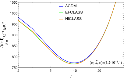
Figure 1: Left: The low-l multipoles of the TT CMB spectrum for a flat universe with $\Omega_{m,0}=0.3$, $n_{s}=1$, $A_{s}=2.3\cdot 10^{-9}$, $h=0.7$ and $(\tilde{c_{0}},\tilde{J_{c}},n)=(1,2\cdot 10^{-3},1)$. The values of values for $\tilde{J}_{c}$ were chosen so as to highlight the differences of these models with respect to GR. Our EFCLASS code is denoted by the green line, hi_CLASS by the orange line and for reference the $\Lambda$CDM with a blue line. Right: The percent difference of our code with hi_CLASS as a reference. As can be seen, our simple modification achieves roughly $\sim 0.1\%$ accuracy across all multipoles.

Finally we present our implementation of the effective fluid approach in the CLASS code Blas et al. (2011), which we call EFCLASS. The only changes we made in the code is in the perturbations.c file where we included the proper perturbations for the effective DE fluid given by Eqs. (6) and (8). We found that the most straight-forward and least error-prone way to make these changes is to modify the $\Lambda$CDM model equations in the aforementioned part of the code, as in the case of the perturbations, $\Lambda$CDM has none so we can just add the appropriate new terms given by Eqs. (6) and (8). We found that the best place to implement the modifications were in the perturb_einstein routine of CLASS, which solves the Einstein equations in the conformal Newtonian gauge given by Eqs. (6) and (8). Then, it is simple to just add in the right-hand-side of the aforementioned equations our expressions for the effective fluid DE velocity and anisotropic stress, which for the HDES model is zero.

Our analytic approach has several advantages: First, given that most viable $f(R)$ models and our HDES model can be written as small perturbations around $\Lambda$CDM model, it is always possible to derive extremely accurate expressions for the background, as was shown in Ref. Basilakos et al. (2013). Second, regarding the perturbations our improved subhorizon approximation gives much more accurate results compared to codes that are based on the default subhorizon approximation. Also, the accuracy is comparable to codes that treat the perturbations exactly by numerically solving the relevant equations. However, our approach has a much smaller overhead in terms of new lines of code and as a result is more straight-forward and less error-prone.

IV Conclusion

Given the plethora of modified gravity and dark energy theories where each model has its own structure, equations and parameters it is very difficult to analyse all of them at a technical level in an Einstein Boltzmann solver code. In this paper we have presented the effective fluid approach which allows to map any modified gravity model as an effective dark energy fluid and then we show how to implement it in the Boltzmann solver code CLASS in a simple and straightforward way finding competitive results in a much simpler and less error-prone approach in including the effects of modified gravity models. This method has also the advantage that only three variables are needed to compute to describe the fluid, i.e the equation of state $w(a)$ at the background level and the sound speed $c_{s}^{2}(a,k)$ and the anisotropic stress $\pi(a,k)$ at the linear perturbation.

In this paper we discussed in detail the effective fluid approach and perturbation theory in the context of $f(R)$ theories. We presented several new results, in particular regarding the effective DE fluid components of the energy momentum tensor, the effective velocity of the fluid $V_{DE}$ given by Eq. (26), the effective pressure and anisotropic stress by Eqs. (II.2) and (27). We then presented a family of designer Horndeski models, i.e. models that have a background exactly equal to that of the CDM model but perturbations given by the Horndeski theory. We implemented the parameterized version for the DE effective fluid of our $w_{DE}=-1$ designer Horndeski HDES model in the public code CLASS, which we call EFCLASS, by following the straightforward implementation explained with the $f(R)$ model.

For the sake of comparison and in order to check the validity of our effective fluid approach, we compared results from our code EFCLASS with the public code hi$\_$CLASS, which solves numerically the full perturbation equations. In Fig. 1 we show the CMB angular power spectrum computed with both codes and as can be seen in the right panel of Fig. 1, the agreement is remarkable and on average on the order of $\sim 0.1\%$. Since the hi$\_$CLASS code does not utilize neither the subhorizon nor the quasistatic approximation, but our EFCLASS does it, we conclude our effective fluid approach is quite accurate and powerful. Furthermore, the main advantage of our method is that while hi_CLASS requires significant and non-trivial modifications, our EFCLASS code practically only requires the implementation of Eq. 40, which is trivial.

Numerical Analysis Files: The numerical codes for the modifications to the CLASS code, dubbed EFCLASS, can be found at https://members.ift.uam-csic.es/savvas.nesseris/efclass.html, but also at the GitHub repositories https://github.com/wilmarcardonac/EFCLASS and https://github.com/RubenArjona/EFCLASS.

References

- Aghanim et al. (2018) N. Aghanim et al. (Planck) (2018), eprint 1807.06209.
- Abbott et al. (2018) T. M. C. Abbott et al. (DES), Phys. Rev. D98, 043526 (2018), eprint 1708.01530.
- Riess (2019) A. G. Riess, Nature Rev. Phys. 2, 10 (2019), eprint 2001.03624.
- Hinshaw et al. (2013) G. Hinshaw et al. (WMAP), Astrophys. J. Suppl. 208, 19 (2013), eprint 1212.5226.
- Arjona and Nesseris (2019) R. Arjona and S. Nesseris (2019), eprint 1910.01529.
- Arjona and Nesseris (2020) R. Arjona and S. Nesseris (2020), eprint 2001.11420.
- Bertone and Hooper (2018) G. Bertone and D. Hooper, Rev. Mod. Phys. 90, 045002 (2018), eprint 1605.04909.
- Weinberg (1989) S. Weinberg, Rev. Mod. Phys. 61, 1 (1989), [,569(1988)].
- Carroll (2001) S. M. Carroll, Living Rev. Rel. 4, 1 (2001), eprint astro-ph/0004075.
- Verde et al. (2019) L. Verde, T. Treu, and A. G. Riess, in Nature Astronomy 2019 (2019), eprint 1907.10625.
- Copeland et al. (2006) E. J. Copeland, M. Sami, and S. Tsujikawa, Int. J. Mod. Phys. D15, 1753 (2006), eprint hep-th/0603057.
- Ratra and Peebles (1988) B. Ratra and P. J. E. Peebles, Phys. Rev. D37, 3406 (1988).
- Clifton et al. (2012) T. Clifton, P. G. Ferreira, A. Padilla, and C. Skordis, Phys. Rept. 513, 1 (2012), eprint 1106.2476.
- Nadkarni-Ghosh and Refregier (2017) S. Nadkarni-Ghosh and A. Refregier, Mon. Not. Roy. Astron. Soc. 471, 2391 (2017), eprint 1612.06697.
- Kodama and Sasaki (1984) H. Kodama and M. Sasaki, Progress of Theoretical Physics Supplement 78, 1 (1984).
- Sugiyama (1989) N. Sugiyama, Progress of Theoretical Physics 81, 1021 (1989).
- Ma and Bertschinger (1995) C.-P. Ma and E. Bertschinger, Astrophys. J. 455, 7 (1995), eprint astro-ph/9506072.
- Lewis et al. (2000) A. Lewis, A. Challinor, and A. Lasenby, Astrophys. J. 538, 473 (2000), eprint astro-ph/9911177.
- Lesgourgues (2011) J. Lesgourgues (2011), eprint 1104.2932.
- Alonso et al. (2017) D. Alonso, E. Bellini, P. G. Ferreira, and M. Zumalacárregui, Phys. Rev. D95, 063502 (2017), eprint 1610.09290.
- Arjona et al. (2019a) R. Arjona, W. Cardona, and S. Nesseris, Phys. Rev. D99, 043516 (2019a), eprint 1811.02469.
- Arjona et al. (2019b) R. Arjona, W. Cardona, and S. Nesseris, Phys. Rev. D100, 063526 (2019b), eprint 1904.06294.
- Kunz (2012) M. Kunz, Comptes Rendus Physique 13, 539 (2012), eprint 1204.5482.
- Huterer (2010) D. Huterer, Gen. Rel. Grav. 42, 2177 (2010), eprint 1001.1758.
- Cardona et al. (2019) W. Cardona, R. Arjona, and S. Nesseris (2019), eprint 1907.10130.
- Multamaki and Vilja (2006) T. Multamaki and I. Vilja, Phys. Rev. D73, 024018 (2006), eprint astro-ph/0506692.
- de la Cruz-Dombriz and Dobado (2006) A. de la Cruz-Dombriz and A. Dobado, Phys. Rev. D74, 087501 (2006), eprint gr-qc/0607118.
- Pogosian and Silvestri (2008) L. Pogosian and A. Silvestri, Phys. Rev. D77, 023503 (2008), [Erratum: Phys. Rev.D81,049901(2010)], eprint 0709.0296.
- Nesseris (2013) S. Nesseris, Phys. Rev. D88, 123003 (2013), eprint 1309.1055.
- Nesseris and Shafieloo (2010) S. Nesseris and A. Shafieloo, Mon. Not. Roy. Astron. Soc. 408, 1879 (2010), eprint 1004.0960.
- Nesseris and Garcia-Bellido (2012) S. Nesseris and J. Garcia-Bellido, JCAP 1211, 033 (2012), eprint 1205.0364.
- Tsujikawa (2007) S. Tsujikawa, Phys. Rev. D76, 023514 (2007), eprint 0705.1032.
- Horndeski (1974) G. W. Horndeski, Int. J. Theor. Phys. 10, 363 (1974).
- Baker et al. (2013) T. Baker, P. G. Ferreira, and C. Skordis, Phys. Rev. D87, 024015 (2013), eprint 1209.2117.
- Creminelli and Vernizzi (2017) P. Creminelli and F. Vernizzi, Phys. Rev. Lett. 119, 251302 (2017), eprint 1710.05877.
- Sakstein and Jain (2017) J. Sakstein and B. Jain, Phys. Rev. Lett. 119, 251303 (2017), eprint 1710.05893.
- Ezquiaga and Zumalacarregui (2017) J. M. Ezquiaga and M. Zumalacarregui, Phys. Rev. Lett. 119, 251304 (2017), eprint 1710.05901.
- Baker et al. (2017) T. Baker, E. Bellini, P. G. Ferreira, M. Lagos, J. Noller, and I. Sawicki, Phys. Rev. Lett. 119, 251301 (2017), eprint 1710.06394.
- Amendola et al. (2018) L. Amendola, M. Kunz, I. D. Saltas, and I. Sawicki, Phys. Rev. Lett. 120, 131101 (2018), eprint 1711.04825.
- Crisostomi and Koyama (2018) M. Crisostomi and K. Koyama, Phys. Rev. D97, 084004 (2018), eprint 1712.06556.
- Frusciante et al. (2018) N. Frusciante, S. Peirone, S. Casas, and N. A. Lima (2018), eprint 1810.10521.
- Kase and Tsujikawa (2018) R. Kase and S. Tsujikawa (2018), eprint 1809.08735.
- McManus et al. (2016) R. McManus, L. Lombriser, and J. Peï¿œarrubia, JCAP 1611, 006 (2016), eprint 1606.03282.
- Lombriser and Taylor (2016) L. Lombriser and A. Taylor, JCAP 1603, 031 (2016), eprint 1509.08458.
- Copeland et al. (2019) E. J. Copeland, M. Kopp, A. Padilla, P. M. Saffin, and C. Skordis, Phys. Rev. Lett. 122, 061301 (2019), eprint 1810.08239.
- Noller and Nicola (2018) J. Noller and A. Nicola (2018), eprint 1811.03082.
- de Rham and Melville (2018) C. de Rham and S. Melville, Phys. Rev. Lett. 121, 221101 (2018), eprint 1806.09417.
- Abbott et al. (2017) B. P. Abbott et al. (Virgo, LIGO Scientific), Phys. Rev. Lett. 119, 141101 (2017), eprint 1709.09660.
- Sotiriou and Faraoni (2010) T. P. Sotiriou and V. Faraoni, Rev. Mod. Phys. 82, 451 (2010), eprint 0805.1726.
- De Felice and Tsujikawa (2010) A. De Felice and S. Tsujikawa, Living Rev. Rel. 13, 3 (2010), eprint 1002.4928.
- Nojiri et al. (2017) S. Nojiri, S. D. Odintsov, and V. K. Oikonomou, Phys. Rept. 692, 1 (2017), eprint 1705.11098.
- Nojiri and Odintsov (2011) S. Nojiri and S. D. Odintsov, Phys. Rept. 505, 59 (2011), eprint 1011.0544.
- Deffayet et al. (2010) C. Deffayet, O. Pujolas, I. Sawicki, and A. Vikman, JCAP 1010, 026 (2010), eprint 1008.0048.
- Kunz and Sapone (2007) M. Kunz and D. Sapone, Phys. Rev. Lett. 98, 121301 (2007), eprint astro-ph/0612452.
- Pogosian et al. (2010) L. Pogosian, A. Silvestri, K. Koyama, and G.-B. Zhao, Phys. Rev. D81, 104023 (2010), eprint 1002.2382.
- Capozziello et al. (2006a) S. Capozziello, S. Nojiri, and S. D. Odintsov, Phys. Lett. B634, 93 (2006a), eprint hep-th/0512118.
- Capozziello et al. (2006b) S. Capozziello, S. Nojiri, S. D. Odintsov, and A. Troisi, Phys. Lett. B639, 135 (2006b), eprint astro-ph/0604431.
- Capozziello et al. (2019) S. Capozziello, C. A. Mantica, and L. G. Molinari, Int. J. Geom. Meth. Mod. Phys. 16, 1950008 (2019), eprint 1810.03204.
- Sapone and Kunz (2009) D. Sapone and M. Kunz, Phys. Rev. D80, 083519 (2009), eprint 0909.0007.
- Chiba (2003) T. Chiba, Phys. Lett. B575, 1 (2003), eprint astro-ph/0307338.
- Brans and Dicke (1961) C. Brans and R. H. Dicke, Phys. Rev. 124, 925 (1961), [,142(1961)].
- Quiros (2019) I. Quiros (2019), eprint 1901.08690.
- Kimura and Yamamoto (2011) R. Kimura and K. Yamamoto, JCAP 1104, 025 (2011), eprint 1011.2006.
- Blas et al. (2011) D. Blas, J. Lesgourgues, and T. Tram, JCAP 1107, 034 (2011), eprint 1104.2933.
- Basilakos et al. (2013) S. Basilakos, S. Nesseris, and L. Perivolaropoulos, Phys. Rev. D87, 123529 (2013), eprint 1302.6051.