QCD beyond diagrams

Abstract

QCD, the theory of the strong interactions, involves quarks interacting with non-Abelian gluon fields. This theory has many features that are difficult to impossible to see in conventional diagrammatic perturbation theory. This includes quark confinement, mass generation, and chiral symmetry breaking. This paper is a colloquium level overview of the framework for understanding how these effects come about.

I Introduction

The standard model of particle physics combines electrodynamics, the weak interactions responsible for beta decay, and the strong interactions of nuclear physics. The strong interaction sector is based on quarks interacting via the exchange of non-Abelian gluon fields, and is referred to as “QCD” or “quantum chromodynamics.” It is in some sense the best defined part of the standard model. Unlike electrodynamics, the behavior of QCD is controlled at short distances by the phenomenon of “asymptotic freedom.” While electrodynamics may have numerous successes, it remains unclear if it is well defined on its own. The weak interactions have additional issues associated with the absence of a rigorous non-perturbative scheme for incorporating parity violation.

Most of our quantitative understanding of quantum field theory comes by way of perturbative expansions. However, QCD has several features that are difficult to impossible to understand in terms of Feynman diagrams. First is confinement; quarks do not propagate as free particles, but always appear in color singlet bound states. Second, the theory generates its own mass scale; even if the quarks are massless, the proton is not. Third is the presence of chiral symmetry breaking, responsible for the pion being much lighter than the rho, although both are made of the same quarks. And finally, the theory depends on a hidden parameter, usually called “Theta.” Different values of Theta represent physically inequivalent theories, despite having identical perturbative expansions. The framework for investigating how these phenomena come about in QCD is the subject of this paper. For those interested in more details, see the book From Quarks to Pions Creutz (2018).

II Path integrals

Our discussion revolves around the Feynman path integral formulation of quantum mechanics. Feynman’s classic 1948 article demonstrated a remarkable equivalence between a quantum mechanical system and a statistical mechanics problem in one more dimension Feynman (1948). Consider a particle moving in some potential $V(x)$ and an action function for an arbitrary path $x(t)$ between $t=0$ and $t=\beta$

$$S=\int_{0}^{\beta}dt\ \dot{x}^{2}/2+V(x)$$ (1)

Feynman showed that by integrating over all possible paths, there is an equivalence to the quantum mechanics of a unit mass particle moving in the potential $V$ with Hamiltonian

$$H=\hat{p}^{2}/2+V(\hat{x})$$ (2)

where $\hat{x}$ and $\hat{p}$ are quantum mechanical operators satisfying the canonical commutation relation

$$[\hat{p},\hat{x}]\equiv\hat{p}\hat{x}-\hat{x}\hat{p}=i.$$ (3)

Formally we have

$$\int(dx(t))\ e^{-S(x(t))}\qquad\propto\qquad{\rm Tr}\ e^{-\beta H}$$ (4)

where the trace is over the quantum mechanical Hilbert space. To define what is meant by integrating over paths, Feynman introduced a discretization of time in steps of size $a$ and then integrated over the position on each time slice, as sketched in Fig. 1. The path integral is defined in a limit $a\rightarrow 0$.

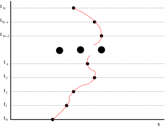
Figure 1: Dividing time into slices to define the path integral.

This process proceeds similarly for field theories, with a $D$ dimensional quantum field theory related to a $D+1$ dimensional statistical mechanics problem. In field theory the “paths” are usually referred to as “configurations.” This approach is the heart of the Monte Carlo approach to lattice gauge theory.

In this picture, a path looks much like a wiggling string or worm. As the time spacing becomes small, this worm becomes increasingly wiggly. Indeed, in the limit $a\rightarrow 0$ the typical paths are not differentiable in the sense that

$$\langle\dot{x}^{2}\rangle=\left\langle\left({x_{i+1}-x_{i}\over a}\right)^{2}\right\rangle\propto{1\over a}\rightarrow\infty.$$ (5)

This roughness extends to the field theory case, wherein the typical configurations are also non-differentiable. This raises interesting ambiguities to which we return in Section X.

III Perturbation theory

At this point traditional treatments of quantum field theory turn to perturbation theory. Divide the action into two parts

$$S=S_{0}+gS_{I}$$ (6)

where $S_{0}$ describes a solvable theory of free particles and $S_{I}$ couples the fields together. Expanding the path integral in the coupling $g$ gives the usual Feynman diagrams wherein free propagators are coupled by interaction vertices. But, for our purposes, it is important to realize that the path integral approach is much more general.

For the electro-weak part of the standard model, the basic coupling $\alpha={g^{2}\over 4\pi}\sim 1/137$ is a small number, and perturbation theory works well for all practical purposes. However Dyson provided a simple argument that perturbation theory cannot converge Dyson (1952). He argued that if it did, then one could analytically continue $e\rightarrow ie$ and we would have a theory where like charges attract instead of repel. In this case one could produce separate regions of charge large enough to bind additional electrons by more than their rest mass. One could use this situation to create a perpetual motion machine by creating electron positron pairs and sending them to the respective charged regions. This is sketched in Fig. 2. The vacuum of such a theory is unstable.

Figure 2: If like charges attracted, one could create an unstable situation by creating two large regions of opposite charge and tossing particle-antiparticle pairs into them.

The problems with perturbation theory are particularly acute with QCD, the theory of quarks and gluons. If the coupling vanishes, $g=0$, the physical propagating fields are quarks and massless gluons. However as soon as $g\neq 0$ we have a theory where the physical particles are protons and pions. This is a qualitatively different spectrum. The gluon electric fields between quark charges change from a Coulombic spread into a flux tube giving a linear potential, as sketched in Fig. 3. To understand these qualitative changes, one must go beyond perturbation theory.

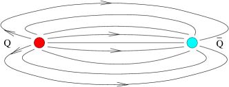
Figure 3: The gluon electric field between quark pairs becomes concentrated into a tube of flux with a net energy per unit length. The tension in this string is roughly 14 tons.

IV Divergences and renormalization

As is well known, relativistic quantum field theory is replete with divergences that require renormalization. One must introduce a cutoff, and then remove it by a limiting procedure. The basic idea is to fix a few physical observables and adjust the bare couplings and masses in such a way that the physics remains finite as the cutoff is removed. In the process the bare charges and masses absorb the divergences by either going to infinity or zero.

Historically most regulators used in practice, such as Pauli-Villars or dimensional, are based on perturbation theory. One starts to calculate and on finding a divergent diagram inserts the cutoff. But QCD requires a non-perturbative regulator. This is where lattice gauge theory comes in, with the lattice spacing $a$ being a cutoff. In terms of the world lines a quark might take, they are replaced by single steps on the lattice, as sketched in Fig. 4. Most lattice formulations are based on Wilson’s Wilson (1974) elegant picture of quarks hopping between sites while picking up non-Abelian phases on the bonds. We return to this in Section VII.

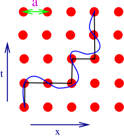
Figure 4: On the lattice a world line of any particle is replaced by a sequence of discrete hops. The size of these hops represents an ultraviolet cutoff and should be taken to zero for the continuum limit.

As a simple example of how renormalization might theoretically proceed, consider taking the proton mass as the physical observable. This is expected to remain finite, even if the quark masses vanish. Ignoring quark masses for the moment, the proton mass is a function of the lattice spacing $a$ and the coupling $g$. We want to vary the coupling for the continuum limit so the proton mass is constant. For this we have

$$a{d\over da}m_{p}(a,g)=0=\left({\partial\over\partial g}m_{p}\right)\left(a{dg\over da}\right)+a{\partial\over\partial a}m_{p}.$$ (7)

Since the only dimensional input is the lattice spacing, dimensional analysis tells us

$$a{\partial\over\partial a}m_{p}=-m_{p}.$$ (8)

Putting this together, we conclude

$$a{dg\over da}\equiv\beta(g)={m_{p}\over{\partial\over\partial g}m_{p}}.$$ (9)

This totally non-perturbative definition shows formally how $g$ should depend on $a$ for the physical limit.

V Asymptotic freedom

While shirking perturbation theory to this point, a remarkable feature of the function $\beta(g)$ is that it does itself have an expansion in $g$, and this expansion gives non-perturbative information on how to take the continuum limit. Gross, Wilczek, and Politzer in their Nobel Prize winning papers showed Gross and Wilczek (1973); Politzer (1973)

$$\beta(g)=\beta_{0}g^{3}+\beta_{1}g^{5}+O(g^{7})$$ (10)

where

$$\beta_{0}={1\over 16\pi^{2}}(11-2N_{f}/3)$$ (11)

and $N_{f}$ is the number of distinct quark “flavors” under consideration Gross and Wilczek (1973); Politzer (1973). A year later Caswell and JonesCaswell (1974); Jones (1974) calculated

$$\beta_{1}=\left({1\over 16\pi^{2}}\right)^{2}(102-22N_{f}/3).$$ (12)

A remarkable feature of this expansion is that $\beta_{0}$ and $\beta_{1}$ are independent of the details of the regularization scheme, although higher terms are not. This means that this result is immediately applicable to the lattice as well.

The differential equation obtained by combining Eqs. (9) and (10)

$$a{dg\over da}=\beta_{0}g^{3}+\beta_{1}g^{5}+O(g^{7})$$ (13)

is easy to solve, giving

$$a={1\over\Lambda}\ g^{-\beta_{1}/\beta_{0}^{2}}\ \exp\left({-1\over 2\beta_{0}g^{2}}\right)\ (1+O(g^{2}))$$ (14)

where $\Lambda$ is an integration constant. Note the factor of $\exp\left({-1\over 2\beta_{0}g^{2}}\right)$ has an essential singularity and cannot be expanded in a power series in $g$. This equation also shows that taking the lattice spacing to zero requires $g$ to go to zero. This is what is called “asymptotic freedom.”

The integration constant $\Lambda$ has dimensions of mass. While the classical theory with massless quarks contains no dimensional scale, renormalization forces us to bring one in. All particle masses, including the proton, are proportional to $\Lambda$

$$m_{p}\propto\Lambda\propto{1\over a}\ g^{-\beta_{1}/\beta_{0}^{2}}\ \exp\left({-1\over 2\beta_{0}g^{2}}\right)$$ (15)

again showing non-perturbative behavior! The idea that renormalization can eliminate a dimensionless coupling $g$ while generating an overall mass scale has been given the marvelous name “dimensional transmutation” Coleman and Weinberg (1973).

VI Mass renormalization

So far we have ignored the masses of the quarks. These also need to be renormalized, requiring additional physical things to be fixed for the continuum limit. That brings in more integration constants. We’ll be brief here and only note that the bare mass $m$ of any quark flavor should satisfy

$$a{dm\over da}=m\gamma(g)=m(\gamma_{0}g^{2}+\dots)+\hbox{ non perturbative}$$ (16)

where $\gamma_{0}={8\over(4\pi)^{2}}$ Georgi and Politzer (1976). The “non-perturbative” expression in the above equation allows terms that fall faster than any power of $g$ and will play a role in later discussion. As before, this equation is easily integrated

$$m=M\ g^{\gamma_{0}/\beta_{0}}\ (1+O(g^{2}))$$ (17)

where $M$ is another integration constant. There is one such $M_{i}$ corresponding to each quark species $i$. Note that since $g$ goes to zero for the continuum limit, so do the bare quark masses $m_{i}$. The full continuum requires taking both the bare $g$ and $m$ together, as sketched in Fig 5.

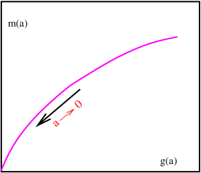
Figure 5: For the continuum limit, both the bare coupling and quark masses flow towards vanishing values.

The continuum theory depends only on the dimensional integration constants $M_{i}$ and $\Lambda$. Once these are known, all physical results are in principle determined. While they depend on the physical quantities held fixed for renormalization, their specific values depend on the details of the regulator. As will be discussed in Section X, they can mix together depending on the details of the scheme. The physical observables being held fixed, such as the proton and pseudoscalar masses, are all that the theory ultimately depends on.

VII The lattice

The primary role of lattice gauge theory is as a non-perturbative regulator. It provides a minimum wavelength through the lattice spacing $a$, i.e. a maximum momentum of $\pi/a$. Avoiding the convergence difficulties of perturbation theory, the lattice provides a route towards a rigorous definition of a quantum field theory as a limiting process.

As formulated by Wilson, the lattice cutoff remains true to many of the underlying concepts of a gauge theory. In particular a gauge theory is a theory with a local symmetry. With the Wilson action being formulated in terms of products of group elements around closed loops, this symmetry remains exact even with the regulator in place.

The concept of gauge fields representing path dependent phases leads directly to the conventional lattice formulation. We approximate a general quark world line by a set of hoppings lying along lattice bonds, as sketched earlier in Fig. 4. The gauge field corresponds to $SU(3)$ phases acquired along these hoppings. Thus the gauge fields are a set, $\{U\}$, of group matrices, one element associated with each nearest neighbor bond of the four-dimensional space-time lattice.

Motivated by the electromagnetic flux being the generalized curl of the vector potential, we identify the flux through an elementary square, or “plaquette,” on the lattice with the phase factor obtained on running around that plaquette; see Fig. 6. Spatial plaquettes represent the “magnetic” effects and plaquettes with one time-like side give the “electric” fields. This motivates the conventional “action” used for the gauge fields as a sum over all elementary squares of the lattice. Around each square we multiply the phases and take the real part of the trace

$$S_{g}=\sum_{p}{\rm Re\ Tr}\prod_{l\in p}U_{l}\sim\int d^{4}x\ E^{2}+B^{2}.$$ (18)

Here the fundamental squares are denoted $p$ and the links $l$. As we are dealing with non-commuting matrices, the product around the square is meant to be ordered, while, because of the trace, the starting point of this ordering drops out.

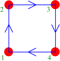
Figure 6: Analogous to Stoke’s law, the flux through an elementary square of the lattice is found from the product of gauge matrices around that square. The dynamics is determined by adding the real part of the trace of this product over all elementary squares.

For the quantum theory we turn to the path integral. To construct this, exponentiate the action and integrate over all dynamical variables

$$Z=\int(dU)e^{-\beta S},$$ (19)

where the parameter $\beta$ controls the bare coupling. This converts the three space dimensional quantum field theory of gluons into a classical statistical mechanical system in four space-time dimensions.

The formulation is conventionally taken in Euclidean four-dimensional space. In effect this replaces the time evolution operator $e^{-iHt}$ by $e^{-Ht}$. Then the path integral involves positive weights, and can be studied by standard Monte Carlo methods. This approach currently dominates lattice gauge research. The simulations have had numerous successes, from demonstrating confinement Creutz (1980) to reproducing the hadronic spectrum Durr et al. (2011).

VIII Pions as pseudo-Goldstone bosons

Much older a tool than the lattice, ideas based on chiral symmetry have historically provided considerable insight into how the strong interactions work. In particular, chirality is crucial to our understanding of why the pion is so much lighter than the rho, despite being made of the same quarks.

The classical Lagrangian for QCD couples left and right handed quark fields only through mass terms. If we project out the two helicity states of a quark field by defining

$$\psi_{L}={1+\gamma_{5}\over 2}\psi\qquad\psi_{R}={1-\gamma_{5}\over 2}\psi$$ (20)

then the classical kinetic term for the quarks separates

$$i\overline{\psi}D\psi=i\overline{\psi}_{L}D\psi_{L}+i\overline{\psi}_{R}D\psi_{R}.$$ (21)

On the other hand, the mass term directly mixes the two chiralities

$$m\overline{\psi}\psi=m\overline{\psi}_{R}\psi_{L}+m\overline{\psi}_{L}\psi_{R}.$$ (22)

Thus naively the massless theory appears to have independent conserved quantities, one associated with each handedness. After confinement, it is generally understood that the axial chiral symmetry is spontaneously broken via the scalar field $\sigma\propto\overline{\psi}\psi$ acquiring a vacuum expectation value. As with the mass term, this field mixes chiralities. This expectation value is not invariant under the axial chiral symmetry. Although chiral symmetry is broken, parity is not; it is only the independence of the left and right quark fields that the vacuum does not respect.

For $N_{f}$ massless flavors, there is classically an independent $U(N_{f})$ symmetry associated with each chirality, giving what is often written in terms of axial and vector fields as an $U(N_{f})_{V}\otimes U(N_{f})_{A}$ symmetry. As we will see in the following section, this full symmetry does not survive quantization, being broken to a $SU(N_{f})_{V}\otimes SU(N_{f})_{A}\otimes U(1)_{B}$, where the $U(1)_{B}$ represents the symmetry of baryon number conservation. The only surviving axial symmetries of the massless quantum theory are non-singlet under flavor symmetry.

We work here with composite scalar and pseudo-scalar fields

$$\matrix{\sigma&\sim&\overline{\psi}\psi\cr\pi_{\alpha}&\sim&i\overline{\psi}\lambda_{\alpha}\gamma_{5}\psi\cr\eta^{\prime}&\sim&i\overline{\psi}\gamma_{5}\psi.\cr}$$ (23)

Here the $\lambda_{\alpha}$ are the generators for the flavor group $SU(N_{f})$. They are generalizations of the usual Gell-Mann matrices from $SU(3)$; however, now we are concerned with the flavor group, not the internal symmetry group related to confinement. As mentioned earlier, we must assume that some sort of regulator, perhaps a lattice, is in place to define these products of fields at the same point. Indeed, most of the quantities mentioned in this section are formally divergent, although we concentrate on those aspects that survive the continuum limit.

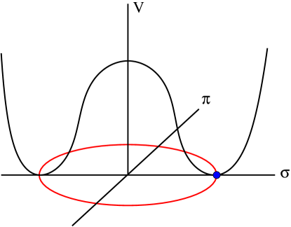
Figure 7: The flavor non-singlet pseudo-scalar mesons are Goldstone bosons corresponding to flat directions in the effective potential. This shape is sometimes referred to as a “Mexican hat” or “a wine-bottle bottom” potential.

The conventional picture of spontaneous chiral symmetry breaking in the limit of massless quarks assumes that the vacuum acquires a quark condensate with

$$\langle\overline{\psi}\psi\rangle=\langle\sigma\rangle=v\neq 0.$$ (24)

Extending the effective potential to a function of multiple non-singlet pseudo-scalar fields gives the standard picture of Goldstone bosons. These are massless when the quark mass vanishes, corresponding to $N_{f}^{2}-1$ “flat” directions for the potential. One such direction is sketched schematically in Fig. 7. For the two flavor case, these rotations represent a symmetry mixing the sigma field with any of the pions

$$\matrix{\sigma\rightarrow\phantom{+}\sigma\cos(\phi)+\pi^{\alpha}\sin(\phi)\cr\pi^{\alpha}\rightarrow-\sigma\sin(\phi)+\pi^{\alpha}\cos(\phi).\cr}$$ (25)

Pions are waves propagating through the non-vanishing sigma condensate with oscillations in a direction “transverse” to the sigma expectation. They are massless because there is no restoring force in that direction.

If we now introduce a small mass for the quarks, this will effectively tilt the potential $V(\sigma)\rightarrow V(\sigma)-m\sigma$. This selects one minimum as the true vacuum. The tilting of the potential breaks the global symmetry and gives the Goldstone bosons a small mass proportional to the square root of the quark mass, as sketched in Fig. 8. With non-degenerate quarks, it is the average quark mass that gives the pseudoscalar mass; i.e. for the charged pion we have

$$M_{\pi^{+}}^{2}\propto{m_{u}+m_{d}\over 2}\Lambda.$$ (26)

The standard chiral Lagrangian approach is a simultaneous expansion in the masses and momenta of these light particles.

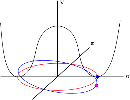
Figure 8: A small quark mass term tilts the effective potential, selecting one direction for the true vacuum and giving the Goldstone bosons a mass proportional to the square root of the quark mass.

IX Topology and chiral symmetry

So far we have concentrated on aspects of the quantum theory. But non-perturbative phenomena also play a role in the classical theory Yang and Mills (1954). With non-Abelian gluon fields, a boundary condition such as the vanishing of the field $F_{\mu\nu}$ at spatial infinity does not require the gauge potential $A_{\mu}\rightarrow 0$, but only that the potential be a gauge transformation of zero field, i.e.

$$A_{\mu}\longrightarrow-{1\over g^{2}}h^{\dagger}\partial_{\mu}h$$ (27)

where $h$ is a group valued function of space. For our four dimensional world, the space at infinity is sphere $S_{3}$ and the function $h(x)$ can wrap non-trivially about this sphere. The space of smooth gauge fields separates into sectors labeled by this winding, which can be determined directly from the gauge fields

$${g^{2}\over 16\pi^{2}}\int d^{4}x{\rm Tr}F\tilde{F}=\nu$$ (28)

where the index $\nu$ is an integer. The path integral should sum over all such sectors. Of course, as mentioned earlier, the typical gauge configuration is not smooth; indeed, it is not differentiable in the continuum limit. This introduces a small ambiguity in defining the winding; we will return to this briefly in Section X.

These topological issues become particularly relevant upon introducing fermion fields, i.e. the quarks. Whenever $\nu\neq 0$ the Dirac operator has zero modes satisfying

$$D\psi(x)=\gamma_{\mu}(\partial_{\mu}+igA_{\mu})\psi(x)=0.$$ (29)

Furthermore these modes are chiral

$$\gamma_{5}\psi(x)=\pm\psi(x).$$ (30)

The basic index theorem relates the number of such modes to the index in Eq. (28)

$$\nu=n_{+}-n_{-}$$ (31)

where $n_{+}$ and $n_{-}$ are the number of positive or negative chiral zero modes, respectively.

The importance of the zero modes was nicely interpreted in Fujikawa (1979). Configurations with non-trivial winding exist and must be included in the path integral. On these formally

$${\rm Tr}\gamma_{5}\equiv\sum_{i}\langle\psi_{i}\gamma_{5}\psi_{i}\rangle=\nu\neq 0.$$ (32)

where the sum is over a complete set of modes of the Dirac operator. All other than the zero modes occur either in chiral-conjugate pairs or “above the cutoff” and don’t contribute to the sum. On such configurations the naive chiral transformation

$$\psi\rightarrow e^{i\gamma_{5}\theta}\psi$$ (33)

is not a symmetry. Instead it changes the fermion measure in the path integral

$$d\psi\rightarrow|e^{i\gamma_{5}\Theta}|\ d\psi=e^{i\nu\Theta}\ d\psi.$$ (34)

If we try to make the change of variables in Eq. (33), topology inserts a factor of $e^{i\nu\Theta}$ into the path integral. This gives rise to a new and inequivalent theory. This breaking of the naive chiral symmetry is at the heart of why the $\eta^{\prime}$ particle is heavier than the pseudo-Goldstone mesons and its mass is not directly proportional to the quark masses. Indeed, $\Theta$ is a hidden non-perturbative parameter for QCD. For each value of $\Theta$, the perturbative expansion is identical! Perturbation theory alone does not fully define the theory.

Note that the special case $\Theta=\pi$ reverses the sign of the quark mass term

$$m\overline{\psi}\psi\rightarrow-m\overline{\psi}\psi.$$ (35)

This means that three flavor QCD with negative masses is a different theory, i.e QCD at $\Theta=\pi$. This is in strong contrast to perturbation theory, wherein the sign of a fermion mass is merely a convention.

The possibility of $\Theta\neq 0$ raises an as yet unresolved puzzle. In this case CP symmetry is violated. As no CP violation has been observed in the strong interactions, experimentally $\Theta$ must be very small. Since CP violation is seen in the weak interactions, why are the strong interactions different?

X Confinement and quark masses

Quarks are confined in hadrons. What does their mass mean? For a physical particle, such as the proton, the mass follows from how it travels over long distances. We measure a particle mass seeing how its energy and velocity are related

$$E=mc^{2}+{1\over 2}mv^{2}+O(mv^{4}/c^{2}).$$ (36)

We can’t use this relation for quarks since they don’t propagate alone. Indeed the quark propagator is a gauge and scheme dependent quantity.

The renormalization group integration constant $M$ would seem to be a natural candidate for a renormalized quark mass

$$m=M\ g^{\gamma_{0}/\beta_{0}}(1+O(g^{2}))+\hbox{non-perturbative}.$$ (37)

But some time ago ’t Hooft ’t Hooft (1976) showed that the “non-perturbative” effects will mix the various $M_{i}$ and $\Lambda$ in non-trivial ways. With a lattice regulator, this mixing can depend on the details of the lattice regularization scheme.

Chiral symmetry provides one handle on this. With degenerate light quarks, we have light pseudoscalar bound states. In particular, massless quarks imply massless pions. For degenerate quarks, the concept of a vanishing quark mass, $m_{q}=0$, is well defined.

When the quarks are not degenerate, the situation is more complicated. Simple chiral perturbation theory indicates that the mass of a pseudoscalar is proportional to the average of its constituent masses, as in Eq. (26). Combining such relations with different particles gives estimates for quark mass ratios. For example

$${m_{u}\over m_{d}}\sim{2m_{\pi^{0}}^{2}-m_{\pi^{+}}^{2}+m_{K_{+}}^{2}-m_{K_{0}}^{2}\over m_{\pi^{+}}^{2}-m_{K_{+}}^{2}+m_{K_{0}}^{2}}\sim 0.55$$ (38)

suggests that the up quark has about half the down quark mass. This particular combination is chosen to reduce electromagnetic corrections Dashen (1969).

Eq. (38) must be understood in the context of several caveats. First, different meson combinations give slightly different values for this ratio due to the chiral expansion being only an approximation and higher order effects being ignored Kaplan and Manohar (1986). Second, when the quarks are not degenerate, mixing occurs between the various neutral pseudoscalar mesons. When the strange quark is included, near the chiral limit the mixing is primarily with the eta. This is incorporated into the generalization of Eq. (26)

$$m_{\pi_{0}}^{2}\propto\ {1\over 3}\bigg{(}m_{u}+m_{d}+m_{s}-\sqrt{m_{u}^{2}+m_{d}^{2}+m_{s}^{2}-m_{u}m_{d}-m_{u}m_{s}-m_{d}m_{s}}\bigg{)}.$$ (39)

This is not the whole story since further mixing occurs with the eta prime and pure gluonic states, particles that obtain the bulk of their mass independent of chiral symmetry. Concentrating on the lightest two flavors, isospin breaking starts out quadratic in up-down mass difference

$${M_{\pi_{0}}\over M_{\pi_{+}}}=1-O\left({(m_{d}-m_{u})^{2}\over m_{s}^{2}},{(m_{d}-m_{u})^{2}\over\Lambda^{2}}\right).$$ (40)

The low masses of the up and down quarks makes this splitting quite small for the physical pions, even though the up quark is only about half as heavy as the down. The scale for the correction involves the masses of the higher states. For the mixing with the eta the correction is contained in Eq. (39). For the eta prime and the glue states that scale is not determined directly by the quark masses but involves the scale $\Lambda$. One consequence is that holding quark mass ratios fixed during renormalization is only approximately equivalent to holding physical particle mass ratios constant.

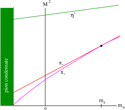
Figure 9: As the up quark mass decreases to negative values, the neutral pion mass can pass through zero, giving rise to a $\pi_{0}$ condensate.

Although isospin breaking is small in practice, it is interesting to consider what could happen if the light quark mass difference were larger. Note in particular that Eq. (26) indicates that a mass gap persists if only one quark, say the up quark, is massless when the other quarks have positive mass. Furthermore it appears that physics remains sensible even if the up quark has small negative mass. Remember, as mentioned earlier, in perturbation theory the sign of a fermion mass is a convention. This is not the case for QCD.

A particularly interesting situation occurs if the up quark mass is negative enough, i.e. $m_{u}=O(-m_{d})$. The neutral pion decreases in mass and eventually can pass through zero. This gives rise to a condensation of the $\pi_{0}$ field as sketched in Fig. 9. This CP violating condensate is referred to as the Dashen phase Dashen (1971).

The neutral pion also provides a simple example of how confinement entangles the quark masses. This particle is a bound state of left and right handed quarks and involves both up and down quark species. If we create the $\pi_{0}$ from up quarks, $i\overline{u}_{L}\gamma_{5}u_{R}$, and then destroy it using down quarks, $i\overline{d}_{L}\gamma_{5}d_{R}$, we have a spin flip process, as shown in Fig. 10. Unlike in perturbation theory, this is not suppressed at small light-quark masses. It is due to topology through what is called the “’t Hooft vertex” ’t Hooft (1976).

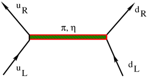
Figure 10: A spin flip process involving both the up and down quarks occurs on exchanging pseudoscalar mesons. The $\pi$ and $\eta$ contributions cannot cancel since they are non-degenerate.

We see that the naive result that left and right handed quark fields decouple at $m=0$ fails non-perturbatively. Furthermore, this induces a mass mixing for different quark species. If we turn on a small down quark mass in Fig. 10 and close the down quark lines in a loop, we arrive at Fig. 11. This shows that a non-vanishing down quark mass can generate an effective mass for the up quark, even if it started off massless. Indeed, topological effects entangle all the quark masses and $\Lambda$ in a non-trivial way.

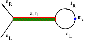
Figure 11: A down quark mass can induce an effective mass for the up quark.

Proceeding further through chiral perturbation theory, one can explore the qualitative phase diagram shown in Fig. 12 for the two flavor theory as a function of the up and down quark masses, including the CP violating Dashen phase Creutz (2011). This figure has some interesting symmetries. First of all, it is symmetric on exchanging the up and down quarks. This is related to isospin and protects the quark mass difference $m_{d}-m_{u}$ from additive renormalization; i.e if the quarks are degenerate, they remain so through the regularization process. It is also symmetric under flipping the sign of both quark masses, $(m_{u},m_{d})\rightarrow(-m_{u},-m_{d})$. This is a consequence of the flavored chiral symmetry $\psi\rightarrow e^{i\pi\tau_{3}\gamma_{5}}\psi$, a good symmetry since $\tau_{3}$ is traceless. This in turn protects the average quark mass from an additive renormalization.

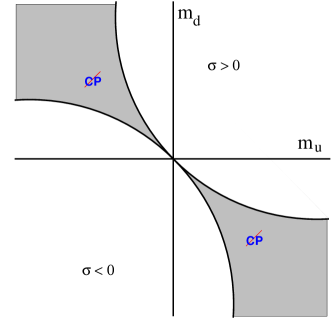
Figure 12: The qualitative phase diagram of two flavor QCD as a function of the quark masses. Here $\sigma$ represents to the quark condensate $\langle\overline{\psi}\psi\rangle$.

It is important, however, to note the absence of any symmetry on flipping the sign of a single quark mass, for example $(m_{u},m_{d})\rightarrow(-m_{u},m_{d})$. Away from $m_{d}=0$ there is no singularity at $m_{u}=0$. This is a strictly non-perturbative effect and shows that a non-degenerate massless quark is not protected from renormalization. Should we care if the concept of a single vanishing quark mass is a bit fuzzy? This quantity is not directly measured in any scattering process. This issue is closely tied to the ambiguities in defining gauge field topology since typical gauge fields are non-differentiable Only real particle masses and their scatterings are physical.

XI Conclusion

Going beyond perturbation theory is crucial for understanding QCD. Lattice gauge theory augmented with ideas from renormalization merge to give a coherent picture accommodating non-perturbative concepts such as confinement and chiral symmetry breaking. Variations of QCD with identical perturbative expansions can display different physics. This includes the situation of a non-vanishing Theta as well as the peculiar possibility of negative quark masses. Finally, the numerical values of the quark masses, as well as their ratios, can depend subtlely on the details of the regularization scheme.

References

- Capitani et al. (2011) Capitani, S., M. Della Morte, G. von Hippel, B. Knippschild, and H. Wittig (2011), PoS LATTICE2011, 145.
- Caswell (1974) Caswell, W. E. (1974), Phys.Rev.Lett. 33, 244.
- Coleman and Weinberg (1973) Coleman, S. R., and E. J. Weinberg (1973), Phys.Rev. D7, 1888.
- Creutz (1980) Creutz, M. (1980), Phys. Rev. D21, 2308.
- Creutz (2011) Creutz, M. (2011), Phys. Rev. D83, 016005.
- Creutz (2018) Creutz, M. (2018), From Quarks to Pions (WSP).
- Dashen (1969) Dashen, R. F. (1969), Phys. Rev. 183, 1245.
- Dashen (1971) Dashen, R. F. (1971), Phys.Rev. D3, 1879.
- Durr et al. (2011) Durr, S., Z. Fodor, C. Hoelbling, S. Katz, S. Krieg, et al. (2011), Phys.Lett. B701, 265.
- Dyson (1952) Dyson, F. (1952), Phys.Rev. 85, 631.
- Feynman (1948) Feynman, R. (1948), Rev.Mod.Phys. 20, 367.
- Fujikawa (1979) Fujikawa, K. (1979), Phys.Rev.Lett. 42, 1195.
- Georgi and Politzer (1976) Georgi, H., and H. Politzer (1976), Phys. Rev. D 14, 1829.
- Gross and Wilczek (1973) Gross, D., and F. Wilczek (1973), Phys.Rev. D8, 3633.
- ’t Hooft (1976) ’t Hooft, G. (1976), Phys.Rev. D14, 3432.
- Jones (1974) Jones, D. (1974), Nucl.Phys. B75, 531.
- Kaplan and Manohar (1986) Kaplan, D. B., and A. V. Manohar (1986), Phys.Rev.Lett. 56, 2004.
- Neuberger (1998) Neuberger, H. (1998), Phys.Lett. B417, 141.
- Politzer (1973) Politzer, H. D. (1973), Phys. Rev. Lett. 30, 1346.
- Wilson (1974) Wilson, K. G. (1974), Phys. Rev. D10, 2445.
- Wilson (1977) Wilson, K. G. (1977), Erice Lectures 1975 New Phenomena In Subnuclear Physics. Part A. Proceedings of the First Half of the 1975 International School of Subnuclear Physics, Erice, Sicily, July 11 - August 1, 1975, ed. A. Zichichi, Plenum Press, New York, 1977, p. 69, CLNS-321.
- Yang and Mills (1954) Yang, C.-N., and R. L. Mills (1954), Phys.Rev. 96, 191.