Online Optimal Control with Affine Constraints

Abstract

This paper considers online optimal control with affine constraints on the states and actions under linear dynamics with bounded random disturbances. The system dynamics and constraints are assumed to be known and time invariant but the convex stage cost functions change adversarially. To solve this problem, we propose Online Gradient Descent with Buffer Zones (OGD-BZ). Theoretically, we show that OGD-BZ with proper parameters can guarantee the system to satisfy all the constraints despite any admissible disturbances. Further, we investigate the policy regret of OGD-BZ, which compares OGD-BZ’s performance with the performance of the optimal linear policy in hindsight. We show that OGD-BZ can achieve a policy regret upper bound that is square root of the horizon length multiplied by some logarithmic terms of the horizon length under proper algorithm parameters.

Introduction

Recently, there is a lot of interest in solving control problems by learning-based techniques, e.g. online learning and reinforcement learning (Agarwal et al. 2019; Li, Chen, and Li 2019; Ibrahimi, Javanmard, and Roy 2012; Dean et al. 2018; Fazel et al. 2018; Yang et al. 2019; Li et al. 2019a). This is motivated by applications such as data centers (Lazic et al. 2018; Li et al. 2019b), robotics (Fisac et al. 2018), autonomous vehicles (Sallab et al. 2017), power systems (Chen et al. 2021), etc. For real-world implementation, it is crucial to design safe algorithms that ensure the system to satisfy certain (physical) constraints despite unknown disturbances. For example, temperatures in data centers should be within certain ranges to reduce task failures despite disturbances from unmodeled heat sources, quadrotors should avoid collisions even when perturbed by wind, etc. In addition to safety, many applications involve time-varying environments, e.g. varying electricity prices, moving targets, etc. Hence, safe algorithms should not be over-conservative and should adapt to varying environments for desirable performance.

In this paper, we design safe algorithms for time-varying environments by considering the following constrained online optimal control problem. Specifically, we consider a linear system with random disturbances,

$$x_{t+1}=Ax_{t}+Bu_{t}+w_{t},\quad t\geq 0,$$ (1)

where disturbance $w_{t}$ is random and satisfies $\|w_{t}\|_{\infty}\leq\bar{w}$. Consider affine constraints on the state $x_{t}$ and the action $u_{t}$:

$$D_{x}x_{t}\leq d_{x},\quad D_{u}u_{t}\leq d_{u},\quad\forall\ t\geq 0.$$ (2)

For simplicity, we assume the system parameters $A,B,\bar{w}$ and the constraints are known. At stage $0\leq t\leq T$, a convex cost function $c_{t}(x_{t},u_{t})$ is adversarially generated and the decision maker selects a feasible action $u_{t}$ before $c_{t}(x_{t},u_{t})$ is revealed. We aim to achieve two goals simultaneously: (i) to minimize the sum of the adversarially varying costs, (ii) to satisfy the constraints (2) for all $t$ despite the disturbances.

There are many studies to address each goal separately but lack results on both goals together as discussed below.

Firstly, there is recent progress on online optimal control to address Goal (i). A commonly adopted performance metric is policy regret, which compares the online cost with the cost of the optimal linear policy in hindsight (Agarwal et al. 2019). Sublinear policy regrets have been achieved for linear systems with either stochastic disturbances (Cohen et al. 2018; Agarwal, Hazan, and Singh 2019) or adversarial disturbances (Agarwal et al. 2019; Foster and Simchowitz 2020; Goel and Hassibi 2020a, b). However, most literature only considers the unconstrained control problem. Recently, Nonhoff and Müller (2020) studies constrained online optimal control but assumes no disturbances.

Secondly, there are many papers from the control community to address Goal (ii): constraints satisfaction. Perhaps the most famous algorithms are Model Predictive Control (MPC) (Rawlings and Mayne 2009) and its variants, such as robust MPC which guarantees (hard) constraint satisfaction in the presence of disturbances (Bemporad and Morari 1999; Kouvaritakis, Rossiter, and Schuurmans 2000; Mayne, Seron, and Raković 2005; Limon et al. 2010; Zafiriou 1990) as well as stochastic MPC which considers soft constraints and allows constraints violation (Oldewurtel, Jones, and Morari 2008; Mesbah 2016). However, there lack algorithms with both regret/optimality guarantees and constraint satisfaction guarantees.

Therefore, an important question remains to be addressed: Q: how to design online algorithms to both satisfy the constraints despite disturbances and yield $o(T)$ policy regrets?

Our Contributions

In this paper, we answer the question above by proposing an online control algorithm: Online Gradient Descent with Buffer Zones (OGD-BZ). To develop OGD-BZ, we first convert the constrained online optimal control problem into an online convex optimization (OCO) problem with temporal-coupled stage costs and temporal-coupled stage constraints, and then convert the temporal-coupled OCO problem into a classical OCO problem. The problem conversion leverages the techniques from recent unconstrained online control literature and robust optimization literature. Since the conversion is not exact/equivalent, we tighten the constraint set by adding buffer zones to account for approximation errors caused by the problem conversion. We then apply classical OCO method OGD to solve the problem and call the resulting algorithm as OGD-BZ.

Theoretically, we show that, with proper parameters, OGD-BZ can ensure all the states and actions to satisfy the constraints (2) for any disturbances bounded by $\bar{w}$. In addition, we show that OGD-BZ’s policy regret can be bounded by $\tilde{O}(\sqrt{T})$ for general convex cost functions $c_{t}(x_{t},u_{t})$ under proper assumptions and parameters. As far as we know, OGD-BZ is the first algorithm with theoretical guarantees on both sublinear policy regret and robust constraint satisfaction. Further, our theoretical results explicitly characterize a trade-off between the constraint satisfaction and the low regret when deciding the size of the buffer zone of OGD-BZ. That is, a larger buffer zone, which indicates a more conservative search space, is preferred for constraints satisfaction; while a smaller buffer zone is preferred for low regret.

Related Work

We provide more literature review below.

Safe reinforcement learning. There is a rich body of literature on safe RL and safe learning-based control that studies how to learn optimal policies without violating constraints and without knowing the system (Fisac et al. 2018; Aswani et al. 2013; Wabersich and Zeilinger 2018; Garcıa and Fernández 2015; Cheng et al. 2019; Zanon and Gros 2019; Fulton and Platzer 2018). Perhaps the most relevant paper is Dean et al. (2019b), which proposes algorithms to learn optimal linear policies for a constrained linear quadratic regulator problem. However, most theoretical guarantees in the safe RL literature require time-invariant environment and there lacks policy regret analysis when facing time-varying objectives. This paper addresses the time-varying objectives but considers known system dynamics. It is our ongoing work to combine both safe RL and our approach to design safe learning algorithms with policy regret guarantees in time-varying problems.

Another important notion of safety is the system stability, which is also studied in the safe RL/learning-based control literature (Dean et al. 2018, 2019a; Chow et al. 2018).

Online convex optimization (OCO). Hazan (2019) provides a review on classical (decoupled) OCO. OCO with memory considers coupled costs and decoupled constraints (Anava, Hazan, and Mannor 2015; Li, Qu, and Li 2020; Li and Li 2020). The papers on OCO with coupled constraints usually allow constraint violation (Yuan and Lamperski 2018; Cao, Zhang, and Poor 2018; Kveton et al. 2008). Besides, OCO does not consider system dynamics or disturbances.

Constrained optimal control. Constrained optimal control enjoys a long history of research. Without disturbances, it is known that the optimal controller for linearly constrained linear quadratic regulator is piecewise linear (Bemporad et al. 2002). With disturbances (as considered in this paper), the problem is much more challenging. Current methods such as robust MPC (Limon et al. 2008, 2010; Rawlings and Mayne 2009) and stochastic MPC (Mesbah 2016; Oldewurtel, Jones, and Morari 2008) usually deploy linear policies for fast computation even though linear policies are suboptimal. Besides, most theoretical analysis of robust/stochastic MPC focus on stability, recursive feasibility, and constraints satisfaction, instead of policy regrets.

Notations and Conventions

We let $\|\cdot\|_{1},\|\cdot\|_{2},\|\cdot\|_{\infty}$ denote the $L_{1},L_{2},L_{\infty}$ norms respectively for vectors and matrices. Let $\mathds{1}_{n}$ denote an all-one vector in $\mathbb{R}^{n}$. For two vectors $a,b\in\mathbb{R}^{n}$, we write $a\leq b$ if $a_{i}\leq b_{i}$ for any entry $i$. Let $\text{vec}(A)$ denote the vectorization of matrix $A$. For better exposition, some bounds use $\Theta(\cdot)$ to omit constants that do not depend on $T$ or the problem dimensions explicitly.

Problem Formulation

In this paper, we consider an online optimal control problem with linear dynamics and affine constraints. Specifically, at each stage $t\in\{0,1,\dots,T\}$, an agent observes the current state $x_{t}$ and implements an action $u_{t}$, which incurs a cost $c_{t}(x_{t},u_{t})$. The stage cost function $c_{t}(\cdot,\cdot)$ is generated adversarially and revealed to the agent after the action $u_{t}$ is taken. The system evolves to the next state according to (1), where $x_{0}$ is fixed, $w_{t}$ is a random disturbance bounded by $w_{t}\in\mathcal{W}=\{w\in\mathbb{R}^{n}:\|w\|_{\infty}\leq\bar{w}\}$, and states and actions should satisfy the affine constraints (2). We denote the corresponding constraint sets as

$$\mathcal{X}\!=\!\{x\in\mathbb{R}^{n}\!\!:\!D_{x}x\leq\!d_{x}\},\quad\mathcal{U}\!=\!\{u\in\mathbb{R}^{m}\!\!:\!D_{u}u\leq\!d_{u}\},$$

where $d_{x}\in\mathbb{R}^{k_{x}}$ and $d_{u}\in\mathbb{R}^{k_{u}}$. Define $k_{c}=k_{x}+k_{u}$ as the total number of the constraints.

For simplicity, we consider that the parameters $A,B,\bar{w},D_{x},d_{x},D_{u},d_{u}$ are known a priori and that the initial value satisfies $x_{0}=0$. We leave the study of unknown parameters and general $x_{0}$ for the future.

Definition 1 (Safe controller).

Consider a controller (or an algorithm) $\mathcal{A}$ that chooses action $u_{t}^{\mathcal{A}}\in\mathcal{U}$ based on history states $\{x_{k}^{\mathcal{A}}\}_{k=0}^{t}$ and cost functions $\{c_{k}(\cdot,\cdot)\}_{k=0}^{t-1}$. The controller $\mathcal{A}$ is called safe if $x_{t}^{\mathcal{A}}\in\mathcal{X}$ and $u_{t}^{\mathcal{A}}\in\mathcal{U}$ for all $0\leq t\leq T$ and all disturbances $\{w_{k}\in\mathcal{W}\}_{k=0}^{T}$.

Define the total cost of a safe algorithm/controller $\mathcal{A}$ as:

$$J_{T}(\mathcal{A})=\operatorname*{\mathbb{E}}_{\{w_{k}\}}\left[\sum_{t=0}^{T}c_{t}(x_{t}^{\mathcal{A}},u_{t}^{\mathcal{A}})\right].$$ (3)

Benchmark Policy and Policy Regret

In this paper, we consider linear policies of the form $u_{t}=-Kx_{t}$ as our benchmark policy for simplicity, though the optimal policy for the constrained control of noisy systems may be nonlinear (Rawlings and Mayne 2009). We leave the discussion on nonlinear policies as future work.

Based on (Cohen et al. 2018), we define strong stability, which is a quantitative version of stability and is commonly introduced to ease non-asymptotic regret analysis in the online control literature (Agarwal, Hazan, and Singh 2019; Agarwal et al. 2019).

Definition 2 (Strong Stability).

A linear controller $u_{t}=-Kx_{t}$ is $(\kappa,\gamma)$-strongly stable for $\kappa\geq 1$ and $\gamma\in(0,1]$ if there exists a matrix $L$ and an invertible matrix $Q$ such that $A-BK=Q^{-1}LQ$, with $\|L\|_{2}\leq 1-\gamma$ and $\max(\|Q\|_{2},\|Q^{-1}\|_{2},\|K\|_{2})\leq\kappa$.

As shown in Cohen et al. (2018), strongly stable controllers can be computed efficiently by SDP formulation.

Our benchmark policy class includes any linear controller $u_{t}=-Kx_{t}$ satisfying the conditions below:

$$\mathcal{K}=\{K:\text{$K$ is safe and $(\kappa,\gamma)$-strongly stable}\},$$

where $K$ is called safe if the controller $u_{t}=-Kx_{t}$ is safe according to Definition 1.

The policy regret of online algorithm $\mathcal{A}$ is defined as:

$$\text{Reg}(\mathcal{A})=J_{T}(\mathcal{A})-\min_{K\in\mathcal{K}}J_{T}(K).$$ (4)

Assumptions and Definitions

For the rest of the paper, we define $\kappa_{B}=\max(\|B\|_{2},1)$. In addition, we introduce the following assumptions on the disturbances and the cost functions, which are standard in literature (Agarwal, Hazan, and Singh 2019).

Assumption 1.

$\{w_{t}\}$ are i.i.d. and bounded by $\|w_{t}\|_{\infty}\leq\bar{w}$, where $\bar{w}>0$.

Assumption 2.

For any $t\geq 0$, cost function $c_{t}(x_{t},u_{t})$ is convex and differentiable with respect to $x_{t}$ and $u_{t}$. Further, there exists $G>0$, such that for any $\|x\|_{2}\leq b$, $\|u\|_{2}\leq b$, we have $\|\nabla_{x}c_{t}(x,u)\|_{2}\leq Gb$ and $\|\nabla_{u}c_{t}(x,u)\|_{2}\leq Gb$.

Next, we define strictly and loosely safe controllers.

Definition 3 (Strict and loose safety).

A safe controller $\mathcal{A}$ is called $\epsilon$-strictly safe for some $\epsilon>0$ if $D_{x}x_{t}^{\mathcal{A}}\leq d_{x}-\epsilon\mathds{1}_{k_{x}}$ and $D_{u}u_{t}^{\mathcal{A}}\leq d_{u}-\epsilon\mathds{1}_{k_{u}}$ for all $0\leq t\leq T$ under any disturbance sequence $\{w_{k}\in\mathcal{W}\}_{k=0}^{T}$.

A controller $\mathcal{A}$ is called $\epsilon$-loosely safe for some $\epsilon>0$ if $D_{x}x_{t}^{\mathcal{A}}\leq d_{x}+\epsilon\mathds{1}_{k_{x}}$ and $D_{u}u_{t}^{\mathcal{A}}\leq d_{u}+\epsilon\mathds{1}_{k_{u}}$ for all $0\leq t\leq T$ under any disturbance sequence $\{w_{k}\in\mathcal{W}\}_{k=0}^{T}$.

In the following, we assume the existence of a strictly safe linear policy. The existence of a safe linear policy is necessary since otherwise our policy regret is not well-defined. The existence of a strictly safe policy provides some flexibility for the approximation steps in our algorithm design and is a common assumption in constrained optimization and control (Boyd and Vandenberghe 2004; Limon et al. 2010).

Assumption 3.

There exists $K_{*}\in\mathcal{K}$ such that the policy $u_{t}=-K_{*}x_{t}$ is $\epsilon_{*}$-strictly safe for some $\epsilon_{*}>0$.

Intuitively, Assumption 3 requires the sets $\mathcal{X}$ and $\mathcal{U}$ to have non-empty interiors and that the disturbance set $\mathcal{W}$ is small enough so that a disturbed linear system $x_{t+1}=(A-BK_{*})x_{t}+w_{t}$ stays in the interiors of $\mathcal{X}$ and $\mathcal{U}$ for any $\{w_{k}\in\mathcal{W}\}_{k=0}^{T}$. In addition, Assumption 3 implicitly assumes that 0 belongs to the interiors of $\mathcal{X}$ and $\mathcal{U}$ since we let $x_{0}=0$. Finally, though it is challenging to verify Assumption 3 directly, there are numerical verification methods, e.g. by solving linear matrix inequalities (LMI) programs (Limon et al. 2010).

Preliminaries

This section briefly reviews the unconstrained online optimal control and robust constrained optimization literature, techniques from which motivate our algorithm design.

Unconstrained Online Optimal Control

In our setting, if one considers $\mathcal{X}=\mathbb{R}^{n}$ and $\mathcal{U}=\mathbb{R}^{m}$, then the problem reduces to an unconstrained online optimal control. For such unconstrained online control problems, Agarwal, Hazan, and Singh (2019); Agarwal et al. (2019) propose a disturbance-action policy class to design an online policy.

Definition 4 (Disturbance-Action Policy (Agarwal, Hazan, and Singh 2019)).

Fix an arbitrary $(\kappa,\gamma)$-strongly stable matrix $\mathbb{K}$ a priori. Given an $H\in\left\{1,2,\ldots,T\right\}$, a disturbance-action policy defines the control policy as:

$$u_{t}=-\mathbb{K}x_{t}+\sum_{i=1}^{H}M^{[i]}w_{t-i},\quad\ \forall\,t\geq 0,$$ (5)

where, $M^{[i]}\in\mathbb{R}^{m\times n}$ and $w_{t}=0$ for $t\leq 0$. Let $\bm{M}=\{M^{[i]}\}_{i=1}^{H}$ denote the list of parameter matrices for the disturbance-action policy.

For the rest of the paper, we will fix $\mathbb{K}$ and discuss how to choose parameter $\bm{M}$. In Agarwal, Hazan, and Singh (2019), a bounded convex constraint set on policy $\bm{M}$ is introduced for technical simplicity and without loss of generality:

$$\mathcal{M}_{2}\!=\!\{\bm{M}\!=\!\{M^{[i]}\}_{i=1}^{H}\!:\!\|M^{[i]}\|_{2}\!\leq\!\kappa^{3}\kappa_{B}(1\!-\!\gamma)^{i},\forall i\}$$ (6)

The next proposition introduces state and action approximations when implementing disturbance-action policies.

Proposition 1 ((Agarwal et al. 2019)).

When implementing a disturbance-action policy (5) with time-varying $\bm{M}_{t}=\{M_{t}^{[i]}\}_{i=1}^{H}$ at each stage $t\geq 0$, the states and actions satisfy:

$$x_{t}=A_{\mathbb{K}}^{H}x_{t-H}+\tilde{x}_{t}\ \ \text{and }\ u_{t}=-\mathbb{K}A_{\mathbb{K}}^{H}x_{t-H}+\tilde{u}_{t},$$ (7)

where $A_{\mathbb{K}}=A-B\mathbb{K}$. The approximate/surrogate state and action, $\tilde{x}_{t}$ and $\tilde{u}_{t}$, are defined as:

$$\tilde{x}_{t}=\sum_{k=1}^{2H}\Phi_{k}^{x}(\bm{M}_{t-H:t-1})w_{t-k},$$

$$\tilde{u}_{t}=-\mathbb{K}\tilde{x}_{t}+\sum_{i=1}^{H}M_{t}^{[i]}w_{t-i}=\sum_{k=1}^{2H}\Phi_{k}^{u}(\bm{M}_{t-H:t})w_{t-k},$$

$$\Phi_{k}^{x}(\bm{M}_{t-H:t-1})\!=\!A_{\mathbb{K}}^{k\!-\!1}\mathds{1}_{(k\!\leq\!H)}\!+\!\sum_{i=1}^{H}\!A_{\mathbb{K}}^{i\!-\!1}BM_{t\!-\!i}^{[k\!-\!i]}\mathds{1}_{(1\!\leq\!k\!-\!i\!\leq\!H)}$$

$$\Phi_{k}^{u}(\bm{M}_{t-H:t})=M_{t}^{[k]}\mathds{1}_{(k\leq H)}-\mathbb{K}\Phi_{k}^{x}(\bm{M}_{t-H:t-1}),$$

where $\bm{M}_{t-H:t}\coloneqq\{\bm{M}_{t-H},\dots,\bm{M}_{t}\}$, the superscript $k$ in $A_{\mathbb{K}}^{k}$ denotes the $k$th power of $A_{\mathbb{K}}$, and $M_{t}^{[k]}$ with superscript $[k]$ denotes the $k$th matrix in list $\bm{M}_{t}$. Further, define $\mathring{\Phi}_{k}^{x}(\bm{M})=\Phi_{k}^{x}(\bm{M},\dots,\bm{M}),\,\mathring{\Phi}_{k}^{u}(\bm{M})=\Phi_{k}^{u}(\bm{M},\dots,\bm{M})$.

Notice that $\tilde{x}_{t}$ and $\tilde{u}_{t}$ are affine functions of $\bm{M}_{t-H:t}$. Based on $\tilde{x}_{t}$ and $\tilde{u}_{t}$, Agarwal, Hazan, and Singh (2019) introduces an approximate cost function:

$$f_{t}(\bm{M}_{t-H:t})=\operatorname*{\mathbb{E}}[c_{t}(\tilde{x}_{t},\tilde{u}_{t})],$$

which is convex with respect to $\bm{M}_{t-H:t}$ since $\tilde{x}_{t}$ and $\tilde{u}_{t}$ are affine functions of $\bm{M}_{t-H:t}$ and $c_{t}(\cdot,\cdot)$ is convex.

Remark 1.

The disturbance-action policy is related to affine disturbance feedback in stochastic MPC (Oldewurtel, Jones, and Morari 2008; Mesbah 2016), which also considers policies that are linear with disturbances to convexify the control problem in MPC’s lookahead horizon.

OCO with memory. In Agarwal, Hazan, and Singh (2019), the unconstrained online optimal control problem is converted into OCO with memory, i.e. at each stage $t$, the agent selects a policy $\bm{M}_{t}\in\mathcal{M}_{2}$ and then incurs a cost $f_{t}(\bm{M}_{t-H:t})$. Notice that the cost function at stage $t$ couples the current policy $\bm{M}_{t}$ with the $H$-stage historical policies $\bm{M}_{t-H:t-1}$, but the constraint set $\mathcal{M}_{2}$ is decoupled and only depends on the current $\bm{M}_{t}$.

To solve this “OCO with memory” problem, Agarwal, Hazan, and Singh (2019) defines decoupled cost functions

$$\mathring{f}_{t}(\bm{M}_{t})\coloneqq f_{t}(\bm{M}_{t},\dots,\bm{M}_{t}),$$ (8)

by letting the $H$-stage historical policies be identical to the current policy. Notice that $\mathring{f}_{t}(\bm{M}_{t})$ is still convex. Accordingly, the OCO with memory is reformulated as a classical OCO problem with stage cost $\mathring{f}_{t}(\bm{M}_{t})$, which is solved by classical OCO algorithms such as online gradient descent (OGD) in Agarwal, Hazan, and Singh (2019). The stepsizes of OGD are chosen to be sufficiently small so that the variation between the current policy $\bm{M}_{t}$ and the $H$-stage historical policies $\bm{M}_{t-H},\dots,\bm{M}_{t-1}$ is sufficiently small, which guarantees a small approximation error between $\mathring{f}_{t}(\bm{M}_{t})$ and $f_{t}(\bm{M}_{t-H:t})$, and thus low regrets. For more details, we refer the reader to Agarwal, Hazan, and Singh (2019).

Robust Optimization with Constraints

Consider a robust optimization problem with linear constraints (Ben-Tal, El Ghaoui, and Nemirovski 2009):

$$\min_{x} \ f(x)\quad\text{s.t. }\ a_{i}^{\top}x\leq b_{i},\ \forall\,a_{i}\in\mathcal{C}_{i},\ \forall\,1\leq i\leq k,$$ (9)

where the (box) uncertainty sets are defined as $\mathcal{C}_{i}=\{a_{i}\!=\!\tilde{a}_{i}\!+\!P_{i}z\!:\!\|z\|_{\infty}\!\leq\!\bar{z}\}$ for any $i$. Notice that the robust constraint $\{a_{i}^{\top}x\leq b_{i},\ \forall\,a_{i}\in\mathcal{C}_{i}\}$ is equivalent to the standard constraint $\{\sup_{a_{i}\in\mathcal{C}_{i}}[a_{i}^{\top}x]\leq b_{i}\}$. Further, one can derive

$$\sup_{a_{i}\in\mathcal{C}_{i}}a_{i}^{\top}x=\sup_{\|z\|_{\infty}\leq\bar{z}}(\tilde{a}_{i}+P_{i}z)^{\top}x$$

$$=\ \tilde{a}_{i}^{\top}x+\sup_{\|z\|_{\infty}\leq\bar{z}}z^{\top}(P_{i}^{\top}x)=\tilde{a}_{i}^{\top}x+\|P_{i}^{\top}x\|_{1}\bar{z}$$ (10)

Therefore, the robust optimization (9) can be equivalently reformulated as the linearly constrained optimization below:

$$\min_{x} \ f(x)\quad\text{s.t. }\ \tilde{a}_{i}^{\top}x+\|P_{i}^{\top}x\|_{1}\bar{z}\leq b_{i},\ \forall\,1\leq i\leq k.$$

Online Algorithm Design

This section introduces our online algorithm design for online disturbance-action policies (Definition 4).

Roughly speaking, to develop our online algorithm, we first convert the constrained online optimal control into OCO with memory and coupled constraints, which is later converted into classical OCO and solved by OCO algorithms. The conversions leverage the approximation and the reformulation techniques in the Preliminaries. During the conversions, we ensure that the outputs of the OCO algorithms are safe for the original control problem. This is achieved by tightening the original constraints (adding buffer zones) to allow for approximation errors. Besides, our method ensures small approximation errors and thus small buffer zones so that the optimality/regret is not sacrificed significantly for safety. The details of algorithm design are discussed below.

Step 1: Constraints on Approximate States and Actions

When applying the disturbance-action policies (5), we can use (7) to rewrite the state constraint $x_{t+1}\in\mathcal{X}$ as

$$D_{x}A_{\mathbb{K}}^{H}x_{t-H+1}+D_{x}\tilde{x}_{t+1}\leq d_{x},\ \ \forall\,\{w_{k}\in\mathcal{W}\}_{k=0}^{T},$$ (11)

where $\tilde{x}_{t+1}$ is the approximate state. Note that the term $D_{x}A_{\mathbb{K}}^{H}x_{t-H+1}$ decays exponentially with $H$. If there exists $H$ such that $D_{x}A_{\mathbb{K}}^{H}x_{t-H+1}\leq\epsilon_{1}\mathds{1}_{k_{x}}$, $\forall\,\{w_{k}\in\mathcal{W}\}_{k=0}^{T}$, then a tightened constraint on the approximate state, i.e.

$$D_{x}\tilde{x}_{t+1}\leq d_{x}-\epsilon_{1}\mathds{1}_{k_{x}},\quad\forall\,\{w_{k}\in\mathcal{W}\}_{k=0}^{T},$$ (12)

can guarantee the original constraint on the true state (11).

The action constraint $u_{t}\in\mathcal{U}$ can similarly be converted into a tightened constraint on the approximate action $\tilde{u}_{t}$, i.e.

$$D_{u}\tilde{u}_{t}\leq d_{u}-\epsilon_{1}\mathds{1}_{k_{u}},\quad\forall\,\{w_{k}\in\mathcal{W}\}_{k=0}^{T},$$ (13)

if $D_{u}(-\mathbb{K}A_{\mathbb{K}}^{H}x_{t-H})\leq\epsilon_{1}\mathds{1}_{k_{u}}$ for any $\{w_{k}\in\mathcal{W}\}_{k=0}^{T}$.

Step 2: Constraints on the Policy Parameters

Next, we reformulate the robust constraints (12) and (13) on $\tilde{x}_{t+1}$ and $\tilde{u}_{t}$ as polytopic constraints on policy parameters $\bm{M}_{t-H:t}$ based on the robust optimization techniques reviewed in Robust Optimization with Constraints.

Firstly, we consider the $i$th row of the constraint (12), i.e. $D_{x,i}^{\top}\tilde{x}_{t+1}\leq d_{x,i}-\epsilon_{1}$ $\forall\,\{w_{k}\in\mathcal{W}\}_{k=0}^{T},$ where $D_{x,i}^{\top}$ denotes the $i$th row of the matrix $D_{x}$. This constraint is equivalent to $\sup_{\{w_{k}\in\mathcal{W}\}_{k=0}^{T}}(D_{x,i}^{\top}\tilde{x}_{t+1})\leq d_{x,i}-\epsilon_{1}$. Further, by (10) and the definitions of $\tilde{x}_{t+1}$ and $\mathcal{W}$, we obtain

$$\sup_{\{w_{k}\!\in\!\mathcal{W}\}}\!D_{x,i}^{\top}\tilde{x}_{t+1}\! =\!\sup_{\{w_{k}\in\mathcal{W}\}}D_{x,i}^{\top}\sum_{s=1}^{2H}\Phi^{x}_{s}(\bm{M}_{t-H+1:t})w_{t\!+\!1\!-\!s}$$

$$=\!\sum_{s=1}^{2H}\!\sup_{w_{t\!+\!1\!-\!s}\in\mathcal{W}}\!D_{x,i}^{\top}\Phi^{x}_{s}(\bm{M}_{t-H+1:t})w_{t\!+\!1\!-\!s}$$

$$=\sum_{s=1}^{2H}\|D_{x,i}^{\top}\Phi^{x}_{s}(\bm{M}_{t-H+1:t})\|_{1}\bar{w}$$

Define $g_{i}^{x}(\bm{M}_{t-H+1:t})=\sum_{s=1}^{2H}\|D_{x,i}^{\top}\Phi^{x}_{s}(\bm{M}_{t-H+1:t})\|_{1}\bar{w}.$ Hence, the robust constraint (12) on $\tilde{x}_{t+1}$ is equivalent to the following polytopic constraints on $\bm{M}_{t-H+1:t}$:

$$g_{i}^{x}(\bm{M}_{t-H+1:t})\leq d_{x,i}-\epsilon_{1},\quad\forall\,1\leq i\leq k_{x}.$$ (14)

Similarly, the constraint (13) on $\tilde{u}_{t}$ is equivalent to:

$$g_{j}^{u}(\bm{M}_{t-H:t})\leq d_{u,j}-\epsilon_{1},\quad\forall\,1\leq j\leq k_{u},$$ (15)

where $g_{j}^{u}(\bm{M}_{t-H:t})=\sum_{s=1}^{2H}\|D_{u,j}^{\top}\Phi^{u}_{s}(\bm{M}_{t-H:t})\|_{1}\bar{w}.$

Step 3: OCO with Memory and Temporal-coupled Constraints

By Step 2 and our review of robust optimization, we can convert the constrained online optimal control problem into OCO with memory and coupled constraints. That is, at each $t$, the decision maker selects a policy $\bm{M}_{t}$ satisfying constraints (14) and (15), and then incurs a cost $f_{t}(\bm{M}_{t-H:t})$. In our framework, both the constraints (14), (15) and the cost function $f_{t}(\bm{M}_{t-H:t})$ couple the current policy with the historical policies. This makes the problem far more challenging than OCO with memory which only considers coupled costs (Anava, Hazan, and Mannor 2015).

Step 4: Benefits of the Slow Variation of Online Policies

We approximate the coupled constraint functions $g^{x}_{i}(\bm{M}_{t-H+1:t})$ and $g^{u}_{j}(\bm{M}_{t-H:t})$ as decoupled ones below,

$$\mathring{g}^{x}_{i}(\bm{M}_{t})\!=\!g^{x}_{i}(\bm{M}_{t},\dots,\bm{M}_{t}),\mathring{g}^{u}_{i}(\bm{M}_{t})\!=\!g^{u}_{i}(\bm{M}_{t},\dots,\bm{M}_{t}),$$

by letting the historical policies $\bm{M}_{t-H:t-1}$ be identical to the current $\bm{M}_{t}$. If the online policy $\bm{M}_{t}$ varies slowly with $t$, which is satisfied by most OCO algorithms (e.g. OGD with a diminishing stepsize (Hazan 2019)), one may be able to bound the approximation errors by $g^{x}_{i}(\bm{M}_{t-H+1:t})-\mathring{g}^{x}_{i}(\bm{M}_{t})\leq\epsilon_{2}$ and $g^{u}_{j}(\bm{M}_{t-H:t})-\mathring{g}^{u}_{j}(\bm{M}_{t})\leq\epsilon_{2}$ for a small $\epsilon_{2}>0$. Consequently, the constraints (14) and (15) are ensured by the polytopic constraints that only depend on $\bm{M}_{t}$:

$$\mathring{g}^{x}_{i}(\bm{M}_{t})\leq\!d_{x,i}\!-\epsilon_{1}-\epsilon_{2},\ \mathring{g}^{u}_{j}(\bm{M}_{t})\leq\!d_{u,j}\!-\epsilon_{1}-\epsilon_{2},$$ (16)

where the buffer zone $\epsilon_{2}$ allows for the approximation error caused by neglecting the variation of the online policies.

Step 5: Conversion to OCO

By Step 4, we define a decoupled search space/constraint set on each policy below,

$$\Omega_{\epsilon}\!=\!\{\bm{M}\in\mathcal{M}: \ \mathring{g}^{x}_{i}(\bm{M})\leq d_{x,i}-\epsilon,\forall 1\leq i\leq k_{x},$$ (17)

$$\mathring{g}^{u}_{j}(\bm{M})\leq d_{u,j}-\epsilon,\forall\,1\leq j\leq k_{u}\},$$

where $\mathcal{M}$ is a bounded convex constraint set defined as

$$\mathcal{M}=\{\bm{M}:\ \|M^{[i]}\|_{\infty}\leq 2\sqrt{n}\kappa^{3}(1-\gamma)^{i-1},\ \forall\,1\leq i\leq H\}.$$

Our set $\mathcal{M}$ is slightly different from $\mathcal{M}_{2}$ in (6) to ensure that $\Omega_{\epsilon}$ is a polytope. Notice that $\Omega_{\epsilon}$ provides buffer zones with size $\epsilon$ to account for the approximation errors $\epsilon_{1}$ and $\epsilon_{2}$. Based on $\Omega_{\epsilon}$ and technique (8), we can further convert the “OCO with memory and coupled constraints” in Step 3 into a classical OCO problem below. That is, at each $t$, the agent selects a policy $\bm{M}_{t}\in\Omega_{\epsilon}$, and then suffers a convex stage cost $\mathring{f}_{t}(\bm{M}_{t})$ defined in (8). We apply online gradient descent to solve this OCO problem, as described in Algorithm 1. We select the stepsizes of OGD to be small enough to ensure small approximation errors from Step 4 and thus small buffer zones, but also to be large enough to allow online policies to adapt to time-varying environments. Conditions for suitable stepsizes are discussed in Theoretical Results.

Input: A $(\kappa,\gamma)$-strongly stable matrix $\mathbb{K}$, parameter $H>0$, buffer size $\epsilon$, stepsize $\eta_{t}$.

1

2Determine the polytopic constraint set $\Omega_{\epsilon}$ by (17) with buffer size $\epsilon$ and initialize $\bm{M}_{0}\in\Omega_{\epsilon}$.

3

4for $t=0,1,2,\ldots,T$ do

5      Implement action $u_{t}=-\mathbb{K}x_{t}\!+\!\sum_{i=1}^{H}M_{t}^{[i]}w_{t-i}.$

6     

7     Observe the next state $x_{t+1}$ and record $w_{t}=x_{t+1}-Ax_{t}-Bu_{t}$.

8     

9     Run projected OGD

$$\bm{M}_{t+1}=\Pi_{\Omega_{\epsilon}}\left[\bm{M}_{t}-\eta_{t}\nabla\mathring{f}_{t}(\bm{M}_{t})\right]$$

where $\mathring{f}_{t}(\bm{M})$ is defined in (8).

10     

Algorithm 1 OGD-BZ

In Algorithm 1, the most computationally demanding step at each stage is the projection onto the polytope $\Omega_{\epsilon}$, which requires solving a quadratic program. Nevertheless, one can reduce the online computational burden via offline computation by leveraging the solution structure of quadratic programs (see (Alessio and Bemporad 2009) for more details).

Lastly, we note that other OCO algorithms can be applied to solve this problem too, e.g. online natural gradient, online mirror descent, etc. One can also apply projection-free methods, e.g. (Yuan and Lamperski 2018), to reduce the computational burden at the expense of $o(T)$ constraint violation.

Remark 2.

To ensure safety, safe RL literature usually constructs a safe set for the state (Fisac et al. 2018), while this paper constructs a safe search space $\Omega_{\epsilon}$ for the policies directly. Besides, safe RL literature may employ unsafe policies occasionally, for example, Fisac et al. (2018) allows unsafe exploration policies within the safe set and changes to a safe policy on the boundary of the safe set. However, our search space $\Omega_{\epsilon}$ only contains safe policies. Despite a smaller policy search space, our OGD-BZ still achieves desirable (theoretical) performance. Nevertheless, when the system is unknown, larger sets of exploration policies may benefit the performance, which is left as future work.

Remark 3.

It is worth comparing our method with a well-known robust MPC method: tube-based robust MPC (see e.g. Rawlings and Mayne (2009)). Tube-based robust MPC also tightens the constraints to allow for model inaccuracy and/or disturbances. However, tube-based robust MPC considers constraints on the states, while our method converts the state (and action) constraints into the constraints on the policy parameters by leveraging the properties of disturbance-action policies.

Theoretical Results

In this section, we show that OGD-BZ guarantees both safety and $\tilde{O}(\sqrt{T})$ policy regret under proper parameters.

Preparation

To establish the conditions on the parameters for our theoretical results, we introduce three quantities $\epsilon_{1}(H),\epsilon_{2}(\eta,H),\epsilon_{3}(H)$ below. We note that $\epsilon_{1}(H)$ and $\epsilon_{2}(\eta,H)$ bound the approximation errors in Step 1 and Step 4 of the previous section respectively (see Lemma 1 and Lemma 3 in the proof of Theorem 1 for more details). $\epsilon_{3}(H)$ bounds the constraint violation of the disturbance-action policy $\bm{M}(K)$, where $\bm{M}(K)$ approximates the linear controller $u_{t}=-Kx_{t}$ for any $K\in\mathcal{K}$ (see Lemma 4 in the proof of Theorem 1 for more details).

Definition 5.

We define

$$\epsilon_{1}(H) =c_{1}n\sqrt{m}H(1-\gamma)^{H},\epsilon_{2}(\eta,H)=c_{2}\eta\cdot n^{2}\sqrt{m}H^{2}$$

$$\epsilon_{3}(H) =c_{3}\sqrt{n}(1-\gamma)^{H}$$

where $c_{1}$, $c_{2}$, and $c_{3}$ are polynomials of $\|D_{x}\|_{\infty},\|D_{u}\|_{\infty}$, $\kappa,\kappa_{B},\gamma^{-1},\bar{w},G$.

Safety of OGD-BZ

Theorem 1 (Feasibility & Safety).

Consider constant stepsize $\eta_{t}=\eta$, $\epsilon\geq 0,H\geq\frac{\log(2\kappa^{2})}{\log((1-\gamma)^{-1})}$. If the buffer size $\epsilon$ and $H$ satisfy

$$\epsilon\leq\epsilon_{*}-\epsilon_{1}(H)-\epsilon_{3}(H),$$

the set $\Omega_{\epsilon}$ is non-empty. Further, if $\eta$, $\epsilon$ and $H$ also satisfy

$$\epsilon\geq\epsilon_{1}(H)+\epsilon_{2}(\eta,H),$$

our OGD-BZ is safe, i.e. $x^{\textup{OGD-BZ}}_{t}\in\mathcal{X}$ and $u_{t}^{\textup{OGD-BZ}}\in\mathcal{U}$ for all $t$ and for any disturbances $\{w_{k}\in\mathcal{W}\}_{k=0}^{T}$.

Discussions: Firstly, Theorem 1 shows that $\epsilon$ should be small enough to ensure a nonempty $\Omega_{\epsilon}$ and thus valid/feasible outputs of OGD-BZ. This is intuitive since the constraints are more conservative as $\epsilon$ increases. Since $\epsilon_{1}(H)+\epsilon_{3}(H)=\Theta(H(1-\gamma)^{H})$ decays with $H$ by Definition 5, the first condition also implies a large enough $H$.

Secondly, Theorem 1 shows that, to ensure safety, the buffer size $\epsilon$ should also be large enough to allow for the total approximation errors $\epsilon_{1}(H)+\epsilon_{2}(\eta,H)$, which is consistent with our discussion in the previous section. To ensure the compatibility of the two conditions on $\epsilon$, the approximation errors $\epsilon_{1}(H)+\epsilon_{2}(\eta,H)$ should be small enough, which requires a large enough $H$ and a small enough $\eta$ by Definition 5.

In conclusion, the safety requires a large enough $H$, a small enough $\eta$, and an $\epsilon$ which is neither too large nor too small. For example, we can select $\eta\leq\frac{\epsilon_{*}}{8c_{2}n^{2}\sqrt{m}H^{2}}$, $\epsilon_{*}/4\leq\epsilon\leq 3\epsilon_{*}/4$, and $H\geq\max(\frac{\log(\frac{8(c_{1}+c_{3})n\sqrt{m}}{\epsilon_{*}}T)}{\log((1-\gamma)^{-1}},\frac{\log(2\kappa^{2})}{\log((1-\gamma)^{-1})})$.

Remark 4.

It can be shown that it is safe to implement any $\bm{M}\in\Omega_{\epsilon}$ for an infinite horizon ($0\leq t\leq+\infty$) under the conditions of Theorem 1 based on the proof of Theorem 1. For more details, please refer to the end of the proof of Theorem 1.

Policy Regret Bound for OGD-BZ

Theorem 2 (Regret Bound).

Under the conditions in Theorem 1, OGD-BZ enjoys the regret bound below:

$$\textup{Reg}(\textup{OGD-BZ})\leq\, O\!\left(n^{3}mH^{3}\eta T+\frac{mn}{\eta}\right.$$

$$+\!(1\!-\!\gamma)^{H}\!H^{2.5}T({n^{{3}}m^{{1.5}}}\!+\!\sqrt{k_{c}}mn^{2.5})/\epsilon_{*}$$

$$+\left.\epsilon TH^{1.5}({n^{{2}}m}+\sqrt{k_{c}mn^{3}})/\epsilon_{*}\right),$$

where the hidden constant depends polynomially on $\kappa,\kappa_{B},$ $\gamma^{-1},{\|D_{x}\|_{\infty},\|D_{u}\|_{\infty},}\|d_{x}\|_{2},\|d_{u}\|_{2},\bar{w},G$.

Theorem 2 provides a regret bound for OGD-BZ as long as OGD-BZ is safe. Notice that as the buffer size $\epsilon$ increases, the regret bound becomes worse. This is intuitive since our OGD-BZ will have to search for policies in a smaller set $\Omega_{\epsilon}$ if $\epsilon$ increases. Consequently, the buffer size $\epsilon$ can serve as a tuning parameter for the trade-off between safety and regrets, i.e. a small $\epsilon$ is preferred for low regrets while a large $\epsilon$ is preferred for safety (as long as $\Omega_{\epsilon}\not=\emptyset$). In addition, although a small stepsize $\eta$ is preferred for safety in Theorem 1, Theorem 2 suggests that the stepsize should not be too small for low regrets since the regret bound contains a $\Theta(\eta^{-1})$ term. This is intuitive since the stepsize $\eta$ should be large enough to allow OGD-BZ to adapt to the varying objectives for better online performance.

Next, we provide a regret bound with specific parameters.

Corollary 1.

For sufficiently large $T$, when $H\geq\frac{\log(8(c_{1}+c_{2})n\sqrt{m}T/\epsilon_{*})}{\log((1-\gamma)^{-1})}$, $\eta=\Theta(\frac{1}{n^{2}\sqrt{m}H\sqrt{T}})$, $\epsilon=\epsilon_{1}(H)+\epsilon_{2}(\eta,H)=\Theta(\frac{\log(n\sqrt{m}T)}{\sqrt{T}})$, OGD-BZ is safe and $\textup{Reg}(\textup{OGD-BZ})\leq\tilde{O}\left((n^{{3}}m^{1.5}{k_{c}}^{0.5})\sqrt{T}\right).$

Corollary 1 shows that OGD-BZ achieves $\tilde{O}(\sqrt{T})$ regrets when $H\geq\Theta(\log T)$, $\eta^{-1}=\tilde{\Theta}(\sqrt{T})$, and $\epsilon=\tilde{\Theta}(1/\sqrt{T})$. This demonstrates that OGD-BZ can ensure both constraint satisfaction and sublinear regrets under the proper parameters of the algorithm. We remark that a larger $H$ is preferred for better performance due to smaller approximation errors and a potentially larger policy search space $\Omega_{\epsilon}$, but the computational complexity of OGD-BZ increases with $H$. Besides, though the choices of $H$, $\eta$, and $\epsilon$ above require the prior knowledge of $T$, one can apply doubling tricks (Hazan 2019) to avoid this requirement. Lastly, we note that our $\tilde{O}(\sqrt{T})$ regret bound is consistent with the unconstrained online optimal control literature for convex cost functions (Agarwal et al. 2019). For strongly convex costs, the regret for the unconstrained case is logarithmic in $T$ (Agarwal, Hazan, and Singh 2019). We leave the study on the constrained control with strongly convex costs for the future.

Proof of Theorem 1

To prove Theorem 1, we first provide lemmas to bound errors by $\epsilon_{1}(H),\epsilon_{2}(\eta,H)$, and $\epsilon_{3}(H)$, respectively. The proofs of Lemmas 1-4 and Corollary 2 in this subsection are provided in the arXiv version (Li, Das, and Li 2020).

Firstly, we show that the approximation error in Step 1 of the previous section can be bounded by $\epsilon_{1}(H)$.

Lemma 1 (Error bound $\epsilon_{1}(H)$).

When $\bm{M}_{k}\in\mathcal{M}$ for all $k$ and $H\geq\frac{\log(2\kappa^{2})}{\log((1-\gamma)^{-1})}$, we have

$$\max_{\|w_{k}\|_{\infty}\leq\bar{w}}\|D_{x}A_{\mathbb{K}}^{H}x_{t-H}\|_{\infty}\leq\epsilon_{1}(H),$$

$$\max_{\|w_{k}\|_{\infty}\leq\bar{w}}\|D_{u}\mathbb{K}A_{\mathbb{K}}^{H}x_{t-H}\|_{\infty}\leq\epsilon_{1}(H).$$

The proof of Lemma 1 relies on the boundedness of $x_{t}$ when implementing $\bm{M}_{t}\in\mathcal{M}$ as stated below.

Lemma 2 (Bound on $x_{t}$).

With $\bm{M}_{k}\in\mathcal{M}$ for all $k$ and $\kappa^{2}(1-\gamma)^{H}<1$, we have

$$\|x_{t}\|_{2}\leq b,$$

where $b=\frac{\kappa\sqrt{n}\bar{w}(\kappa^{2}+2\kappa^{5}\kappa_{B}\sqrt{mn}H)}{(1-\kappa^{2}(1-\gamma)^{H})\gamma}+2\sqrt{mn}\kappa^{3}\bar{w}/\gamma$. Hence, when $H\geq\frac{\log(2\kappa^{2})}{\log((1-\gamma)^{-1})}$, we have $b\leq 8\sqrt{mn^{2}}H\bar{w}\kappa^{6}\kappa_{B}/\gamma$.

Secondly, we show that the error incurred by the Step 3 of the previous section can be bounded by $\epsilon_{2}(\eta,H)$.

Lemma 3 (Error bound $\epsilon_{2}(\eta,H)$).

When $H\geq\frac{\log(2\kappa^{2})}{\log((1-\gamma)^{-1})}$, the policies $\{\bm{M}_{t}\}_{t=0}^{T}$ generated by OGD-BZ with a constant stepsize $\eta$ satisfy

$$\max_{1\leq i\leq k_{x}}|\mathring{g}^{x}_{i}(\bm{M}_{t})-g^{x}_{i}(\bm{M}_{t-H+1:t})|\leq\epsilon_{2}(\eta,H),$$

$$\max_{1\leq j\leq k_{u}}|\mathring{g}^{u}_{j}(\bm{M}_{t})-g^{u}_{j}(\bm{M}_{t-H:t})|\leq\epsilon_{2}(\eta,H).$$

Thirdly, we show that for any $K\in\mathcal{K}$, there exists a disturbance-action policy $\bm{M}(K)\in\mathcal{M}$ to approximate the policy $u_{t}=-Kx_{t}$. However, $\bm{M}(K)$ may not be safe and is only $\epsilon_{3}(H)$-loosely safe.

Lemma 4 (Error bound $\epsilon_{3}(H)$).

For any $K\in\mathcal{K}$, there exists a disturbance-action policy $\bm{M}(K)=\{M^{[i]}(K)\}_{i=1}^{H}\in\mathcal{M}$ defined as $M^{[i]}(K)=(\mathbb{K}-K)(A-BK)^{i-1}$ such that

$$\max(\|{D_{x}}[x_{t}^{K}\!-\!x_{t}^{\bm{M}(K)}\!]\|_{{\infty}},\|{D_{u}}[u_{t}^{K}\!-\!u_{t}^{\bm{M}(K)}\!]\|_{{\infty}})\!\leq\!\epsilon_{3}(H)$$

where $(x_{t}^{K},u_{t}^{K})$ and $(x_{t}^{\bm{M}(K)},u_{t}^{\bm{M}(K)})$ are produced by controller $u_{t}\!=\!-Kx_{t}$ and disturbance-action policy $\bm{M}(K)$ respectively. Hence, $\bm{M}(K)$ is $\epsilon_{3}(H)$-loosely safe.

Based on Lemma 4, we can further show that $\bm{M}(K)$ belongs to a polytopic constraint set in the following corollary. For the rest of the paper, we will omit the arguments in $\epsilon_{1}(H),\epsilon_{2}(\eta,H),\epsilon_{3}(H)$ for notational simplicity.

Corollary 2.

Consider $K\in\mathcal{K}$, if $K$ is $\epsilon_{0}$-strictly safe for $\epsilon_{0}\geq 0$, then $\bm{M}(K)\in\Omega_{\epsilon_{0}-\epsilon_{1}-\epsilon_{3}}.$

Proof of Theorem 1.

For notational simplicity, we denote the states and actions generated by OGD-BZ as $x_{t}$ and $u_{t}$ in this proof. First, we show $\bm{M}(K_{*})\in\Omega_{\epsilon}$ below. Since $K_{*}$ defined in Assumption 3 is $\epsilon_{*}$-strictly safe, by Corollary 2, there exists $\bm{M}(K_{*})\in\Omega_{\epsilon_{*}-\epsilon_{1}-\epsilon_{3}}$. Since the set $\Omega_{\epsilon}$ is smaller as $\epsilon$ increases, when $\epsilon_{*}-\epsilon_{1}-\epsilon_{3}\geq\epsilon$, we have $\bm{M}(K_{*})\in\Omega_{\epsilon_{*}-\epsilon_{1}-\epsilon_{3}}\subseteq\Omega_{\epsilon}$, so $\Omega_{\epsilon}$ is non-empty.

Next, we prove the safety by Lemma 1 and Lemma 3 based on the discussions in the previous section. Specifically, OGD-BZ guarantees that $\bm{M}_{t}\in\Omega_{\epsilon}$ for all $t$. Thus, by Lemma 3, we have $g_{i}^{x}(\bm{M}_{t-H:t-1})=g_{i}^{x}(\bm{M}_{t-H:t-1})-\mathring{g}_{i}^{x}(\bm{M}_{t-1})+\mathring{g}_{i}^{x}(\bm{M}_{t-1})\leq\epsilon_{2}+d_{x,i}-\epsilon$ for any $i$. Further, by Step 2 of the previous section and Lemma 1, we have $D_{x,i}^{\top}x_{t}=D_{x,i}^{\top}A_{\mathbb{K}}^{H}x_{t-H}\!+\!D_{x,i}^{\top}\tilde{x}_{t}\leq\|D_{x}A_{\mathbb{K}}^{H}x_{t-H}\|_{\infty}+g_{i}^{x}(\bm{M}_{t-H:t-1})\leq\epsilon_{1}+\epsilon_{2}+d_{x,i}-\epsilon\leq d_{x,i}$ for any $\{w_{k}\in\mathcal{W}\}_{k=0}^{T}$ if $\epsilon\geq\epsilon_{1}+\epsilon_{2}$. Therefore, $x_{t}\in\mathcal{X}$ for all $w_{k}\in\mathcal{W}$. Similarly, we can show $u_{t}\in\mathcal{U}$ for any $w_{k}\in\mathcal{W}$. Thus, OGD-BZ is safe. ∎

Proof of Remark 4. When implementing $\bm{M}\in\Omega_{\epsilon}$ for an infinite horizon, we have $\mathring{g}_{i}^{x}(\bm{M})=g_{i}^{x}(\bm{M},\dots,\bm{M})\leq d_{x,i}-\epsilon$. Since Proposition 1 holds for any $t\geq 0$, we still have $D_{x,i}^{\top}x_{t}=D_{x,i}^{\top}A_{\mathbb{K}}^{H}x_{t-H}\!+\!D_{x,i}^{\top}\tilde{x}_{t}\leq\|D_{x}A_{\mathbb{K}}^{H}x_{t-H}\|_{\infty}+g_{i}^{x}(\bm{M},\dots,\bm{M})\leq\epsilon_{1}+d_{x,i}-\epsilon\leq d_{x,i}$ for any $\{w_{k}\in\mathcal{W}\}_{k=0}^{T}$ if $\epsilon\geq\epsilon_{1}+\epsilon_{2}$. Thus, $x_{t}\in\mathcal{X}$ for all $w_{k}\in\mathcal{W}$ for $t\geq 0$. Constraint satisfaction of $u_{t}$ can be proved similarly.

Proof of Theorem 2

We divide the regret into three parts and bound each part.

$$\ \text{Reg}(\text{OGD-BZ})=\ J_{T}(\mathcal{A})-\min_{K\in\mathcal{K}}J_{T}(K)$$

$$= \ \underbrace{J_{T}(\mathcal{A})-\sum_{t=0}^{T}\mathring{f}_{t}(\bm{M}_{t})}_{\text{Part i}}+\underbrace{\sum_{t=0}^{T}\mathring{f}_{t}(\bm{M}_{t})-\min_{\bm{M}\in\Omega_{\epsilon}}\sum_{t=0}^{T}\mathring{f}_{t}(\bm{M})}_{\text{Part ii}}$$

$$\ +\underbrace{\min_{\bm{M}\in\Omega_{\epsilon}}\sum_{t=0}^{T}\mathring{f}_{t}(\bm{M})-\min_{K\in\mathcal{K}}J_{T}(K)}_{\text{Part iii}}$$

Bound on Part ii. Firstly, we bound Part ii based on the regret bound of OGD in the literature (Hazan 2019).

Lemma 5.

With a constant stepsize $\eta$, we have $\textup{Part ii}\leq\delta^{2}/{2\eta}+{\eta}G_{f}^{2}T/2$, where $\delta=\sup_{\bm{M},\tilde{\bm{M}}\in\Omega_{\epsilon}}\|\bm{M}-\tilde{\bm{M}}\|_{F}\leq 4\sqrt{mn}\kappa^{3}/\gamma$ and $G_{f}=\max_{t}\sup_{\bm{M}\in\Omega_{\epsilon}}\|\nabla\mathring{f}_{t}(\bm{M})\|_{F}\leq\Theta(Gb(1+\kappa)\sqrt{n}\bar{w}\kappa^{2}\kappa_{B}\sqrt{H}\frac{1+\gamma}{\gamma})$. Consequently, when $H\geq\frac{\log(2\kappa^{2})}{\log((1-\gamma)^{-1})}$, we have $G_{f}\leq\Theta(\sqrt{n^{3}H^{3}m})$ and the hidden factor is quadratic on $\bar{w}$.

The proof details are provided in (Li, Das, and Li 2020).

Bound on Part iii. For notational simplicity, we denote $\bm{M}^{*}=\operatorname*{arg\,min}_{\Omega_{\epsilon}}\sum_{t=0}^{T}\mathring{f}_{t}(\bm{M}),K^{*}=\operatorname*{arg\,min}_{\mathcal{K}}J_{T}(K).$ By Lemma 4, we can construct a loosely safe $\bm{M}_{\text{ap}}=\bm{M}(K^{*})$ to approximate $K^{*}$. By Corollary 2, we have

$$\bm{M}_{\text{ap}}\in\Omega_{-\epsilon_{1}-\epsilon_{3}}.$$ (18)

We will bound Part iii by leveraging $\bm{M}_{\text{ap}}$ as middle-ground and bounding the Part iii-A and Part iii-B defined below.

$$\text{Part iii}=\!\underbrace{\sum_{t=0}^{T}\!(\mathring{f}_{t}(\bm{M}^{*}\!)\!-\!\mathring{f}_{t}(\bm{M}_{\text{ap}}))}_{\text{Part iii-A}}\!+\!\underbrace{\sum_{t=0}^{T}\!\mathring{f}_{t}(\bm{M}_{\text{ap}})\!-\!J_{T}(K^{*}\!)}_{\text{Part iii-B}}$$

Lemma 6.

Consider $K^{*}\in\mathcal{K}$ and $\bm{M}_{\text{ap}}=\bm{M}(K^{*})$, then $\textup{Part iii-B}\leq\Theta(Tn^{2}mH^{2}(1-\gamma)^{H}).$

Lemma 7.

Under the conditions in Theorem 2, we have

Part iii-A $$\leq\Theta\left(\!(\epsilon_{1}+\epsilon_{3}+\epsilon)TH^{\frac{3}{2}}\frac{{n^{{2}}m}\!+\!\sqrt{k_{c}mn^{3}}}{\epsilon_{*}}\!\right).$$

We highlight that $\bm{M}_{\text{ap}}$ may not belong to $\Omega_{\epsilon}$ by (18). Therefore, even though $\bm{M}^{*}$ is optimal in $\Omega_{\epsilon}$, Part iii-A can still be positive and has to be bounded to yield a regret bound. This is different from the unconstrained online control literature (Agarwal, Hazan, and Singh 2019), where Part iii-A is non-positive because $\bm{M}_{\text{ap}}\in\mathcal{M}$ and $\bm{M}^{*}$ is optimal in the same set $\mathcal{M}$ when there are no constraints (see (Agarwal, Hazan, and Singh 2019) for more details).

Bound on Part i. Finally, we provide a bound on Part i.

Lemma 8.

Apply Algorithm 1 with constant stepsize $\eta$, then $\textup{Part i}\!\leq\!O(Tn^{2}mH^{2}(1-\gamma)^{H}\!\!+\!n^{3}mH^{3}\eta T)$.

The proofs of Lemma 6 and Lemma 8 are similar to those in Agarwal, Hazan, and Singh (2019).

Finally, Theorem 2 can be proved by summing up the bounds on Part i, Part ii, Part iii-A, and Part iii-B in Lemmas 5-8 and only explicitly showing the highest order terms.

Proof of Lemma 7

We define $\bm{M}^{\dagger}=\operatorname*{arg\,min}_{\Omega_{-\epsilon_{1}-\epsilon_{3}}}\sum_{t=0}^{T}\mathring{f}_{t}(\bm{M})$. By (18), we have $\sum_{t=0}^{T}\mathring{f}_{t}(\bm{M}_{\text{ap}})\geq\sum_{t=0}^{T}\mathring{f}_{t}(\bm{M}^{\dagger})$. Therefore, it suffices to bound $\sum_{t=0}^{T}\mathring{f}_{t}(\bm{M}^{*})-\sum_{t=0}^{T}\mathring{f}_{t}(\bm{M}^{\dagger})$, which can be viewed as the difference in the optimal values when perturbing the feasible/safe set from $\Omega_{\epsilon}$ to $\Omega_{-\epsilon_{1}-\epsilon_{3}}$. To bound Part iii-A, we establish a perturbation result by leveraging the polytopic structure of $\Omega_{\epsilon}$ and $\Omega_{-\epsilon_{1}-\epsilon_{3}}$.

Proposition 2.

Consider two polytopes $\Omega_{1}=\{x:Cx\leq h\}$, $\Omega_{2}=\{x:Cx\leq h-\Delta\}$, where $\Delta_{i}\geq 0$ for all $i$. Consider a convex function $f(x)$ that is $L$-Lipschitz continuous on $\Omega_{1}$. If $\Omega_{1}$ is bounded, i.e. $\sup_{x_{1},x_{1}^{\prime}\in\Omega_{1}}\|x_{1}-x_{1}^{\prime}\|_{2}\leq\delta_{1}$ and if $\Omega_{2}$ is non-empty, i.e. there exists $\mathring{x}\in\Omega_{2}$, then

$$|\min_{\Omega_{1}}f(x)-\min_{\Omega_{2}}f(x)|\leq\frac{L\delta_{1}\|\Delta\|_{\infty}}{\min_{\{i:\Delta_{i}>0\}}(h-C\mathring{x})_{i}}.$$ (19)

To prove Lemma 7, it suffices to bound the quantities in (19) for our problem and then plug them in (19).

Lemma 9.

There exists an enlarged polytope $\Gamma_{\epsilon}=\{\vec{W}:C\vec{W}\leq h_{\epsilon}\}$ that is equivalent to $\Omega_{\epsilon}$ for any $\epsilon\in\mathbb{R}$, where $\vec{W}$ contains elements of $\bm{M}$ and auxiliary variables.

Further, under the conditions of Theorem 1, (i) $\Gamma_{-\epsilon_{1}-\epsilon_{3}}$ is bounded by $\delta_{1}=\Theta(\sqrt{mn}+\sqrt{k_{c}})$; (ii) $\sum_{t=0}^{T}\mathring{f}_{t}(\bm{M})$ is Lipschitz continuous with $L=\Theta(T(nH)^{1.5}\sqrt{m})$; (iii) the difference $\Delta$ between $\Gamma_{\epsilon}$ and $\Gamma_{-\epsilon_{1}-\epsilon_{3}}$ satisfies $\|\Delta\|_{\infty}=\epsilon+\epsilon_{1}+\epsilon_{3}$; (iv) there exists ${\vec{W}^{\circ}}\in\Gamma_{\epsilon}$ s.t. $\min_{\{i:\Delta_{i}>0\}}(h_{(-\epsilon_{1}-\epsilon_{3})}\!-\!C\vec{W}^{\circ})_{i}\geq\epsilon_{*}$.

Numerical Experiments

In this section, we numerically test our OGD-BZ on a thermal control problem with a Heating Ventilation and Air Conditioning (HVAC) system. Specifically, we consider the linear thermal dynamics studied in Zhang et al. (2016) with additional random disturbances, that is, $\dot{x}(t)=\frac{1}{\upsilon\zeta}(\theta^{\mathrm{o}}(t)-x(t))-\frac{1}{\upsilon}u(t)+\frac{1}{\upsilon}\pi+\frac{1}{\upsilon}w(t)$, where $x(t)$ denotes the room temperature at time $t$, $u(t)$ denotes the control input that is related with the air flow rate of the HVAC system, $\theta^{\mathrm{o}}(t)$ denotes the outdoor temperature, $w(t)$ represents random disturbances, $\pi$ represents external heat sources’ impact, $\upsilon$ and $\zeta$ are physical constants. We discretize the thermal dynamics with $\Delta_{t}=60$s. For human comfort and/or safe operation of device, we impose constraints on the room temperature, $x(t)\in[x_{\min},x_{\max}]$, and the control inputs, $u(t)\in[u_{\min},u_{\max}]$. Consider a desirable temperature $\theta^{set}$ set by the user and a control setpoint $u^{set}$. Consider the cost function $c(t)=q_{t}(x(t)-\theta^{set})^{2}+r_{t}(u(t)-u^{set})^{2}$.

In our experiments, we consider $v=100$, $\zeta=6$, $\theta^{o}=30^{\circ}\text{C}$, $\pi=1.5$, and let $w_{t}$ be i.i.d. generated from $\text{Unif}(-2,2)$. Besides, we consider $\theta^{set}=24^{\circ}\text{C}$, $x_{\min}=22^{\circ}\text{C}$, $x_{\max}=26^{\circ}\text{C}$, $u_{\min}=0$, $u_{\max}=5$. We consider $q_{t}=2$ for all $t$ and time-varying $r_{t}$ generated i.i.d. from $\text{Unif}(0.1,4)$. When applying OGD-BZ, we select $H=7$ and a diminishing stepsize $\eta_{t}=\Theta(t^{-0.5})$, i.e. we let $\eta_{t}=0.5(40)^{-0.5}$ for $t<40$ and $\eta_{t}=0.5(t+1)^{-0.5}$ for $t\geq 40$.

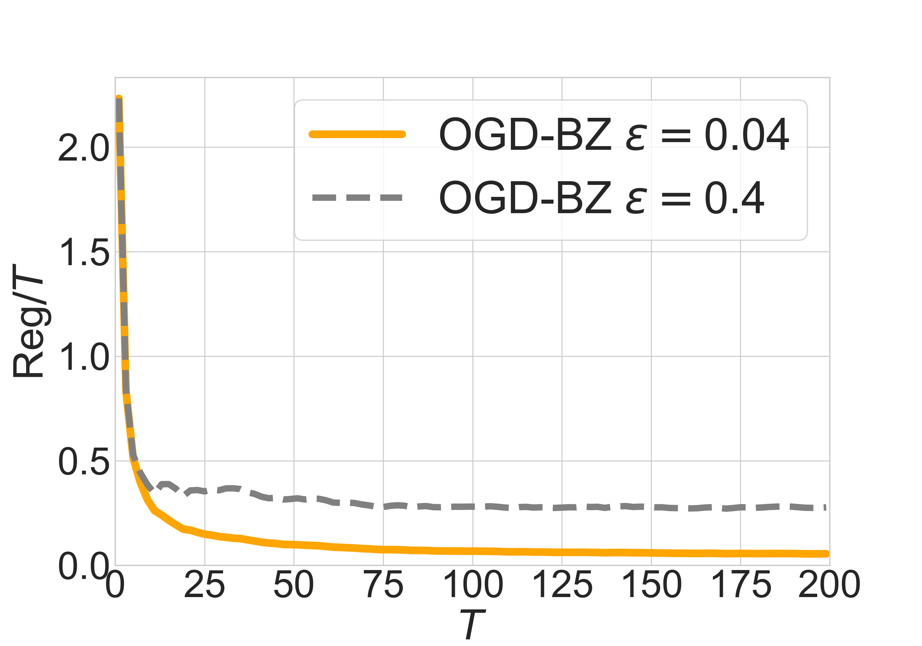
(a) Averaged regret

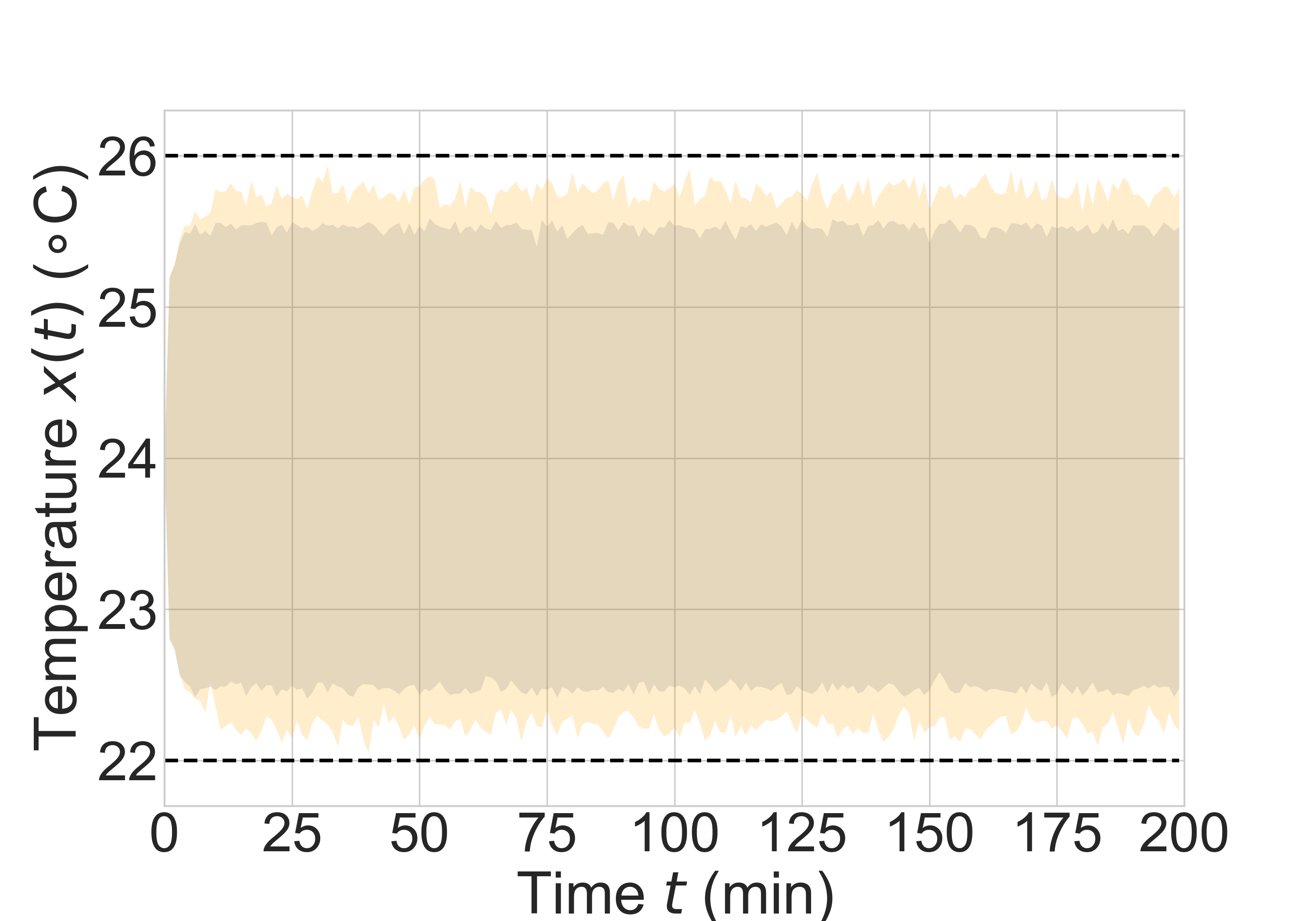
(b) $x(t)$’s range

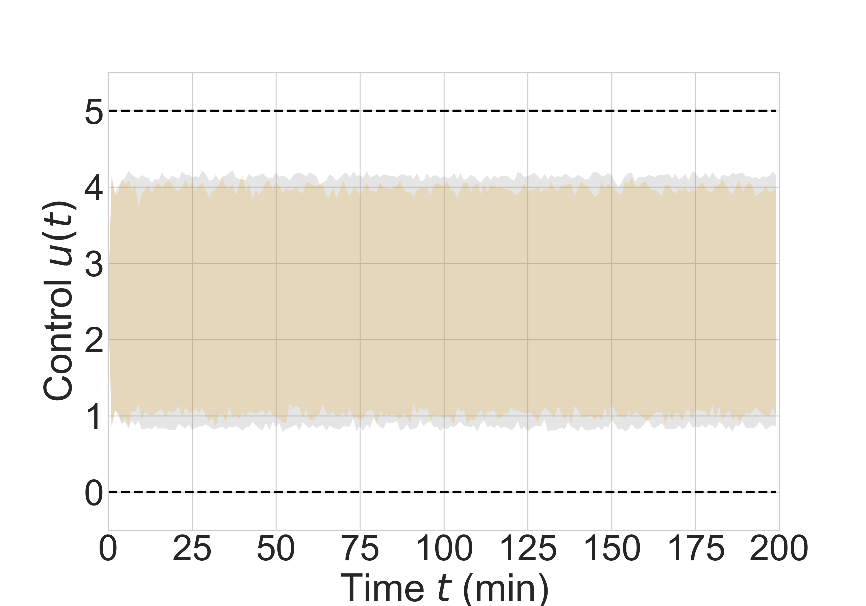
(c) $u(t)$’s range

Figure 1: Comparison of OGD-BZ with buffer sizes $\epsilon=0.04$ and $\epsilon=0.4$. In Figure (b) and (c), the yellow shade represents the range of $x(t)$ generated by OGD-BZ with $\epsilon=0.04$, while the grey shade is generated by OGD-BZ with $\epsilon=0.4$.

Figure 1 plots the comparison of OGD-BZ with different buffer sizes. Specifically, $\epsilon=0.04$ is a properly chosen buffer size and $\epsilon=0.4$ offers larger buffer zones. From Figure 1-(a), we can observe that the averaged regret with a properly chosen buffer size $\epsilon=0.04$ quickly diminishes to 0, which is consistent with Theorem 2. In addition, Figure 1-(b) and Figure 1-(c) plot the range of $x(t)$ and $u(t)$ under random disturbances in 1000 trials to demonstrate the safety of OGD-BZ. With a larger buffer zone, i.e. $\epsilon=0.4$, the range of $x_{t}$ is smaller and further from the boundaries, thus being safer. Interestingly, the range of $u(t)$ becomes slightly larger, which still satisfies the control constraints because the control constraints are not binding/active in this experiment and which indicates more control power is used here to ensure a smaller range of $x(t)$ under disturbances. Finally, the regret with $\epsilon=0.4$ is worse than that with $\epsilon=0.04$, which demonstrates the trade-off between safety and performance and how the choices of the buffer size affect this trade-off.

Supplementary Proofs for Lemma 7

Proof of Proposition 2

Since $\Omega_{2}\subseteq\Omega_{1}$, we have $\min_{\Omega_{2}}f(x)-\min_{\Omega_{1}}f(x)\geq 0$. Let $x_{1}^{*}=\operatorname*{arg\,min}_{\Omega_{1}}f(x)$. We will show that there exists $x_{2}^{\dagger}\in\Omega_{2}$ such that $\|x_{1}^{*}-x_{2}^{\dagger}\|_{2}\leq\frac{\delta_{1}\|\Delta\|_{\infty}}{\min_{i\in S}(h-C\mathring{x})_{i}}$, where $S=\{i:\Delta_{i}>0\}$. Then, by the Lipschitz continuity, we can prove the bound: $\min_{\Omega_{2}}f(x)\!-\!\min_{\Omega_{1}}f(x)\leq f(x_{2}^{\dagger})\!-\!f(x_{1}^{*})\!\leq\!\frac{L\delta_{1}\|\Delta\|_{\infty}}{\min_{i\in S}(h\!-\!C\mathring{x})_{i}}.$

In the following, we will show, more generally, that there exists $x_{2}\in\Omega_{2}$ that is close to $x_{1}$ for any $x_{1}\in\Omega_{1}$. For ease of notation, we define $y=x-\mathring{x}$, $\Omega_{1}^{y}=\{y:Cy\leq h-C\mathring{x}\}$, and $\Omega_{2}^{y}=\{y:Cy\leq h-C\mathring{x}-\Delta\}$. Notice that $0\in\Omega_{2}^{y}$ and $(h-C\mathring{x}-\Delta)_{i}\geq 0$. Besides, we have $y_{1}=x_{1}-\mathring{x}\in\Omega_{1}^{y}$. Further, by the convexity of $\Omega_{1}^{y}$, we have $\lambda y_{1}\in\Omega_{1}^{y}$ for $0\leq\lambda\leq 1$.

If $(Cy_{1})_{i}\leq(h-C\mathring{x}-\Delta)_{i}$ for all $i$, then $y_{1}\in\Omega_{2}^{y}$ and $x_{1}\in\Omega_{2}$. So we can let $x_{2}=x_{1}$ and $\|x_{2}-x_{1}\|_{2}=0$.

If, instead, there exists a set $S^{\prime}$ such that for any $i\in S^{\prime}$, $(Cy_{1})_{i}>(h-C\mathring{x}-\Delta)_{i}$. Then, define

$$\lambda=\min_{i\in S^{\prime}}\frac{(h-C\mathring{x}-\Delta)_{i}}{(Cy_{1})_{i}}.$$

Notice that $\lambda\in[0,1)$. We can show that $\lambda y_{1}\in\Omega_{2}^{y}$ below. When $i\in S^{\prime}$, $(\lambda Cy_{1})_{i}\leq(Cy_{1})_{i}\frac{(h-C\mathring{x}-\Delta)_{i}}{(Cy_{1})_{i}}=(h-C\mathring{x}-\Delta)_{i}$. When $i\not\in S^{\prime}$, we have $(\lambda Cy_{1})_{i}\leq\lambda(h-C\mathring{x}-\Delta)_{i}\leq(h-C\mathring{x}-\Delta)_{i}$. Therefore, $\lambda y_{1}\in\Omega_{2}^{y}$. Define $x_{2}=\lambda y_{1}+\mathring{x}$, then $x_{2}\in\Omega_{2}$. Notice that $\|x_{1}-x_{2}\|_{2}=\|y_{1}-y_{2}\|_{2}=(1-\lambda)\|y_{1}\|_{2}\leq(1-\lambda)\delta_{1}$. Since $y_{1}\in\Omega_{1}^{y}$, when $i\in S^{\prime}$, we have $0\leq(h-C\mathring{x}-\Delta)_{i}<(Cy_{1})_{i}\leq(h-C\mathring{x})_{i}$. Therefore, $\frac{(h-C\mathring{x}-\Delta)_{i}}{(Cy_{1})_{i}}\geq\frac{(h-C\mathring{x}-\Delta)_{i}}{(h-C\mathring{x})_{i}}=1-\frac{\Delta_{i}}{(h-C\mathring{x})_{i}}$. Consequently, by $S^{\prime}\subseteq S$, we have $1-\lambda\leq\max_{i\in S^{\prime}}\frac{\Delta_{i}}{(h-C\mathring{x})_{i}}\leq\frac{\|\Delta\|_{\infty}}{\min_{i\in S^{\prime}}(h-C\mathring{x})_{i}}\leq\frac{\|\Delta\|_{\infty}}{\min_{i\in S}(h-C\mathring{x})_{i}}.$

Proof of Lemma 9

We first provide an explicit expression for $\Gamma_{\epsilon}$ and then prove the bounds on $\Gamma_{\epsilon}$ based on the explicit expression.

Lemma 10.

For any $\epsilon\in\mathbb{R}$, $\bm{M}\in\Omega_{\epsilon}$ if and only if there exist $\{Y^{x}_{i,k,l}\}_{(1\leq i\leq k_{x},1\leq k\leq 2H,1\leq l\leq n)}$, $\{\!Y^{u}_{j,k,l}\!\}_{(1\leq j\leq k_{u},1\leq k\leq 2H,1\leq l\leq n)},\{\!Z^{[i]}_{k,j}\!\}_{(1\leq i\leq H,1\leq k\leq m,1\leq j\leq n)}$ such that

$$\begin{cases}&\sum_{k=1}^{2H}\sum_{l=1}^{n}Y^{x}_{i,k,l}\bar{w}\leq d_{x,i}-\epsilon,\ \forall 1\leq i\leq k_{x}\\ &\sum_{k=1}^{2H}\sum_{l=1}^{n}Y^{u}_{j,k,l}\bar{w}\leq d_{u,j}-\epsilon,\ \forall 1\leq j\leq k_{u}\\ &\sum_{j=1}^{n}Z^{[i]}_{k,j}\leq 2\sqrt{n}\kappa^{3}(1-\gamma)^{i-1},\forall 1\!\leq\!i\!\leq\!H,\!1\!\leq\!k\!\leq\!m\\ &-Y^{x}_{i,k,l}\leq(D_{x,i}^{\top}\mathring{\Phi}_{k}^{x}(\bm{M}))_{l}\leq Y^{x}_{i,k,l},\quad\forall i,k,l\\ &-Y^{u}_{j,k,l}\leq(D_{u,j}^{\top}\mathring{\Phi}_{k}^{u}(\bm{M}))_{l}\leq Y^{u}_{j,k,l}\quad\forall i,k,l\\ &-Z^{[i]}_{k,j}\leq M^{[i]}_{k,j}\leq Z^{[i]}_{k,j},\quad\forall i,k,j.\end{cases}$$

Let $\vec{W}$ denote the vector containing the elements of $\bm{M},\bm{Y}^{x}=\{Y^{x}_{i,k,l}\},\bm{Y}^{u}=\{Y^{u}_{j,k,l}\},\bm{Z}=\{Z^{[i]}_{k,j}\}$. Thus, the constraints above can be written as $\Gamma_{\epsilon}=\{\vec{W}:C\vec{W}\leq h_{\epsilon}\}.$

Since Lemma 10 holds for any $\epsilon\in\mathbb{R}$, we can similarly define $\Gamma_{-\epsilon_{1}-\epsilon_{3}}=\{\vec{W}:C\vec{W}\leq h_{-\epsilon_{1}-\epsilon_{3}}\}$ which is equivalent to $\Omega_{-\epsilon_{1}-\epsilon_{3}}$. Lemma 10 is based on a standard reformulation method in constrained optimization to handle inequalities involving absolute values so the proof is omitted.

Proof of (i). Firstly, notice that $\sum_{j=1}^{n}(M_{k,j}^{[i]})^{2}\leq\sum_{j=1}^{n}(Z_{k,j}^{[i]})^{2}\leq(\sum_{j=1}^{n}Z_{k,j}^{[i]})^{2}\leq 4n\kappa^{6}(1-\gamma)^{2i-2}$. Then,

$$\sum_{k=1}^{m}\sum_{i=1}^{H}\sum_{j=1}^{n}(M_{k,j}^{[i]})^{2}\leq\sum_{k=1}^{m}\sum_{i=1}^{H}\sum_{j=1}^{n}(Z_{k,j}^{[i]})^{2}\leq 4nm\kappa^{6}\frac{1}{2\gamma-\gamma^{2}}$$

Similarly, by the first two constraints in Lemma 10 and by the definition of $\Gamma_{-\epsilon_{1}-\epsilon_{3}}$, we have $\sum_{k=1}^{2H}\sum_{l=1}^{n}(Y^{x}_{i,k,l})^{2}\leq(d_{x,i}+\epsilon_{1}+\epsilon_{3})^{2}/\bar{w}^{2}\leq(d_{x,i}+\epsilon_{*})^{2}/\bar{w}^{2}$ and $\sum_{k=1}^{2H}\sum_{l=1}^{n}(Y^{u}_{j,k,l})^{2}\leq(d_{u,j}+\epsilon_{1}+\epsilon_{3})^{2}/\bar{w}^{2}\leq(d_{u,j}+\epsilon_{*})^{2}/\bar{w}^{2}$. Therefore, $\sum_{i=1}^{k_{x}}\sum_{k=1}^{2H}\sum_{l=1}^{n}(Y^{x}_{i,k,l})^{2}\leq\sum_{i=1}^{k_{x}}(d_{x,i}+\epsilon_{*})^{2}/\bar{w}^{2},$ and $\sum_{j=1}^{k_{u}}\sum_{k=1}^{2H}\sum_{l=1}^{n}(Y^{u}_{j,k,l})^{2}\leq\sum_{j=1}^{k_{u}}(d_{u,j}+\epsilon_{*})^{2}/\bar{w}^{2}$. Consequently,

$$\|\bm{M}\|_{F}^{2}+\|\bm{Y}^{x}\|_{F}^{2}+\|\bm{Y}^{u}\|_{F}^{2}+\|\bm{Z}\|_{F}^{2}$$

$$\leq\ \frac{8nm\kappa^{6}}{2\gamma-\gamma^{2}}+\frac{\sum_{i=1}^{k_{x}}(d_{x,i}+\epsilon_{*})^{2}+\sum_{j=1}^{k_{u}}(d_{u,j}+\epsilon_{*})^{2}}{\bar{w}^{2}}=\delta_{1}^{2}$$

where $\delta_{1}=\Theta(\sqrt{mn}+\sqrt{k_{c}})$ by the boundedness of $\epsilon_{*},d_{x},d_{u}$. (Although $\delta_{1}$ depends linearly on $1/\bar{w}$, we will show $L=TG_{f}$ and $G_{f}$ is quadratic on $\bar{w}$ by Lemma 5, hence, $L\delta_{1}$ is still linear with $\bar{w}$.)

Proof of (ii). Since the gradient of $\mathring{f}_{t}(\bm{M})$ is bounded by $G_{f}=\Theta(\sqrt{n^{3}mH^{3}})$, the gradient of $\sum_{t=0}^{T}\mathring{f}_{t}(\bm{M})$ is bounded by $LG_{f}=\Theta(T\sqrt{n^{3}mH^{3}})$.

Proof of (iii). Notice that the differences between $\Gamma_{\epsilon}$ and $\Gamma_{-\epsilon_{1}-\epsilon_{3}}$ come from the first two lines of the right-hand-side of inequalities in Lemma 10, which is $\epsilon+\epsilon_{1}+\epsilon_{3}$ in total.

Proof of (iv). From the proof of Theorem 1, we know that $\bm{M}(K_{*})\in\Omega_{\epsilon_{*}-\epsilon_{1}-\epsilon_{3}}\subseteq\Omega_{\epsilon}$. Therefore, there exist corresponding $\bm{Y}^{x}(K_{*}),\bm{Y}^{u}(K_{*}),\bm{Z}(K_{*})$ such that $\vec{W}^{\circ}=\text{vec}(\bm{M}(K_{*}),\bm{Y}^{x}(K_{*}),\bm{Y}^{u}(K_{*}),\bm{Z}(K_{*}))\in\Gamma_{\epsilon_{*}-\epsilon_{1}-\epsilon_{3}}\subseteq\Gamma_{\epsilon}$. Therefore, $\min_{\{i:\Delta_{i}>0\}}(h_{-\epsilon_{1}-\epsilon_{3}}\!-\!C\vec{W}^{\circ})_{i}\geq\epsilon_{1}+\epsilon_{3}-(-\epsilon_{*}+\epsilon_{1}+\epsilon_{3})=\epsilon_{*}$.

Conclusion and Future Work

This paper studies online optimal control with linear constraints and linear dynamics with random disturbances. We propose OGD-BZ and show that OGD-BZ can satisfy all the constraints despite disturbances and ensure $\tilde{O}(\sqrt{T})$ policy regret. There are many interesting future directions, e.g. (i) consider adversarial disturbances and robust stability, (ii) consider soft constraints and unbounded noises, (iii) consider bandit feedback, (iv) reduce the regret bound’s dependence on dimensions, (v) consider unknown systems, (vi) consider more general policies than linear policies, (vii) prove logarithmic regrets for strongly convex costs, etc.

Ethics Statement

The primary motivation for this paper is to develop an online control algorithm under linear constraints on the states and actions, and under noisy linear dynamics. Some practical physical systems can be approximated by noisy linear dynamics and most practical systems have to satisfy certain constraints on the states and actions, such as data center cooling and robotics, etc. Our proposed approach ensures to generate control policies that satisfy the constraints even under the uncertainty of unknown noises. Thus our algorithm can potentially be very beneficial for safety critical applications. However, note that our approach relies on a set of technical assumptions, as mentioned in the paper, which may not directly hold for all practical applications. Hence, when applying our algorithm, particular cares are needed when modeling the system and the constraints.

Appendix

In the following, we provide a complete proof for the technical results in the main submission. Specifically, Appendix A provides some helping lemmas, Appendix B provides proofs for Section 5.1, and Appendix C provides proofs for Section 5.2.

Helping lemmas

In this section, we provide some technical lemmas that will be useful in the proofs. These lemmas are similar to the results established in (Agarwal et al. 2019; Agarwal, Hazan, and Singh 2019) but involve slightly different coefficients in the bounds because we define $\mathcal{M}$ differently.

- A property of $(\kappa,\gamma)$ strongly stable matrices.

Lemma 11.

When $K$ is $(\kappa,\gamma)$ strongly stable, then $\|(A-BK)^{k}\|_{2}\leq\kappa^{2}(1-\gamma)^{k}$ for any integer $k\geq 0$.

Proof.

By Definition 2, there exist $H$ and $L$ such that $A-BK=H^{-1}LH$. Thus, $(A-BK)^{k}=H^{-1}L^{k}H$, and $\|(A-BK)^{k}\|_{2}\leq\|H^{-1}\|_{2}\|L^{k}\|_{2}\|H\|_{2}\leq\|H^{-1}\|_{2}\|L\|_{2}^{k}\|H\|_{2}\leq\kappa^{2}(1-\gamma)^{k}$ when $k\geq 1$. When $k=0$, $\|(A-BK)^{0}\|_{2}=\|I\|_{2}=1\leq\kappa^{2}$ since $\kappa\geq 1$. ∎

- A property of set $\mathcal{M}$.

Lemma 12.

For $\bm{M}\in\mathcal{M}=\{\bm{M}=\{M^{[1]},\dots,M^{[H]}\}:\ \|M^{[i]}\|_{\infty}\leq 2\sqrt{n}\kappa^{3}(1-\gamma)^{i-1}\}$, we have

$$\|M^{[i]}\|_{2}\leq 2\sqrt{mn}\kappa^{3}(1-\gamma)^{i-1}$$

Proof.

The proof is by $\|M^{[i]}\|_{2}\leq\sqrt{m}\|M^{[i]}\|_{\infty}$ due to properties of matrix norms. ∎

- Bounds on the states $x_{t}$, the actions $u_{t}$, the approximate states $\tilde{x}_{t}$, and the approximate actions $\tilde{u}_{t}$.

Lemma 13.

For $\bm{M}_{0},\dots,\bm{M}_{T}\in\mathcal{M}$, we have

$$\|\Phi^{x}_{k}(\bm{M}_{t-H:t-1})\|_{2}\leq\kappa^{2}(1-\gamma)^{k-1}\mathds{1}_{(k\leq H)}+\phi H(1-\gamma)^{k-2}\mathds{1}_{(k\geq 2)}$$

$$\|\Phi^{u}_{k}(\bm{M}_{t-H:t})\|_{2}\leq\kappa^{3}(1-\gamma)^{k-1}\mathds{1}_{(k\leq H)}(2\sqrt{nm}+1)+\kappa\phi H(1-\gamma)^{k-2}\mathds{1}_{(k\geq 2)}$$

where $\phi=2\kappa^{5}\kappa_{B}\sqrt{mn}$.

Proof.

By Proposition 1, Lemma 11, the definition of $\mathcal{M}$, and Definition 4, we have

$$\|\Phi_{k}^{x}(\bm{M}_{t-H:t-1})\|_{2} =\|A_{\mathbb{K}}^{k-1}\mathds{1}_{(k\leq H)}+\sum_{i=1}^{H}A_{\mathbb{K}}^{i-1}BM_{t-i}^{[k-i]}\mathds{1}_{(1\leq k-i\leq H)}\|$$

$$\leq\|A_{\mathbb{K}}^{k-1}\|_{2}\mathds{1}_{(k\leq H)}+\sum_{i=1}^{H}\|A_{\mathbb{K}}^{i-1}\|_{2}\|B\|_{2}\|M_{t-i}^{[k-i]}\|_{2}\mathds{1}_{(1\leq k-i\leq H)}$$

$$\leq\kappa^{2}(1-\gamma)^{k-1}\mathds{1}_{(k\leq H)}+\sum_{i=1}^{H}\kappa^{2}(1-\gamma)^{i-1}\kappa_{B}\sqrt{m}\|M_{t-i}^{[k-i]}\|_{\infty}\mathds{1}_{(1\leq k-i\leq H)}$$

$$\leq\kappa^{2}(1-\gamma)^{k-1}\mathds{1}_{(k\leq H)}+2\kappa^{5}\kappa_{B}\sqrt{mn}\sum_{i=1}^{H}(1-\gamma)^{i-1}(1-\gamma)^{k-i-1}\mathds{1}_{(1\leq k-i\leq H)}$$

$$\leq\kappa^{2}(1-\gamma)^{k-1}\mathds{1}_{(k\leq H)}+2\kappa^{5}\kappa_{B}\sqrt{mn}H(1-\gamma)^{k-2}\mathds{1}_{(k\geq 2)}$$

$$=\kappa^{2}(1-\gamma)^{k-1}\mathds{1}_{(k\leq H)}+\phi H(1-\gamma)^{k-2}\mathds{1}_{(k\geq 2)},$$

where $\phi=2\kappa^{5}\kappa_{B}\sqrt{mn}$.

Further, by Proposition 1, Lemma 11, the definition of $\mathcal{M}$, Definition 4, and the bound above, we have

$$\|\Phi_{k}^{u}(\bm{M}_{t-H:t})\|_{2} =\|M_{t}^{[k]}\mathds{1}_{(k\leq H)}-\mathbb{K}\Phi_{k}^{x}(\bm{M}_{t-H:t-1})\|_{2}$$

$$\leq\|M_{t}^{[k]}\|_{2}\mathds{1}_{(k\leq H)}+\|\mathbb{K}\|_{2}\|\Phi_{k}^{x}(\bm{M}_{t-H:t-1})\|_{2}$$

$$\leq\sqrt{m}\|M_{t}^{[k]}\|_{\infty}\mathds{1}_{(k\leq H)}+\|\mathbb{K}\|_{2}\|\Phi_{k}^{x}(\bm{M}_{t-H:t-1})\|_{2}$$

$$\leq 2\sqrt{nm}\kappa^{3}(1-\gamma)^{k-1}\mathds{1}_{(k\leq H)}+\kappa\left(\kappa^{2}(1-\gamma)^{k-1}\mathds{1}_{(k\leq H)}+\phi H(1-\gamma)^{k-2}\mathds{1}_{(k\geq 2)}\right)$$

$$=\kappa^{3}(1-\gamma)^{k-1}\mathds{1}_{(k\leq H)}(2\sqrt{nm}+1)+\kappa\phi H(1-\gamma)^{k-2}\mathds{1}_{(k\geq 2)}$$

∎

Lemma 14.

When implementing $\bm{M}_{0},\dots,\bm{M}_{T}\in\mathcal{M}$, we have

$$\max(\|x_{t}\|_{2},\|\tilde{x}_{2}\|_{2})\leq b_{x},\quad\max(\|u_{t}\|_{2},\|\tilde{u}_{2}\|_{2})\leq b_{u}$$

where $b_{x}\coloneqq\frac{\sqrt{n}\bar{w}(\kappa^{2}+\phi H)}{(1-\kappa^{2}(1-\gamma)^{H})\gamma}$ and $b_{u}=\kappa b_{x}+2\sqrt{mn}\kappa^{3}\bar{w}/\gamma$. Define $b=\max(b_{x},b_{u})=\frac{\kappa\sqrt{n}\bar{w}(\kappa^{2}+\phi H)}{(1-\kappa^{2}(1-\gamma)^{H})\gamma}+2\sqrt{mn}\kappa^{3}\bar{w}/\gamma$.

Consequently, when $H\geq\frac{\log(2\kappa^{2})}{\log((1-\gamma)^{-1})}$, we have $b\leq 8\sqrt{mn^{2}}H\bar{w}\kappa^{6}\kappa_{B}/\gamma$.

Proof.

Firstly, we bound $\|\tilde{x}_{t}\|_{2}$ below.

$$\|\tilde{x}_{t}\|_{2} =\|\sum_{k=1}^{2H}\Phi^{x}_{k}(\bm{M}_{t-H:t-1})w_{t-k}\|_{2}\leq\sum_{k=1}^{2H}\|\Phi^{x}_{k}(\bm{M}_{t-H:t-1})\|_{2}\sqrt{n}\bar{w}$$

$$\leq\sqrt{n}\bar{w}\sum_{k=1}^{2H}\left(\kappa^{2}(1-\gamma)^{k-1}\mathds{1}_{(k\leq H)}+\phi H(1-\gamma)^{k-2}\mathds{1}_{(k\geq 2)}\right)$$

$$\leq\sqrt{n}\bar{w}(\kappa^{2}/\gamma+\phi H/\gamma)\leq b_{x}$$

Next, we bound $\|x_{t}\|_{2}$ by $\|\tilde{x}_{t}\|_{2}$’s bound and induction based on the recursive equation in Proposition 1. Specifically, we first note that $\|x_{t-H}\|_{2}=0\leq b_{x}$ when $t=0$. At any $t\geq 0$, suppose $\|x_{t-H}\|_{2}\leq b_{x}$, then

$$\|x_{t}\|_{2} =\|A_{\mathbb{K}}^{H}x_{t-H}+\tilde{x}_{t}\|_{2}\leq\kappa^{2}(1-\gamma)^{H}b_{x}+\sqrt{n}\bar{w}(\kappa^{2}/\gamma+\phi H/\gamma)=b_{x}$$

Consequently, we have proved that $\|x_{t}\|_{2}\leq b_{x}$ for all $t$.

Similarly, we bound $\|\tilde{u}_{t}\|_{2}$ and $\|u_{t}\|_{2}$ below.

$$\|\tilde{u}_{t}\|_{2} =\left\|-\mathbb{K}\tilde{x}_{t}+\sum_{i=1}^{H}M_{t}^{[i]}w_{t-i}\right\|_{2}\leq\|-\mathbb{K}\tilde{x}_{t}\|_{2}+\sum_{i=1}^{H}\|M_{t}^{[i]}w_{t-i}\|_{2}$$

$$\leq\|-\mathbb{K}\tilde{x}_{t}\|_{2}+\sum_{i=1}^{H}\sqrt{m}\|M_{t}^{[i]}w_{t-i}\|_{\infty}$$

$$\leq\kappa b_{x}+\sum_{i=1}^{H}\sqrt{m}(2\sqrt{n})\kappa^{3}(1-\gamma)^{i-1}\bar{w}=\kappa b_{x}+2\sqrt{mn}\kappa^{3}\bar{w}/\gamma=b_{u}$$

Further, by Proposition 1, we have

$$\|u_{t}\|_{2} =\left\|-\mathbb{K}x_{t}+\sum_{i=1}^{H}M_{t}^{[i]}w_{t-i}\right\|_{2}\leq\|-\mathbb{K}x_{t}\|+\sum_{i=1}^{H}\sqrt{m}\|M_{t}^{[i]}w_{t-i}\|_{\infty}$$

$$\leq\kappa b_{x}+\sum_{i=1}^{H}2\sqrt{mn}\kappa^{3}(1-\gamma)^{i-1}\bar{w}$$

$$\leq\kappa b_{x}+2\sqrt{mn}\kappa^{3}\bar{w}/\gamma=b_{u}$$

Finally, notice that when $H\geq\frac{\log(2\kappa^{2})}{\log((1-\gamma)^{-1})}$, we have $\kappa^{2}(1-\gamma)^{H}\leq 1/2$, and thus $b_{x}\leq 2\sqrt{n}\bar{w}(\kappa^{2}+\phi H)/\gamma$ and $b$’s bound follows naturally.

∎

- Properties of $f_{t}(\bm{M}_{t-H:t})$ and $\mathring{f}_{t}(\bm{M}_{t})$

Lemma 15.

Consider any $\bm{M}_{t}\in\mathcal{M}$ and any $\tilde{\bm{M}_{t}}\in\mathcal{M}$ for all $t$, then

$$|f_{t}(\bm{M}_{t-H:t})-f_{t}(\tilde{\bm{M}}_{t-H:t})|\leq Gb(1+\kappa)\sqrt{n}\bar{w}\kappa^{2}\kappa_{B}\sum_{i=0}^{H}(1-\gamma)^{\max(i-1,0)}\sum_{j=1}^{H}\|M^{[j]}_{t-i}-\tilde{M}^{[j]}_{t-i}\|_{2}.$$

Further, $\|\nabla\mathring{f}_{t}(\bm{M}_{t})\|_{F}\leq G_{f}$ for $\bm{M}_{t}\in\mathcal{M}$, where $G_{f}=\Theta(Gb(1+\kappa)\sqrt{n}\bar{w}\kappa^{2}\kappa_{B}\sqrt{H}\frac{1+\gamma}{\gamma})$.

Consequently, when $H\geq\frac{\log(2\kappa^{2})}{\log((1-\gamma)^{-1})}$, then $G_{f}\leq\Theta(\sqrt{n^{3}H^{3}m})$.

Proof.

Let $\tilde{x}_{t}$ and $\accentset{\approx}{x}_{t}$ denote the approximate states generated by $\bm{M}_{t-H:t-1}$ and $\tilde{\bm{M}}_{t-H:t-1}$ respectively. Define $\tilde{u}_{t}$ and $\accentset{\approx}{u}_{t}$ similarly. We have

$$\|\tilde{x}_{t}-\accentset{\approx}{x}_{t}\|_{2} =\|\sum_{k=1}^{2H}(\Phi_{k}^{x}(\bm{M}_{t-H:t-1})-\Phi_{k}^{x}(\tilde{\bm{M}}_{t-H:t-1}))w_{t-k}\|_{2}$$

$$\leq\sum_{k=1}^{2H}\|\Phi_{k}^{x}(\bm{M}_{t-H:t-1})-\Phi_{k}^{x}(\tilde{\bm{M}}_{t-H:t-1})\|_{2}\sqrt{n}\bar{w}$$

$$\leq\sqrt{n}\bar{w}\sum_{k=1}^{2H}\|\sum_{i=1}^{H}A_{\mathbb{K}}^{i-1}B(M_{t-i}^{[k-i]}-\tilde{M}_{t-i}^{[k-i]})\mathds{1}_{(1\leq k-i\leq H)}\|_{2}$$

$$\leq\sqrt{n}\bar{w}\sum_{k=1}^{2H}\sum_{i=1}^{H}\kappa^{2}(1-\gamma)^{i-1}\kappa_{B}\|M_{t-i}^{[k-i]}-\tilde{M}_{t-i}^{[k-i]}\|_{2}\mathds{1}_{(1\leq k-i\leq H)}$$

$$=\sqrt{n}\bar{w}\kappa^{2}\kappa_{B}\sum_{i=1}^{H}(1-\gamma)^{i-1}\sum_{j=1}^{H}\|M_{t-i}^{[j]}-\tilde{M}_{t-i}^{[j]}\|_{2}$$

and

$$\|\tilde{u}_{t}-\accentset{\approx}{u}_{t}\|_{2} =\|-\mathbb{K}\tilde{x}_{t}+\mathbb{K}\accentset{\approx}{x}_{t}+\sum_{i=1}^{H}M_{t}^{[i]}w_{t-i}-\sum_{i=1}^{H}\tilde{M}_{t}^{[i]}w_{t-i}\|_{2}$$

$$\leq\kappa\|\tilde{x}_{t}-\accentset{\approx}{x}_{t}\|_{2}+\sqrt{n}\bar{w}\sum_{i=1}^{H}\|M_{t}^{[i]}-\tilde{M}_{t}^{[i]}\|_{2}$$

$$\leq\sqrt{n}\bar{w}\kappa^{3}\kappa_{B}\sum_{i=0}^{H}(1-\gamma)^{\max(i-1,0)}\sum_{j=1}^{H}\|M^{[j]}_{t-i}-\tilde{M}^{[j]}_{t-i}\|_{2}$$

Consequently, by Assumption 2 and Lemma 14, we can prove the first bound in the lemma’s statement below.

$$|f_{t}(\bm{M}_{t-H:t-1})-f_{t}(\tilde{\bm{M}}_{t-H:t-1})| =|c_{t}(\tilde{x}_{t},\tilde{u}_{t})-c_{t}(\accentset{\approx}{x}_{t},\accentset{\approx}{u}_{t})|$$

$$\leq Gb(\|\tilde{x}_{t}-\accentset{\approx}{x}_{t}\|_{2}+\|\tilde{u}_{t}-\accentset{\approx}{u}_{t}\|_{2})$$

$$\leq Gb(1+\kappa)\sqrt{n}\bar{w}\kappa^{2}\kappa_{B}\sum_{i=0}^{H}(1-\gamma)^{\max(i-1,0)}\sum_{j=1}^{H}\|M^{[j]}_{t-i}-\tilde{M}^{[j]}_{t-i}\|_{2}.$$

Next, we prove the gradient bound on $\mathring{f}_{t}(\bm{M}_{t})$. Define a set $\mathcal{M}_{out,H}=\{\bm{M}:\|M[k]\|_{\infty}\leq 4\kappa^{2}\sqrt{n}(1-\gamma)^{k-1}\}$, whose interior contains $\mathcal{M}_{H}$. Similar to Lemma 15, we can show $\mathring{f}_{t}(\bm{M}+\Delta\bm{M})-\mathring{f}_{t}(\bm{M})\leq\Theta(b\sqrt{n}w_{\max}\sum_{i=0}^{H}(1-\gamma)^{\max(i-1,0)}\sum_{j=1}^{H}\|\Delta M{[j]}\|_{2})$ for any $\bm{M}\in\mathcal{M}_{H}$ and $\bm{M}+\Delta\bm{M}+\mathcal{M}_{out,H}$.

By the definition of the operator’s norm, we have

$$\|\nabla\mathring{f}_{t}(\bm{M})\|_{F}=\sup_{\Delta\bm{M}\not=0,\bm{M}+\Delta\bm{M}+\mathcal{M}_{out,H}}\frac{\langle\nabla\mathring{f}_{t}(\bm{M}),\Delta\bm{M}\rangle}{\|\Delta\bm{M}\|_{F}}$$

$$\leq\sup_{\Delta\bm{M}\not=0,\bm{M}+\Delta\bm{M}+\mathcal{M}_{out,H}}\frac{\mathring{f}_{t}(\bm{M}+\Delta\bm{M})-\mathring{f}_{t}(\bm{M})}{\|\Delta\bm{M}\|_{F}}$$

$$\leq\sup_{\Delta\bm{M}\not=0,\bm{M}+\Delta\bm{M}+\mathcal{M}_{out,H}}\frac{\Theta(b\sqrt{n}w_{\max}\sum_{i=0}^{H}(1-\gamma)^{\max(i-1,0)}\sum_{j=1}^{H}\|\Delta M^{[j]}\|_{2})}{\|\Delta\bm{M}\|_{F}}$$

$$\leq\sup_{\Delta\bm{M}\not=0,\bm{M}+\Delta\bm{M}+\mathcal{M}_{out,H}}\frac{\Theta(b\sqrt{n}w_{\max}\sum_{i=0}^{H}(1-\gamma)^{\max(i-1,0)}\sqrt{H}\|\Delta\bm{M}\|_{F})}{\|\Delta\bm{M}\|_{F}}$$

$$\leq\Theta(b\sqrt{n}w_{\max}\sqrt{H}\frac{1+\gamma}{\gamma})$$

∎

Proofs of the lemmas used in the proof of Theorem 1

Proof of Lemma 1

The proof is straightforward from Lemma 11 and Lemma 14.

$$\|D_{x}A_{\mathbb{K}}^{H}x_{t-H}\|_{\infty} \leq\|D_{x}\|_{\infty}\|A_{\mathbb{K}}^{H}x_{t-H}\|_{\infty}\leq\|D_{x}\|_{\infty}\|A_{\mathbb{K}}^{H}x_{t-H}\|_{2}$$

$$\leq\|D_{x}\|_{\infty}\|A_{\mathbb{K}}^{H}\|_{2}\|x_{t-H}\|_{2}\leq\|D_{x}\|_{\infty}\kappa^{2}(1-\gamma)^{H}b\leq\epsilon_{1}(H)$$

$$\|D_{u}\mathbb{K}A_{\mathbb{K}}^{H}x_{t-H}\|_{\infty} \leq\|D_{u}\|_{\infty}\|\mathbb{K}A_{\mathbb{K}}^{H}x_{t-H}\|_{\infty}\leq\|D_{u}\|_{\infty}\|\mathbb{K}A_{\mathbb{K}}^{H}x_{t-H}\|_{2}$$

$$\leq\|D_{u}\|_{\infty}\|\mathbb{K}\|_{2}\|A_{\mathbb{K}}^{H}\|_{2}\|x_{t-H}\|_{2}\leq\|D_{u}\|_{\infty}\kappa^{3}(1-\gamma)^{H}b\leq\epsilon_{1}(H)$$

Hence, we have $\epsilon_{1}(H)=c_{1}n\sqrt{m}H(1-\gamma)^{H}$ and $c_{1}=8\bar{w}\kappa^{9}\kappa_{B}\max(\|D_{x}\|_{\infty},\|D_{u}\|_{\infty})/\gamma$.

Proof of Lemma 3

Lemma 3 is proved by first establishing a smoothness property of $g_{i}^{x}(\cdot)$ and $g_{j}^{u}(\cdot)$ in Lemma 16 and then leveraging the slow updates of OGD. The details of the proof are provided below.

Lemma 16.

Consider any $\bm{M}_{t}\in\mathcal{M}$ and any $\tilde{\bm{M}_{t}}\in\mathcal{M}$ for all $t$, then

$$\max_{1\leq i\leq k_{x}}\left|g^{x}_{i}(\bm{M}_{t-H:t-1})-g^{x}_{i}(\tilde{\bm{M}}_{t-H:t-1})\right|\leq L_{g}(H)\sum_{k=1}^{H}(1-\gamma)^{k-1}\|\bm{M}_{t-k}-\tilde{\bm{M}}_{t-k}\|_{F}$$

$$\max_{1\leq j\leq k_{u}}\left|g^{u}_{j}(\bm{M}_{t-H:t})-g^{u}_{j}(\tilde{\bm{M}}_{t-H:t})\right|\leq L_{g}(H)\sum_{k=0}^{H}(1-\gamma)^{\max(k-1,0)}\|\bm{M}_{t-k}-\tilde{\bm{M}}_{t-k}\|_{F}$$

where $L_{g}(H)=\bar{w}\sqrt{n}\max(\|D_{x}\|_{\infty},\|D_{u}\|_{\infty})\kappa^{3}\kappa_{B}\sqrt{H}.$

Proof.

We first provide a bound on $\|D_{x,i}^{\top}\Phi^{x}_{k}(\bm{M}_{t-H:t-1})\|_{1}-\|D_{x,i}^{\top}\Phi^{x}_{k}(\tilde{\bm{M}}_{t-H:t-1})\|_{1}$.

$$|\|D_{x,i}^{\top}\Phi^{x}_{k}(\bm{M}_{t-H:t-1})\|_{1}-\|D_{x,i}^{\top}\Phi^{x}_{k}(\tilde{\bm{M}}_{t-H:t-1})\|_{1}|\leq\|D_{x,i}^{\top}\Phi^{x}_{k}(\bm{M}_{t-H:t-1})-D_{x,i}^{\top}\Phi^{x}_{k}(\tilde{\bm{M}}_{t-H:t-1})\|_{1}$$

$$=\ \left\|D_{x,i}^{\top}\left(\sum_{s=1}^{H}A_{\mathbb{K}}^{s-1}B(M_{t-s}^{[k-s]}-\tilde{M}_{t-s}^{[k-s]})\mathds{1}_{(1\leq k-s\leq H)}\right)\right\|_{1}$$

$$=\ \left\|\sum_{s=1}^{H}D_{x,i}^{\top}A_{\mathbb{K}}^{s-1}B(M_{t-s}^{[k-s]}-\tilde{M}_{t-s}^{[k-s]})\mathds{1}_{(1\leq k-s\leq H)}\right\|_{1}$$

$$\leq\ \sqrt{n}\left\|\sum_{s=1}^{H}D_{x,i}^{\top}A_{\mathbb{K}}^{s-1}B(M_{t-s}^{[k-s]}-\tilde{M}_{t-s}^{[k-s]})\mathds{1}_{(1\leq k-s\leq H)}\right\|_{2}$$

$$\leq\ \sqrt{n}\sum_{s=1}^{H}\|D_{x,i}^{\top}\|_{2}\|A_{\mathbb{K}}^{s-1}\|_{2}\|B\|_{2}\|M_{t-s}^{[k-s]}-\tilde{M}_{t-s}^{[k-s]}\|_{2}\mathds{1}_{(1\leq k-s\leq H)}$$

$$\leq\ \sqrt{n}\sum_{s=1}^{H}\|D_{x,i}^{\top}\|_{1}\kappa^{2}(1-\gamma)^{s-1}\kappa_{B}\|M_{t-s}^{[k-s]}-\tilde{M}_{t-s}^{[k-s]}\|_{2}\mathds{1}_{(1\leq k-s\leq H)}$$

$$\leq\ \sqrt{n}\|D_{x}\|_{\infty}\kappa^{2}\kappa_{B}\sum_{s=1}^{H}(1-\gamma)^{s-1}\|M_{t-s}^{[k-s]}-\tilde{M}_{t-s}^{[k-s]}\|_{2}\mathds{1}_{(1\leq k-s\leq H)}$$

Therefore, for any $1\leq i\leq k_{x}$, we have

$$\quad\ |g^{x}_{i}(\bm{M}_{t-H:t-1})-g^{x}_{i}(\tilde{\bm{M}}_{t-H:t-1})|$$

$$\leq\bar{w}\sum_{k=1}^{2H}|\|D_{x,i}^{\top}\Phi^{x}_{k}(\bm{M}_{t-H:t-1})\|_{1}-\|D_{x,i}^{\top}\Phi^{x}_{k}(\tilde{\bm{M}}_{t-H:t-1})\|_{1}|$$

$$\leq\bar{w}\sqrt{n}\|D_{x}\|_{\infty}\kappa^{2}\kappa_{B}\sum_{k=1}^{2H}\sum_{s=1}^{H}(1-\gamma)^{s-1}\|M_{t-s}^{[k-s]}-\tilde{M}_{t-s}^{[k-s]}\|_{2}\mathds{1}_{(1\leq k-s\leq H)}$$

$$=\bar{w}\sqrt{n}\|D_{x}\|_{\infty}\kappa^{2}\kappa_{B}\sum_{s=1}^{H}\sum_{k=1}^{2H}(1-\gamma)^{s-1}\|M_{t-s}^{[k-s]}-\tilde{M}_{t-s}^{[k-s]}\|_{2}\mathds{1}_{(1\leq k-s\leq H)}$$

$$\leq\bar{w}\sqrt{n}\|D_{x}\|_{\infty}\kappa^{2}\kappa_{B}\sum_{s=1}^{H}\sum_{k=1}^{2H}(1-\gamma)^{s-1}\|M_{t-s}^{[k-s]}-\tilde{M}_{t-s}^{[k-s]}\|_{F}\mathds{1}_{(1\leq k-s\leq H)}$$

$$\leq\bar{w}\sqrt{n}\|D_{x}\|_{\infty}\kappa^{2}\kappa_{B}\sqrt{H}\sum_{s=1}^{H}(1-\gamma)^{s-1}\|\bm{M}_{t-s}-\tilde{\bm{M}}_{t-s}\|_{F}$$

Next, we provide a bound on $\|D_{u,j}^{\top}\Phi^{u}_{k}(\bm{M}_{t-H:t})\|_{1}-\|D_{u,j}^{\top}\Phi^{u}_{k}(\tilde{\bm{M}}_{t-H:t})\|_{1}$.

$$|\|D_{u,j}^{\top}\Phi^{u}_{k}(\bm{M}_{t-H:t})\|_{1}-\|D_{u,j}^{\top}\Phi^{u}_{k}(\tilde{\bm{M}}_{t-H:t})\|_{1}|\leq\|D_{u,j}^{\top}(\Phi^{u}_{k}(\bm{M}_{t-H:t})-\Phi^{u}_{k}(\tilde{\bm{M}}_{t-H:t})\|_{1}$$

$$\leq\ \|D_{u,j}^{\top}(M_{t}^{[k]}-\tilde{M}_{t}^{[k]})\|_{1}\mathds{1}_{(k\leq H)}+\left\|\sum_{s=1}^{H}D_{u,j}^{\top}\mathbb{K}A_{\mathbb{K}}^{s-1}B(M_{t-s}^{[k-s]}-\tilde{M}_{t-s}^{[k-s]})\right\|_{1}\mathds{1}_{(1\leq k-s\leq H)}$$

$$\leq\ \sqrt{n}\|D_{u,j}^{\top}(M_{t}^{[k]}-\tilde{M}_{t}^{[k]})\|_{2}\mathds{1}_{(k\leq H)}+\sqrt{n}\left\|\sum_{s=1}^{H}D_{u,j}^{\top}\mathbb{K}A_{\mathbb{K}}^{s-1}B(M_{t-s}^{[k-s]}-\tilde{M}_{t-s}^{[k-s]})\right\|_{2}\mathds{1}_{(1\leq k-s\leq H)}$$

$$\leq\ \sqrt{n}\|D_{u,j}^{\top}\|_{2}\|M_{t}^{[k]}-\tilde{M}_{t}^{[k]}\|_{2}\mathds{1}_{(k\leq H)}+\sqrt{n}\sum_{s=1}^{H}\|D_{u,j}\|_{2}\kappa^{3}(1-\gamma)^{s-1}\kappa_{B}\|M_{t-s}^{[k-s]}-\tilde{M}_{t-s}^{[k-s]}\|_{2}\mathds{1}_{(1\leq k-s\leq H)}$$

$$\leq\ \sqrt{n}\|D_{u,j}^{\top}\|_{1}\|M_{t}^{[k]}-\tilde{M}_{t}^{[k]}\|_{2}\mathds{1}_{(k\leq H)}+\sqrt{n}\sum_{s=1}^{H}\|D_{u,j}\|_{1}\kappa^{3}(1-\gamma)^{s-1}\kappa_{B}\|M_{t-s}^{[k-s]}-\tilde{M}_{t-s}^{[k-s]}\|_{2}\mathds{1}_{(1\leq k-s\leq H)}$$

Therefore, for any $1\leq j\leq k_{u}$, we have

$$\quad\ |g^{u}_{j}(\bm{M}_{t-H:t})-g^{u}_{j}(\tilde{\bm{M}}_{t-H:t})|\leq\sum_{k=1}^{2H}\bar{w}|\|D_{u,j}^{\top}\Phi^{u}_{k}(\bm{M}_{t-H:t})\|_{1}-\|D_{u,j}^{\top}\Phi^{u}_{k}(\tilde{\bm{M}}_{t-H:t})\|_{1}|$$

$$\leq\bar{w}\sqrt{n}\|D_{u}\|_{\infty}\sqrt{H}\|\bm{M}_{t}-\tilde{\bm{M}}_{t}\|_{F}+\bar{w}\sqrt{n}\|D_{u}\|_{\infty}\kappa^{3}\kappa_{B}\sqrt{H}\sum_{s=1}^{H}(1-\gamma)^{s-1}\|\bm{M}_{t-s}-\tilde{\bm{M}}_{t-s}\|_{F}$$

$$\leq\bar{w}\sqrt{n}\|D_{u}\|_{\infty}\kappa^{3}\kappa_{B}\sqrt{H}\sum_{s=0}^{H}(1-\gamma)^{\max(s-1,0)}\|\bm{M}_{t-s}-\tilde{\bm{M}}_{t-s}\|_{F}$$

where the last inequality uses $\kappa\geq 1,\kappa_{B}\geq 1$. ∎

Proof of Lemma 3.

Firstly, by OGD’s definition and Lemma 15, we have $\|\bm{M}_{t}-\bm{M}_{t-1}\|_{F}\leq\eta G_{f}$ and $\|\bm{M}_{t}-\bm{M}_{t-k}\|_{F}\leq k\eta G_{f}$. By Lemma 16, we have

$$\max_{1\leq i\leq k_{x}}\left|g^{x}_{i}(\bm{M}_{t-H+1:t})-g^{x}_{i}({\bm{M}}_{t},\dots,\bm{M}_{t})\right|\leq L_{g}(H)\sum_{k=1}^{H-1}(1-\gamma)^{k-1}\|\bm{M}_{t-k}-\bm{M}_{t}\|_{F}$$

$$\leq L_{g}(H)\sum_{k=1}^{H-1}(1-\gamma)^{k-1}k\eta G_{f}\leq L_{g}(H)\eta G_{f}\frac{1}{\gamma^{2}}$$

and

$$\max_{1\leq j\leq k_{u}}\left|g^{u}_{j}(\bm{M}_{t-H:t})-g^{u}_{j}(\tilde{\bm{M}}_{t},\dots,\bm{M}_{t})\right|\leq L_{g}(H)\sum_{k=1}^{H}(1-\gamma)^{k-1}\|\bm{M}_{t-k}-\bm{M}_{t}\|_{F}\leq\epsilon_{2}(\eta,H)$$

$$\leq L_{g}(H)\sum_{k=1}^{H}(1-\gamma)^{k-1}k\eta G_{f}\leq L_{g}(H)\eta G_{f}\frac{1}{\gamma^{2}}\leq\epsilon_{2}(\eta,H)$$

where $\epsilon_{2}(\eta,H)=c_{2}n^{2}\sqrt{m}H^{2}\eta$. ∎

Proof of Lemma 4

Firstly, notice that when implementing $u_{t}^{K}=-Kx_{t}^{K}$ and $x_{0}=0$, we have

$$x_{t}^{K} =\sum_{s=1}^{t}A_{K}^{s-1}w_{t-s},\qquad u_{t}^{K}=-\sum_{s=1}^{t}KA_{K}^{s-1}w_{t-s},$$

where $A_{K}=A-BK$.

In addition, when implementing a disturbance-action controller $\bm{M}$, the state satisfies

$$x_{t}^{\bm{M}(K)} =\sum_{s=1}^{t}\tilde{\Phi}^{x}_{t,s}(\bm{M}(K))w_{t-s},\quad\text{ where }\tilde{\Phi}^{x}_{s}(\bm{M}(K))=A_{\mathbb{K}}^{s-1}+\sum_{j=\max(1,s-H)}^{s-1}A_{\mathbb{K}}^{j-1}BM^{[s-j]}(K).$$

Specifically, when $s\leq H$, we have

$$\tilde{\Phi}^{x}_{s}(\bm{M}(K)) =A_{\mathbb{K}}^{s-1}+\sum_{j=1}^{s-1}A_{\mathbb{K}}^{j-1}BM^{[s-j]}(K)$$

$$=A_{\mathbb{K}}^{s-1}+\sum_{j=1}^{s-1}A_{\mathbb{K}}^{j-1}B(\mathbb{K}-K)A_{K}^{s-j-1}$$

$$=A_{\mathbb{K}}^{s-1}+\sum_{j=1}^{s-1}A_{\mathbb{K}}^{j-1}(A_{K}-A_{\mathbb{K}})A_{K}^{s-j-1}$$

$$=A_{\mathbb{K}}^{s-1}+\sum_{j=1}^{s-1}A_{\mathbb{K}}^{j-1}A_{K}^{s-j}-\sum_{j=1}^{s-1}A_{\mathbb{K}}^{j}A_{K}^{s-j-1}$$

$$=A_{\mathbb{K}}^{s-1}+A_{K}^{s-1}-A_{\mathbb{K}}^{s-1}=A_{K}^{s-1}.$$

When $s>H$,

$$\tilde{\Phi}^{x}_{s}(\bm{M}(K)) =A_{\mathbb{K}}^{s-1}+\sum_{j=s-H}^{s-1}A_{\mathbb{K}}^{j-1}BM^{[s-j]}(K)$$

$$=A_{\mathbb{K}}^{s-1}+\sum_{j=s-H}^{s-1}A_{\mathbb{K}}^{j-1}B(\mathbb{K}-K)A_{K}^{s-j-1}$$

$$=A_{\mathbb{K}}^{s-1}+\sum_{j=s-H}^{s-1}A_{\mathbb{K}}^{j-1}A_{K}^{s-j}-\sum_{j=s-H}^{s-1}A_{\mathbb{K}}^{j}A_{K}^{s-j-1}$$

$$=A_{\mathbb{K}}^{s-H-1}A_{K}^{H}$$

Therefore,

$$x_{t}^{\bm{M}(K)}=\sum_{s=1}^{H}A_{K}^{s-1}w_{t-s}+\sum_{s=H+1}^{t}A_{\mathbb{K}}^{s-H-1}A_{K}^{H}w_{t-s}$$

Accordingly, we have a formula for $u_{t}^{\bm{M}(K)}$ when implementing $\bm{M}(K)$.

$$u_{t}^{\bm{M}(K)} =-\mathbb{K}x_{t}^{\bm{M}(K)}+\sum_{s=1}^{H}M^{[s]}(K)w_{t-s}$$

$$=-\sum_{s=1}^{H}\mathbb{K}A_{K}^{s-1}w_{t-s}-\sum_{s=H+1}^{t}\mathbb{K}A_{\mathbb{K}}^{s-H-1}A_{K}^{H}w_{t-s}+\sum_{s=1}^{H}(\mathbb{K}-K)A_{K}^{s-1}w_{t-s}$$

$$=-\sum_{s=1}^{H}KA_{K}^{s-1}w_{t-s}-\sum_{s=H+1}^{t}\mathbb{K}A_{\mathbb{K}}^{s-H-1}A_{K}^{H}w_{t-s}$$

Therefore,

$$\|x_{t}^{K}-x_{t}^{\bm{M}(K)}\|_{2} =\|\sum_{s=H+1}^{t}(A_{\mathbb{K}}^{s-H-1}-A_{K}^{s-H-1})A_{K}^{H}w_{t-s}\|_{2}$$

$$\leq\sum_{s=H+1}^{t}(\|A_{\mathbb{K}}^{s-H-1}\|+\|A_{K}^{s-H-1}\|_{2})\|A_{K}^{H}\|_{2}\sqrt{n}\bar{w}$$

$$\leq\sum_{s=H+1}^{t}2\kappa^{2}(1-\gamma)^{s-H-1}\kappa^{2}(1-\gamma)^{H}\sqrt{n}\bar{w}$$

$$\leq 2\kappa^{4}\sqrt{n}\bar{w}(1-\gamma)^{H}/\gamma$$

and

$$\|u_{t}^{K}-u_{t}^{\bm{M}(K)}\|_{2} =\|\sum_{s=H+1}^{t}(\mathbb{K}A_{\mathbb{K}}^{s-H-1}-KA_{K}^{s-H-1})A_{K}^{H}w_{t-s}\|_{2}$$

$$\leq\sum_{s=H+1}^{t}2\kappa^{5}(1-\gamma)^{s-H-1}\sqrt{n}\bar{w}(1-\gamma)^{H}$$

$$\leq 2\kappa^{5}\sqrt{n}\bar{w}(1-\gamma)^{H}/\gamma$$

Next, we verify that $\bm{M}(K)\in\mathcal{M}$:

$$\|M^{[i]}(K)\|_{\infty} \leq\sqrt{n}\|M^{[i]}(K)\|_{2}\leq 2\sqrt{n}\kappa\kappa^{2}(1-\gamma)^{i-1}=2\sqrt{n}\kappa^{3}(1-\gamma)^{i-1}.$$

Finally, we prove the loose feasibility. Notice that

$$\|D_{x}x_{t}^{\bm{M}(K)}-D_{x}x_{t}^{K}\|_{\infty} \leq\|D_{x}\|_{\infty}\|x_{t}^{\bm{M}(K)}-x_{t}^{K}\|_{\infty}$$

$$\leq\|D_{x}\|_{\infty}\|x_{t}^{\bm{M}(K)}-x_{t}^{K}\|_{2}$$

$$\leq\|D_{x}\|_{\infty}2\kappa^{4}\sqrt{n}\bar{w}(1-\gamma)^{H}/\gamma$$

Therefore, for any $1\leq i\leq k_{x}$, we have

$$D_{x,i}^{\top}x_{t}^{\bm{M}(K)}\leq\|D_{x}x_{t}^{\bm{M}(K)}-x_{t}^{K}\|_{\infty}+D_{x,i}^{\top}x_{t}^{K}\leq\|D_{x}\|_{\infty}2\kappa^{4}\sqrt{n}\bar{w}(1-\gamma)^{H}/\gamma+d_{x,i}$$

Similarly,

$$D_{u,j}^{\top}u_{t}^{\bm{M}(K)}\leq\|D_{u}u_{t}^{\bm{M}(K)}-D_{u}u_{t}^{K}\|_{\infty}+D_{u,j}^{\top}u_{t}^{K}\leq\|D_{u}\|_{\infty}2\kappa^{5}\sqrt{n}\bar{w}(1-\gamma)^{H}/\gamma+d_{u,j}$$

Let $\epsilon_{3}(H)=\max(\|D_{x}\|_{\infty},\|D_{u}\|_{\infty})2\kappa^{5}\sqrt{n}\bar{w}(1-\gamma)^{H}/\gamma$. This completes the proof.

Proof of Corollary 2

Let $\{(x_{t}^{K},u_{t}^{K})\}_{t=0}^{T}$ and $\{(x_{t}^{\bm{M}(K)},u_{t}^{\bm{M}(K)})\}_{t=0}^{T}$ denote the state-action trajectory under linear controller $K$ and disturbance-action policy $\bm{M}$ respectively. Similar to Lemma 4, we have $D_{x}x_{t}^{\bm{M}(K)}\leq d_{x}-\epsilon_{0}\mathds{1}_{k_{x}}+\epsilon_{3}\mathds{1}_{k_{x}}$ and $D_{u}u_{t}^{\bm{M}(K)}\leq d_{u}-\epsilon_{0}\mathds{1}_{k_{u}}+\epsilon_{3}\mathds{1}_{k_{u}}$ for any disturbances $\{w_{k}\in\mathcal{W}\}_{k=0}^{T}$. Since $D_{x}x_{t}^{\bm{M}(K)}=D_{x}A_{\mathbb{K}}^{H}x^{\bm{M}(K)}_{t-H}+D_{x}\tilde{x}_{t}^{\bm{M}(K)}$, by Lemma 1, we have $D_{x}\tilde{x}_{t}^{\bm{M}(K)}\leq d_{x}+(\epsilon_{1}+\epsilon_{3}-\epsilon_{0})\mathds{1}_{k_{x}}$. Similarly, we can show that $D_{u}\tilde{u}_{t}^{\bm{M}(K)}\leq d_{u}+(\epsilon_{1}+\epsilon_{3}-\epsilon_{0})\mathds{1}_{k_{u}}$. Following the procedures in Step 2 of Section Online Algorithm Design and noticing that $\bm{M}(K)$ is time-invariant, we can show $\bm{M}(K)\in\Omega_{\epsilon_{0}-\epsilon_{1}-\epsilon_{3}}$ by the definitions.

Proofs of lemmas used in the proof of Theorem 2

Proof of Lemma 8

We first prove the bound on Part i (Lemma 8) because we will use this bound when proving Lemma 6.

To bound Part i, we consider the following two lemmas.

Lemma 17.

For $\bm{M}_{t}\in\mathcal{M}$ for all $t$, we have

$$\left|J_{T}(\bm{M}_{0:T})-\sum_{t=0}^{T}f_{t}(\bm{M}_{t-H:t})\right|\leq TGb^{2}\kappa^{2}(1-\gamma)^{H}(1+\kappa)$$

Proof.

Remember that $f_{t}(\bm{M}_{t-H:t})=\operatorname*{\mathbb{E}}[c_{t}(\tilde{x}_{t},\tilde{u}_{t})]$. By Proposition 1, Lemma 14, and Assumption 2, when $t\geq 1$, we have

$$|\operatorname*{\mathbb{E}}[c_{t}(x_{t},u_{t})]-\operatorname*{\mathbb{E}}[c_{t}(\tilde{x}_{t},\tilde{u}_{t})]| \leq\operatorname*{\mathbb{E}}[|c_{t}(x_{t},u_{t})-c_{t}(\tilde{x}_{t},\tilde{u}_{t})|]$$

$$\leq\operatorname*{\mathbb{E}}[\left|\langle\nabla_{x}c_{t}(x_{t},u_{t}),x_{t}-\tilde{x}_{t}\rangle\right|]+\operatorname*{\mathbb{E}}[\left|\langle\nabla_{u}c_{t}(x_{t},u_{t}),u_{t}-\tilde{u}_{t}\rangle\right|]$$

$$\leq\operatorname*{\mathbb{E}}[Gb(\|x_{t}-\tilde{x}_{t}\|_{2}+\|u_{t}-\tilde{u}_{t}\|_{2})]$$

$$\leq Gb\operatorname*{\mathbb{E}}[\|A_{\mathbb{K}}^{H}x_{t-H}\|_{2}+\|\mathbb{K}A_{\mathbb{K}}^{H}x_{t-H}\|_{2}]$$

$$\leq Gb(\kappa^{2}+\kappa^{3})(1-\gamma)^{H}b$$

When $t=0$, since $c_{0}(0,0)=0$, $x_{0}=\tilde{x}_{0}=0$, and $u_{0}=\tilde{u}_{0}=0$, we have $\operatorname*{\mathbb{E}}[c_{0}(x_{0},u_{0})]-\operatorname*{\mathbb{E}}[c_{0}(\tilde{x}_{0},\tilde{u}_{0})]=0$. The proof is completed by summing over $t=0,\dots,T$. ∎

Lemma 18.

Apply Algorithm 1 with constant stepsize $\eta$. Then,

$$\left|\sum_{t=0}^{T}f_{t}(\bm{M}_{t-H:t})-\sum_{t=0}^{T}\mathring{f}_{t}(M_{t})\right|\leq Gb(1+\kappa)\sqrt{n}\bar{w}\kappa^{2}\kappa_{B}\sqrt{H}G_{f}\eta\frac{1}{\gamma^{2}}T$$

Proof.

Firstly, by OGD’s procedures, we have $\|\bm{M}_{t}-\bm{M}_{t-k}\|_{F}\leq k\eta G_{f}$.

Next, by Lemma 15, and since $\mathring{f}_{t}(\bm{M})=f_{t}(\bm{M},\dots,\bm{M})$, we have

$$|f_{t}(\bm{M}_{t-H:t})-\mathring{f}_{t}(\bm{M}_{t})| \leq Gb(1+\kappa)\sqrt{n}\bar{w}\kappa^{2}\kappa_{B}\sqrt{H}\sum_{i=0}^{H}(1-\gamma)^{\max(i-1,0)}\|\bm{M}_{t-i}-{\bm{M}}_{t}\|_{F}$$

$$\leq Gb(1+\kappa)\sqrt{n}\bar{w}\kappa^{2}\kappa_{B}\sqrt{H}G_{f}\eta\frac{1}{\gamma^{2}}$$

when $1\leq t\leq T$ and $f_{t}(\bm{M}_{t-H:t})-\mathring{f}_{t}(\bm{M}_{t})=0$ when $t=0$. Therefore, by summing over $1\leq t\leq T$, we complete the proof. ∎

In conclusion, we can bound Part i by summing up the bounds in the two lemmas above.

Proof of Lemma 5

OGD’s regret bound is standard in the literature (see e.g. (Hazan 2019)). The bound on $G_{f}$ is proved in Lemma 15. Next, we bound the diameter of $\Omega_{\epsilon}$. For any $\bm{M},\tilde{\bm{M}}\in\Omega_{\epsilon}$, we have $\bm{M},\tilde{\bm{M}}\in\mathcal{M}$. Therefore,

$$\|\bm{M}-\tilde{\bm{M}}\|_{F} \leq\sum_{i=1}^{H}\|M^{[i]}-\tilde{M}^{[i]}\|_{F}\leq\sum_{i=1}^{H}(\|M^{[i]}\|_{F}+\|\tilde{M}^{[i]}\|_{F})\leq\sqrt{m}\sum_{i=1}^{H}(\|M^{[i]}\|_{\infty}+\|\tilde{M}^{[i]}\|_{\infty})$$

$$\leq\sqrt{m}\sum_{i=1}^{H}4\sqrt{n}\kappa^{3}(1-\gamma)^{i-1}=4\sqrt{mn}\kappa^{3}/\gamma=\delta$$

Proof of Lemma 6

For notational simplicity, we slightly abuse the notation and let $(x_{t},u_{t})$ denote the trajectory generated by $\bm{M}_{\text{ap}}$ in this proof.

By Lemma 14, the proof of Lemma 4, and Assumption 2, we can bound $J_{T}(\bm{M}_{\text{ap}})-J_{T}(K^{*})$.

$$J_{T}(\bm{M}_{\text{ap}})-J_{T}(K^{*}) =\sum_{t=0}^{T}\operatorname*{\mathbb{E}}[c_{t}(x_{t},u_{t})-c_{t}(x_{t}^{*},u_{t}^{*})]$$

$$=\sum_{t=1}^{T}\operatorname*{\mathbb{E}}[c_{t}(x_{t},u_{t})-c_{t}(x_{t}^{*},u_{t}^{*})]$$

$$\leq\sum_{t=1}^{T}Gb2\kappa^{4}(1+\kappa)\sqrt{n}\bar{w}(1-\gamma)^{H}/\gamma$$

$$=2TGb\kappa^{4}(1+\kappa)\sqrt{n}\bar{w}(1-\gamma)^{H}/\gamma$$

Further, by Lemma 17, we have

$$\sum_{t=0}^{T}\mathring{f}_{t}(\bm{M}_{\text{ap}})-J_{T}(K^{*}) =\sum_{t=0}^{T}\mathring{f}_{t}(\bm{M}_{\text{ap}})-J_{T}(\bm{M}_{\text{ap}})+J_{T}(\bm{M}_{\text{ap}})-J_{T}(K^{*})$$

$$\leq TGb^{2}\kappa^{2}(1-\gamma)^{H}(1+\kappa)+2TGb\kappa^{4}(1+\kappa)\sqrt{n}\bar{w}(1-\gamma)^{H}/\gamma$$

$$\leq\Theta(Tn^{2}mH^{2}(1-\gamma)^{H})$$

when $H\geq\frac{\log(2\kappa^{2})}{\log((1-\gamma)^{-1})}$.

References

- Agarwal et al. (2019) Agarwal, N.; Bullins, B.; Hazan, E.; Kakade, S. M.; and Singh, K. 2019. Online control with adversarial disturbances. In 36th International Conference on Machine Learning, ICML 2019, 154–165. International Machine Learning Society (IMLS).
- Agarwal, Hazan, and Singh (2019) Agarwal, N.; Hazan, E.; and Singh, K. 2019. Logarithmic regret for online control. In Advances in Neural Information Processing Systems, 10175–10184.
- Alessio and Bemporad (2009) Alessio, A.; and Bemporad, A. 2009. A survey on explicit model predictive control. In Nonlinear model predictive control, 345–369. Springer.
- Anava, Hazan, and Mannor (2015) Anava, O.; Hazan, E.; and Mannor, S. 2015. Online learning for adversaries with memory: price of past mistakes. In Advances in Neural Information Processing Systems, 784–792.
- Aswani et al. (2013) Aswani, A.; Gonzalez, H.; Sastry, S. S.; and Tomlin, C. 2013. Provably safe and robust learning-based model predictive control. Automatica 49(5): 1216–1226.
- Bemporad and Morari (1999) Bemporad, A.; and Morari, M. 1999. Robust model predictive control: A survey. In Robustness in identification and control, 207–226. Springer.
- Bemporad et al. (2002) Bemporad, A.; Morari, M.; Dua, V.; and Pistikopoulos, E. N. 2002. The explicit linear quadratic regulator for constrained systems. Automatica 38(1): 3–20.
- Ben-Tal, El Ghaoui, and Nemirovski (2009) Ben-Tal, A.; El Ghaoui, L.; and Nemirovski, A. 2009. Robust optimization, volume 28. Princeton University Press.
- Boyd and Vandenberghe (2004) Boyd, S.; and Vandenberghe, L. 2004. Convex optimization. Cambridge university press.
- Cao, Zhang, and Poor (2018) Cao, X.; Zhang, J.; and Poor, H. V. 2018. A virtual-queue-based algorithm for constrained online convex optimization with applications to data center resource allocation. IEEE Journal of Selected Topics in Signal Processing 12(4): 703–716.
- Chen et al. (2021) Chen, X.; Qu, G.; Tang, Y.; Low, S.; and Li, N. 2021. Reinforcement Learning for Decision-Making and Control in Power Systems: Tutorial, Review, and Vision. arXiv preprint arXiv:2102.01168 .
- Cheng et al. (2019) Cheng, R.; Orosz, G.; Murray, R. M.; and Burdick, J. W. 2019. End-to-end safe reinforcement learning through barrier functions for safety-critical continuous control tasks. In Proceedings of the AAAI Conference on Artificial Intelligence, volume 33, 3387–3395.
- Chow et al. (2018) Chow, Y.; Nachum, O.; Duenez-Guzman, E.; and Ghavamzadeh, M. 2018. A lyapunov-based approach to safe reinforcement learning. In Advances in neural information processing systems, 8092–8101.
- Cohen et al. (2018) Cohen, A.; Hasidim, A.; Koren, T.; Lazic, N.; Mansour, Y.; and Talwar, K. 2018. Online Linear Quadratic Control. In International Conference on Machine Learning, 1029–1038.
- Dean et al. (2018) Dean, S.; Mania, H.; Matni, N.; Recht, B.; and Tu, S. 2018. Regret bounds for robust adaptive control of the linear quadratic regulator. In Advances in Neural Information Processing Systems, 4188–4197.
- Dean et al. (2019a) Dean, S.; Mania, H.; Matni, N.; Recht, B.; and Tu, S. 2019a. On the sample complexity of the linear quadratic regulator. Foundations of Computational Mathematics 1–47.
- Dean et al. (2019b) Dean, S.; Tu, S.; Matni, N.; and Recht, B. 2019b. Safely learning to control the constrained linear quadratic regulator. In 2019 American Control Conference (ACC), 5582–5588. IEEE.
- Fazel et al. (2018) Fazel, M.; Ge, R.; Kakade, S.; and Mesbahi, M. 2018. Global Convergence of Policy Gradient Methods for the Linear Quadratic Regulator. In International Conference on Machine Learning, 1467–1476.
- Fisac et al. (2018) Fisac, J. F.; Akametalu, A. K.; Zeilinger, M. N.; Kaynama, S.; Gillula, J.; and Tomlin, C. J. 2018. A general safety framework for learning-based control in uncertain robotic systems. IEEE Transactions on Automatic Control 64(7): 2737–2752.
- Foster and Simchowitz (2020) Foster, D. J.; and Simchowitz, M. 2020. Logarithmic regret for adversarial online control. arXiv preprint arXiv:2003.00189 .
- Fulton and Platzer (2018) Fulton, N.; and Platzer, A. 2018. Safe reinforcement learning via formal methods. In AAAI Conference on Artificial Intelligence.
- Garcıa and Fernández (2015) Garcıa, J.; and Fernández, F. 2015. A comprehensive survey on safe reinforcement learning. Journal of Machine Learning Research 16(1): 1437–1480.
- Goel and Hassibi (2020a) Goel, G.; and Hassibi, B. 2020a. The Power of Linear Controllers in LQR Control. arXiv preprint arXiv:2002.02574 .
- Goel and Hassibi (2020b) Goel, G.; and Hassibi, B. 2020b. Regret-optimal control in dynamic environments. arXiv preprint arXiv:2010.10473 .
- Hazan (2019) Hazan, E. 2019. Introduction to online convex optimization. arXiv preprint arXiv:1909.05207 .
- Ibrahimi, Javanmard, and Roy (2012) Ibrahimi, M.; Javanmard, A.; and Roy, B. V. 2012. Efficient reinforcement learning for high dimensional linear quadratic systems. In Advances in Neural Information Processing Systems, 2636–2644.
- Kouvaritakis, Rossiter, and Schuurmans (2000) Kouvaritakis, B.; Rossiter, J. A.; and Schuurmans, J. 2000. Efficient robust predictive control. IEEE Transactions on automatic control 45(8): 1545–1549.
- Kveton et al. (2008) Kveton, B.; Yu, J. Y.; Theocharous, G.; and Mannor, S. 2008. Online Learning with Expert Advice and Finite-Horizon Constraints. In AAAI, 331–336.
- Lazic et al. (2018) Lazic, N.; Boutilier, C.; Lu, T.; Wong, E.; Roy, B.; Ryu, M.; and Imwalle, G. 2018. Data center cooling using model-predictive control. In Advances in Neural Information Processing Systems, 3814–3823.
- Li, Chen, and Li (2019) Li, Y.; Chen, X.; and Li, N. 2019. Online optimal control with linear dynamics and predictions: Algorithms and regret analysis. In Advances in Neural Information Processing Systems, 14887–14899.
- Li, Das, and Li (2020) Li, Y.; Das, S.; and Li, N. 2020. Online Optimal Control with Affine Constraints. arXiv preprint arXiv:2010.04891 .
- Li and Li (2020) Li, Y.; and Li, N. 2020. Leveraging Predictions in Smoothed Online Convex Optimization via Gradient-based Algorithms. Advances in Neural Information Processing Systems 33.
- Li, Qu, and Li (2020) Li, Y.; Qu, G.; and Li, N. 2020. Online optimization with predictions and switching costs: Fast algorithms and the fundamental limit. IEEE Transactions on Automatic Control .
- Li et al. (2019a) Li, Y.; Tang, Y.; Zhang, R.; and Li, N. 2019a. Distributed Reinforcement Learning for Decentralized Linear Quadratic Control: A Derivative-Free Policy Optimization Approach. arXiv preprint arXiv:1912.09135 .
- Li et al. (2019b) Li, Y.; Zhong, A.; Qu, G.; and Li, N. 2019b. Online markov decision processes with time-varying transition probabilities and rewards. In ICML workshop on Real-world Sequential Decision Making.
- Limon et al. (2008) Limon, D.; Alvarado, I.; Alamo, T.; and Camacho, E. 2008. On the design of Robust tube-based MPC for tracking. IFAC Proceedings Volumes 41(2): 15333–15338.
- Limon et al. (2010) Limon, D.; Alvarado, I.; Alamo, T.; and Camacho, E. 2010. Robust tube-based MPC for tracking of constrained linear systems with additive disturbances. Journal of Process Control 20(3): 248–260.
- Mayne, Seron, and Raković (2005) Mayne, D. Q.; Seron, M. M.; and Raković, S. 2005. Robust model predictive control of constrained linear systems with bounded disturbances. Automatica 41(2): 219–224.
- Mesbah (2016) Mesbah, A. 2016. Stochastic model predictive control: An overview and perspectives for future research. IEEE Control Systems Magazine 36(6): 30–44.
- Nonhoff and Müller (2020) Nonhoff, M.; and Müller, M. A. 2020. An online convex optimization algorithm for controlling linear systems with state and input constraints. arXiv preprint arXiv:2005.11308 .
- Oldewurtel, Jones, and Morari (2008) Oldewurtel, F.; Jones, C. N.; and Morari, M. 2008. A tractable approximation of chance constrained stochastic MPC based on affine disturbance feedback. In 2008 47th IEEE conference on decision and control, 4731–4736. IEEE.
- Rawlings and Mayne (2009) Rawlings, J. B.; and Mayne, D. Q. 2009. Model predictive control: Theory and design. Nob Hill Pub.
- Sallab et al. (2017) Sallab, A. E.; Abdou, M.; Perot, E.; and Yogamani, S. 2017. Deep reinforcement learning framework for autonomous driving. Electronic Imaging 2017(19): 70–76.
- Wabersich and Zeilinger (2018) Wabersich, K. P.; and Zeilinger, M. N. 2018. Linear model predictive safety certification for learning-based control. In 2018 IEEE Conference on Decision and Control (CDC), 7130–7135. IEEE.
- Yang et al. (2019) Yang, Z.; Chen, Y.; Hong, M.; and Wang, Z. 2019. Provably global convergence of actor-critic: A case for linear quadratic regulator with ergodic cost. In Advances in Neural Information Processing Systems, 8353–8365.
- Yuan and Lamperski (2018) Yuan, J.; and Lamperski, A. 2018. Online convex optimization for cumulative constraints. In Advances in Neural Information Processing Systems, 6137–6146.
- Zafiriou (1990) Zafiriou, E. 1990. Robust model predictive control of processes with hard constraints. Computers & Chemical Engineering 14(4-5): 359–371.
- Zanon and Gros (2019) Zanon, M.; and Gros, S. 2019. Safe reinforcement learning using robust MPC. arXiv preprint arXiv:1906.04005 .
- Zhang et al. (2016) Zhang, X.; Shi, W.; Li, X.; Yan, B.; Malkawi, A.; and Li, N. 2016. Decentralized temperature control via HVAC systems in energy efficient buildings: An approximate solution procedure. In Proceedings of 2016 IEEE Global Conference on Signal and Information Processing, 936–940.