Quenching to fix metastable states in models of prebiotic chemistry

Abstract

For prebiotic chemistry to succeed in producing a starting metastable, autocatalytic and reproducing system subject to evolutionary selection it must satisfy at least two apparently contradictory requirements: Because such systems are rare, a search among vast numbers of molecular combinations must take place naturally, requiring rapid rearrangement and breaking of covalent bonds. But once a relevant system is found, such rapid disruption and rearrangement would be very likely to destroy the system before much evolution could take place. In this paper we explore the possibility, using a model developed previously, that the search process could occur under different environmental conditions than the subsequent fixation and growth of a lifelike chemical system. We use the example of a rapid change in temperature to illustrate the effect and refer to the rapid change as a ‘quench’ borrowing terminology from study of the physics and chemistry of glass formation. The model study shows that interrupting a high temperature nonequilibrium state with a rapid quench to lower temperatures can substantially increase the probability of producing a chemical state with lifelike characteristics of nonequilibrium metastability, internal dynamics and exponential population growth in time. Previously published data on the length distributions of proteomes of prokaryotes may be consistent with such an idea and suggest a prebiotic high temperature ‘search’ phase near the boiling point of water. A rapid change in pH could have a similar effect. We discuss possible scenarios on early earth which might have allowed frequent quenches of the sort considered here to have occurred. The models show a strong dependence of the effect on the number of chemical monomers available for bond formation.

I Introduction

Estimates of the likelihood of natural formation of an initial genome in ‘genome first’ models of prebiotic evolution exhibit such small numbers that the production of such a starter genome by natural nonbiotic processes appears to be nearly impossible (‘Eigen’s paradox’)eigen . Statistical estimates of the likelihood of formation of random prion or amyloid-like combinations of amino acidsmauryprions ; reisnerprions ; baskakovprions ; portilloprions are presumably somewhat higher, though quantitative estimates do not appear to be available. However even the latter scenario would face the problem that, in an environment in which many combinations of amino acids form and then deteriorate, (a ‘dynamical chemical network’taran ) it appears quite likely that a promising combination would deteriorate before it could be fixed and begin to grow and reproduce.

Here we explore the possibility that rapid ‘quenches’ of a dynamical chemical network (possibly of polypeptides, though our models are not chemically specific) either by rapid temperature reduction or by change in pH, might stabilize systems with lifelike characteristics, thereby increasing the probability of their formation and growth. Such rapid quenches might occur, for example when material is rapidly ejected from an ocean trench, though other scenarios can be envisioned.Experiments based on that idea have been reportedmatsunoa -matsunoc and did demonstrate that quenching results in enhanced polypeptide formation.

Before we became aware of references matsunoa -matsunoc , the idea of a rapid quench as a generator of lifelike systems was suggested independently to us by our previous studies of the statistical distribution of polymer lengths in the proteomes of 4,555 prokaryotesintoyhalleypopulations . Some representative data from that paper is shown in the Fig. 1.

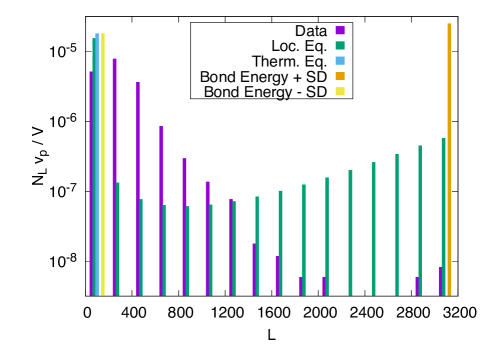
Figure 1: Data on prokaryote cva (labeled ‘Data’, purple bars)compared to equilibria at different values of $\beta\Delta$. Green bars labelled ‘local equilibrium’ show the equilibrium arising from the local temperature derived from the energy $E$ and the particle density $N/V$ giving $\beta\Delta=-2.99$ for this case. Blue bar at left labelled ‘Thermal Equilibrium’ shows the equilibrium associated with ambient external temperature of 293K corresponding to $\beta\Delta=-3.78$. Orange bar labelled ‘Bond energy $+$ SD’ shows the population distribution which would arise at ambient external temperature if the value of $\Delta$ were shifted from its average observed value to that value plus the observed standard deviation of the empirical distribution of bond energies giving $\beta\Delta=-2.28$. (The orange bar is not visible because it is identical to the blue bar.) ‘Bond energy $-$ SD’ (yellow bar) shows the population distribution which would arise at ambient external temperature if the value of $\Delta$ were shifted from its average observed value to that value minus the observed standard deviation of the empirical distribution of bond energies giving $\beta\Delta=-5.28$. Note the dramatic sensitivity of the equilibrium distribution corresponding to ambient temperature arising from varying the bond energy over its range of uncertainty and the similarity of the observed distribution to an equilibrium distribution arising from the much higher ‘local’ temperature (green bars) derived from the energy and the particle density. The values $-2.2$ kcal/mol and $0.875$ kcal/mol for the average and standard deviation respectively of the protein bond energies are from martin1998free . Figure is adapted from intoyhalleypopulations .

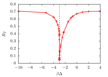
Figure 2: $R_{T}$ as a function of $\beta\Delta$ for the prokaryote prokary- ote Corynebacterium variable DSM 44702 (KEGG code cva From Fig. 5 of reference intoyhalleypopulations . Here $R_{T}$, defined in equation 1, is a measure of disequilibrium, $\beta=1/k_{B}T$ where $T$ is the absolute temperature and $\Delta$ is the binding energy of a monomer-monomer bond (peptide bond in this application). The dashed vertical line is at $\beta\Delta=-\ln 20$, the predicted value of the minimum arising from the hypotheses tested in this paper.

The key point is that the length distribution varies quite smoothly across the range of lengths up to about 2200 monomers , whereas, if we use measured peptide bond energies and room temperature we find equilibrium distributions corresponding to essentially all very long polymers (the yellow bar in the figure), or, with a slight adjustment of the bond energy parameter, all dissociated amino acids (the blue bar). It is hard to see how the length distribution observed could have ever been close to an equilibrium one at room temperature. If the ambient temperature were higher, then the length distribution could be more uniform (as shown,for example, in the green bars in Fig.1) , but in such an environment peptide bonds would be continually breaking and reforming in a dynamical chemical networktaran . Using the proteome population data in another way on the same system we calculated the quantity

$$R_{T}=\sqrt{\sum_{L}(N_{L}-\overline{N_{L}(\beta\Delta)}))^{2}}/(\sqrt{2}V\rho)$$ (1)

as a function of $\beta\Delta$ as a measure of how far from equilibrium the observed polymer length distribution $\{N_{L}\}$ was from equilibrium at a temperature $T=1/k_{B}\beta$ . Here $\rho$ is the volume density of polymers and $V$ is the system volume. With $l_{max}$ defined as the maximum observed polymer length, $R_{T}$ is a Euclidean distance in the $l_{max}$ dimensional space of the $l_{max}$ tuples $\{N_{L}\}$ normalised to lie between 0 and 1. $\overline{N_{L}(\Delta\beta)}$ is the equilibrium distribution when the system is exposed to a thermal bath with an external temperature $1/k_{B}\beta$. $\Delta$ is the binding energy of the covalent bonds connecting the monomers of the model. For peptides it is negative, and we treat mainly that case here.

The result from that paper , shown in Fig. 2 indicates that the distribution observed would be close to equilibrium (as indicated by the small value of $R_{T}$, ) with a thermal bath at a temperature around 400K (using the value -2.2 kcal/mol , taken from reference martin1998free ), for the peptide bond energy, negative because the bond is unstable in aqueous solution. We suggested that this might be an indication that the precursor to the proteome formed at that high temperature, and then became fixed by rapid quenching to a lower temperature closer to current ambient temperature as anticipated in the experiments reported inmatsunoa -matsunoc .

We also noted that the evaluation of a so-called ‘local’ measure $R_{L}$ , defined in detail in the next section (equation (8)), of the distance of the observed length distribution from isolated equilibrium , (see also intoyhalleypopulations ) and also obtained from the proteome data, was close to the minimum value found from the data displayed in Fig. 2. ($R_{L}$ is defined by an equation identical to (1) except that the equilibrium distribution is determined by use of the total energy of the polymer system as well as the total polymer density and the temperature $1/k_{B}\beta$ is not fixed, but is determined by maximization of the entropy, given the energy and the density. Please see intoyhalleypopulations and the next section for more details.) That suggested to us that the precursor had formed in an isolated, nearly equilibrium system at around 400K and the population distribution had then been fixed by quenching. Finally we noted that the value of 400K, given the value of the average peptide bond energy $\Delta$ reported in martin1998free gave a value of $\beta\Delta$ quite close (vertical dashed line in the figure) to $-\ln b$ when $b$, the number of available monomers, takes the value $b=20$, the well-known number of amino acids used in forming the proteins of the biosphere. In the so-called ‘Gibbs limit’ of our equilibrium expressions for equilibrium length distributions, as defined in intoyhalleypopulations and also in the Appendix to this paper, that value of $\beta\Delta$ would give an average value of $\delta\overline{N_{L}}/\delta L$ of zero, thus allowing a wide and rapid exploration of the polymer state space at that temperature. (Here $\delta\overline{N_{L}}$ and $\delta L$ denote finite increments.)So our third suggestion was that quenches from that temperature were more likely to lead to formation of a rare, autocatalytic system with lifelike properties, such as disequilibrium, metastability, high rates of reaction and exponential population growth, after quench because more possibilities were explored in high temperature states at that temperature. Finally we suggested that, at large $b$, the temperature at which the average value of $\delta\overline{N_{L}}/\delta L$ is zero would be such that $\beta\Delta\approx-\ln b$.

In this paper, we report model simulation results which test these ideas by explicitly modeling the conjectured quenches with our Kauffman-like model previously reported in reference conditions . The model is an abstract, or one may say coarse-grained, description of the real proteome system. The only entropic effects which are included are those associated with the combinatorial degeneracies associated with the availability of a more than 1 monomer in polymer formation. That abstraction permits us, in the model, to focus attention on the effects of such degeneracies, which are the root cause of Eigen’s paradox as discussed above. Since these combinatorial, that is informational, aspects of the entropy are associated with the formation and dissociation of covalent bonds which are significantly stronger than the hydrogen bonds and van der waals forces which determine more detailed aspects of biopolymer chemistry, we say that our model is coarse grained in energy, implicitly averaging over such smaller energy effects (which of course are essential for more detailed modeling of life). Our simulation resources limit us to computations up to 7 ($=b$) types of monomers. (Some statements about the large $b$ limit will turn out to be possible by analytical means.) However, as we will discuss in detail in section 4, several aspects of the above conjectures turn out to be consistent with results from the simulated quenches.

In the next section we describe the model of reference conditions and indicate how quenches were simulated and what was measured in the simulation data. The third section states our four conjectures concerning the expected results of the simulations based on the qualitative discussion above. Section 4 summarizes results of the simulations compared with those expectations. Section 5 contains conclusions and a brief discussion of the conditions in ocean trenches and ridges which might result in huge numbers of the envisioned quenches occurring over millions of years and resulting in a substantial probability of fixing a rare, autocatalytic network with lifelike properties.

II Model and Simulation Methods

The model used for quench simulations is fully described in conditions . As in wynveen and elsewherekauffman ,others , artificial chemistries associated with abstracted polymers are generated consisting of strings of digits representing monomers. The polymers undergo scission and ligation. The parameter $p$ controls the probability that, in a given realization, any possible reaction involving polymers up to a maximum length $l_{max}$ is included in the network. (We have regarded the small values of $l_{max}$ imposed by computational limitations to be a flaw, but the recent discoveryleslie of ubiquitous ‘microproteins’ in contemporary organisms may suggest that our simulations of short polymers are more relevant to prebiotic chemistry than previously thought.) Each reaction in the network is randomly assigned one enzyme from the species present in the network. The number of enzymes assigned per reaction here is different from the very large number of enzymes per reaction in the model of reference conditions . The choice here was made to more closely describe the situation in real proteomes. A more complete account of the dependence of the model on the number of enzymes will appear laterqianyi . From the resulting chemical networks we select, as we did previously wynveen , those which are ‘viable’ by which we mean that there is at least one reaction path from a ‘food set’ of small polymers to at least one polymer of maximum length. The probability that a network is viable is then found as the ratio of the number of realizations of the network which are viable divided by the total number of realizations.

As in wynveen but differently from the model described by us in intoy , we assume here that the system is ‘well mixed’ and no effects of spatial diffusion are considered. To any ‘polymer’ ( string) of length $L$ we attribute an energy $-(L-1)\Delta$ where $\Delta$ is a real number which is the bonding energy between two monomers. The total energy $E$ of any population $\{n_{m}\}$ of polymers in which $n_{m}$ is the number of polymers of type $m$ is $E=-\sum_{L=1}^{l_{max}}(L-1)N_{L}\Delta$. Here the $N_{L}=\sum_{m\ of\ length\ L}n_{m}$ is the same set of macrovariables used in wynveen and intoy . The total number of polymers $N$ is $N=\sum_{L=1}^{l_{max}}N_{L}$.

In the simulations described here and motivated by the discussion in the introduction, we take $\Delta$ to be negative. That means, consistent with experiments on peptide bond formation in aqueous media, that the energy of each bond is positive, meaning that it costs energy to make a bond. Here $\beta$ is assumed to be positive so that the relevant parameter $\beta\Delta<0$. The configurational entropy associated with a coarse grained prescription of the state given by the numbers of molecules $N_{L}$ for each length $L$ between $L=1$ and $L=l_{max}$ is found by maximizing the total configurational entropy for any set $\{N_{L}\}$ as given by the general Boltzmann definition $S/k_{B}=\ln W$ (valid whether the system is in equilibrium or not) with respect to the $\{N_{L}\}$ subject to the constraint $\sum_{L=0}^{l_{max}}N_{L}=N$. Here $W$ is the number of sets of polymers possible consistent with the set $\{N_{L}\}$ given that there are $b$ different monomers available at each monomer site in all the polymers. This is a standard problem in statistical physics landau with the result

$$S/k_{B}=\sum_{L}\left[\ln((b^{L}+N_{L}-1)!)-\ln(N_{L}!)-\ln((b^{L}-1)!)\right]$$ (2)

for the general form of the entropy (whether the system is in equilibrium or not. Also see our paper wynveen for more details.) In our simulations the polymers are not in equilibrium but, in addition to the nonequilibrium distributions calculated from kinetics, we also calculate the distributions $\{\overline{N_{L}}\}$ associated with local equilibrium and equilibrium with a temperature bath at temperature $T$ continuously during the simulations. Those distributions are found by maximizing the entropy given above with respect to the variables $\{N_{L}\}$ subject to different constraints depending on whether the equilibrium attained is that resulting from an open system in contact with a thermal bath at fixed temperature $T=1/k_{B}\beta$ or, on the other hand, is sufficiently isolated to permit it to attain local equilibrium consistent with the current value of the total energy $E$. In the former, open, case, the maximization is carried out taking account of the constraint with a Lagrange multiplier $\mu$ which is the chemical potential whereas in the second, closed or local case, the maximization is carried out taking both constraints (energy and particle number) into account with Lagrange multipliers $\mu$ and $\beta=1/k_{B}T$, which are determined from the inputs $N$ and $E$ (as described in detail in reference conditions ). In both cases, $\overline{N_{L}}$ is found to have the form

$$\overline{N_{L}}={{b^{L}-1}\over{\exp(-\beta\mu-\beta\Delta(L-1))-1}}$$ (3)

This expression is formally equivalent to that found for a bose gas in elementary quantum statistical mechanics although this model has no explicitly quantum features and no quantum effects are suggested or implied . See references wynveen and landau . In the ‘Gibbs limit’ in which $b^{L}>>N_{L}>>1$ all these expressions reduce to the familiar classical Boltzmann equilibrium formulae as discussed in landau and the appendix to this paper, for example. That limit applies in the present case for proteins in most biological contexts. But for RNA, for which $b=4$, it is only valid for large $L$ and corrections to the Boltzmann equilibrium formulae are nonnegligible for many of our simulations. To determine the isolated equilibrium state we compute $\beta$ and $\mu$ from the known energy $E$ and polymer number $N$ by solution (on the fly during the simulations) of the equations

$$E=-\sum_{L=1}^{l_{max}}(L-1)\overline{N_{L}}\Delta$$ (4)

and

$$N=\sum_{L=1}^{l_{max}}\overline{N_{L}}$$ (5)

whereas to determine the equilibrium state resulting from equilibrium with a temperature bath we fix $\beta$ and determine $\mu$ by solution, again on the fly, using the equation 5 . Note that, in this formulation and throughout the paper, references to ‘equilibrium’ refer to maximization of the configurational entropy, constrained only by the number of polymers and the external temperature (when it is specified) or the total energy. Thus we mean maximization given that all the polymer configurations in the model are ‘accessible’, whereas in some work in chemical statistical mechanics, further constraints are applied, arising from the assumption that some states are kinetically ‘inaccessible’. Such kinetic inaccessibility does occur in our models, through the kinetic model described next, but it does not enter our definition of the equilibrium states.

During the dynamics simulation, the temperature enters the dynamics through the factors $k_{d}$ in the following kinetic Master equation (equation (6)).

$$dn_{l}/dt= \sum_{l^{\prime},m,e}[v_{l,l^{\prime},m,e}(-k_{d}n_{l}n_{l^{\prime}}n_{e}+k_{d}^{-1}n_{m}n_{e})$$ (6)

$$+v_{m,l^{\prime},l,e}(+k_{d}n_{m}n_{l^{\prime}}n_{e}-k_{d}^{-1}n_{l}n_{e})].$$

Here $n_{l}$ is the number of polymers of species $l$, $v_{l,l^{\prime},m,e}$ is proportional to the rate of the reaction $l+l^{\prime}{{e}\atop{\rightarrow}}m$,$e$ denotes the catalyst, $l$ and $l^{\prime}$ denote the polymer species combined during ligation or produced during cleavage, and $m$ denotes the product of ligation or the reactant during cleavage. This model for the dynamics, defined by the Master equation, is stochastically simulated using the Gillespie algorithmgillespie . A parameter $p$ (in $[0,1]$) controls the sparsity of reactions in the network. With probability $p$, each reaction rate has a finite value $v_{l,l^{\prime},m,e}$ or $v_{m,l^{\prime},l,e}$ but the rate is zero with probability $(1-p)$ for each possible reaction. The values of $v_{l,l^{\prime},m,e}$ or $v_{m,l^{\prime},l,e}$ are fixed (from a uniform distribution in $[0,1]$) during the dynamical simulations but the values of the parameters $k_{d}$ are not. The latter are fixed by the detailed balance condition

$$k_{d}^{2}=\overline{n_{m}}/(\overline{n_{l}}\ \overline{n_{l^{\prime}}})$$ (7)

where, in the simulations reported here, the equilibrium distributions $\{n_{l}\}$ in the last expression are always taken to be those associated with equilibrium with an external thermal bath with a fixed parameter $\beta$. We started all the simulations reported in this paper with a ‘food set’ of 500 randomly selected (from the $b(b+1)$ available) monomers and dimers. Some results do depend on the choice of the starting food set. However we are assuming, as in much work on the origin of life, that the problem is to understand how lifelike systems emerge from collections of small, interacting molecules, so that starting from monomers and dimers will give relevant insights. During the simulations, the simulated systems are ‘fed’ by maintaining the population of dimers and monomers above a specified minimum usually taken to be 500 . (Thus the system is ‘open’blokhuis .) The system is continually driven toward equilibrium with the external thermal bath but many simulated systems do not achieve either local equilibrium or equilibrium with the external bath because of the kinetic blocking imposed by $p<1$ and because of the ‘feeding’. As in our previous work, including that described in conditions and wynveen , we assume that lifelike chemical systems will be metastable states far from equilibrium and select and count such states to obtain a quantitative indication of how likely our models are to result in lifelike states.

As in intoyhalleypopulations and conditions we compute two Euclidean distances $R_{L}$ and $R_{T}$ in the $l_{max}$ dimensional space of sets $\{N_{L}\}$ which characterize how far the system of interest is from the two kinds of equilibria described above:

$$R_{L}=\sqrt{\sum_{L}(N_{L}-\overline{N_{L}(\beta(E,N),\mu(E,N))})^{2}}/(\sqrt{2}N)$$ (8)

for distance from the locally equilibrated state and

$$R_{T}=\sqrt{\sum_{L}(N_{L}-\overline{N_{L}(\beta,\mu(\beta,N)}))^{2}}/(\sqrt{2}N)$$ (9)

for distance from the thermally equilibrated state. The normalization factors in these equations differ from that in equation 1 because, in equation 1 we took account of polymer dilution and used experimental data on polymer volume density instead of total polymer number $N$. The normalizations are chosen in each case so that the resulting quantities $R_{T}$ and $R_{L}$ lie in the interval $[0,1]$ permitting the model values to be compared with the experimental ones. Alternative measures of the degree of disequilibrium in the context of study of polypeptide systems have been proposedstopnitzky and we have used alternative formulations in references wynveen and intoy . The formulation used in this paper and in intoyhalleypopulations and conditions has the advantage of discriminating between local equilibrium, which would be achieved by the system in isolation and the global or thermal equilibrium with an external thermal environment, which would be eventually achieved if the system were in contact with an external, equilibrated ‘bath’. The latter distinction has provided valuable insights into the nature of the nonequilibrium states found in our quench simulations. A similar Euclidean measure of disequilibrium in the context of prebiotic evolution was also suggested in reference baum . More details of the simulation methods are described in conditions .

The physical significance of $R_{L}$ and $R_{T}$ is that $R_{L}$ measures the distance in the population space of the current simulation point from the point where it would be if the system had self equilibrated consistent with its total internal energy $E$ but not with any external temperature bath, whereas $R_{T}$ measures the distance in the population space of the current simulation point from the point where it would be if the system had equilibrated to an external temperature bath at temperature $T=1/k_{B}\beta$. One generally expects self equilibration to occur faster than equilibration to an external temperature bath. The temperatures of the corresponding equilibria are often different in condensed matter systems, for example electron temperatures, both in plasmas gonzalez and in solids (eg perrez ) can be different from ion or lattice temperatures respectively and the internal temperature associated with the distribution of nuclear spin directions in NMR experimentsabragam can be different from the lattice temperature (and negative in the latter case.)

In the results cited in section IV the code implementing this model was modified to permit an abrupt change in the parameter $\beta\Delta$ during the simulation of systems in contact with an external thermal bath. In the report of results which follows, we change the value of $\beta\Delta$ from a small negative value to a large one. The values are negative because the free energy of bond formation of peptide bonds in water is negative martin1998free as noted above and the choice of small to large negative values will correspond, in the case that $\Delta$ does not change, to a quench from high to low temperature. We thus refer in the discussion to quenches from high to low temperature, but note that the relevant parameter in the model is the product $\beta\Delta$ (the two factors always occur together) and a similar change in that parameter might be induced by altering $\Delta$ for example by a rapid change in pH pHdependence

III Hypotheses

If the model described in the preceding section adequately describes the coarse grained features of the relevant prebiotic chemistry, then the conjectures concerning the origin of prebiotic chemistry in quenches of interacting amino acids from high to low temperature described in the introduction imply that we should expect the following simulation results within the model:

1. Running at initial high temperature $\beta\Delta_{i}$ and then quenching to $\beta\Delta_{f}$, one should find a minimum, during the low temperature part of the run,in

$$R_{T}(\beta\Delta)=\sqrt{\sum_{L}(N_{L}(\beta\Delta_{f})-\overline{N}_{L}(\beta\Delta))^{2}}/\sqrt{2N}$$ (10)

as a function of $\beta\Delta$ at $\beta\Delta=\beta\Delta_{i}$. Here $N_{L}(\beta\Delta_{f})$ is the value of $N_{L}$ found from the kinetic simulation with external temperature $\beta\Delta_{f}$ and $\overline{N}_{L}(\beta\Delta))$ is the equilibrium expression for $N_{L}(\beta\Delta)$ at the temperature $\beta\Delta$. We do consistently find such a minimum, though the minimum value of $R_{T}$ varies as discussed later. We denote the value of $\beta\Delta$ at the minimum by $\beta\Delta_{min}$ . Then the hypothesis states that $\beta\Delta_{min}=\beta\Delta_{i}$. We will present numerical evidence that, within the model, this is approximately true when $p$ is sufficiently large.

The significance of this is that if an experimental system, such as one of the proteomes we studied previously, exhibits such a minimum in $R_{T}(\beta\Delta)$ with $N_{L}(\beta\Delta_{f})$ replaced by the experimental values of $N_{L}$ then the $\beta\Delta$ at which a minimum in $R_{T}(\beta\Delta)$ occurs is a signature of the temperature at which the system formed before quench. Thus, since the proteomes had such a minimum at around 400K, our simulations would support the idea that the system formed from a quench at a high temperature around 400K. (See Fig. 2.)

2. The high temperature at which equilibrium should occur most easily should be the one which gives

$$(1/l_{max})\sum_{L}\delta\overline{N_{L}}/\delta L(\beta\Delta)=0.$$ (11)

(Here $\delta\overline{N_{L}}$ and $\delta L$ denote finite increments. In implementation we take $\delta L=1$.) We call the solution to this equation $\beta\Delta_{flat}$.

To explain the motivation for this hypothesis further, we refer to the discussion of Fig. 1 in the introduction to this paper. There we pointed out that very small changes in the assumed binding energy of peptide bonds produced very large changes in the equilibrium polymer length distribution if the temperature were near ambient. So at those, low, temperatures the equilibrium distribution would be very likely to be either almost all monomers or almost all polymers of maximum length (the blue and orange bars in the Fig.). If the lengths were distributed in that fashion in prebiotic conditions then the kinds of interactions possible would be highly constrained if the system were near equilibrium. That, in turn would greatly slow the rate at which polymer configurations were naturally explored by the kinetics, slowing, in turn, the natural search (in a dynamic network as envisioned in taran ) for the rare combinations which turn out to be lifelike. However the actual distribution of protein lengths in prokaryotes is usually like that shown for one of them by the purple bars in Fig. 1 and such a distribution can be envisioned to permit the kind of natural search required. Therefore we sought, in formulating hypothesis 2, a condition on the initial temperature which would require that the equilibrium length distribution be reasonably flat so that, if the system were near equilibrium in the high temperature phase before quench, it would be capable of the kind of natural search envisioned in taran and by us. Equation (11) realises that aim by requiring that the average discrete derivative of $\overline{N_{L}}$ with respect to $L$ be zero. However if the temperature is high and gives a relatively flat distribution as required by equation (11), then, in the high temperature phase of the simulation before quench the system will most easily come close to equilibrium. That would say that if, at high temperatures, one computes $R_{T}(\beta\Delta_{i})$ in our model (with BOTH $\beta\Delta$ arguments in the definition =$\beta\Delta_{i}$) then one should find the smallest $R_{T}$ at the value of $\beta\Delta_{i}$ for which 11 is true, as postulated in Hypothesis 2.

3. The most lifelike states after quench should occur when the initial high temperature state coincides with the minimum described in 2. To characterize this prediction quantitatively requires a more detailed statement of the definition of ‘lifelike states’ as we will discuss in the next section.

4. The solution to $(1/l_{max})\sum_{L}\delta\overline{N_{L}}/\delta L(\beta\Delta)=0$ will be at $\ln b=-\beta\Delta$ in the large b limit and that is the appropriate limit for the proteome systems.

IV Results

Before describing results of tests of the hypotheses of section III we show an example of how $R_{T}$ characteristically behaves in Gillespie simulation time during a subset of our simulated quenches. In Fig. 3) the black circles show average values of $R_{T}$ over 30 runs on the same network in a simulation at a high temperature ($\beta\Delta=-.1$), well above ambient temperature. The high temperature systems start far from the equilibrium associated with the external temperature ,because all simulations start with just a randomly selected food set, but quite rapidly approach a state near equilibrium. Here, as in most cases and even without significant kinetic blocking, our simulations do not go all the way to equilibrium because they are continually being ‘fed’ by maintenance of the food set population. The red triangles show what happens when the simulations are repeated starting with the same high temperature with a quench at time zero to a lower temperature ($\beta\Delta=-4.$). The systems attain a high value of $R_{T}$ after quench because the equilibrium point has moved in the species space, but the instantaneous populations have not. The systems then move closer to equilibrium at the lower temperature but do not achieve it. To see if the quench has produced systems farther from equilibrium than a simulation entirely at the lower temperature would do, we also show ,in the green symbols, the results of a simulation on the same systems when the external temperature remains at the low value ($\beta\Delta=-4.$) throughout . The green curve flattens at a higher value of $R_{T}$ than the high temperature one (black symbols) but below the quenched values (red symbols) indicating that the quench has produced systems farther from low temperature equilibrium than would simulating from the lower temperature from the start. However the effect is relatively small in these examples. A more comprehensive set of data evaluating the effect of quenching on disequilibrium appears in Fig. 9.

In Fig. 4 we show the total polymer populations as a function of the number of reaction steps for the same ensemble of realizations of the model. The quench has a much bigger effect on this variable: The final number of polymers is much larger throughout times after the quench than it is at low temperature after a quench and also bigger than the final number from the run at the higher temperature throughout. Of equal interest, the quenched systems continue to grow rapidly after quench whereas both the low and high temperature runs show very little population growth near the end of the runs. Part of the growth in the total number of polymers after quench is due to the increased rate of scission relative to ligation at the lower bath temperature.

In these examples we thus have preliminary evidence that three properties deemed lifelike, namely disequilibrium (measured by $R_{T}$), population size and population growth rate, are enhanced by quenching from high temperatures. Note that, in the model, the temperature always occurs in the combination $\beta\Delta$ so that identical results could also be achieved by a sudden change in $\Delta$ as, for example, might be achieved by a sudden change in pH.

The ‘error bars’ in the figures indicate standard deviations in the distribution of results over this ensemble and suggest, consistent with our detailed results, that some realizations can experience much higher values of disequilibrium and growth rate after quench.

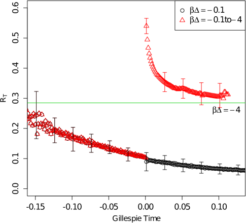
Figure 3: Average over 30 runs on different networks of the value of $R_{T}$ versus Gillespie simulation time. Gillespie times have been shifted by a constant so that the quench always occurs at Gillespie time =0. Some data from times earlier than Gillespie time (as shifted) less than -0.15 which arise from noisy initial transients have been omitted. Error bars indicate standard deviations over the ensemble. Total simulation time was fixed to be $3\times 10^{6}$ reaction steps and quench was applied at $3\times 10^{5}$ reaction step. Parameters are $p=0.1280$, $b=4$, $l_{max}$=7.

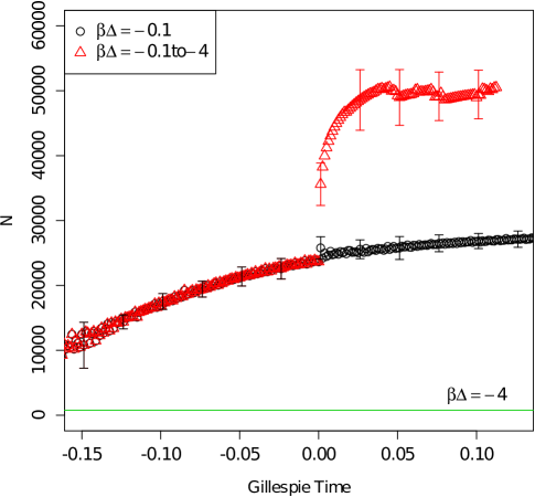
Figure 4: Average over 30 runs on different networks of the value of N, the total number of polymers, versus Gillespie simulation time. Error bars indicate standard deviations over the ensemble. Parameters are $p=0.1280$, $b=4$, $l_{max}$=7.

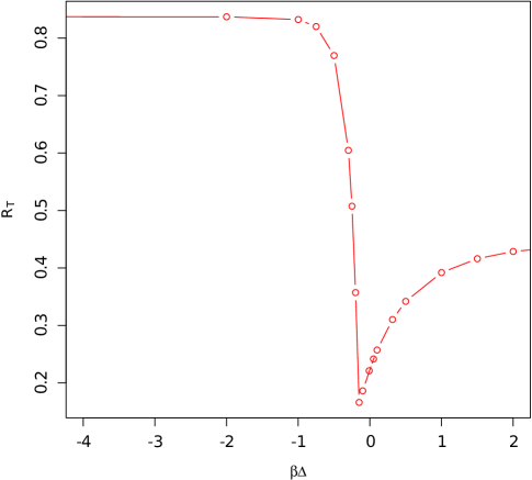
Figure 5: $R_{T}$ from equation 10 calculated from a dynamic simulation with $b=4$, $l_{max}=7$, $p=0.1280$, $\beta\Delta_{i}=-0.1$ and $\beta\Delta_{f}=-4$. Compare 2 which was obtained from proteome data.

In the following data we show results bearing on the validity of the hypotheses we consistently fixed the parameters $\beta\Delta_{f}=-4.,l_{max}=7$ and , where not specified otherwise, $b=4$. The value of $\beta\Delta_{f}$ was chosen to approximately match the value for peptide bonds under ambient conditions. The values $b=4$ and $l_{max}$ are approaching the limit imposed by constraints on available simulation resources. Networks had reactions with 1 enzyme per reaction. Results are presented for a series of $p$ values in the model, since the $p$ value turns out to be significant.

Regarding hypothesis 1. We show values of $\beta\Delta_{min}$ as a function of $\beta\Delta_{i}$ for a series of $p$ values in Fig. 6. The data get closer to the hypothesis as $p$ increases and $\beta\Delta_{i}$ becomes less negative corresponding to higher temperatures and a more connected chemical network.

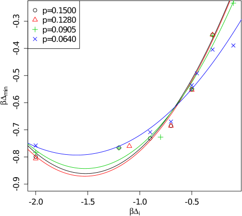
Figure 6: Simulated values of $\beta\Delta_{min}$ versus $\beta\Delta_{i}$ for various $p$ values. The final temperature are set so that $\beta\Delta_{f}=-4$. Each data point comes from an average over 40 500 realizations. The simulation used values $b=4$, $l_{max}=7$. The smooth curves show the result of fitting these data, for each value of $p$ to a quadratic function of $\beta\Delta_{i}$ as explained in the text.

To explore hypothesis 1 further we fit the function $\Delta\beta_{min}=f(\Delta\beta_{i})=f(0)+f^{\prime}(0)\Delta\beta_{i}+(1/2)f^{\prime\prime}(0)(\Delta\beta_{i})^{2}$, ie the first terms in a Taylor series in $\Delta\beta_{i}$ to the data in Fig. 6 for five $p$-values between .05 and .3 with results indicated by the smooth curves in the Fig.. Hypothesis 1 states that we will find $f(0)=0,f^{\prime}(0)=1,f^{\prime\prime}(0)=0$ . Results are shown in Table 1. The hypothesis is quite nearly confirmed for the larger values of $p$.

Table 1: Polynomial fit parameters for the data in Fig. 6

p	$f(0)$	$f^{\prime}(0)$	$f^{\prime\prime}(0)/2$
0.1500	-0.09019 +- 0.04496	1.01408 +- 0.10566	0.33341 +- 0.04801
0.1280	-0.09674 +- 0.04552	1.01314 +- 0.11502	0.33139 +- 0.05181
0.0905	-0.13961 +- 0.04393	0.92138 +- 0.10938	0.30185 +- 0.04991
0.0640	-0.27957 +- 0.04638	0.63970 +- 0.11963	0.19924 +- 0.05271
0.0226	-0.63764 +- 0.01819	0.12222 +- 0.04276	0.03128 +- 0.01943

To explore the dependence of this result on $b$ we carried out a similar analysis for $b=2,3,$ and $5$ and show the results for the fitting parameters as a function of $p$ for five $p$-values between .05 and .30 with results shown in Fig. 7 . As $b$ gets larger the quadratic term gets smaller, indicating that the hypothesis works for larger and larger values $\beta\Delta_{i}$ and consistent with the suggestion that at the biologically relevant value of $b=20$ it will continue to be valid up to values of $\beta\Delta_{i}=-\ln 20$.

Note that when $b$ gets larger, even a relatively small $p$ gives a slope near 1. We conclude that for large $b$ systems such as the one in the proteomes with $b=20$ it’s very likely that $\beta\Delta_{i}=\beta\Delta_{min}$ in agreement with hypothesis 1. Thus our previous inference that the value for $\beta\Delta_{min}$ taken from the proteome data was an indicator of the temperature from which the proteome had been quenched on the early earth is consistent with our model.

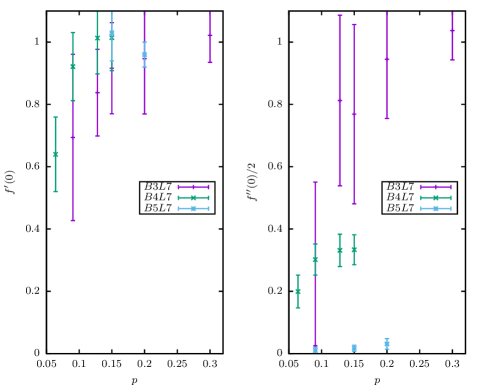
Figure 7: Values of the slope (left) and curvature (right) of fits to the data in Fig. 6 and similar data for $b=2,4$ and $5$ to quadratic functions of $\beta\Delta_{i}$ as a function of $p$ as explained in the text. Error bars indicate standard errors.

To test hypothesis 2 we calculated solutions to equation 11 numerically for values of b=2,3,4,5,6,7. Hypothesis 2. states that the value of $\beta\Delta_{i}$ at which

$$R_{T}(\beta\Delta_{i})=\sqrt{\sum_{L}(N_{L}(\beta\Delta_{i})-\overline{N}_{L}(\beta\Delta_{i}))^{2}}/\sqrt{2N}$$ (12)

is minimum (termed $\beta\Delta_{min}$) should be at the same value of $\beta\Delta_{i}$, termed $\beta\Delta_{flat}$ at which (11) is true. (Note that, in equation 12, BOTH arguments $\beta\Delta$ are at $\beta\Delta_{i}$ (the ’hot’ value) unlike equation 10. Hypothesis 2 is a statement only about the ‘hot’ phase.) There is a complication here because $\overline{N}_{L}(\beta\Delta_{i})$ depends on $\mu\beta$ which, in turn, depends on the total number $N$ of polymers present in the current state of the system. To determine $\beta\Delta_{min}$ we used that current value of $N$ at each value of $\beta\Delta_{i}$ in equation (12) and then used the $N$ value at $\beta\Delta_{min}$ to give a value for $\beta\mu$ to use in solution of equation (11) for $\beta\Delta_{flat}$. The values of $\beta\Delta_{min}$ and $\Delta\beta_{flat}$ are compared for $b$=2,3,4,5,6,7 and $p=0.0226,l_{max}=7$ in Fig. 8. The trends in the two quantities are the same and the values are close to one another but not identical. As $b$ gets larger they get closer. We conclude that hypothesis 2 is likely to be a very good approximation when $b$ is large, as in the proteomes.

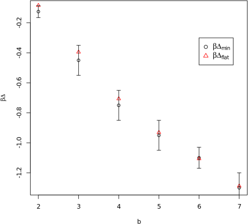
Figure 8: $\beta\Delta_{flat}$ and $\beta\Delta_{min}$ versus $b$. $\beta\Delta_{min}$ is determined by running simulations with a series of temperature $\beta\Delta_{i}$ and finding minimum $R_{T}(\beta\Delta_{i})$. The error bars are determined when a $\beta\Delta_{i}$ gives a $R_{T}(\beta\Delta_{i})$ that is within $10\%$ difference of $R_{T}(\beta\Delta_{min})$. .

Regarding hypothesis 3, we first tested for the enhancement of $R_{T}$, termed $\Delta R_{T}$ in the cold phase, relative to the value obtained in the same network with the same starting conditions when the temperature was low throughout the run. The hypothesis states that $\Delta R_{T}$ should be largest when $\beta\Delta_{i}-\beta\Delta_{flat}$ is zero. We show results for three $p$ values in Fig. 9. In all cases, the enhancement rises sharply as $\beta\Delta_{i}\rightarrow\beta\Delta_{flat}$ confirming hypothesis 3 for the lifelike property of disequilbrium. Qualitatively, the enhancement occurs because at the high temperature, the systems get close to the internal equilibrium population distribution imposed by their total energy and retain a distribution of polymer lengths close to that value after quench. The enhancement increases with $p$, possibly because the high temperature phase equilibrates more effectively before quench as $p$ increases. However for very large $p$ the effect of the stabilization of nonequilbrium states by quenching is expected to become less effective because the denser network will allow equilibration even in the low temperature state.

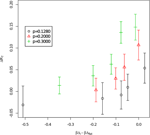
Figure 9: Enhancement of $R_{T}$ as a function of $\beta\Delta_{i}-\beta\Delta_{flat}$ for various values of $p$. $\beta\Delta_{f}=-4$,$l_{max}=7$, $b=4$. Each point is from between 20 and 50 simulations with smaller numbers of simulations for larger values of $p$. Error bars indicate standard deviations.

To study the effects of quenching on other, possibly lifelike , properties we applied a series of filters to the ensembles of systems obtained by quenching and show results in Fig. 10. (Quenching from the high to low environmental temperature does not enhance $R_{T}$ significantly for the range of $p$ values used here, but does enhance $R_{T}$ at larger $p$ values as indicated in Fig. 9.)

In part c. of Fig. 10 we show results of imposing an additional filter which excludes results in which the reaction rate per polymer in the final steady state is below a fixed value. This ‘dynamics filter’ is different than the one imposed on our results in references conditions ; wynveen ; intoy . To make the cut we require that the total number of reactions per polymer in the final steady state divided by the gillespie time elapsed during that steady state part of the run be larger than a fixed value which, in the data displayed in Fig. 10, we chose to be 10 reactions per unit of Gillespie time. (Roughly, one unit of Gillespie time corresponds to the average rate of ligation and scission.) There is a very large enhancement of reaction rate due to quenching.

Finally, in part d of Fig. 10 we show the effects of further filtering to isolate the final steady states showing enhanced to polymer population growth rates. In that cut, we eliminated systems in which the logarithmic derivative of the total number of polymers with respect to Gillespie time was less than 1.

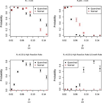
Figure 10: (a) Probability of finding $R_{T}>0.35$ with (Quenched) and without (Normal) quenching, (b) same with $R_{L}$ and $R_{T}>0.35$, (c) Probability of finding $R_{T}>0.35$ and a high reaction rate , (d) Probability of $R_{T}>0.35$, a high reaction rate and a high growth rate. The threshold for the reaction rate cut off is 10 reactions per unit of Gillespie time per polymer. The growth rate cut off eliminates those systems for which $d\ln N/dt<1$ in units of inverse Gillespie time. For the quenched simulations, $\beta\Delta_{i}=\beta\Delta_{flat}$ and $\beta\Delta_{f}=-4$. For the unquenched simulations $\beta\Delta_{i}=\beta\Delta_{f}=-4$. $b=4$, $l_{max}=7$, for both cases. From data on 50 to 700 realizations with more simulations for the smaller values of $p$. Error bars show standard deviation from the average over the simulations for each parameter set.

We made a study of the dependence of the observed $R_{T}$ quench enhancement on the initial and final temperature parameters $\beta\Delta_{i}$ and $\beta\Delta_{f}$ for the case $b=4$ with results shown in Fig. 11. High initial temperatures ($|\beta\Delta_{i}|$ small) and relatively high final temperatures ($|\beta\Delta_{f}|$ also small but larger than $|\beta\Delta_{i}|$) are favored. In the case that $|\beta\Delta_{i}|$ is small though larger than $|\beta\Delta_{f}|$, there is a wide range of $|\beta\Delta_{f}|$ which is predicted to give substantial $R_{T}$ enhancement in the quench However, in the envisioned application, final values of $\beta\Delta_{f}$ are expected to be as large as -4 and in that case, the range of $|\beta\Delta_{i}|$ which gives a large enhancement is predicted to be quite narrow. Such estimates can be useful to experimentalists exploring the parameter space to determine the conditions under which lifelike systems are most likely to be produced by quenching.

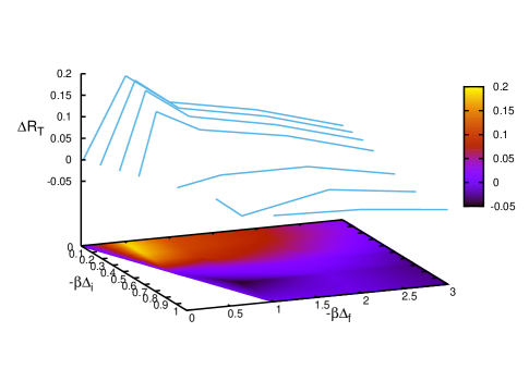
Figure 11: Enhancement in $R_{T}$ arising as a consequence of a qeunch as a function of the initial and final values $\beta\Delta_{i}$ and $\beta\Delta_{f}$ of the parameter $\beta\Delta$. For all these quenches $p=0.0761$, $b=4$, $l_{max}=7$ and the quench was applied at reaction step =$10^{5}$. Each data point is an average over 400 simulations (80 networks and 5 realizations per network)

We explored the distribution of $R_{L}-R_{T}$ values in the final simulation states in systems running at low temperatures with the corresponding distributions when the final state is at the same final temperature but has been quenched from a high temperature. Results are shown in Fig. 12 for $b=4$, $l_{max}=7$ and $p=0.0950$ $\beta\Delta_{i}=-0.01$ $\beta\Delta_{f}=-4.$ Remarkably, more states with longer average polymer lengths appear in the high $R_{T}$ part of $R_{L}-R_{T}$ plane. These states are quite close to the region of the $R_{L}-R_{T}$ plane where the values for real proteomes are found intoyhalleypopulations as indicated by the box in the Fig. and the results indicate that the quench has stabilize the bonded, long polymers.

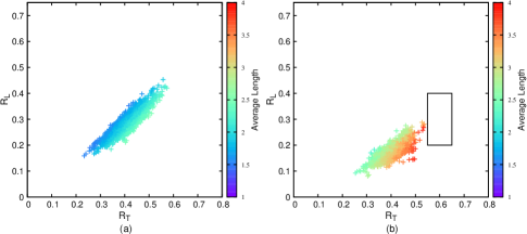
Figure 12: At right: Values of $R_{L}$, $R_{T}$ found in 1,200 simulations of the model with $b=4$, $l_{max}=7$ and $p=0.0905$, $\beta\Delta_{i}=-0.01$, $\beta\Delta_{f}=-4$. At left: Results with the same parameters and networks but with $\beta\Delta=-4$ throughout the runs (no quench) as a control. The box indicates the region in which real proteomes were found in reference intoyhalleypopulations . The color scale indicates the average polymer length in the final, quenched state.

Hypothesis 4 is a statement about equilibrium. The values of $\beta\Delta$ at which $(1/l_{max})\delta\overline{N_{L}}/\delta L=0$ are evaluated numerically from $b=2$ to $b=20$ various values of $N/b^{l_{max}}$ in Fig. 13 . They converge to the $\ln b=-\beta\Delta$ when $N/b^{l_{max}}<<1$ as shown analytically in the Appendix. For proteins in a proteome, $N$ is of the order of $10^{6}$ and $b^{l_{max}}\approx 20^{2000}=4\times 10^{2000}$ so the limit is easily realized.

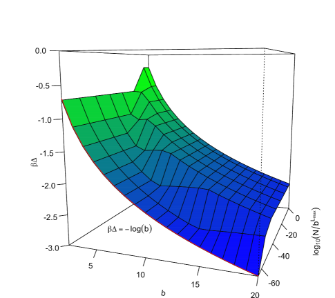
Figure 13: $\beta\Delta_{flat}$ as a function of $b$ and $N/b^{l_{max}}$. The red line is the relation $\beta\Delta_{flat}=-\ln b$.

V Discussion and Conclusions

In summary, the simulations reported here on a previously developed model are consistent with the idea posed in our earlier paper, namely that the polymer length distributions observed in existing proteomes might suggest that early life was associated with a higher temperature environment and that the lifelike systems generated in that environment could have been stabilized by a rapid quench to lower temperatures. In doing those simulations we introduced new features in the simulations (but not in the model): Quenches from high to low temperature were incorporated and the dependence of the resulting low temperature steady states on the initial temperature, the final temperature, the number of available monomers $b$ and the maximum polymer length was explored. Of particular note is the strong dependence of the results on the initial, high temperature which needs to be quite precisely tuned to minimize $R_{T}$ to achieve maximum enhancement of lifelike states in the final , low temperature environment. We understand this qualitatively as arising because the low $R_{T}$ in the high temperature state permits rapid bond breaking and formation allowing a full exploration of the state space by the dynamics. The sharpness of the region associated with the minimum in $R_{T}$ arises from the abrupt transition, in the corresponding equilibrium state, from an equilibrium state of nearly all monomers to a state of nearly all maximum length polymers as a function of temperature. That was illustrated for proteome data from the biosphere in Fig. 2 and is also manifested in our simulations. An example from the simulations was shown in Fig. 5 ( This is closely associated mathematically with the Bose-Einstein transition in low temperature physics. However we are working with a finite system, meaning that there are no true phase transitions, we are ultimately concerned with nonequilibrium states and the physics is entirely different and not directly associated with any quantum effects.) Though we are only able to explore it up to $b=7$ we are able to plausibly extrapolate to the protein relevant value of $b=20$ to confirm that the model is approximately consistent with our earlier conjecture intoyhalleypopulations that, from the observed length distributions in the proteome data, we could infer that the prebiotic formation of the first proteomes formed at a temperature of about $-\Delta/(k_{B}\ln b)$ The previously proposed relation for the optimum initial high temperature (minimizing $R_{T}$) of $\ln b=-\beta\Delta$ is approximately consistent with the numerical data extrapolated to large $b$.

Though we have applied our analysis using the ideas described here to proteome data, the same considerations and model might also apply in principle to synthesis of RNA in an RNA-world scenario for the origin of life. The phosphate bonds in RNA are similarly of higher energy in water than the separated nucleotides (so in our formulation $\Delta<0$ as for proteins ). Biology only uses four nucleotides in RNA so we would set $b=4$. The maximum length of RNA in biological systems is much longer than it is for proteins so the expansion parameter $N/b^{l_{max}}$ used in the expansion in the Appendix is likely to be small. However experimental production of collections of nucleotides without any proteins has proved problematic in attempts to experimentally produce models for RNA world scenarios and in contemporary biology RNA generally does not seem to occur without accompanying proteins though RNA replicases have been found which could in principle catalyse biochemical reactions without proteins in an RNA world. On the other hand, relatively isolated systems of proteins such as amyloids and prions exist. These features made it difficult to find data relevant to the RNA world hypothesis with which to compare the results of our model and, for those and other reasons, we have not yet fully explored the possibility of the applicability of our results for the $b=4$ case to nucleic acids in prebiotic chemistry. Note that all of the high temperatures associated with optimal conditions for bond formation in the hypotheses of section III will not coincide as closely in our model when $b=4$ as they do when $b=20$. That would suggest that the high temperature most favorable to quenching of solutions of amino acids to form polypeptides may be more precisely defined than it would be for formation of RNA from nucleotides. Thus, at the optimal high temperature, our quenching mechanism might work better for proteins than for RNA.

We believe that these results may have implications for possible scenarios for the origin of life and also for possible laboratory experiments exploring conditions which could lead to lifelike chemistry in nonbiological contexts. With regard to the former we note that in ocean trenchestrenches liquid water at temperatures well above the boiling point under ambient conditions is continuously being emitted and spilled quite rapidly into cooler water. Such encounters of very hot alkaline water emerging from an ocean trench, for example in a ‘black smoker’, with acidic ocean water at temperatures near 0^o C have been suggestedbarge as possible prebiotic sites where electrochemical processes could lead to the generation of energy carrying small molecules , particularly FeS, that could provide energy for peptide bond formation. In such an environment, we envision that formation of polypeptide networks behaving as in our models might occur and grow. If such processes continued from a very early stage in the earth’s history then a very high rate of continuous quenches could proceed over many hundreds of millions of years. That a few of those very numerous quenches could have resulted in trapping of nonequilibrium dynamic systems out of equilibrium leading in one case to life initiation seems to us at least as plausible as many alternative scenarios which have been proposed.

An advantage of the scenario discussed here is that bonds can be broken and reformed at a high rate in the high temperature phase, thus allowing a wide exploration of the state space, and then be rendered more stable by quenching. Most of those low temperature states will not be lifelike, but if this event occurs many millions of times, some of them may be. The function of the quench in the envisioned scenario is that it could trap those states out of equilibrium with the lower temperature ambient environment associated with the quenched state, thus possibly permitting a promising lifelike configuration which would be rapidly transformed in the high temperature state to evolve and grow in the lower temperature quenched environment. Our simulations are probably underestimating the magnitude of such a trapping effect, because they do not take explicit account of the possibility that the quench could stabilize lifelike states because of the existence of free energy barriers to the hydrolysis reaction leading to scission of peptide bonds. Such barriers are known to lead to survival of some peptide bonds for as long as centuries in the absence of enzymesscissionbarrier , though a lower limit of more like 35 days is likely. Building a model to take explicit account of the existence of such barriers is a high priority for future work and is underway. In preliminary work in this direction, we are making the distribution of reaction rates $v$ temperature dependent to take account of activation free energies.

A similar quenching phenomenon might occur in tidal pools, where the daily cycles of drying and wetting are accompanied by cooling and heating. The temperature differences are not expected to be as large, but an advantage is that the process may be repeated many times on the same system. Bond breaking is also sensitive to pH of the aqueous environment pHdependence and a similar cycling of pH might lead to similar effects in both the ocean trench and tidal pool contexts. All these possibilities require further theoretical and experimental study.

With regard to laboratory experiments, the experiments of Yin et al yin in which solutions of amino acids are dried at high temperature and then redissolved in water for analysis approximate some of the conditions envisioned here for prebiotic evolution. Matsuno et al matsunoa -matsunoc did laboratory experiments in which solutions of amino acid monomers were quenched to low temperature and pressure and length enhancements in the polypeptides produced were observed. Our preliminary analysis of the experiments described in yin and matsunoa -matsunoc gives low values of $R_{L}$ and much larger values of $R_{T}$ nearer 1, in qualitative agreement with our simulation results. However the effects in the experiments are larger than in the simulations: The experimental $R_{L}$ values are smaller and the experimental values of $R_{T}$ are nearer 1 than they are in the simulations. There are several possible reasons for the discrepancy including the primitive character of the model, effects of unrealistically small $b$ or the lack of barriers to dissolution of the bonds in the model. Because the experiments of yin and matsunoa -matsunoc share a similar quantitative discrepancy with the simulations, it is unlikely that the failure to model the details of the drying part of the experiment of yin is the source of the discrepancy. A more detailed analysis of these experiments using the measures employed in this paper will appear later.

VI Acknowledgements

Work was supported by NASA grant NNX14AQ05G, by the Minnesota Supercomputing Institute and by the Open Science Grid.

VII Appendix: Low density expansion of the equilibrium model

Following methods closely related to standard derivationshalleySM of the virial expansion for gases of interacting atoms, we obtain an expansion for $N/b^{l_{max}}$ in the fugacity $z=e^{\mu\beta}$ for the total number of particles in equilibrium as follows: Rewrite equation (5 ) as

$$N/b^{l_{max}}=\sum_{L=1}^{l_{max}}{{{(b^{L-l_{max}}-b^{-l_{max}}})z}\over{(e^{\epsilon_{l}\beta}-z)}}$$ (13)

where $\epsilon_{L}=-\Delta(L-1)$. Expand for small $z$ :

$$N/b^{l_{max}}=\sum_{L=1}^{l_{max}}\sum_{n=0}^{\infty}z^{n+1}e^{-(n+1)\epsilon_{L}\beta}(-1)^{n}(b^{L}-1)b^{-l_{max}}$$ (14)

or reversing the orders of summation

$$N/b^{l_{max}}=\sum_{n=0^{\infty}}z^{n+1}F_{n}(\beta\Delta)$$ (15)

The sums on $L$ in $F_{n}$ are geometric giving

$$F_{n}(\beta\Delta)=$$ (16)

$$\left({{b(1-e^{l_{max}(\ln b+(n+1)\beta\Delta)})}\over{1-e^{\ln b+(n+1)\beta\Delta}}}-{{1-e^{(n+1)\Delta\beta l_{max}}}\over{1-e^{(n+1)\beta\Delta}}}\right)(1/b^{l_{max}})$$

To obtain an expansion for $z$ as a function of $\rho=N/b^{l_{max}}$ from this one inverts order by order in the standard way. The $n=0$ term with $b>>1$ gives $N/b^{L_{max}}\equiv\rho=ze^{\Delta\beta(l_{max}-1)}$ . That is the ‘Gibbs limit’. Proceeding similarly for $\delta\overline{N_{L}}/\delta L$ we take $\delta L=1$ and evaluate

$$\delta\overline{N_{L}}/\delta L=\left({{(b^{l_{max}}-1)z}\over{e^{\Delta\beta(l_{max}-1)}-z}}-{{(b-1)z}\over{1-z}}\right)=$$ (17)

$$\sum_{n=0}^{\infty}G_{n}z^{n+1}$$

with

$$G_{n}=\left[e^{-\beta\Delta(n+1)}\left(e^{l_{max}(\ln b+\beta\Delta(n+1))}-\right.\right.$$ (18)

$$\left.\left.e^{l_{max}(\beta\Delta(n+1))}\right)-b+1\right]$$ (19)

Keeping only the n=0 term and setting the result to zero we have

$$e^{-\beta\Delta}\left(e^{l_{max}(\ln b+\beta\Delta)}-e^{l_{max}\beta\Delta}\right)-b+1=0$$ (20)

with solution for $\beta\Delta_{flat}$

$$\beta\Delta_{flat}=-\left(1/(l_{max}-1)\right)\ln\left({{b^{l_{max}}-1}\over{b-1}}\right)$$ (21)

giving, when $b>>1$, $\beta\Delta_{flat}=-\ln b$ consistent with hypothesis 4.

References

- (1) Manfred Eigen, Die NaturWissenschaftten 58,465-523 (1971)
- (2) C. P. J. Maury,Orig Life Evol Biosph (2009) 39:141–150
- (3) Detlev Riesner, British Medical Bulletin 2003; 66: 21–33
- (4) Ilia V. Baskakov, THE JOURNAL OF BIOLOGICAL CHEMISTRY, Vol. 279, No. 9, Issue of February 27, pp. 7671–7677, 2004
- (5) Alexander Portillo, Mohtadin Hashemi, Yuliang Zhang, Leonid Breydo, Vladimir N. Uversky, Yuri L. Lyubchenko,Biochimica et Biophysica Acta 1854 (2015) 218–228
- (6) O.Taran, et al, Philosophical Transactions R. Soc. A 375, 0356 (2017)
- (7) R. B. Martin. Free energies and equilibria of peptide bond hydrolysis and formation. Biopolymers, 45(5):351–353, 1998.
- (8) B. F. Intoy and J. W. Halley, Phys. Rev. E 99, 062419 (2019)
- (9) Ei-ichi Imai, Hajime Honda, Kuniyuki Hatori, Andre Brack,Koichiro Matsuno,Science 283,831 (1999)
- (10) Yoshiaki Ogata, Ei-ichi Imai, Hajime Honda, Kuniyuki Hatori and Koichiro Matsuno,Origins of Life and Evolution of the Biosphere 30: 527–537, (2000)
- (11) Hideaki Tsukahara, Ei-Ichi Imai, Kajime Honda, Kuniyuki Hatori and Koichiro Matsuno,Origins of Life and Evolution of the Biosphere 32: 13–21, (2002)
- (12) M.Leslie, Science 366, 296 (2019)
- (13) B. F. Intoy and J. W. Halley, , Phys. Rev. E 96, 062402 (2017)
- (14) A. Wynveen, I. Fedorov, and J. W. Halley, Phys. Rev. E 89, 022725 (2014)
- (15) B. F. Intoy, A. Wynveen and J. W. Halley, Phys. Rev. E 94, 042424 (2016)
- (16) S. A. Kauffman, The Origins of Order, Oxford University Press, New York,(1993) Chapter 7
- (17) J. Doyne Farmer, S. A. Kauffman and N. H. Packard, Physica 22D, 50-67 (1986);R. Bagley and J. D. Farmer, In ”Artificial Life II”, eds. C. G.Langton, C. Taylor, J. D. Farmer and S. Rasmussen, Addison Wesley, Redwood City (1991) p. 93. ;R. Bagley and J. D. Farmer, In ”Artificial Life II”, eds. C. G.Langton, C. Taylor, J. D. Farmer and S. Rasmussen, Addison Wesley, Redwood City (1991) p. 93
- (18) L. D. Landau and E. M. Lifshitz, Statistical Physics, E. Peierls and R. F. Peierls translators, Pergamon Press, London (1958) p. 154
- (19) V. Gonzalez-Fernandez et al, Scientific Reports 10, 5389 (2020)
- (20) Jorge A. Ferrer-Perez et al, Journal of Electronic Materials 43, 341-347 (2014)
- (21) A. Abragam,The Principles of Nuclear Magnetism, Oxford University Press, London (1961) Chapter V.
- (22) Qianyi Sheng and J. W. Halley (unpublished)
- (23) Daniel Gillespie, Journal of Computational Physics 22, 403-434 (1976)
- (24) A. Blokhuis, D. Lacoste, P. Gaspard, The Journal of Chemical Physics 148(14) (2018)
- (25) Elan Stopnitzky, and Susanne Still,Physical Review E 99, 052101 (2019)
- (26) D. Baum, Journal of Theoretical Biology 45-6, 295 (2018)
- (27) Robert M. Smith and David E. Hansen, J. Am. Chem. Soc. 120, 8910-8913 (1998)
- (28) Michael J. Mottl et al, Geochimica et Cosmochimica Acta 75 (2011) 1013–1038
- (29) Laura M. Barge et al ASTROBIOLOGY 14, 1140 (2014)
- (30) Izabela Sibilska, Yu Feng, Lingjun Li, John Yin ,Origins of Life and Evolution of Biospheres 2018 48, 277–287
- (31) Anna Radzicka and Richard Wolfenden, J. Am. Chem. Soc. 118, 6105 (1996)
- (32) J. Woods Halley, Statistical Mechanics, Cambridge University Press, Cambridge (2012), p.111