Stochastic embeddings of dynamical phenomena through variational autoencoders

Abstract

System identification in scenarios where the observed number of variables is less than the degrees of freedom in the dynamics is an important challenge. In this work we tackle this problem by using a recognition network to increase the observed space dimensionality during the reconstruction of the phase space. The phase space is forced to have approximately Markovian dynamics described by a Stochastic Differential Equation (SDE), which is also to be discovered. To enable robust learning from stochastic data we use the Bayesian paradigm and place priors on the drift and diffusion terms. To handle the complexity of learning the posteriors, a set of mean field variational approximations to the true posteriors are introduced, enabling efficient statistical inference. Finally, a decoder network is used to obtain plausible reconstructions of the experimental data. The main advantage of this approach is that the resulting model is interpretable within the paradigm of statistical physics. Our validation shows that this approach not only recovers a state space that resembles the original one, but it is also able to synthetize new time series capturing the main properties of the experimental data.

1 Introduction

The study of dynamical phenomena is an important aspect in a wide variety of disciplines, comprising both classical fields, such as astronomy, chemistry and fluid mechanics; and modern fields, such as econophysics, bioinformatics, robotics and drone control. Modeling of such complex dynamical systems often relies on the concept of state space or phase space. In a deterministic system, the state space consists of all the possible states of the system, with each state corresponding to a unique point in the state space. The system state at time $t$ contains all the information that is needed to determine the future system states for any instant $>t$. For a system that can be mathematically modeled, the state space is known from the dynamic equations. However, researchers may lack knowledge for a completely accurate mathematical description of many complex natural systems. An added difficulty is that, in some cases, relevant variables may be missing. For example, in very complex systems many state variables cannot be measured directly. Even for simpler dynamical systems, some state variables may not be measured due to limitations in the available instrumentation. Furthermore, what is observed in an experimental setting is not a state space but a set of time series representing the temporal evolution of different measurable properties of the system. These considerations lead to the important problem of state space reconstruction from a set of measurements $y(t)$ (not necessarily state variables). A simple idea, following the principles of classical dynamics, would be to use the time series itself and its derivatives $\dot{y}(t)$, $\ddot{y}(t),\ldots$, to build a state space. This idea is not usually feasible due to the fact that the measurement noise gets amplified with each derivative and hence even second order derivatives can look like noise.

The state space reconstruction problem was theoretically solved by the Takens’ theorem [1]. Takens’ theorem states that if we are able to observe a single scalar quantity $y(t)$ that depends on the current state of the system $\bm{x}(t)$,

$$y(t)\triangleq y(\bm{x}(t)),$$ (1)

then, under quite general conditions, the structure of the multivariate phase space can be unfolded from this set of scalar measurements $y(t)$ by means of the so-called delay embedding. A delay embedding in $d$ dimensions is formed by using delay coordinates:

$$\bm{y}(t)=[y(t),y(t-\tau),y(t-2\tau),\dots,y(t-(d-1)\tau)]^{T},$$ (2)

where the time distance $\tau$ between adjacent coordinates is usually referred to as the time lag or time delay. Takens’ theorem guarantees that the new geometrical object formed by $\bm{y}(t)$ is topologically equivalent to the original state space if the embedding dimension $d$ is sufficient large. Specifically, the delay map should use $d>2D_{F}+1$ dimensions, being $D_{F}$ the number of the active degrees of freedom of the system [2]. According to the Takens’ theorem, the value of the lag $\tau$ is arbitrary. However, in practice the proper choice of $\tau$ is important. If $\tau$ is too small the delay vectors will be very similar between them, and therefore they will tend to cluster around the bisectrix of the state space. On the other hand, if $\tau$ is too large, the delay vectors will be almost uncorrelated, resulting in a very complex phase space. Several methods have been proposed to select the time lag $\tau$. A simple yet effective strategy is to select $\tau$ as the first minimum of the autocorrelation function or the average mutual information [3]. Nowadays, there is still active research applying new ideas to the selection of both the embedding dimension $d$ and the time lag $\tau$ [4, 5].

Recently, different works have successfully built time-delayed state spaces from a single observable $y(t)$ by stacking lagged versions of $y(t)$ into a Hankel matrix and then using Singular Value Decomposition (SVD) [6]. The resulting eigen-time-delay vectors connect the Takens embedding theorem with the Koopman operator, which permits building high-dimensional, although linear, state spaces [7, 8]. Extensions of this approach can even be used with Markov processes (instead of deterministic systems) [9]. Recent works have leveraged Koopman operator theory with deep learning methods to develop fully data-driven but interpretable embeddings [10, 11].

There is a trade-off between having a linear state space and the high dimensionality of such space. It may be argued that the learning of nonlinear state spaces may result in lower dimensionalities, which may facilitate the interpretability of the model. Works such as [12, 13, 14] permit discovering an augmented state space and, at the same time, finding the equations that describe this latent space using machine learning. This approach is suggestive since it is very natural: the phase space is discovered by only requiring that the resulting state space vectors have enough information to: 1) reconstruct the original observed time series and 2) permit the accurate prediction of future states.

Despite the impressive progress in tackling the state space reconstruction problem, the above-mentioned techniques still have limitations. First, the Takens’ theorem only guarantees the preservation of the attractor’s topology. Hence, the geometry of the attractor is not necessarily preserved, since bending and stretching are allowed mappings. Therefore close points on the original attractor may end up far in the reconstructed state space. This makes Takens’ theorem sensible to noise, since small fluctuations could have large effects on the delay reconstruction [15].

Furthermore, although the noise may be small enough to be ignored, the assumption that the experimental data can be described by a deterministic differential equation is often unrealistic. Complex systems usually involve a number of degrees of freedom much larger than what an experiment can resolve. In this case, considering a dual deterministic-stochastic model in which noise represents the unresolved deterministic dynamics may be more appropriate than a pure deterministic one. In this sense, an important limitation of [12, 13, 14] is that they focus on deterministic phenomena.

The stochastic version of an equation of motion is the Stochastic Differential Equation (SDE) or Langevin equation. Intuitively, a SDE couples a deterministic trend with noisy fluctuations that introduce uncertainty in the evolution of the system. The SDE for a $d$-dimensional state vector $\bm{x}(t)$ reads

$$dx_{i}(t)=f_{i}\big{(}\bm{x}(t)\big{)}dt+\sum_{j=1}^{d}\sqrt{g_{ij}\big{(}\bm{x}(t)\big{)}}dW_{j}(t),\qquad i=1,2,\dots,d$$ (3)

where $\{W_{j}(t)\}_{j=1}^{d}$ denote $d$ independent Wiener processes. The Wiener process has independent Gaussian increments $W(t+\tau)-W(t)$ with zero mean and variance $\tau$. Therefore, the set $\{W_{j}(t)\}_{j=1}^{d}$ acts as the source of randomness of the system.

SDEs have revealed as a valuable tool for building coarse-grained models. Indeed, SDEs have already been successfully applied to many problems (see [16] for a review). However, experimental time series have a very limited number of degrees of freedom, which may not even span those required by the reduced-order models. Hence, Equation (3) is also concerned with the same issues previously discussed when analyzing experimental data.

Since a SDE generates a Markov process, we could expect that a time series from a single observable could be described by a Markov process of some order, probably larger than the order of the complete SDE process but somewhat related, in analogy with the Takens’ theorem. Unfortunately, this assumption is wrong and no stochastic-embedding theorem exists [3, Chapter 12]. The reason for this is that a scalar time series originated from a continuous Markov process is not longer Markovian since it has infinite memory [17]. However, in most cases the memory decays exponentially fast and hence a Markov process can effectively approximate the time series under study. When using a Markov process of order $n$ for analyzing the scalar time series $y_{k}=y(k\cdot\Delta T)$ the dynamics of the time series are determined by the transition probabilities $p\left(y_{k}\mid y_{k-1},y_{k-2},\dots,y_{k-n}\right)$. This may be interpreted as an embedding where $d=n$ and $\tau=\Delta T$, although there is no theorem that guarantees that it will have nice properties for the analysis of the underlying dynamical system. Note that, in this context, the new state space may be seen as the result of a transformation that is able to represent a scalar time series as a vector Markov process. Having such a transformation will enable the analysis of non-Markovian time series with Markovian theory, for which a large body of research exists.

Hence, an interesting extension of [12, 13, 14] would be allowing the reconstruction of the state space of stochastic systems while learning the equations. However, robust learning of the state space is hard, specially with stochastic data. For example, we may imagine a time series in which, driven by noise, the system visits a region of the phase space only once. When learning from only a few samples, model-based methods usually suffer from model bias [18]: they become overconfident about their own predictions. To tackle this issue, a probabilistic modeling supported by Bayesian learning provides a more robust methodology.

Indeed, learning of non-linear and stochastic State Space Models (SSMs) from data has become a key issue in both control systems and reinforcement learning, resulting in a large body of research in modern SSMs [19]. A typical discrete-time SSM reads as

$$\bm{x}_{t}=\bm{f}(\bm{x}_{t-1})+\bm{\epsilon}_{t},$$ (4)

$$\bm{y}_{t}=\bm{h}(\bm{x}_{t})+\bm{\gamma}_{t},$$ (5)

where $\bm{x}_{t}$ is the latent state, $\bm{y}_{t}$ is the observed space, and $\bm{\epsilon}_{t}$ and $\bm{\gamma}_{t}$ are the transition and observation noises, respectively.

Placing priors on both the transition and observation functions ($\bm{f}$ and $\bm{h}$) enables the Bayesian treatment of the problem, which has proved to very effective for a robust learning. Since the most common prior for functions are Gaussian Processes (GPs) the resulting models are referred to as Gaussian Process State Space Models (GP-SSMs). A GP assumes that any finite number of function points $\left[f(\bm{x}_{1}),f(\bm{x}_{2}),\dots,f(\bm{x}_{n})\right]^{T}$ have a joint Gaussian distribution. Therefore, a GP is fully specified by a mean function $m(\bm{x})$ and a kernel (or covariance) function $k(\bm{x},\bm{x}^{\prime})$. We note this as $f(\bm{x})\sim\mathcal{GP}(m(\bm{x}),k(\bm{x},\bm{x}^{\prime}))$. The properties of the kernel determine the basic behaviour of the functions that we want to model.

The first fully Bayesian technique that used a GP-SSM for system identification is, to the best of our knowledge [20], which proposed a particle Markov Chain Monte Carlo for learning the latent space. An important drawback of this approach is that it has a large computational cost. To tackle this issue, the same authors later proposed a variational Bayesian learning algorithm [21], which permitted to trade-off between computational burden and model capacity. Following these works, [22] proposed the use of bidirectional Recurrent Neural Network (RNN) as a recognition model to facilitate learning the transition model from the unobserved latent space. Intuitively, a recognition network permits obtaining probabilistic guesses of the latent space from the observed space, which aids in building the state space.

The use of recognition networks is not exclusive of GP-SSM. For example, recognition networks were also employed in  [23], which generalized Kalman filters by parametrizing them with neural networks and explicitly considered RNNs as a possible recognition network; and in [24], which introduced Structured Variational Autoencoders (SVAEs). A SVAE uses a recognition network (also referred to as encoder) to map the input data to a latent space with a structured probability distribution (hence the name). Another neural network, named the decoder, is able to map samples from the latent space to realistic realizations of the observed data.

Both GP-SSMs and SVAEs can be applied to the system identification problem, in which we learn a latent space from the observation of raw data. However, there is usually the implicit assumption that the observed space has a large number of degrees of freedom. In this case, finding a state space implies a reduction of dimensionality, which may be useful for better understanding the dynamical properties of the system or for efficient simulations.

In this paper, we give a step forward towards modeling incomplete time series, in the sense that the number of observed variables are smaller than the degrees of freedom in the dynamics. Given an incomplete time series, is it possible to disentangle the dynamics and reconstruct the underlying state space? Note that this implies increasing the dimensionality of the observed space when creating the latent space. Hence, we tackle the reconstruction problem for both deterministic and stochastic data following the intuitive formulation of [12, 13, 14]. That is, state space reconstruction is achieved by simultaneously discovering the equations describing the state space, and by also requiring the latent space to yield accurate reconstructions of the observed space.

Section 2 starts detailing the model used for state space reconstruction. To facilitate augmenting the dimension of the observed time series to build the phase space we make use of a recognition network. The state space is then forced to approximately have Markovian dynamics described by a SDE. For robust learning from stochastic data we adopt the Bayesian paradigm, placing proper priors on the drift and diffusion functions. Finally, a decoder network is used to obtain plausible reconstructions of experimental data. We refer to the resulting model as the SDE-SVAE, since the structured latent space is an stochastic process modeled by an SDE. However, it can also be interpreted as a Bayesian GP-SSM when discretizing the SDE under the Euler-Maruyama scheme.

As in any Bayesian framework, after setting the model our aim is to infer the distributions of its parameters after observing the experimental data, the so-called posterior distributions. Unfortunately, learning the posteriors from data of the SDE-SVAE model is very challenging and hence, some approximations must be derived. A set of mean field variational approximations to the true posteriors are introduced, enabling efficient statistical inference. This is usually referred to as variational inference (VI). The paper actually proceeds in two steps. Section 2.1 discusses the introduction of inducing points for approximating the posterior of the drift function. This is key since it also permits the use of batches of experimental data during learning, resulting in the Stochastic Variational Inference (SVI) algorithm. The main advantage of SVI is that it is able to handle datasets of arbitrary size. Section 2.2 then proceeds to detail the variational approximations of the rest of posterior distributions, which finally enable efficient learning with the algorithm detailed in Section 2.3.

Section 3 contains experimental simulations over synthetic datasets with physical and biological motivations. Finally, Section 4 discusses the main results and suggests possible research directions.

2 SDE-SVAE

In this section we develop a SSM based on SDEs. We consider a collection of discrete-time signals obtained from sampling different realizations of a continuous process with

$$\bm{y}^{(r)}_{t}=\bm{y}^{(r)}(t\cdot\Delta T),\qquad r=1,2,\dots,R;\qquad t=1,2,\dots,N,$$

being $\Delta T$ the sampling period, $R$ the number of different realizations of the process, and $N$ the total number of samples. To keep the notation uncluttered, we shall eliminate the superscript $(r)$ from the formulas, as if $R=1$, unless necessary. Furthermore, we will note a whole time series as $\bm{y}_{1:N}$.

We assume that the observations $\bm{y}_{1:N}$ are generated from a $d$-dimensional latent state space $\bm{x}_{1:N}$. Furthermore, we also assume that this state space can be modeled as the sampled version of a process $\bm{x}(t)$ described by a SDE (see Equation (3)). To simplify the state space, we assume that the diffusion matrix from Equation (3) is diagonal and constant, i.e., $g_{ii}$ does not depend on $\bm{x}(t)$:

$$dx_{i}(t)=f_{i}\big{(}\bm{x}(t)\big{)}dt+\sqrt{g_{ii}}\,dW_{i}(t)\qquad i=1,2,\dots,d$$ (6)

This assumption is guided by the existence of a transformation that is able to leave the diffusion term independent of the state $\bm{x}(t)$: the so called Lamperti transformation [25]. The Lamperti transformation can be applied to SDEs of the type

$$d\bm{x}(t)=f(\bm{x}(t))dt+\bm{G}(\bm{x}(t),t)\bm{R}(t)d\bm{W}(t),$$

where $\bm{R}(t)$ is any matrix and $\bm{G}(\bm{x}(t),t)$ is a diagonal matrix fulfilling

$$\bm{G}_{ii}(\bm{x}(t),t)=G_{i}(x_{i}(t),t),$$ (7)

which for the moment we consider rich enough to construct valuable embeddings. The applicability of the Lamperti transformation is limited by the fact that it is constructed using the diffusion term. Hence, when the diffusion term is not known, the Lamperti transformation cannot be applied. However, in our approach we are building a new state space $\bm{x}_{1:N}$ from scratch. Since the Lamperti transformation guarantees that a representation with a state independent diffusion exists (and assuming that Equation (7) is met), we can select this representation as our state space without loss of generality.

If we assume that the Euler-Maruyama discretization scheme holds [26], then Equation (6) becomes

$$\Delta x_{i,t}=f_{i}\big{(}\bm{x}_{t}\big{)}\Delta T+\sqrt{g_{ii}}(W^{i}_{t+1}-W^{i}_{t}),\qquad i=1,2,\dots,d$$ (8)

where $x_{i,t}$ denotes the $i$-th dimension of the $t$-th sample and therefore $\Delta x_{i,t}=x_{i,t+1}-x_{i,t}$. Hence, the discrete transition probabilities can be approximated with a single multivariate Gaussian with diagonal covariance matrix:

$$p(\bm{x}_{t+1}|\bm{x}_{t},\bm{f},\bm{g})=\mathcal{N}\left(\bm{x}_{t+1}\mid\bm{x}_{t}+\bm{f}(\bm{x}_{t})\Delta T,\text{diag}(\bm{g})\Delta T\right),$$ (9)

where $\bm{f}(\bm{x})=[f_{1}(\bm{x}),f_{2}(\bm{x}),\dots,f_{d}(\bm{x})]^{T}$ and $\bm{g}=[g_{11},g_{22},\dots,g_{dd}]^{T}$.

Note that, since the state space is not observed, both $\bm{f}(\cdot)$ and $\bm{g}$ are not known and must be learned. To enable rich dynamics, we parametrize both $\bm{f}(\cdot)$ and $\bm{g}$ with a flexible model. Following previous works on SDE estimation [27, 28], the drift function is modeled with a GP. On the other hand, we note that $g_{ii}$ plays the role of the variance in Equation (9). Since the Normal-Gamma distribution is the conjugate prior of a Gaussian distribution with unknown mean and precision, we propose the use of a GP-Gamma distribution for modeling the drift and diffusion terms. We note

$$f(\bm{x}),\lambda\mid\bm{\theta}\sim\text{GP-Gamma}(f(\bm{x}),\lambda\mid m(\bm{x}),k(\bm{x},\bm{x}^{\prime}),\alpha,\beta;\bm{\theta})$$

implying that

$$\lambda\sim\Gamma(\lambda\mid\text{shape}=\alpha,\text{rate}=\beta),$$ (10)

$$f(\bm{x})|\bm{\theta},\lambda\sim\mathcal{GP}\bigg{(}m(\bm{x}),\frac{1}{\lambda}k(\bm{x},\bm{x}^{\prime},\bm{\theta})\bigg{)}.$$ (11)

Therefore, we model the drift and diffusion terms as

$$g_{ii}=\frac{1}{\lambda_{i}},\qquad i=1,2,\dots,d,$$ (12)

$$f_{i}(\bm{x}),\lambda_{i}\mid\bm{\theta}_{i}\sim\text{GP-Gamma}(f_{i}(\bm{x}),\lambda_{i}\mid 0,k_{i}(\bm{x},\bm{x}^{\prime}),\alpha_{i},\beta_{i};\bm{\theta}_{i}),$$ (13)

where we have used a zero prior for the mean of $f_{i}$ for symmetry reasons. For convenience, we shall denote $\bm{\lambda}=[\lambda_{1},\lambda_{2},\dots,\lambda_{d}]^{T}$. Also, we let the $\Delta T$ term to be absorbed by the parameters of the GP-Gamma distribution, since

$$f(\bm{x})\Delta T,\lambda/\Delta T\sim\text{GP-Gamma}\big{(}f(\bm{x})\Delta T,\lambda/\Delta T\mid m(\bm{x})\Delta T,k(\bm{x},\bm{x}^{\prime})\Delta T,\alpha,\beta\Delta T;\bm{\theta}\big{)}$$

if

$$f(\bm{x}),\lambda\sim\text{GP-Gamma}\big{(}f(\bm{x}),\lambda\mid m(\bm{x}),k(\bm{x},\bm{x}^{\prime}),\alpha,\beta;\bm{\theta}\big{)}.$$

Therefore, $\Delta T$ shall subsequently be ignored in our exposition.

Each sample from the state space $\bm{x}_{t}$ generates an observation $\bm{y}_{t}$. To avoid the problem of non-identifiability between emissions and transitions [21] we use a simple linear emission model:

$$\bm{y}_{t}\mid\bm{x}_{t},D\sim\mathcal{N}\left(\bm{y}_{t}\mid\bm{D}\bm{x}_{t}+\bm{d},\bm{S}\right),$$ (14)

where the parameters $D=(\bm{D},\bm{d},\bm{S})$, have been noted with a mnemonic for Decoder. The generative model that results from these assumptions is shown in Figure 1(a). It is worth noting that, under the Euler-Maruyama scheme, the SDE formulation is equivalent to a GP-SSM.

As illustrated by Figure 1(a), the GP introduces dependencies between the latent state space vectors. This is one of the main difficulties preventing efficient GP-SSM inference schemes since, for example, even in a dataset with a single example, to sample $\bm{x}_{T}$ we would need to condition on all the previous $T-1$ points [29]. Recent work has tackled the issue by introducing novel factorized posteriors and effective sampling schemes [29, 30]. In this paper, taking inspiration from [31], we scape from the dependencies introduced by the GP by using a Sparse Gaussian Process (SGP), which approximate the full GP by using a small set of inducing points (in the same way we may approximate a function $f(x)$ by using a collection of points $\bm{f}$). An additional advantage of this approach is that it enables the use of SVI, which can be subsequently used to handle large datasets with multiple time series realizations. Hence, following [31], we shall introduce a set of inducing points in our model to act as global variables, as required by SVI.

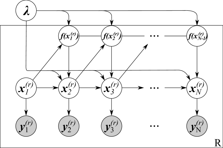
(a)

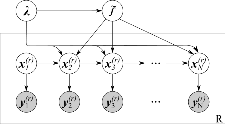
(b)

Figure 1: (a) Generative graphical model for a phase space with SDE-dynamics. (b) Generative model with inducing points compatible with SVI. Gray nodes represent observed variables and the plate notation indicates the repetition of random variables.

2.1 Inducing points as global variables for SVAE

The SGP approximation is built following [28]. Therefore, our inducing variables shall be the function points that result from evaluating $\bm{f}(\bm{x})$ at $m$ pseudo-inputs $\bm{\tilde{X}}=\{\bm{\tilde{x}}_{j}:\bm{\tilde{x}}_{j}\in\mathbb{R}^{d}\}_{j=1}^{m}$. We have noted the inducing points with uppercase to highlight that they are a collection of points in $\mathbb{R}^{d}$, and because we can arrange them as a matrix with $m$ rows and $d$ columns. Although a more general treatment is possible, for the sake of simplicity we assume that the $d$ GP s modeling the vector function $\bm{f}(\cdot)$ share the same set of pseudo-inputs. Since Equation (8) decomposes the equations of motion in $d$ independent equations, we shall study each component of $\bm{f}(\cdot)$ independently. The $i$-th component of the inducing points shall be noted as $\bm{\tilde{f}}_{i}=\{f_{i}(\bm{\tilde{x}}_{j}):\bm{\tilde{x}}_{j}\in\bm{\tilde{X}}\big{\}}$, and it is a vector of length $m$. From our previous assumptions, it follows that the $i$-th component of the inducing-points only depends on the values of the $i$-th GP. Furthermore, since $\bm{\tilde{f}}_{i}$ is derived from the same GP as $f_{i}(\cdot)$, the following conditional distribution holds:

$$\begin{bmatrix}f_{i}(\bm{x})\\ \bm{\tilde{f}}_{i}\end{bmatrix}\;|\lambda_{i}\sim\mathcal{N}\left(\begin{bmatrix}0\\ \bm{0}\end{bmatrix},\frac{1}{\lambda_{i}}\begin{bmatrix}\bm{K}_{i}(\bm{x},\bm{x})&\bm{K}_{i}(\bm{x},\bm{\tilde{X}})\\ \bm{K}_{i}(\bm{\tilde{X}},\bm{x})&\bm{K}_{i}(\bm{\tilde{X}},\bm{\tilde{X}})\\ \end{bmatrix}\right)\qquad i=1,2,\cdots,d,$$

where $\bm{x}\in\mathbb{R}^{d}$, $\bm{K}_{i}(\bm{x},\bm{x})$ is a $1\times 1$ matrix, and the matrices $\bm{K}_{i}(\bm{x},\bm{\tilde{X}})$, $\bm{K}_{i}(\bm{\tilde{X}},\bm{x})$ and $\bm{K}_{i}(\bm{\tilde{X}},\bm{\tilde{X}})$ should be read as the $1\times m$, $m\times 1$ and $m\times m$ matrices. Note that $f_{i}(\cdot)$ is a scalar function and it should not be confused with the $i$-th dimension of the inducing-points $\bm{\tilde{f}}_{i}$. The latter is the result of evaluating $f_{i}(\cdot)$ on a fixed set of points (the pseudo-inputs $\bm{\tilde{X}}$) and hence, it is possible to interpret it as a multivariate Gaussian random variable. The distribution of $f_{i}(\bm{x})$ conditioned on $\bm{\tilde{f}}_{i}$ and $\lambda_{i}$ can be written as

$$f_{i}(\bm{x})\mid\bm{\tilde{f}}_{i},\lambda_{i}\sim\mathcal{N}\bigg{(}f_{i}(\bm{x})\mid\bm{A}_{i}(\bm{x})\bm{\tilde{f}}_{i},\bm{P}_{i}(\bm{x})/\lambda_{i}\bigg{)}\qquad\text{with}$$ (15)

$$\bm{A}_{i}(\bm{x})=\bm{K}_{i}(\bm{x},\bm{\tilde{X}})\cdot\bm{K}_{i}^{-1}(\bm{\tilde{X}},\bm{\tilde{X}}),$$ (16)

$$\bm{P}_{i}(\bm{x})=\bm{K}_{i}(\bm{x},\bm{x})-\bm{K}_{i}(\bm{x},\bm{\tilde{X}})\cdot\bm{K}_{i}^{-1}(\bm{\tilde{X}},\bm{\tilde{X}})\cdot\bm{K}_{i}(\bm{\tilde{X}},\bm{x}).$$ (17)

Note that we have used a bold notation for $\bm{P}_{i}(\bm{x})$ because we compute its value through multiplications of matrices. However, the final $\bm{P}_{i}(\bm{x})$ from Equation (17) is a $1\times 1$ matrix and should be read as a scalar.

To “eliminate” the GP from the model shown in Figure 1(a), we need to replace the role of the conditional distribution involving the GP, $p(\bm{x}_{1:N}\mid\bm{f}(\cdot),\bm{\lambda},\bm{\theta})$, by the conditional distribution involving the inducing-points, $p(\bm{x}_{1:N}\mid\bm{\tilde{f}},\bm{\lambda},\bm{\theta})$. To that end, we lower bound the conditional distribution by using Jensen’s inequality (see, for example, [19]):

$$\log p(\{\bm{x}^{(r)}_{1:N}\}\mid\bm{\tilde{f}},\bm{\lambda},\bm{\theta}) =\log\mathbb{E}_{p(\bm{f}\mid\bm{\tilde{f}},\bm{\lambda},\bm{\theta})}\left[p(\{\bm{x}^{(r)}_{1:N}\}\mid\bm{f},\bm{\lambda},\bm{\theta})\right]$$ (18)

$$\geq\mathbb{E}_{p(\bm{f}\mid\bm{\tilde{f}},\bm{\lambda},\bm{\theta})}\log\left[p(\{\bm{x}^{(r)}_{1:N}\}\mid\bm{f},\bm{\lambda},\bm{\theta})\right]$$ (19)

$$\triangleq\log\tilde{p}(\{\bm{x}^{(r)}_{1:N}\}\mid\bm{\tilde{f}},\bm{\lambda},\bm{\theta}),$$ (20)

where we have reintroduced the superscript notation and used $\{\bm{x}^{(r)}_{1:N}\}$ as a shortcut for $\{\bm{x}^{(r)}_{1:N}\}_{r=1}^{R}$. Manipulating Equation (20) results in

$$\log\tilde{p}(\{\bm{x}^{(r)}_{1:N}\}\mid\bm{\tilde{f}},\bm{\lambda},\bm{\theta})=\sum_{r=1}^{R}\Big{(} \log p(\bm{x}^{(r)}_{1})+\sum_{t=1}^{N-1}\sum_{i=1}^{d}\log\mathcal{N}\left(x^{(r)}_{i,t+1}\mid x^{(r)}_{i,t}+\bm{A}_{i}(\bm{x}^{(r)}_{t})\bm{\tilde{f}}_{i},\lambda_{i}^{-1}\right)$$ (21)

$$-\frac{1}{2}\sum_{t=1}^{N-1}\sum_{i=1}^{d}\bm{P}_{i}(\bm{x}^{(r)}_{t})\Big{)},$$ (22)

where, just like in Equation (17), $\bm{P}_{i}(\bm{x}^{(r)}_{t})$ should be read as a scalar. A key property of Equation (22) is that it is written as a sum of R terms, each related to a different example $\bm{x}^{(r)}_{1:N}$. Following [31], we can use this lower bound in the SGP version of the original generative model as if it was $\log p(\{\bm{x}^{(r)}_{1:N}\}_{r=1}^{R}\mid\bm{\tilde{f}},\bm{\lambda},\bm{\theta})$, resulting in the graphical model shown in Figure 1(b). Note that the inducing variables work now as the global variables required by SVI. Therefore, we shall consider the graphical model from Figure 1(b) as our complete generative model.

2.2 Variational approximation to the SDE-based model

As usual with mean field variational inference, we start by breaking the posterior dependencies of the latent variables to achieve a tractable distribution:

$$p(\bm{x}_{1:N},\bm{\tilde{f}},\bm{\lambda},\bm{\theta},D\mid\bm{y}_{1:N})\approx q(\bm{x}_{1:N},\bm{\tilde{f}},\bm{\lambda},\bm{\theta},D)=q(\bm{x}_{1:N})q(\bm{\tilde{f}},\bm{\lambda},\bm{\theta})q(D).$$ (23)

We consider a simple mean field approximation that just factorizes the distributions distinguishing between the terms directly modeling the drift and diffusion, $\bm{\tilde{f}}$ and $\bm{\lambda}$, and other global variables $\bm{\theta}$:

$$q(\bm{\tilde{f}},\bm{\lambda},\bm{\theta})=q(\bm{\tilde{f}},\bm{\lambda}\mid\bm{\theta})q(\bm{\theta})\approx p(\bm{\tilde{f}},\bm{\lambda},\bm{\theta}\mid\bm{y}_{1:N}).$$ (24)

Note that the variational distributions of $\bm{\tilde{f}}$ and $\bm{\lambda}$ may be affected by $\bm{\theta}$. Think for example, in the length-scale parameters of the Gaussian kernels. To simplify the variational approximation, we take the variational factor $q(\bm{\theta})$ to be a Dirac distribution $q(\bm{\theta})=\delta_{\bm{\theta}^{*}}(\bm{\theta})$. Equation (24) becomes

$$q(\bm{\tilde{f}},\bm{\lambda},\bm{\theta})=q(\bm{\tilde{f}},\bm{\lambda}\mid\bm{\theta}^{*})\delta_{\bm{\theta}^{*}}(\bm{\theta}).$$ (25)

Since $p(\bm{f},\bm{\lambda}\mid\bm{\theta}^{*})$ was chosen as a conjugate prior in Equation (12), the optimal $q(\bm{\tilde{f}},\bm{\lambda}\mid\bm{\theta}^{*})$ is also in the same exponential family and therefore, it is the product of $d$ multivariate Gaussian-Gamma distributions:

$$\begin{split}q(\bm{\tilde{f}},\bm{\lambda}\mid\bm{\theta}^{*})=&\prod_{i=1}^{d}\mathcal{NG}(\bm{\tilde{f}}_{i},\lambda_{i}\mid\bm{\mu}_{i},\bm{\Sigma}_{i},\alpha_{i},\beta_{i}),\qquad\text{where}\\ \mathcal{NG}(\bm{\tilde{f}}_{i},\lambda_{i}\mid\bm{\mu}_{i},\bm{\Sigma}_{i},\alpha_{i},\beta_{i})\triangleq&\mathcal{N}(\bm{\tilde{f}}_{i}\mid\bm{\mu}_{i},\lambda_{i}^{-1}\bm{\Sigma}_{i})\cdot\Gamma(\lambda_{i}\mid\text{shape}=\alpha_{i},\text{rate}=\beta_{i}).\end{split}$$ (26)

Therefore, to find the variational approximation $q(\bm{\tilde{f}},\bm{\lambda}\mid\bm{\theta}^{*})$ we only need to determine which are the optimal parameters of the Gaussian-Gamma distributions. For the moment, let us assume that each $\bm{\tilde{f}}_{i}$ has well-defined variational parameters $[\bm{\mu}_{i},\bm{\Sigma}_{i},\alpha_{i},\beta_{i}]^{T}$, although in Section 2.3 we shall introduce a different parametrization.

After studying the variational approach to the SDE model, we can plug in Equation (25) into Equation (23) to find the complete variational approximation, which is

$$\begin{split}p(\bm{x}_{1:N},\bm{\tilde{f}},\bm{\lambda},\bm{\theta},D\mid\bm{y}_{1:N})&\approx q(\bm{x}_{1:N},\bm{\tilde{f}},\bm{\lambda},\bm{\theta},D)\\ &=q(\bm{x}_{1:N})q(\bm{\tilde{f}},\bm{\lambda},\bm{\theta})q(D)\\ &=q(\bm{x}_{1:N})q(\bm{\tilde{f}},\bm{\lambda}\mid\bm{\theta}^{*})\delta_{\bm{\theta}^{*}}(\bm{\theta})q(D).\end{split}$$

We can further simplify the variational approximation by assuming that the decoding parameters are singular $q(D)=\delta_{D^{*}}(D)$ and therefore

$$p(\bm{x}_{1:N},\bm{\tilde{f}},\bm{\lambda},\bm{\theta},D\mid\bm{y}_{1:N})\approx q(\bm{x}_{1:N})q(\bm{\tilde{f}},\bm{\lambda}\mid\bm{\theta}^{*})\delta_{\bm{\theta}^{*}}(\bm{\theta})\delta_{D^{*}}(D).$$ (27)

A key insight of the SVAE is that Equation (27) does not break the dependencies of $\bm{x}_{1:N}$ across time, which is intended to permit an accurate and flexible representation of the dynamics of state space [24]. In our case, since the state space is modeled through a SDE, the optimal factor graph $\bm{x}_{1:N}$ is a Markov chain. In order to help capturing the relevant dynamical information from $\bm{y}_{1:N}$ an encoding network is used. This permits obtaining probabilistic guesses of the latent vector $\bm{x}_{t}$ from the observation $\bm{y}_{t}$, introducing back-constraints that help in learning the dynamics.

To incorporate both the Markovian dynamics and the encoding information into the variational distribution $q(\bm{x}_{1:N})$, [24] proposes to parametrize it as a conditional random field. In our case, the conditional Markov field can be written as

$$q(\bm{x}_{1:N})\triangleq q(\bm{x}_{1:N},E) \propto\psi(\bm{x}_{1})\prod_{t=1}^{N-1}\psi(\bm{x}_{t},\bm{x}_{t+1})\prod_{t=1}^{N}\psi(\bm{x}_{t},\bm{y}_{t},E),$$ (28)

where the encoding potentials $\psi(\bm{x}_{t},\bm{y}_{t},E)$ are Gaussian factors whose means and covariances depend on $\bm{y}_{t}$ through an encoder neural network (note the mnemonic $E$). However, it is unrealistic to assume that this encoder will be able to output a good latent vector from a single measurement $\bm{y}_{t}$. What $\bm{y}_{t}$ lacks is the “context” of the time series (i.e., its previous and future samples), without which it would be impossible to extract the relevant dynamics.

A simple approach to tackle this issue that is connected with the dynamical systems theory would be as follows. Since we assume that $\bm{y}_{1:N}$ has been generated by some high-dimensional stationary dynamical system, we could build a delay embedding:

$$\bm{Y}_{t}=\Big{[}\bm{y}_{t}^{T},\bm{y}_{t-\tau}^{T},\dots,\bm{y}_{t-(l-1)\tau}^{T}\Big{]}^{T}\qquad\text{for }t=1+(l-1)\tau,2+(l-1)\tau,\dots,N,$$ (29)

where the vectors $\bm{y}_{t}$, $\bm{y}_{t-\tau}$, … are concatenated together in a single vector, and where $\tau$ and $l$ should be selected in such a way that the embedding contains all the information required for determining the future of the time series. Therefore, we could feed the encoder with $\bm{Y}_{t}$ (instead of $\bm{y}_{t}$) to calculate the phase state at time $t$. Furthermore, it is possible to automatize the construction of the delay embedding using a Convolutional Neural Network (CNN) or a RNN, as proposed in [22]:

$$\bm{Y}_{1:N}=\text{CNN}(\bm{y}_{1:N},E)\qquad\text{or}\qquad\bm{Y}_{1:N}=\text{RNN}(\bm{y}_{1:N},E).$$

Finally, it is also possible to combine all the methods together, e.g.  feeding the delay embedding into a CNN which then feeds a RNN. We experimentally found that feeding the delay embedding into the neural networks may be a valuable way of quickly initializing the state space.

Regardless of the specific encoding method, the resulting variational distribution for $q(\bm{x}_{1:N})$ now reads

$$q(\bm{x}_{1:N})\triangleq q(\bm{x}_{1:N},E) \propto\psi(\bm{x}_{1})\prod_{t=1}^{N-1}\psi(\bm{x}_{t},\bm{x}_{t+1})\prod_{t=1}^{N}\psi(\bm{x}_{t},\bm{Y}_{t},E).$$ (30)

2.3 Lower bound for SVI and learning phase

Lower bound

After selecting an approximation to the true posterior from some tractable family, variational inference tries to make this approximation as good as possible by reducing the inference procedure to an optimization problem in which the lower bound $\mathcal{L}$ of the marginal log-likelihood $\log p(\{\bm{y}^{(r)}_{1:N}\})$ is maximized. Hence, the description of the variational approximation cannot be complete without giving the lower bound $\mathcal{L}$. Furthermore, to explicitly write the lower bound allows us to highlight the role of $\tilde{p}(\bm{x}_{1:N}\mid\bm{\tilde{f}},\bm{\lambda},\bm{\theta})$ in our approximation (see Figure 1(b)). We lower bound $\log p(\{\bm{y}^{(r)}_{1:N}\})$ as

$$\begin{split}\log p(\{\bm{y}^{(r)}_{1:N}\})&\geq\mathbb{E}_{q(\{\bm{x}^{(r)}_{1:N}\},E)q(\bm{\tilde{f}},\bm{\lambda}\mid\bm{\theta}^{*})}\left[\log\Bigg{(}\frac{p(\{\bm{y}^{(r)}_{1:N}\}\mid\{\bm{x}^{(r)}_{1:N}\},D^{*})p(\{\bm{x}^{(r)}_{1:N}\}\mid\bm{\tilde{f}},\bm{\lambda},\bm{\theta}^{*})p(\bm{\tilde{f}},\bm{\lambda}\mid\bm{\theta}^{*})}{q(\{\bm{x}^{(r)}_{1:N}\},E)q(\bm{\tilde{f}},\bm{\lambda}\mid\bm{\theta}^{*})}\Bigg{)}\right]\\ &\geq\mathbb{E}_{q(\{\bm{x}^{(r)}_{1:N}\},E)q(\bm{\tilde{f}},\bm{\lambda}\mid\bm{\theta}^{*})}\left[\log\Bigg{(}\frac{p(\{\bm{y}^{(r)}_{1:N}\}\mid\{\bm{x}^{(r)}_{1:N}\},D^{*})\tilde{p}(\{\bm{x}^{(r)}_{1:N}\}\mid\bm{\tilde{f}},\bm{\lambda},\bm{\theta}^{*})p(\bm{\tilde{f}},\bm{\lambda}\mid\bm{\theta}^{*})}{q(\{\bm{x}^{(r)}_{1:N}\},E)q(\bm{\tilde{f}},\bm{\lambda}\mid\bm{\theta}^{*})}\Bigg{)}\right]\\ &\triangleq\mathcal{L},\end{split}$$ (31)

where we have substituted $p(\bm{x}_{1:N}\mid\bm{\tilde{f}},\bm{\lambda},\bm{\theta})$ by $\tilde{p}(\bm{x}_{1:N}\mid\bm{\tilde{f}},\bm{\lambda},\bm{\theta})$. Equation (31) can be arranged as

$$\mathcal{L}= \mathbb{E}_{q(\{\bm{x}^{(r)}_{1:N}\},E)}\left[\log p(\{\bm{y}^{(r)}_{1:N}\}\mid\{\bm{x}^{(r)}_{1:N}\},D^{*})\right]+\mathbb{E}_{q(\{\bm{x}^{(r)}_{1:N}\},E)}\left[\mathbb{E}_{q(\bm{\tilde{f}},\bm{\lambda}\mid\bm{\theta}^{*})}\left[\log\tilde{p}(\{\bm{x}^{(r)}_{1:N}\}\mid\bm{\tilde{f}},\bm{\lambda},\bm{\theta}^{*})\right]\right]$$ (32)

$$+\mathbb{H}\big{(}q(\{\bm{x}^{(r)}_{1:N}\},E)\big{)}-\mathcal{KL}\bigg{(}q(\bm{\tilde{f}},\bm{\lambda}\mid\bm{\theta}^{*})\mid p(\bm{\tilde{f}},\bm{\lambda}\mid\bm{\theta}^{*})\bigg{)},$$ (33)

where the second term can be written as

$$\mathbb{E}_{q(\bm{\tilde{f}},\bm{\lambda}\mid\bm{\theta}^{*})}\left[\log\tilde{p}(\{\bm{x}^{(r)}_{1:N}\}\mid\bm{\tilde{f}},\bm{\lambda},\bm{\theta}^{*})\right]=\sum_{r=1}^{R}\Bigg{[} \log p(\bm{x}^{(r)}_{1})+\sum_{t=1}^{N-1}\sum_{i=1}^{d}\log\mathcal{N}\left(x^{(r)}_{i,t+1}\mid x^{(r)}_{i,t}+\bm{A}_{i}(\bm{x}^{(r)}_{t})\bm{\bm{\mu}}_{i},\beta_{i}/\alpha_{i}\right)$$ (34)

$$-\frac{1}{2}\sum_{t=1}^{N-1}\sum_{i=1}^{d}\left[\bm{P}_{i}(\bm{x}^{(r)}_{t})+\text{tr}\left(\bm{A}_{i}(\bm{x}^{(r)}_{t})\bm{\Sigma}_{i}\bm{A}^{T}_{i}(\bm{x}^{(r)}_{t})\right)\right]$$ (35)

$$+\frac{N-1}{2}\sum_{i=1}^{d}\left[\psi^{0}(\alpha_{i})-\log(\alpha_{i})\right]\Bigg{]},$$ (36)

and where $\psi^{0}(\cdot)$ is the digamma function. Again, we highlight that a key property of the lower bound $\mathcal{L}$ is that it breaks as a sum of R terms, each corresponding to a single $\bm{y}^{(r)}_{1:N}$, which permits the use of mini-batches.

For a better understanding of how the lower bound leads to a proper reconstruction of the state space, we briefly discuss each of the terms of $\mathcal{L}$ from Equations (33) and (36). The first term from Equation (33) is basically measuring the expected reconstruction error (using a squared error) when decoding the phase space to predict $\bm{y}_{1:N}$. Therefore, the first term from Equation (33) is encouraging the decoder to fit as close as possible $\bm{y}_{1:N}$, given a variational distribution of the phase space, $\bm{x}_{1:N}$. This term may also influence the phase space itself. For instance, it may induce the separation of two points that lie close in the phase space, say $\bm{x}_{t_{1}}$ and $\bm{x}_{t_{2}}$, if they are decoded into two samples $\bm{y}_{t_{1}}$ and $\bm{y}_{t_{2}}$ with very different values.

The second term from Equation (36) is responsible for adjusting $\{\bm{A}_{i}(\bm{x}_{t})\}_{i=1}^{d}$ and $\{\bm{\mu}_{i}\}_{i=1}^{d}$ so that $x_{i,t+1}$ can be accurately predicted using $\bm{x}_{t}$. Furthermore, it also fits $\{\beta_{i}/\alpha_{i}\}_{i=1}^{d}$ to the variance of the residuals that result from these predictions. The third term from Equation (36) is more difficult to interpret. The terms $\{\bm{P}_{i}(\bm{x}_{t})\}_{i=1}^{d}$ come from Equation (17), and represent the uncertainty about the predictions of $f_{i}(\bm{x}_{t})$ using the inducing-points $\bm{\tilde{f}}$. Hence, Equation (36) encourages the minimization of these predictive uncertainties, which can be achieved by either tuning the hyperparameters of the kernel or changing the phase space (Note that $\{\bm{P}_{i}(\bm{x}_{t})\}_{i=1}^{d}$ depends on $\bm{x}_{t}$). The term involving $\big{\{}\text{tr}\big{(}\bm{A}_{i}(\bm{x}_{t})\bm{\Sigma}_{i}\bm{A}^{T}_{i}(\bm{x}_{t})\big{)}\big{\}}_{i=1}^{d}$ cannot be interpreted in isolation, since it would yield $\bm{\Sigma}_{i}\rightarrow\bm{0}$. This does not occur due to the Kullback-Leibler divergence from Equation (33), which tries to keep each of the $\bm{\Sigma}_{i}$ as close as possible to its prior value, say $\bm{\Sigma}_{i}^{(0)}$. Therefore, the maximization of $\mathcal{L}$ requires a compromise, which (usually) results in values of $\bm{\Sigma}_{i}$ comprised between $\bm{0}$ and $\bm{\Sigma}_{i}^{(0)}$. The fourth term from Equation (36) favours large values of $\alpha$, since $\psi(\alpha_{i})-\log(\alpha_{i})$ is strictly increasing for $\alpha_{i}>0$. This is consistent with the update rule of the Gaussian-Gamma posterior for Gaussians [32], where the $\alpha$ parameter is increased by $n/2$ after the observation of $n$ samples. In our setting, this could be problematic, since we shall repeatedly update the parameters while learning the distributions. Again, the solution $\alpha_{i}\rightarrow\infty$ is avoided by means of the Kullback-Leibler divergence from Equation (33).

We have highlighted the key influence of the Kullback-Leibler divergence for the parameters $\{\bm{\Sigma}_{i}\}_{i=1}^{d}$ and $\{\alpha_{i}\}_{i=1}^{d}$, but it also has an effect on the parameters $\{\bm{\mu}_{i}\}_{i=1}^{d}$ and $\{\beta_{i}\}_{i=1}^{d}$, forcing a compromise between fitting the data and the prior distribution. The last term from Equation (33) to be discussed is the entropy (third term). It helps preventing the optimization of $\mathcal{L}$ from simply placing high probability density where the prior does (a random walk process), since the entropy encourages to place probability everywhere it is possible.

Learning phase

Stochastic gradients can be used to learn both the variational distributions, the hyperparameters, and the encoding and decoding parameters. The computation of the gradients requires calculating the derivates of the lower bound from Equation (33). However, the first two expectation terms from Equation (33) are hard to compute. Consider, for example, the expectations of $\bm{A}_{i}^{(r)}(\bm{x}_{t}^{(r)})\bm{\mu}_{i}$ with respect to $q(\{\bm{x}^{(r)}_{1:N}\},E)$ which, depending on the kernel, may be even impossible to compute in closed form. To tackle this issue, a Monte Carlo approximation shall be used. This requires being able to generate samples from the state space $\bm{x}_{1:N}^{(r,s)}$ where $\bm{x}_{1:N}^{(r,s)}\sim q(\bm{x}^{(r)}_{1:N},E)\approx p(\bm{x}^{(r)}_{1:N}\mid~{}\bm{y}^{(r)}_{1:N})$. The superscript $(r,s)$ identifies one of the $S$ samples from the $r$-th observation used for the Monte Carlo approximation. Note that to be able to differentiate through the Monte Carlo approximation, the samples should keep the dependencies with the parameters $E$ of $q(\{\bm{x}^{(r)}_{1:N}\},E)$. This can be achieved through the reparametrization trick [33]. Hence, we shall use the notation for the samples as $\bm{x}_{1:N}^{(r,s)}(E)$. To draw samples from the phase space, we should first infer the optimal variational factors $q(\bm{x}_{1:N},E)$. The optimal variational distribution $q(\cdot)$ in a local mean field approximation can be found by taking expectations with respect to the other variational factors [19]. In our case, finding the variational factor $q(\bm{x}_{1:N},E)$ requires fixing the SDE parameters $\bm{\tilde{f}}$ and $\bm{\lambda}$, the hyperparameters $\bm{\theta}$ and the encoding potentials $\{\psi(\bm{x}_{t},\bm{y}_{t},E)\}_{t=1}^{N}$ before computing the expectation

$$\log q(\bm{x}_{1:N},E)\propto\mathbb{E}_{q(\bm{\tilde{f}},\bm{\lambda}\mid\bm{\theta}^{*})}\left[\log\tilde{p}(\bm{x}_{1:N}\mid\bm{\tilde{f}},\bm{\lambda},\bm{\theta}^{*})\right],$$ (37)

which permits identifying the following conditional Gaussian factors:

$$\begin{split}&\psi(\bm{x}_{1})=p(\bm{x}_{1}),\\ &\psi(\bm{x}_{t},\bm{x}_{t+1})=\mathcal{N}\big{(}\bm{x}_{t+1}\mid\bm{x}_{t}+\hat{\bm{\mu}}(\bm{x_{t}}),\text{diag}(\bm{\beta}/\bm{\alpha})\big{)}\qquad\text{with}\\ &\hat{\bm{\mu}}(\bm{x}_{t})=[\bm{A}_{1}(\bm{x}_{t})\bm{\mu}_{1},\bm{A}_{2}(\bm{x}_{t})\bm{\mu}_{2},\dots,\bm{A}_{d}(\bm{x}_{t})\bm{\mu}_{d}]^{T}\qquad\text{for }t=1,\dots,T-1,\end{split}$$ (38)

where the $\bm{A}_{i}$ has been defined in Equation (17), $\bm{\mu}_{i}$ is the $i$-th mean of the $i$-th Gaussian-Gamma distribution from $q(\bm{\tilde{f}},\bm{\lambda}\mid\bm{\theta}^{*})$, and $\bm{\alpha}$ and $\bm{\beta}$ are the result of stacking the $\{\alpha_{i}\}_{i=1}^{d}$ and $\{\beta_{i}\}_{i=1}^{d}$ parameters from this same distribution. According to Equation (38), we approximate the dynamics of the system as if it evolved following

$$\begin{split}&\bm{x}_{t+1}=\bm{x}_{t}+\hat{\bm{\mu}}(\bm{x}_{t})+\bm{w}_{t},\\ &\bm{w}_{t}\sim\mathcal{N}\big{(}\bm{0},\text{diag}(\bm{\beta}/\bm{\alpha})\big{)},\end{split}$$ (39)

where $\bm{w}_{t}$ plays the role of a random noise. Note that this variational model is analogous to any SSM. Therefore, it is possible to efficiently draw samples from $q(\{\bm{x}_{1:N}\})$ by using a forward filtering pass that collects information about the observations from the past; and then perform sampling in the backward pass, using at each node the conditional node potentials and combining them with the information from the past of the node [19, Section 17.4.3].

However, closed form solutions of the filtering and smoothing problems are only available for a few special cases. For example, the well-known Kalman filter provides the exact distributions for linear Gaussian systems [34]. In GP dynamical systems, where the transition dynamics are governed by Gaussian Processes (GPs), several approximations based on moment matching have been proposed [35, 36, 37]. Our solution uses the forward and backward passes described by [36, 37] which not only permits efficiently drawing samples from the chain, but also calculating the required statistics at each node. The main drawback with this approximation is this method only works when using squared exponential covariance functions as kernels [36, 37]. As an alternative method that enables the use of any kernel, we also implemented a particle filter, as suggested in [20].

After sampling the state space, a Monte Carlo approximation to the lower bound $\mathcal{L}$ can be computed. The gradients of the neural networks and the hyperparameters $\bm{\theta}$ can be calculated using automatic differentiation tools; in our implementation, we have used TensorFlow [38] and the GPflow library [39].

Finally, instead of using standard gradients, we exploit the exponential family conjugacy structure of the Gaussian-Gamma distributions to efficiently compute natural gradients with respect to the variational parameters. Indeed, the natural gradients can be computed explicitly for each dimension, which enables a fast update of the SDE parameters. We note with $\bm{\eta}^{(i)}$ the natural parameters of the $i$-th Gaussian-Gamma, which are

$$\bm{\eta}^{(i)}=\Big{[}\eta^{(i)}_{0},\eta^{(i)}_{1},\left(\bm{\eta}^{(i)}_{2}\right)^{T},\left(\bm{\eta}^{(i)}_{3}\right)^{T}\Big{]}^{T}=\Bigg{[}\alpha_{i}-\frac{1}{2},-\beta_{i}-\frac{\bm{\mu}_{i}^{T}\bm{\Sigma}_{i}^{-1}\bm{\mu}_{i}}{2},\bm{\mu}_{i}^{T}\bm{\Sigma}_{i}^{-1},\text{Vec}\Bigg{(}-\frac{\bm{\Sigma}_{i}^{-1}}{2}\Bigg{)}^{T}\Bigg{]}^{T},$$

where $\text{Vec}(\cdot)$ vectorizes the matrix $-\frac{\bm{\Sigma}_{i}^{-1}}{2}$ so that the natural parameters can be expressed as a vector. The natural gradients with respect to $\bm{\eta}^{(i)}$ are:

$$\tilde{\nabla}_{\bm{\eta}^{(i)}}\mathcal{L}= \left[(N-1)/2,-\sum_{r=1}^{R}\left[\Delta\bm{x}_{i}^{(r)}\right]^{T}\Delta\bm{x}_{i}^{(r)}/2,\sum_{r=1}^{R}\left[\Delta\bm{x}_{i}^{(r)}\right]^{T}\bm{A}_{i}^{(r)},-\text{Vec}\left(\sum_{r=1}^{R}\left[\bm{A}^{(r)}_{i}\right]^{T}\bm{A}_{i}^{(r)}\right)^{T}/2\right]^{T}$$ (40)

$$-\left(\bm{\eta}^{(i)}-\bm{\hat{\eta}}^{(i)}\right).$$ (41)

where $\bm{\hat{\eta}}$ are the prior natural parameters and we have noted for convenience $\Delta\bm{x}_{i}^{(r)}=\Delta\bm{x}^{(r)}_{i,1:(N-1)}$ and $\bm{A}_{i}^{(r)}=\bm{A}_{i}\left(\bm{x}^{(r)}_{1:(N-1)}\right)$. For a derivation of Equation (41) see Appendix A.

The resulting SDE-SVAE algorithm for computing the gradients is summarized in Algorithm 1 [24].

Algorithm 1 SVAE algorithm for SDE-based dynamics. To keep the notation uncluttered, we omit the indices that generate the sets, e.g,̇ we use $\{\psi(\bm{x}^{(r)}_{t},\bm{y}^{(r)}_{t},E)\}$ instead of $\{\psi(\bm{x}^{(r)}_{t},\bm{y}^{(r)}_{t},E)\}^{t=N,r=R}_{t=1,r=1}.$

1:A batch of experimental time series $\{\bm{y}^{(r)}_{1:N}\}$; the current variational parameters $\bm{\tilde{\eta}}$ and the hyperparameters $\bm{\theta^{*}}$ characterizing the distribution $q(\bm{\tilde{f}},\bm{\lambda},\bm{\theta}^{*})$; and the current weights of the encoder and the decoder, $E$ and $D^{*}$.

2:function compute_gradients($\{\bm{y}^{(r)}\}$, $\bm{\tilde{\eta}}$, $\bm{\theta}^{*}$, $D^{*}$, $E$)

3:     $\#$ Get the encoding potentials using the encoding network

4:      $\{\psi(\bm{x}^{(r)}_{t},\bm{y}^{(r)}_{t},E)\}\leftarrow$ NNet($\{\bm{y}_{1:N}^{(r)}\},E$)

5:      $\{\bm{\mu}_{i},\bm{\Sigma}_{i},\alpha_{i},\beta_{i}\}$ = unpack_Gaussian_Gamma_params($\bm{\tilde{\eta}}$)

6:     $\#$ Define the dynamic potentials using Equation (38)

7:     for all pairs $(r,t)$ do

8:          $\hat{\bm{\mu}}(\bm{x}^{(r)}_{t})\leftarrow[\bm{A}_{1}(\bm{x}^{(r)}_{t})\bm{\mu}_{1},\bm{A}_{2}(\bm{x}^{(r)}_{t})\bm{\mu}_{2},\dots,\bm{A}_{d}(\bm{x}^{(r)}_{t})\bm{\mu}_{d}]^{T}$

9:          $\psi(\bm{x}^{(r)}_{t},\bm{x}^{(r)}_{t+1})\leftarrow\mathcal{N}\Big{(}\bm{x}^{(r)}_{t+1}\mid\bm{x}^{(r)}_{t}+\hat{\bm{\mu}}(\bm{x}^{(r)}_{t}),\text{diag}(\bm{\beta}/\bm{\alpha})\Big{)}$

10:     end for

11:     $\#$ Draw $S$ samples from $q(\bm{x^{(r)}}_{1:N},E)$ and compute its entropy $\mathbb{H}\big{(}q(\bm{x}^{(r)}_{1:N},E)\big{)}$

12:     $\{\bm{\hat{x}}_{1:N}^{(r,s)}\}$, $\{\mathbb{H}\big{(}q(\bm{x}^{(r)}_{1:N},E)\}\leftarrow$ (      sample_and_get_entropy( $\{\psi(\bm{x}^{(r)}_{t},\bm{x}^{(r)}_{t+1},E)\},\{\psi(\bm{x}^{(r)}_{t},\bm{y}^{(r)}_{t},E)\}$ ) $\big{)}$

13:     $\#$ Compute lower bound with Equation (31)

14:      $\mathcal{L}$ = compute_L( $\{\bm{y}^{(r)}_{1:N}\},\{\bm{y}^{(r)}_{1:N}\},\{\mathbb{H}\big{(}q(\bm{x}^{(r)}_{1:N},E)\big{)}\},\{\bm{\mu}_{i},\bm{\Sigma}_{i},\alpha_{i},\beta_{i}\}$ )

15:     $\#$ Return gradients and natural gradients with Equation (41)

16:      return $\nabla_{D^{*},E,\bm{\theta}^{*}}\mathcal{L},\;\tilde{\nabla}_{\bm{\eta}}\mathcal{L}$

17:end function

3 Validation

In this section, we apply our model to a variety of experiments, to illustrate its potential to capture salient features of experimental time series. The experiments increase in complexity, and each of them tries to illustrate different aspects of the algorithm.

The experiments were run sharing a similar experimental setup. The encoder consisted of a single layer of 1D convolutions (with kernel size of 5 and 32 feature maps), followed by a single Gated Recurrent Unit (GRU) of size 64 and two Multilayer Perceptron (MLP) (one encoding the mean and the other one encoding the scale). The MLP used 128 hidden units with leaky-ReLu activations. The convolution layer was fed with five-dimensional delay embeddings, in which the time lag was selected using the average mutual information criterion. The delay embeddings were normalized before feeding them to the SDE-SVAE. We used both the moment matching algorithms and the particle filtering for drawing samples from the state space, but no significant differences in the final results were found. For illustrative purposes we show the moment matching results in the experiments from Sections 3.1 and 3.2, and the particle filter results in the experiments from Sections 3.3 and 3.4. The moment matching experiments used squared exponential kernels (as required by the algorithm) and the particle filter experiments used a Mattern $3/2$ kernel. The neural networks and the hyperparameters were optimized using the Adam optimizer with learning rate $3\cdot 10^{-4},$ whereas that the natural parameters were optimized using vanilla gradient descent with learning rate $0.1$.

3.1 Excited oscillator

We begin with a simple example in which a deterministic one-dimensional time series $\bm{y}_{1:N}$ oscillates while slowly increasing its amplitude. Specifically, we generated several realizations of the model using

$$\begin{split}y^{(r)}_{t}=\sqrt{2}\exp{\left(0.002\cdot t\right)}\cos\left(\frac{2\pi}{100}t+\phi^{(r)}\right),\qquad&r=1,2,\dots,120;\qquad t=1,2,\dots,500\end{split}$$ (42)

where $\phi^{(r)}$ is a random sample generated from a uniform distribution  $\mathcal{U}(0,2\pi)$. Note that this is the only source of randomness of the system. This time series is quite challenging for our model since the diffusion term should vanish to fit the deterministic equation generating the data ($\beta/\alpha\rightarrow 0$). However, the smoothness of the signal makes it easier to interpret the figures from the SVAE algorithm, making it a good illustrative example.

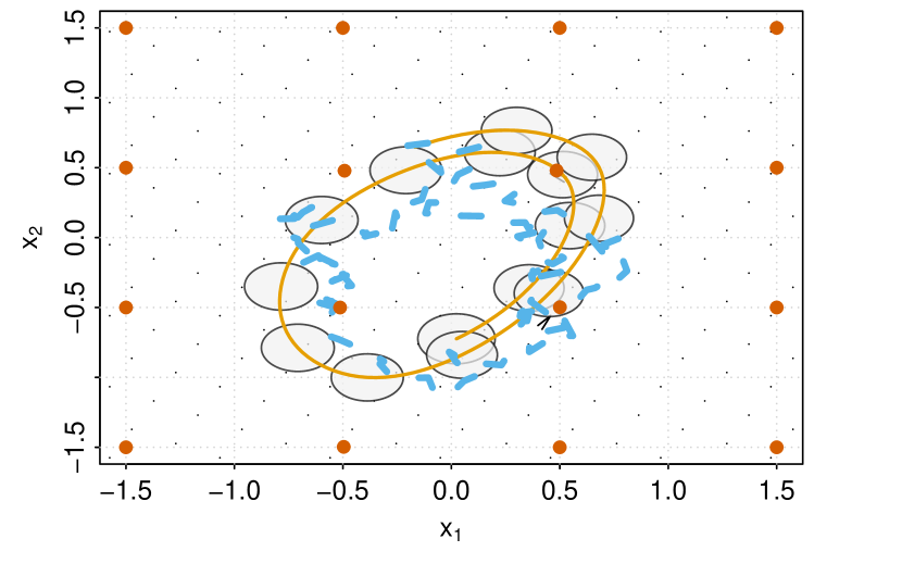
(a)

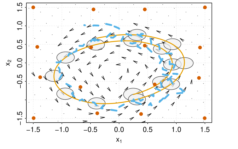
(b)

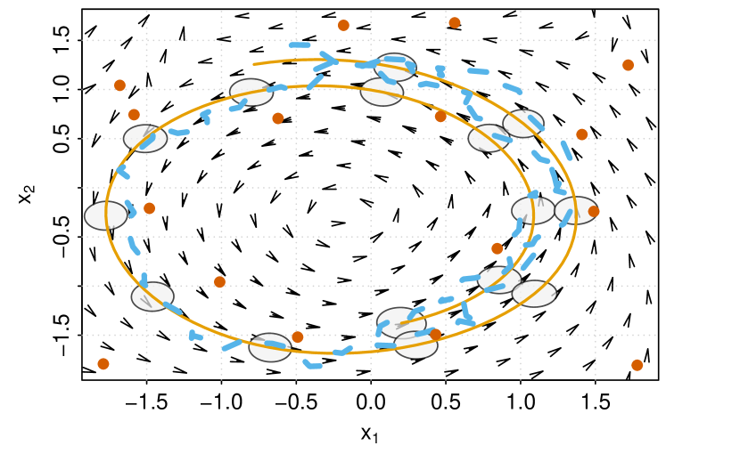
(c)

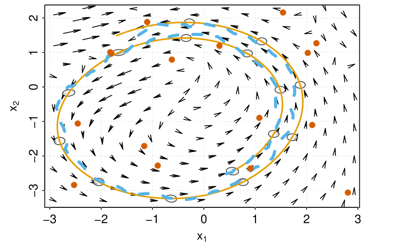
(d)

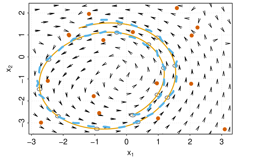
(e)

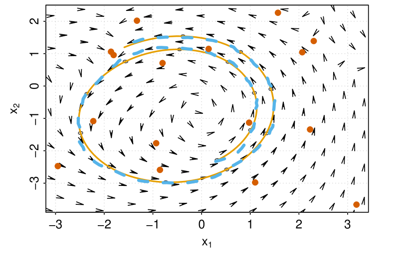
(f)

Figure 2: Evolution of the state space after (a) 35 iterations, (b) 131 iterations, (c) 323 iterations, (d) 1163 iterations, (e) 1847 iterations, and (f) 4247 iterations. The mean and covariances of the encoding network are represented by orange lines and gray ellipses, respectively. A single illustrative sample of the state space is shown with a dashed blue line. Finally, the pseudo-inputs are represented with reddish points, whereas the drift is represented by arrows.

Besides the choices for the neural networks described at the beginning of the section, the following parameters were selected. We used $d=2$ as dimension of the phase space; the size of the graph was set to $N=150$, effectively limiting the backpropagation through time to $150$ steps; the Monte Carlo approximations were calculated using $S=10$ samples; and $16$ inducing points were employed, initializing them after 5 epochs of training and scattering them into an uniform grid.

Figure 2 shows a small segment of the state space at several stages of the training procedure. Note that the state space shows the representation generated by the encoding network and the dynamics fitted by the SDE (Figure 2). A single illustrative sample of $\bm{x}_{1:N}$ is also shown. It is worth noting that the state space is able to capture the key features of the time series $\bm{y}_{1:N}$: the oscillatory pattern and the slow change in amplitude, therefore constructing a meaningful state space.

To confirm that the dynamics has been properly learned, we generate predictions from the SDE-SVAE given some small segment of data as input. This is illustrated in Figure 3(a). To generate a new prediction, the encoder creates a trajectory in state space for the given time series (colored in black, up to the vertical line). When the encoder runs out of input data, the last state of the encoded trajectory is used as the initial state of the fitted SDE. The SDE generates a new trajectory without the intervention of the encoder. Finally, the decoder maps the new phase space trajectories to the original space, generating new synthetic time series. Note that, since the SDE is a stochastic model, different trajectories may result from the same initial state. In Figure 3(a), two different synthetic time series are shown (in dashed-orange and solid-blue). Since the original time series is deterministic, the differences between both samples are small, although noticeable. This was expected, since the SDE-SVAE can not reach the limit $\beta/\alpha\rightarrow 0$, and therefore deterministic series are approximated with SDEs with a small diffusion term.

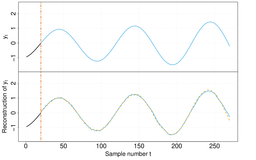
(a)

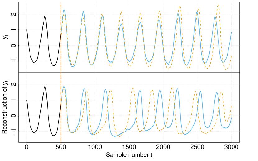
(b)

Figure 3: (a) Predictions from a SDE-SVAE for the excited oscillator. (b) Predictions from a SDE-SVAE for the Lotka-Volterra model. The top panels show real data; In (b), two different realizations of the synthetic data are shown, given the stochasticity of the model. The bottom panels show synthetic time series generated by the SVAE given the data up to the vertical line, colored in black.

3.2 Lotka-Volterra

In this section, we apply our SDE-SVAE to a nonlinear stochastic model inspired by the Lotka-Volterra equations. These equations are used in the study of biological ecosystems to describe the interactions between a predator and its prey. The diffusion approximation of the Lotka-Volterra model, described in [40, 41], is given by

$$\begin{split}\begin{bmatrix}dx_{1}(t)\\ dx_{2}(t)\end{bmatrix}=&\begin{bmatrix}{\alpha}x_{1}(t)-{\beta}x_{1}(t)x_{2}(t)\\ {\beta}x_{1}(t)x_{2}(t)-{\gamma}x_{2}(t)\end{bmatrix}\,\mathrm{d}t\\ &+\begin{bmatrix}{\alpha}x_{1}(t)+{\beta}x_{1}(t)x_{2}(t)&-{\beta}x_{1}(t)x_{2}(t)\\ -{\beta}x_{1}(t)x_{2}(t)&{\beta}x_{1}(t)x_{2}(t)+{\gamma}x_{2}(t)\end{bmatrix}^{1/2}\begin{bmatrix}dW_{1}(t)\\ dW_{2}(t)\end{bmatrix}.\end{split}$$ (43)

Note that the diffusion matrix does not meet the Lamperti transformation criteria from Equation (7). In this experiment we test how this affects the state space built by the SVAE.

We analyse the case $\alpha=30$, $\beta=0.2$ and $\gamma=18$. An illustrative portion of the real state space of the system is shown in Figure 4. The SVAE was fed with 10 different realizations of the $x_{1}(t)$ signal, sampled at 1000 Hz. Each of the resulting input signals, $y^{(r)}_{t}=x^{(r)}_{1}(t/1000)$ had a length of $600$ samples. We used $d=2$ for the state space dimension, $N=150$ for the size of the graphical model, $S=10$ for the number of Monte Carlo samples, and $m=10$ for the number of inducing points.

Figure 4 compares the true state space of the Lotka-Volterra system with the one obtained from the SDE-SVAE at the end of the training. Figure 3(b) shows predictions generated by a trained SDE-SVAE. Both figures illustrate the capability of the model to capture the most salient features of the system in state space and to generate credible synthetic signals despite the fact that the underlying model does not meet the Lamperti transformation criteria. However, the synthetic signals do not fully reproduce all the properties of the original system. For example, the variability of the height of the peaks is smaller in the synthetic signals, and they do not reach the most extreme values of the original signal.

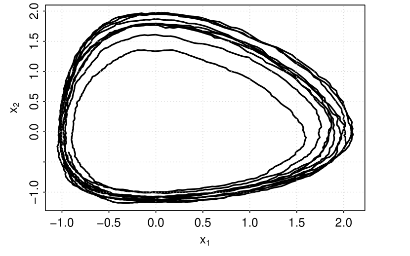
(a)

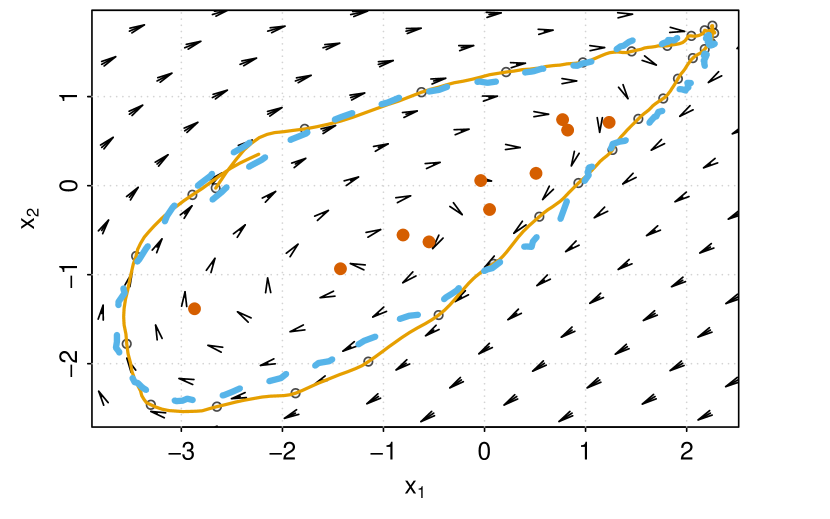
(b)

Figure 4: Comparison of the (a) true stochastic Lotka-Volterra state space and (b) the reconstructed one after 450 iterations. The meaning of the symbols from (b) is the same as in Figure 2.

3.3 Stochastic Rossler Model

In this section, we show a test where the SDE-SVAE did not perform well using a stochastic version of the Rossler system:

$$\begin{split}dx_{1}&=-(x_{2}-x_{3})dt+\delta\cdot dW_{1}(t),\\ dx_{2}&=(x_{1}+\alpha x_{2})+\delta\cdot dW_{2}(t),\\ dx_{3}&=(\beta+x_{3}(x_{1}-\gamma))dt+\delta\cdot dW_{3}(t),\end{split}$$ (44)

with $\alpha=0.2$, $\beta=0.2$, $\gamma=5.7$ and $\delta=0.1$. A representative portion of the real state space of the system is shown in Figure 5(a). The SVAE was fed with 200 different realizations of the $x_{1}(t)$ signal, which was sampled at 1000 Hz and chunked in segments of $100$ samples. We used $d=3$ for the state space dimension, $N=100$ for the size of the graphical model, $S=10$ for the number of Monte Carlo samples, and $m=64$ for the number of inducing points. The inducing points were initialized at the beginning of the training using a grid-based approach in the range $[-3,3]$.

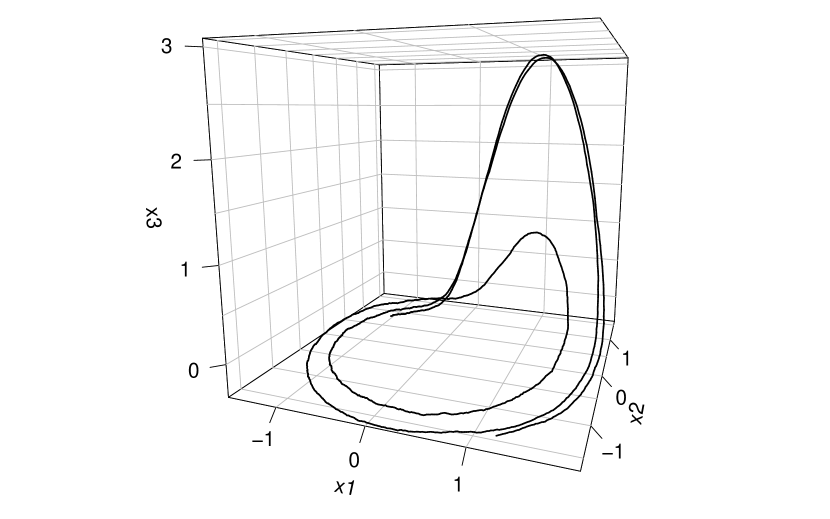
(a)

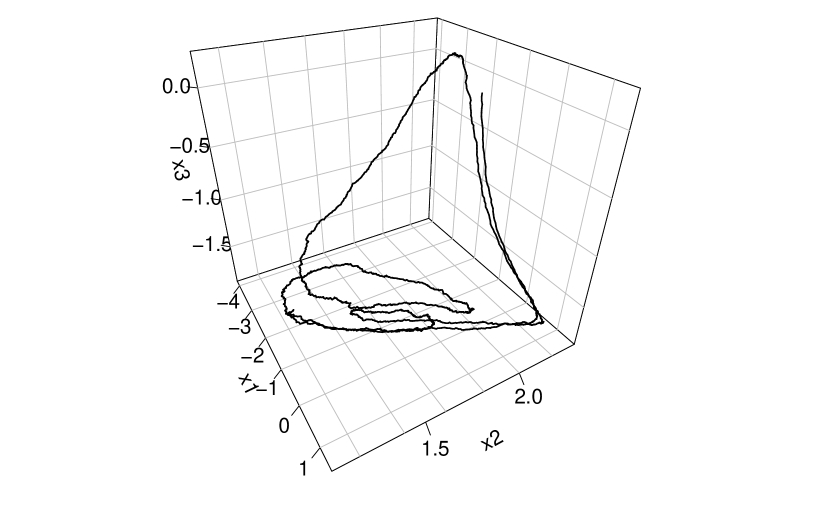
(b)

Figure 5: Comparison of the (a) true stochastic Rossler state space and (b) a reconstructed phase space after 5000 iterations and the observation of experimental data.

The real and synthetic state space are shown in Figures 5(a) and 5(b), respectively; the predictions generated after training the SDE-SVAE are shown in Figure 6(a). It is possible to visually assess that the state space from Figure 5(a) has a smaller diffusion than the state space from Figure 5(b). As a consequence, the synthetic reconstructions shown in Figure 6(a) aren’t as smooth as the real time series. Furthermore, the synthetic samples always decay to small amplitudes, without showing the rich dynamics of the original system. Clearly, the SDE-SVAE relied too heavily on the encoding network during training to reconstruct the state space which, despite the larger diffusion value, is reasonably disentangled. However, the drift function was not properly learned, which results in an overestimation of the diffusion and poor synthetic samples when the SDE-SVAE cannot rely on probabilistic guesses of the encoding network.

3.4 Stochastic Lorenz system

In this section, we study a stochastic version of the Lorenz system, a simplified model for the study of atmospheric convection:

$$\begin{split}dx_{1}&=\big{(}\sigma(x_{2}-x_{1})\big{)}dt+dW_{1}(t),\\ dx_{2}&=\big{(}x_{1}(\rho-x_{3})-x_{2}\big{)}dt+dW_{2}(t),\\ dx_{3}&=(x_{1}x_{2}-\beta x_{3})dt+dW_{3}(t).\end{split}$$ (45)

We focused on the values $\sigma=10,\beta=8/3,\rho=28$ which, in the case of the deterministic model, are known to produce chaotic behavior. A representative portion of the real state space of the system is shown in Figure 7(a). The SVAE was fed with 200 different realizations of the $x_{1}(t)$ signal, sampled at 1000 Hz. Each of the resulting input signals, $y^{(r)}_{t}=x^{(r)}_{1}(t/1000)$ had a length of $200$ samples. We used $d=3$ for the state space dimension, $N=200$ for the size of the graphical model, $S=10$ for the number of Monte Carlo samples, and $m=64$ for the number of inducing points. The inducing points were initialized at the beginning of training using a grid-based approach in the range $[-3,3]$.

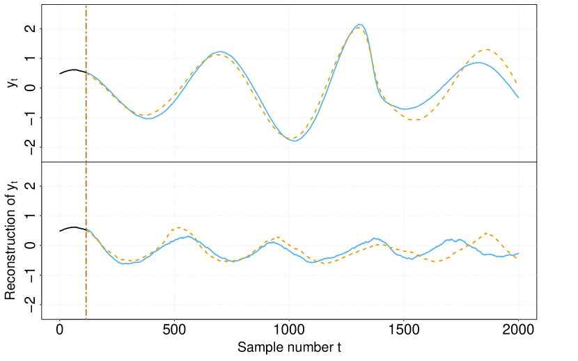
(a)

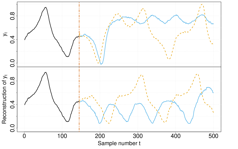
(b)

Figure 6: (a) Predictions from a SDE-SVAE for the Rossler model. (b) Predictions from a SDE-SVAE for the Lorenz model. The panel and symbols used in the Figure are the same as in Figure 3.

Figures 7(a) and 7(b) compare the real and a synthetic 3D-state space whereas that Figure 6(b) shows predictions generated by a trained SDE-SVAE. In Figure 7(b), it is possible to identify the two small elliptical trajectories (at the top-left and bottom right of the figure) as each of the lobes of the Lorenz attractor. The trajectories connecting both these regions represent transitions from one lobe to the other. Regarding Figure 6(b), the synthetic new series resemble the original ones. However, lobe transitions probabilities differ in the original and synthetic series. As an illustrative example, synthetic time series with sustained oscillations around $0.7$ (like the original blue one) were not observed. All synthetic time series performed only a few oscillations around $0.7$ before quickly transitioning to the other lobe (see the dashed-orange example in the lower panel of Figure 6(a)).

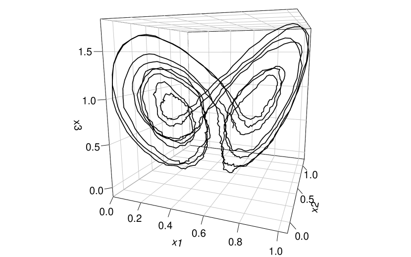
(a)

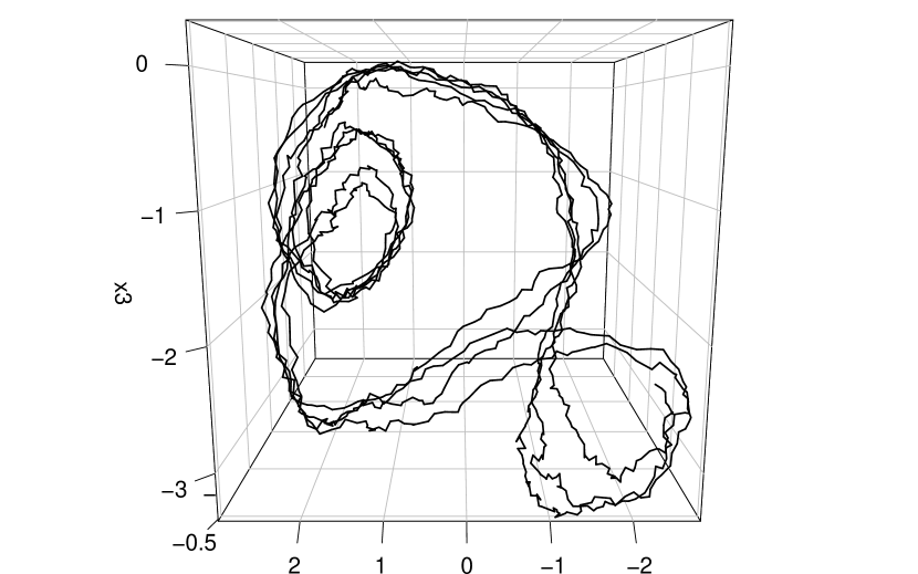
(b)

Figure 7: Comparison of the (a) true stochastic Lorenz state space and (b) a reconstructed phase space after 1000 iterations and the observation of experimental data.

4 Discussion and Conclusions

In this paper, we have introduced a method that permits simultaneously learning a Markovian representation of the data and its dynamics, which are assumed to be described by a SDE and hence represent the state space of the system. Therefore, our method enables to bridge the gap between experimental time series and the use of SDEs for modeling.

To this end, the SDE-SVAE uses a Bayesian approach that leverages graphical models, which impose the restriction of having SDE-like dynamics; and deep learning methods, which encodes probabilistic guesses which help in learning. Furthermore, SVAE takes advantage of SVI and natural gradients to implement an efficient inference algorithm, which permits the application of the method to large datasets that do not fit in main memory. From our point of view, the main contribution of this work is exploiting the great ability of machine learning to detect data patterns through a model that remains interpretable within a prominent paradigm of statistical physics. Indeed, the disentanglement of the dynamics in state space is achieved by only requiring that 1) similar state space vectors yield similar observed states, and 2) similar state space vectors result in similar dynamical evolution, described by a SDE.

The ability of the SDE-SVAE to capture the main dynamical features of the data and summarize them in the state space was shown using synthetic data. Although the results suggested that the SDE-SVAE is a powerful modeling tool, some drawbacks and future lines of work were also revealed.

A minor drawback of the method, which is shared with any technique using kernels, is that it requires a careful selection of a GP kernel that it is able to capture the relevant dynamics of the underlying process without loosing generalization capabilities. This is not always possible. For example, consider the use of the moment matching smoothing technique, which requires the use of squared exponential kernels. Although they may succeed in explaining the training data, the squared exponential kernels are only able to extrapolate around “small” regions around the inducing-points, where “small” is defined in terms of the length-scale hyperparameter. Hence, if a new experimental time series falls in a previously unexplored region of the state space, our technique will fail to predict the evolution of the system. It follows that, to improve the generalization properties of the drift estimates, we should endow the SDE-SVAE with the ability of using different kernels depending on the dynamical properties of the system under study. Indeed, sophisticated kernels are usually hand-crafted to enable pattern discovery and extrapolation in specialized applications [42].

An interesting difficulty when training the SDE-SVAE is that the autoencoder is trying to reconstruct a signal that is fed as input and that, unlike most autoencoders, the latent space is not a bottleneck since its dimension is larger than the input dimension. Luckily, the variational formulation does impose constraints on the latent space, difficulting overfitting. However, as shown in Section 3.3 with the Rossler model, overfitting is still possible even though we tried to use small encoder networks for preventing the network from memorizing the input data. A reformulation of the lower bound may be needed to permit the use of larger and deeper networks while, at the same time, completely avoid overfitting. For example, instead of reproducing the input time series, we may ask the SDE-SVAE to produce predictions several time steps ahead in the future. This may prevent overfitting and also places more emphasis in capturing the dynamics of the system.

Regarding the dynamics of the system, the experiments from Sections 3.2 and 3.4 also show that the SDE-SVAE does not fully reproduce all the relevant properties of the original time series. In the case of the Lotka-Volterra system, this is probably due to the fact that the system has a diffusion which is not compatible with the Lamperti transformation, which would permit its representation through SDEs with constant diffusions, as assumed by our model. Hence, the use of non-constant diffusions should be considered in future extensions of the model. This may also help in better capturing the properties of other systems. According to [8], deterministic dynamical systems with chaotic behaviour (such as the Lorenz system) may be accurately modeled as a linear system with a forcing term. In most regions of the state space the forcing is small. When this term is not negligible, it acts as a rare-event forcing that drives lobe switching and approximates the nonlinear dynamics of the system. This forcing term could be naturally incorporated into a non-constant diffusion of a SDE, which may help in capturing the properties of the system under study.

Another issue of the SDE-SVAE is the computational time it requires to build the state space when compared with simpler methods, like those based on lagged embeddings. While the latter are almost immediate, the SDE-SVAE may need hundreds or even thousands of iterations until convergence (just like any method involving neural networks). To alleviate this issue, an interesting line of work would be exploring initialization schemes that connect the efficient computation of lagged embeddings or Hankel-based embeddings with our method. Although in our experiments we fed the encoding network with lagged-embeddings, more sophisticated initialization schemes may accelerate convergence, facilitating the use of the SDE-SVAE in the analysis of experimental data. Note however that an advantage of the SDE-SVAE algorithm is that it is prepared for dealing with large datasets, whereas that most of the methods based on SVD are not.

Finally, it must be noted that the model proposed in this paper has room for improvement in light of the new advances in the field of machine learning. For example, [43, 44] recently introduced continuous-time latent variable models, which is the natural way of formulating physical systems and also permits handling irregularly sampled time series. Also, our model is based on the use of a variational posterior that factorizes the latent states ($\bm{x}$) and the drift function ($f(\cdot)$). More recently, several works started exploring the use of non-factorized posteriors [29, 30, 45], which may help in finding better embeddings and overcoming some of the issues found in the experimentation.

We believe that this work takes a valuable step towards developing an intuitive framework for building interpretable physical embeddings. To facilitate future research in this direction, we provide an open-source implementation of the method presented in this paper in [46].

Appendix A Closed form natural gradients

Let us consider the distribution of the inducing points $\bm{\tilde{f}}$ and the precision parameter $\lambda$ (inverse of the diffusion) of the SDE describing the evolution of the $i$-th component of the state space. According to Equation (12) the joint distribution of a finite set of drift points and the precision parameter is a Gaussian-Gamma distribution. The Gaussian-Gamma distribution can be written in the natural form as

$$\begin{split}\log q(\bm{\tilde{f}},\lambda,\mid\alpha,\beta,\bm{\mu},\bm{\Sigma})=&\begin{bmatrix}\alpha-\frac{1}{2}\\ -\beta-\frac{\bm{\mu}^{T}\bm{\Sigma}^{-1}\bm{\mu}}{2}\\ \bm{\Sigma}^{-1}\bm{\mu}\\ -\text{Vec}\big{(}\frac{\bm{\Sigma}^{-1}}{2}\big{)}\\ \end{bmatrix}^{T}\begin{bmatrix}\log\lambda\\ \lambda\\ \lambda\bm{\tilde{f}}\\ \lambda\text{Vec}(\bm{\tilde{f}}\bm{\tilde{f}}^{T})\end{bmatrix}+\\ &-\bigg{(}\log\Gamma(\alpha)-\alpha\log\beta-\frac{1}{2}\log\mid\bm{\Sigma}^{-1}\mid\bigg{)},\end{split}$$ (46)

or, in terms of the natural parameters

$$\bm{\eta}=\Big{[}\eta_{0},\eta_{1},\bm{\eta}_{2},\bm{\eta}_{3}\Big{]}^{T}=\Bigg{[}\alpha-\frac{1}{2},-\beta-\frac{\bm{\mu}^{T}\bm{\Sigma}^{-1}\bm{\mu}}{2},\bm{\mu}^{T}\bm{\Sigma}^{-1},\text{Vec}\Bigg{(}-\frac{\bm{\Sigma}^{-1}}{2}\Bigg{)}^{T}\Bigg{]}^{T},$$

as

$$\begin{split}\log q(\bm{\tilde{f}},\lambda,\mid\bm{\eta})\propto&\begin{bmatrix}\eta_{0}\\ \eta_{1}\\ \bm{\eta}_{2}\\ \bm{\eta}_{3}\\ \end{bmatrix}^{T}\begin{bmatrix}\log\lambda\\ \lambda\\ \lambda\bm{\tilde{f}}\\ \lambda\text{Vec}(\bm{\tilde{f}}\bm{\tilde{f}}^{T})\end{bmatrix}+\\ &-\bigg{(}\log\Gamma(\eta_{0}+1/2)-\big{(}\eta_{0}+1/2)\log\left(-\eta_{1}+\frac{\bm{\eta}_{2}^{T}\text{Mat}(\bm{\eta}_{3})^{-1}\bm{\eta_{2}}}{4}\right)-\frac{1}{2}\log\mid\text{Mat}(-2\bm{\eta_{3}})\mid\bigg{)}\\ =&\begin{bmatrix}\eta_{0}\\ \eta_{1}\\ \bm{\eta}_{2}\\ \bm{\eta}_{3}\\ \end{bmatrix}^{T}\begin{bmatrix}T_{0}(\tilde{\bm{f}},\lambda)\\ T_{1}(\tilde{\bm{f}},\lambda)\\ T_{2}(\tilde{\bm{f}},\lambda)\\ T_{3}(\tilde{\bm{f}},\lambda)\\ \end{bmatrix}-A(\bm{\eta})=\bm{\eta}^{T}\bm{T}(\tilde{\bm{f}},\lambda)-A(\bm{\eta}),\end{split}$$ (47)

where $\text{Mat}(\cdot)$ is the inverse of $\text{Vec}(\cdot)$ (i.e., it transforms a vector in a symmetric matrix), and $\bm{T}(\tilde{\bm{f}},\lambda)$ and $A(\bm{\eta})$ are the sufficient statistics and the log-partition of the Normal-Gamma distribution.

Our aim is to write now the lower bound from Equation (33) in terms of the natural parameters $\bm{\eta}$, also assuming that the prior can be written in terms of the natural parameters $\bm{\hat{\eta}}$, i.e.  $p(\bm{\tilde{f}},\lambda,\mid\bm{\hat{\eta}})$. To that end, it is useful the following property of the distributions with natural parameters [47]:

$$\mathbb{E}\left[T_{k}(\bm{\tilde{f}},\lambda)\right]=\nabla_{k}A(\bm{\eta}),$$ (48)

where $\nabla_{k}A(\bm{\eta})$ is a shortcut for $\nabla_{\bm{\eta}_{k}}A(\bm{\eta}).$ In the case of the Normal-Gamma distribution Equation (48) implies

$$\begin{split}\mathbb{E}\left[T_{0}(\bm{\tilde{f}},\lambda)\right]&=\mathbb{E}\left[\log\lambda\right]=\psi(\alpha)-\log\beta=\nabla_{0}A(\bm{\eta}),\\ \mathbb{E}\left[T_{1}(\bm{\tilde{f}},\lambda)\right]&=\mathbb{E}\left[\lambda\right]=\alpha/\beta=\nabla_{1}A(\bm{\eta}),\\ \mathbb{E}\left[T_{2}(\bm{\tilde{f}},\lambda)\right]&=\mathbb{E}\left[\lambda\bm{\tilde{f}}\right]=\frac{\alpha}{\beta}\bm{\mu}=\nabla_{2}A(\bm{\eta}),\\ \mathbb{E}\left[T_{3}(\bm{\tilde{f}},\lambda)\right]&=\mathbb{E}\left[\lambda\bm{\tilde{f}}\bm{\tilde{f}}^{T}\right]=\frac{\alpha}{\beta}\bm{\mu}\bm{\mu}^{T}+\bm{\Sigma}=\text{Mat}\left(\nabla_{3}A(\bm{\eta})\right).\end{split}$$ (49)

Using Equation (49) in Equations (33) and (36), and taking into account that $\bm{\tilde{f}}$ and $\lambda$ refer to a single dimension (the $i$-th dimension) of the SDE results in

$$\mathcal{L}(\bm{\eta})= \sum_{r=1}^{R}\Bigg{[}\sum_{t=1}^{N-1}\log\mathcal{N}\left(x^{(r)}_{i,t+1}\mid x^{(r)}_{i,t}+\bm{A}_{i}^{(r)}\bm{\bm{\mu}}_{i},\beta_{i}/\alpha_{i}\right)$$ (50)

$$-\frac{1}{2}\sum_{t=1}^{N-1}\left[\bm{P}_{i}(\bm{x}^{(r)}_{t})+\text{tr}\left(\bm{A}_{i}^{(r)}\bm{\Sigma}_{i}\left[\bm{A}_{i}^{(r)}\right]^{T}\right)\right]+\frac{N-1}{2}\left[\psi^{0}(\alpha_{i})-\log(\alpha_{i})\right]\Bigg{]}$$ (51)

$$-\mathcal{KL}\left[\bm{\eta}\mid\bm{\hat{\eta}}\right]+\text{constant}$$ (52)

$$= \left[\nabla_{0}A(\bm{\eta})\right]^{T}\frac{N-1}{2}-\frac{1}{2}\left[\nabla_{1}A(\bm{\eta})\right]^{T}\sum_{r=1}^{R}\left[\Delta\bm{x}_{i}^{(r)}\right]^{T}\Delta\bm{x}_{i}^{(r)}+\left[\nabla_{2}A(\bm{\eta})\right]^{T}\sum_{r=1}^{R}\left[\bm{A}_{i}^{(r)}\right]^{T}\Delta\bm{x}_{i}^{(r)}$$ (53)

$$-\frac{1}{2}\left[\nabla_{3}A(\bm{\eta})\right]^{T}\text{Vec}\left(\sum_{r=1}^{R}\left[\bm{A}^{(r)}_{i}\right]^{T}\bm{A}_{i}^{(r)}\right)-\mathcal{KL}\left[\bm{\eta}\mid\bm{\hat{\eta}}\right]$$ (54)

$$= \left[\nabla_{\bm{\eta}}A(\bm{\eta})\right]^{T}\left[(N-1)/2,-\sum_{r=1}^{R}\left[\Delta\bm{x}^{(r)}_{i}\right]^{T}\Delta\bm{x}_{i}^{(r)}/2,\sum_{r=1}^{R}\left[\Delta\bm{x}^{(r)}_{i}\right]^{T}\bm{A}_{i}^{(r)},-\text{Vec}\left(\sum_{r=1}^{R}\left[\bm{A}^{(r)}_{i}\right]^{T}\bm{A}_{i}^{(r)}\right)^{T}/2\right]^{T}$$ (55)

$$-\mathcal{KL}\left[\bm{\eta}\mid\bm{\hat{\eta}}\right],$$ (56)

where we have noted, to keep the notation uncluttered, $\Delta\bm{x}_{i}^{(r)}=\Delta\bm{x}^{(r)}_{i,1:(N-1)}$, $\bm{A}^{(r)}_{i}=\bm{A}_{i}\left(\bm{x}^{(r)}_{1:(N-1)}\right)$, and $\mathcal{KL}\left[\bm{\eta}\mid\bm{\hat{\eta}}\right]=\mathcal{KL}\left[q(\bm{\tilde{f}},\bm{\lambda}\mid\bm{\eta},\bm{\theta}^{*})\mid p(\bm{\tilde{f}},\bm{\lambda}\mid\bm{\hat{\eta}},\bm{\theta}^{*})\right].$

Given that the Kullback-Leibler divergence between two distributions with natural parameters can be written as

$$\mathcal{KL}\left[\bm{\eta}\mid\bm{\hat{\eta}}\right]=\left[\nabla_{\bm{\eta}}A(\bm{\eta})\right]^{T}\left(\bm{\eta}-\bm{\hat{\eta}}\right)-A(\bm{\eta})+A(\bm{\hat{\eta}}),$$

taking gradients in Equation (56) results in

$$\nabla_{\bm{\eta}}\mathcal{L}(\bm{\tilde{f}},\lambda)= \left[\nabla^{2}_{\bm{\eta}}A(\bm{\eta})\right]^{T}\left[(N-1)/2,-\sum_{r=1}^{R}\left[\Delta\bm{x}_{i}^{(r)}\right]^{T}\Delta\bm{x}_{i}^{(r)}/2,\sum_{r=1}^{R}\left[\Delta\bm{x}_{i}^{(r)}\right]^{T}\bm{A}_{i}^{(r)},-\text{Vec}\left(\sum_{r=1}^{R}\left[\bm{A}^{(r)}_{i}\right]^{T}\bm{A}_{i}^{(r)}\right)^{T}/2\right]^{T}$$ (57)

$$-\left[\nabla^{2}_{\bm{\eta}}A(\bm{\eta})\right]^{T}\left(\bm{\eta}-\bm{\hat{\eta}}\right).$$ (58)

Finally, and following [48], the natural gradients (noted with $\tilde{\nabla}$) can be computed using

$$\tilde{\nabla}\mathcal{L}(\bm{\eta})\triangleq\bm{F}_{\bm{\eta}}^{-1}\nabla\mathcal{L}(\bm{\eta}),$$ (59)

where $\bm{F}_{\bm{\eta}}$ is the Fisher information matrix. Furthermore, the Fisher information matrix of a member of the exponential family with natural parameters $\bm{\eta}$ is, according to [47],

$$\bm{F}(\bm{\tilde{\eta}})=\nabla^{2}_{\bm{\eta}}A(\bm{\eta}),$$ (60)

which applied to Equation (58) implies that

$$\tilde{\nabla}_{\bm{\eta}}\mathcal{L}=\left[(N-1)/2,-\sum_{r=1}^{R}\left[\Delta\bm{x}_{i}^{(r)}\right]^{T}\Delta\bm{x}_{i}^{(r)}/2,\sum_{r=1}^{R}\left[\Delta\bm{x}_{i}^{(r)}\right]^{T}\bm{A}_{i}^{(r)},-\text{Vec}\left(\sum_{r=1}^{R}\left[\bm{A}^{(r)}_{i}\right]^{T}\bm{A}_{i}^{(r)}\right)^{T}/2\right]^{T}-\left(\bm{\eta}-\bm{\hat{\eta}}\right).$$ (61)

References

- Takens [1981] F. Takens, Detecting strange attractors in turbulence, Lecture Notes in Mathematics 898 (1981) 366–381.
- Sauer et al. [1991] T. Sauer, J. A. Yorke, M. Casdagli, Embedology, Journal of statistical Physics 65 (1991) 579–616.
- Kantz and Schreiber [2004] H. Kantz, T. Schreiber, Nonlinear time series analysis, volume 7, Cambridge University Press, 2004.
- Vlachos and Kugiumtzis [2010] I. Vlachos, D. Kugiumtzis, Nonuniform state-space reconstruction and coupling detection, Physical Review E 82 (2010) 016207.
- Tran and Hasegawa [2019] Q. H. Tran, Y. Hasegawa, Topological time-series analysis with delay-variant embedding, Physical Review E 99 (2019) 032209.
- Press et al. [1991] W. H. Press, S. A. Teukolsky, B. P. Flannery, W. T. Vetterling, Numerical recipes in Fortran 77: volume 1, volume 1 of Fortran numerical recipes: the art of scientific computing, Cambridge university press, 1991.
- Schmid [2010] P. J. Schmid, Dynamic mode decomposition of numerical and experimental data, Journal of fluid mechanics 656 (2010) 5–28.
- Brunton et al. [2017] S. L. Brunton, B. W. Brunton, J. L. Proctor, E. Kaiser, J. N. Kutz, Chaos as an intermittently forced linear system, Nature communications 8 (2017) 1–9.
- Williams et al. [2015] M. O. Williams, I. G. Kevrekidis, C. W. Rowley, A data–driven approximation of the Koopman operator: Extending dynamic mode decomposition, Journal of Nonlinear Science 25 (2015) 1307–1346.
- Lusch et al. [2018] B. Lusch, J. N. Kutz, S. L. Brunton, Deep learning for universal linear embeddings of nonlinear dynamics, Nature communications 9 (2018) 1–10.
- Takeishi et al. [2017] N. Takeishi, Y. Kawahara, T. Yairi, Learning Koopman invariant subspaces for dynamic mode decomposition, in: Advances in Neural Information Processing Systems, 2017, pp. 1130–1140.
- Ayed et al. [2019] I. Ayed, E. de Bézenac, A. Pajot, J. Brajard, P. Gallinari, Learning dynamical systems from partial observations, arXiv preprint arXiv:1902.11136 (2019).
- Ouala et al. [2019] S. Ouala, D. Nguyen, L. Drumetz, B. Chapron, A. Pascual, F. Collard, L. Gaultier, R. Fablet, Learning latent dynamics for partially-observed chaotic systems, arXiv preprint arXiv:1907.02452 (2019).
- Raissi and Karniadakis [2018] M. Raissi, G. E. Karniadakis, Hidden physics models: Machine learning of nonlinear partial differential equations, Journal of Computational Physics 357 (2018) 125–141.
- Yap et al. [2014] H. L. Yap, A. Eftekhari, M. B. Wakin, C. J. Rozell, A first analysis of the stability of Takens’ embedding, in: Signal and Information Processing (GlobalSIP), 2014 IEEE Global Conference on, IEEE, 2014, pp. 404–408.
- Friedrich et al. [2011] R. Friedrich, J. Peinke, M. Sahimi, M. R. R. Tabar, Approaching complexity by stochastic methods: From biological systems to turbulence, Physics Reports 506 (2011) 87–162.
- Risken [1996] H. Risken, Fokker-planck equation, in: The Fokker-Planck Equation, Springer, 1996, pp. 63–95.
- Deisenroth and Rasmussen [2011] M. Deisenroth, C. E. Rasmussen, Pilco: A model-based and data-efficient approach to policy search, in: Proceedings of the 28th International Conference on machine learning (ICML-11), 2011, pp. 465–472.
- Murphy [2012] K. P. Murphy, Machine learning: a probabilistic perspective, MIT Press, 2012.
- Frigola et al. [2013] R. Frigola, F. Lindsten, T. B. Schön, C. E. Rasmussen, Bayesian inference and learning in Gaussian process state-space models with particle mcmc, in: Advances in Neural Information Processing Systems, 2013, pp. 3156–3164.
- Frigola et al. [2014] R. Frigola, Y. Chen, C. E. Rasmussen, Variational Gaussian process state-space models, in: Advances in neural information processing systems, 2014, pp. 3680–3688.
- Eleftheriadis et al. [2017] S. Eleftheriadis, T. Nicholson, M. Deisenroth, J. Hensman, Identification of gaussian process state space models, in: Advances in neural information processing systems, 2017, pp. 5309–5319.
- Krishnan et al. [2015] R. G. Krishnan, U. Shalit, D. Sontag, Deep Kalman filters, arXiv preprint arXiv:1511.05121 (2015).
- Johnson et al. [2016] M. Johnson, D. K. Duvenaud, A. Wiltschko, R. P. Adams, S. R. Datta, Composing graphical models with neural networks for structured representations and fast inference, in: Advances in Neural Information Processing Systems, 2016, pp. 2946–2954.
- Møller and Madsen [2010] J. K. Møller, H. Madsen, From state dependent diffusion to constant diffusion in stochastic differential equations by the Lamperti transform, DTU Informatics, 2010.
- Kloeden and Platen [1999] P. E. Kloeden, E. Platen, Numerical solution of stochastic differential equations, Applications of Mathematics, Springer, 1999.
- Ruttor et al. [2013] A. Ruttor, P. Batz, M. Opper, Approximate Gaussian process inference for the drift function in stochastic differential equations, in: Advances in Neural Information Processing Systems, 2013, pp. 2040–2048.
- García et al. [2017] C. A. García, A. Otero, P. Félix, J. Presedo, D. G. Márquez, Nonparametric estimation of stochastic differential equations with sparse Gaussian processes, Physical Review E 96 (2017) 022104.
- Ialongo et al. [2019] A. D. Ialongo, M. Van Der Wilk, J. Hensman, C. E. Rasmussen, Overcoming mean-field approximations in recurrent Gaussian process models, arXiv preprint arXiv:1906.05828 (2019).
- Curi et al. [2020] S. Curi, S. Melchior, F. Berkenkamp, A. Krause, Structured variational inference in partially observable unstable Gaussian process state space models, Proceedings of Machine Learning Research vol 120 (2020) 1–11.
- Hensman et al. [2013] J. Hensman, N. Fusi, N. D. Lawrence, Gaussian processes for big data, in: Uncertainty in Artificial Intelligence, 2013, p. 282.
- Murphy [2007] K. P. Murphy, Conjugate Bayesian analysis of the Gaussian distribution, Technical Report, 2007. URL: https://www.cs.ubc.ca/~murphyk/Papers/bayesGauss.pdf.
- Kingma and Welling [2013] D. P. Kingma, M. Welling, Auto-encoding variational Bayes, arXiv preprint arXiv:1312.6114 (2013).
- Kalman [1960] R. E. Kalman, A new approach to linear filtering and prediction problems, Journal of Basic Engineering 82 (1960) 35–45.
- Candela et al. [2003] J. Q. n. Candela, A. Girard, J. Larsen, C. E. Rasmussen, Propagation of uncertainty in Bayesian kernel models-application to multiple-step ahead forecasting, in: Proceedings of the IEEE International Conference on Acoustics, Speech, and Signal Processing, 2003 (ICASSP’03), volume 2, IEEE, 2003, pp. II–701.
- Deisenroth et al. [2009] M. P. Deisenroth, M. F. Huber, U. D. Hanebeck, Analytic moment-based Gaussian process filtering, in: Proceedings of the 26th Annual International Conference on Machine Learning, ACM, 2009, pp. 225–232.
- Deisenroth et al. [2012] M. P. Deisenroth, R. D. Turner, M. F. Huber, U. D. Hanebeck, C. E. Rasmussen, Robust filtering and smoothing with Gaussian processes, IEEE Transactions on Automatic Control 57 (2012) 1865–1871.
- TensorFlow Development Team [2015] TensorFlow Development Team, TensorFlow: Large-scale machine learning on heterogeneous systems, 2015. URL: https://www.tensorflow.org/, software available from tensorflow.org.
- De G. Matthews et al. [2017] A. G. De G. Matthews, M. Van Der Wilk, T. Nickson, K. Fujii, A. Boukouvalas, P. León-Villagrá, Z. Ghahramani, J. Hensman, GPflow: A Gaussian process library using TensorFlow, The Journal of Machine Learning Research 18 (2017) 1299–1304.
- Andrieu et al. [2010] C. Andrieu, A. Doucet, R. Holenstein, Particle Markov chain Monte Carlo methods, Journal of the Royal Statistical Society: Series B (Statistical Methodology) 72 (2010) 269–342.
- Boys et al. [2008] R. J. Boys, D. J. Wilkinson, T. B. Kirkwood, Bayesian inference for a discretely observed stochastic kinetic model, Statistics and Computing 18 (2008) 125–135.
- Wilson and Adams [2013] A. Wilson, R. Adams, Gaussian process kernels for pattern discovery and extrapolation, in: International Conference on Machine Learning, 2013, pp. 1067–1075.
- Chen et al. [2018] R. T. Q. Chen, Y. Rubanova, J. Bettencourt, D. K. Duvenaud, Neural ordinary differential equations, in: S. Bengio, H. Wallach, H. Larochelle, K. Grauman, N. Cesa-Bianchi, R. Garnett (Eds.), Advances in Neural Information Processing Systems 31, Curran Associates, Inc., 2018, pp. 6571–6583. URL: http://papers.nips.cc/paper/7892-neural-ordinary-differential-equations.pdf.
- Li et al. [2020] X. Li, T.-K. L. Wong, R. T. Chen, D. Duvenaud, Scalable gradients for stochastic differential equations, arXiv preprint arXiv:2001.01328 (2020).
- Doerr et al. [2018] A. Doerr, C. Daniel, M. Schiegg, D. Nguyen-Tuong, S. Schaal, M. Toussaint, S. Trimpe, Probabilistic recurrent state-space models, in: International Conference on Machine Learning (ICML), PMLR, 2018, pp. 1280–1289.
- García [2020] C. A. García, vaele: an SDE-based Structured Variational Autoencoder, https://github.com/constantino-garcia/vaele, 2020.
- DasGupta [2011] A. DasGupta, The exponential family and statistical applications, in: Probability for Statistics and Machine Learning, Springer, 2011, pp. 583–612.
- Amari [1998] S.-I. Amari, Natural gradient works efficiently in learning, Neural Computation 10 (1998) 251–276.