The specific star formation rate function at different mass scales and quenching: A comparison between cosmological models and SDSS

Abstract

We present the eddington bias corrected Specific Star Formation Rate Function (sSFRF) at different stellar mass scales from a sub-sample of the Sloan Digital Sky Survey Data Release DR7 (SDSS), which is considered complete both in terms of stellar mass (${\rm M_{\star}}$) and star formation rate (SFR). The above enable us to study qualitatively and quantitatively quenching, the distribution of passive/star-forming galaxies and perform comparisons with the predictions from state-of-the-art cosmological models, within the same ${\rm M_{\star}}$ and SFR limits. We find that at the low mass end (${\rm M_{\star}}=10^{9.5}-10^{10}\,{\rm M_{\odot}}$) the sSFRF is mostly dominated by star-forming objects. However, moving to the two more massive bins (${\rm M_{\star}}=10^{10}-10^{10.5}\,{\rm M_{\odot}}$ and ${\rm M_{\star}}=10^{10.5}-10^{11}\,{\rm M_{\odot}}$) a bi-modality with two peaks emerges. One peak represents the star-forming population, while the other describes a rising passive population. The bi-modal form of the sSFRFs is not reproduced by a range of cosmological simulations (e.g. Illustris, EAGLE, Mufasa, IllustrisTNG) which instead generate mostly the star-forming population, while a bi-modality emerges in others (e.g. L-Galaxies, Shark, Simba). Our findings reflect the need for the employed quenching schemes in state-of-the-art models to be reconsidered, involving prescriptions that allow “quenched galaxies” to retain a small level of SF activity (sSFR $=$ ${\rm 10^{-11}{\rm yr^{-1}}}$-${\rm 10^{-12}{\rm yr^{-1}}}$) and generate an adequate passive population/bi-modality even at intermediate masses (${\rm M_{\star}}=10^{10}-10^{10.5}\,{\rm M_{\odot}}$).

1 Introduction

In the last decade the observed star formation rates (SFRs) and stellar masses (${\rm M_{\star}}$) of galaxies have been extensively used to constrain and test theoretical models of galaxy formation. Cosmological simulations such as ANGUS (Tescari et al., 2014; Katsianis et al., 2015; García et al., 2017), Illustris (Vogelsberger et al., 2014), Horizon-AGN (Dubois et al., 2014; Volonteri et al., 2016), EAGLE (Schaye et al., 2015; Crain et al., 2015), Mufasa (Davé et al., 2017), IllustrisTNG (Pillepich et al., 2018) and SIMBA (Davé et al., 2019) have used sub-grid models to reproduce realistic galaxies in terms of stellar mass and SFR (Katsianis et al., 2017a; Davé et al., 2017; Zhao et al., 2020). In addition, semi-analytic models of galaxy formation such as L-GALAXIES (Henriques et al., 2015; Luo et al., 2016) and Shark (Lagos et al., 2018; Davies et al., 2019a) have given us the opportunity to study galaxy formation in larger volumes and be tested against stellar masses and SFRs at multiple redshifts. A useful metric, widely used in the literature to study both star formation and its efficiency is the Specific Star Formation Rate (sSFR) defined as ${\rm sSFR=SFR/M_{\star}}$. Hence, some authors have explored the number density of galaxies in bins of sSFRs namely the Specific Star Formation Rate Function (sSFRF, Ilbert et al., 2015; Davé et al., 2017; Katsianis et al., 2019). The sSFRF has advantages against median/average relations in 2d scatter plots which are not able to provide quantitative information of how galaxies are distributed and do not account for galaxies that could be under-sampled or missed by selection effects (Ilbert et al., 2015).

In order to study quenching in galaxies, it has been a common practice to study objects and their number distributions in terms of optical colors (Strateva et al., 2001), but a severe complication is that the latter strongly depend on the properties of the stellar population (e.g. metallicities, age distribution) and dust attenuation (Cantiello & Blakeslee, 2007; Li et al., 2007; Carter et al., 2009; Trayford et al., 2017; Bravo et al., 2020). This makes colors a less direct probe of the star formation activity of an object. Thus, in the last decade different studies have instead relied on the sSFR as a more direct probe of galaxy quenching (Darvish et al., 2018; Belfiore et al., 2018; Davies et al., 2019b). Furthermore, sSFRs have the advantage of being more easily comparable to the predictions of cosmological simulations.

When all galaxies are considered together (regardless of photometry, spectroscopy or morphology), the color distribution of galaxies can be approximated by the sum of two Gaussian functions, i.e. a bi-modal function (Baldry et al., 2008) with one representing star-forming objects and the other quenched galaxies. The sSFR is a property that directly relates with optical color, besides degeneracies due to dust attenuation, age and metallicity, so some authors expect or have found a similar color distribution as well. Santini et al. (2009) demonstrated that the sSFR of their sample from the GOODS-MUSIC catalog at ${\rm z\sim 0.3-2.5}$ shows a well-defined bi-modal distribution, with a clear separation between the actively star-forming objects and passive galaxies. In addition, Tzanavaris et al. (2010) showed a clear bi-modal sSFR distribution in their sample compiling UV data from the Swift UV/ Optical Telescope and mid-IR data from the Spitzer SpaceTelescope MIPS 24$\mu$m camera. Wetzel et al. (2012) using catalogs created from the SDSS survey (Abazajian et al., 2009), examined the sSFR distribution of satellite galaxies and its dependence on stellar mass, host halo mass, and halo-centric radius. The authors demonstrated that all galaxies, regardless of being central or satellites, exhibit a similar bi-modal sSFR distribution, with satellites being more likely to belong to the quenched population. Lenkić et al. (2016) suggested that the sSFRs in their sample constructed with Swift, Spitzer IRAC and MIPS 24 ${\rm\mu m}$ photometry of 183 galaxies in 46 compact groups, separate into two populations with one corresponding once again to the star-forming objects while the other to the quiescent galaxies. The authors demonstrated that galaxies in HI-rich groups tend to be MIR active, UV blue and have on average higher sSFRs, while galaxies residing in HI-poor groups populate the “low end of the sSFR distribution”. Davé et al. (2019) demonstrated that a bi-modal form emerges for the histograms of observed sSFRs obtained from the GALEX-SDSS-WISE Legacy CatalogS (GSWLC, Salim et al., 2016) and the Simba simulations.

In this work we use the Sloan Digital Sky Survey Data Release (SDSS) to construct specific Star Formation Rate Functions (sSFRFs) within different mass scales (section 2) from a sub-sample which is considered to have robust SFRs and stellar masses (has been compared successfully with other studies and SFR indicators) following Zhao et al. (2020). The objective is to study qualitatively the number density/distribution and quenching across different mass scales within strict SFRs and $\rm M_{\star}$ limits. We compare the observational constraints with the predictions from state-of-the-art cosmological models (section 3). In section 4 we present our conclusions.

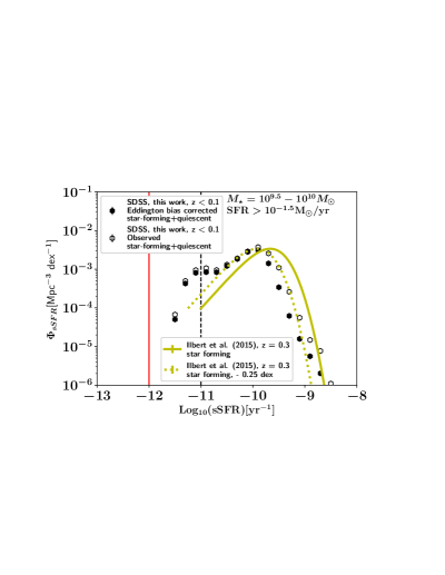
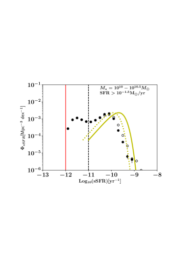
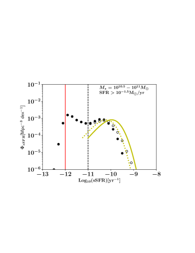
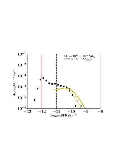
Figure 1: The black solid hexagons represent the Eddington bias corrected specific star formation rate function (sSFRF) at ${\rm z\sim 0}$ from the SDSS at mass intervals of $10^{9.5}-10^{10.0}\,{\rm M_{\odot}}$ (top left panel), $10^{10.0}-10^{10.5}\,{\rm M_{\odot}}$ (top right panel), $10^{10.5}-10^{11.0}\,{\rm M_{\odot}}$ (bottom left panel) and $10^{11.0}-10^{11.5}\,{\rm M_{\odot}}$ (bottom right panel). Open symbols represent the observed biased sSFRF. The black vertical line marks the limit of sSFR $=$ $10^{-11}{\rm yr^{-1}}$ with galaxies having lower values labelled as passive/quenched objects and galaxies having higher values labelled as star forming. For comparison we provide the observed sSFRs of Ilbert et al. (2015) which include only star forming objects, defined by a main sequence using a color-color selection) represented by the orange solid line and orange dotted line (shifted by -0.25 dex in order to consider systematics between star formation rate indicators). SDSS sSFRs $\leq 10^{-12}\,{\rm yr^{-1}}$ should only be considered as upper limits to the true values and we visualize this regime via the red vertical line.

2 The specific star formation rate function in SDSS at different mass scales

	${\rm Log_{10}(sSFR)}$ (${\rm yr^{-1}})$		$\phi_{\rm sSFR}\ \left({\rm Mpc}^{-3}\,dex^{-1}\ \right)$
		$10^{\,9.5-10}$ ${\rm M_{\odot}}$	$10^{\,10-10.5}$ ${\rm M_{\odot}}$	$10^{\,10.5-11}$ ${\rm M_{\odot}}$	$10^{\,11-11.5}$ ${\rm M_{\odot}}$
	-12.900000	-	-	-	1.38E-08 $\pm$ 1.17E-08
	-12.700000	-	-	-	4.84E-07 $\pm$ 1.23E-07
	-12.500000	-	-	9.75E-07 $\pm$ 3.25E-07	6.04E-06 $\pm$ 5.94E-07
	-12.300000	-	-	3.06E-05 $\pm$ 2.02E-06	6.60E-05 $\pm$ 2.41E-06
	-12.100000	-	-	5.29E-04 $\pm$ 1.74E-05	4.53E-04 $\pm$ 1.10E-05
	-11.900000	-	2.69E-04 $\pm$ 1.31E-05	1.59E-03 $\pm$ 5.01E-05	6.69E-04 $\pm$ 1.67E-05
	-11.700000	-	8.87E-04 $\pm$ 4.04E-05	1.31E-03 $\pm$ 3.81E-05	3.86E-04 $\pm$ 1.10E-05
	-11.500000	5.02E-05 $\pm$ 6.99E-06	1.15E-03 $\pm$ 5.47E-05	8.05E-04 $\pm$ 2.44E-05	2.13E-04 $\pm$ 6.11E-06
	-11.300000	4.27E-04 $\pm$ 4.06E-05	8.99E-04 $\pm$ 4.51E-05	6.19E-04 $\pm$ 1.85E-05	1.86E-04 $\pm$ 5.41E-06
	-11.100000	8.06E-04 $\pm$ 7.00E-05	6.99E-04 $\pm$ 3.45E-05	5.16E-04 $\pm$ 1.54E-05	1.99E-04 $\pm$ 5.34E-06
	-10.900000	8.40E-04 $\pm$ 7.38E-05	6.71E-04 $\pm$ 2.96E-05	5.28E-04 $\pm$ 1.38E-05	1.64E-04 $\pm$ 4.83E-06
	-10.700000	8.34E-04 $\pm$ 5.31E-05	8.40E-04 $\pm$ 3.23E-05	6.94E-04 $\pm$ 1.81E-05	1.25E-04 $\pm$ 3.46E-06
	-10.500000	1.21E-03 $\pm$ 7.88E-05	1.20E-03 $\pm$ 3.94E-05	8.83E-04 $\pm$ 2.24E-05	1.04E-04 $\pm$ 3.08E-06
	-10.300000	1.91E-03 $\pm$ 9.66E-05	1.88E-03 $\pm$ 5.88E-05	8.48E-04 $\pm$ 2.30E-05	8.21E-05 $\pm$ 2.87E-06
	-10.100000	2.81E-03 $\pm$ 1.29E-04	2.07E-03 $\pm$ 7.18E-05	5.09E-04 $\pm$ 1.45E-05	4.16E-05 $\pm$ 1.63E-06
	-9.900000	3.11E-03 $\pm$ 1.28E-04	1.03E-03 $\pm$ 3.95E-05	2.31E-04 $\pm$ 8.25E-06	1.70E-05 $\pm$ 9.72E-07
	-9.700000	1.41E-03 $\pm$ 8.18E-05	2.10E-04 $\pm$ 1.19E-05	6.26E-05 $\pm$ 3.09E-06	1.67E-06 $\pm$ 2.83E-07
	-9.500000	3.42E-04 $\pm$ 3.68E-05	4.42E-05 $\pm$ 4.64E-06	8.94E-06 $\pm$ 1.28E-06	4.26E-08 $\pm$ 4.26E-08
	-9.300000	6.20E-05 $\pm$ 1.21E-05	6.30E-06 $\pm$ 1.87E-06	7.35E-07 $\pm$ 3.85E-07	-
	-9.100000	1.57E-05 $\pm$ 7.74E-06	4.16E-06 $\pm$ 1.57E-06	-	-
	- 8.900000	5.58E-06 $\pm$ 3.37E-06	4.54E-07 $\pm$ 4.54E-07	-	-

Table 1: The Specific Star Formation Rate Function in the SDSS at mass bins of ${\rm M_{\star}}=10^{\,9.5-10}$ ${\rm M_{\odot}}$ (second column), ${\rm M_{\star}}=10^{\,10-10.5}$ ${\rm M_{\odot}}$ (third column), ${\rm M_{\star}}=10^{\,10.5-11}$ ${\rm M_{\odot}}$ (forth column) and ${\rm M_{\star}}=10^{\,10.5-11}$ ${\rm M_{\odot}}$ (fifth column).

The Sloan Digital Sky Survey Data Release 7 (SDSS DR7 Abazajian et al., 2009; Blanc et al., 2019; Concas et al., 2019; Zhao et al., 2020; Lu et al., 2020) is one of the most well-studied galaxy surveys at ${\rm z\sim 0}$. It provides stellar masses and SFRs for more than 500,000 galaxies which are based on the spectral distributions of Brinchmann et al. (2004), prescriptions for active galactic nuclei contamination and fiber aperture corrections following Salim et al. (2007). The SFRs are inferred from the Spectral Energy Distribution (SED) fitting of emission lines (predominately H${\rm\alpha}$), but in the cases of strong AGN contamination or no measurable emission lines, SFRs are obtained primarily using the 4000 ${\rm\AA}$ break. The stellar masses and SFRs described above have been used to estimate the local Galaxy Stellar Mass Function (GSMF, Baldry et al., 2008) and Star Formation Rate Function (SFRF, Zhao et al., 2020), respectively. The resulting distributions have been in agreement with a range of studies that employ different SFR indicators regardless of any shortcomings of SDSS. The GSMF and SFRF have been found to have confidence limits of $10^{9}$ ${\rm M_{\odot}}$ in terms of stellar mass (Weigel et al., 2016) and $10^{-1.5}$ ${\rm M_{\odot}/{\rm yr}}$ in terms of SFR (Zhao et al., 2020) so for our analysis we consider only objects within these strict ranges to construct the sSFRF. Given our adopted ${\rm M_{\star}}$ and SFR confidence limits, our sSFRFs are formally complete above ${\rm Log_{10}(sSFR)}>10^{-10.5}$ ${\rm yr^{-1}}$. Any incompleteness below these limits is coming from sources that are not present/observed in the SDSS main catalog. Thus, we caution the reader that any comparisons with the predictions from cosmological models should be done within the same ${\rm M_{\star}}$ and SFR limits. For this work we assume a Chabrier (2003) initial mass function and a Planck Collaboration et al. (2016) cosmology. We convert the stellar masses and SFRs from Kroupa (2001) to Chabrier (2003) by multiplying them by a factor of 1.063 following Bell (2003) and Madau & Dickinson (2014). For every galaxy, the sSFR is the SFR/${\rm M_{\star}}$ ratio so the initial values are unchanged. When necessary we shift the cosmology of other observations or simulations to Planck Collaboration et al. (2016) following Croton (2013).

We measure the sSFRFs in volume-limited samples that have been found complete in stellar mass and r-band luminosity (van den Bosch et al., 2008). In order to correct for the Malmquist bias caused by the nature of flux limit of the survey, we start with the observed sSFRFs computed via the 1/Vmax method (Li & White, 2009). The Vmax is calculated from the r-band Petrosian magnitude (K+E corrected to z=0.1), with also spectroscopy completeness taken into account. The observed distribution, due to the error on the sSFR estimation, suffers from the Eddington (1913) bias which we correct following Zhao et al. (2020). In short, without resort to assuming a functional form for the intrinsic (Eddington bias corrected) SFRFs and galaxy stellar mass functions, we correct the Eddington bias in both by subtracting the SFR/${\rm M_{\star}}$ of each galaxy using the average shift in the distributions induced by the bias. Then we employ the required corrections to the sSFRF. We start by convolving the SFRFs and GSMFs with SFR/${\rm M_{\star}}$ uncertainties taken from the assumption that each galaxy follows a Gaussian distribution around its median SFR/${\rm M_{\star}}$ and the uncertainty is the standard deviation. We obtain 1000 SFRs/${\rm M_{\star}}$ for each galaxy and then we build a histogram from the 1000 mock distributions (the median value of the resulting mocks). By doing this, we mimic the Eddington bias (EB) effect and create a double EB contaminated distribution. After comparing the latter with the observed SFRF in the x-axis, we interpolate and apply the necessary correction to the SFR of each galaxy in order to remove the Eddington bias. We then build another histogram which we convolve to generate a first order correction for the SFRF. We then again convolve the latter with the SFR uncertainties to obtain a first level Eddington bias corrected SFRF. If the latter distribution match the observed SFRF, it is implied that the above process should be enough to produce an intrinsic Eddington bias free SFRF. If not then we repeat the procedure by applying an additional correction N times, until the N-th order Eddingthon bias corrected SFRF converges to the observed distribution. For the SFRF and GSMF from the SDSS data only 2 iterations were necessary. The intrinsic SFRF (EB corrected) can then be found by applying these steps to the observed SFRFs/GSMFs. We then perform the corrections seen for the SFRF and GSMF to the specific star formation rates to obtain an Eddington bias corrected sSFRF.

The black solid hexagons of Fig. 1 represent the sSFRF at $z\sim 0$ from SDSS DR 7 at the stellar mass intervals of ${\rm M_{\star}}=10^{9.5}-10^{10.0}\,{\rm M_{\odot}}$ (top left panel), ${\rm M_{\star}}=10^{10.0}-10^{10.5}\,{\rm M_{\odot}}$ (top right panel), ${\rm M_{\star}}=10^{10.5}-10^{11.0}\,{\rm M_{\odot}}$ (bottom left panel) and ${\rm M_{\star}}=10^{11.0}-10^{11.5}\,{\rm M_{\odot}}$ (bottom right panel). The open symbols represent the observed Eddington biased sSFRF while the black vertical line labels the sSFR $=$ ${\rm 10^{-11}{\rm yr^{-1}}}$ limit which separates the passive/quenched objects and star forming objects. The above limit to separate the two populations is commonly adopted in the literature (Cassata et al., 2010; Tamburri et al., 2014; Katsianis et al., 2019; Matthee & Schaye, 2019; Thomas et al., 2019; Lovell et al., 2020) and is equivalent to the selection made by the NUV-r-J diagram Ilbert et al. (2013). At the same time it has the advantage of relating directly the separation of populations using a sSFR cut instead. We note that the applied Eddington bias correction does not change the form of the sSFRF. This is probably due to the cancellation of the Eddington bias that affects similarly both the star formation rate function and stellar mass function.

Starting from the low mass interval of ${\rm M_{\star}}=10^{9.5}-10^{10.0}\,{\rm M_{\odot}}$ we see that there is a peak of the distribution for objects with sSFRs of $10^{-10}{\rm yr^{-1}}$ pointing to the direction that most of the low-mass galaxies in our sample are still star forming. In addition, there is a second smaller peak with sSFR = $10^{-11}{\rm yr^{-1}}$. Moving to the mass interval of ${\rm M_{\star}}=10^{10.0}-10^{10.5}\,{\rm M_{\odot}}$ we demonstrate that the shape of the sSFR is bi-modal with two peaks at sSFR = ${\rm 10^{-10.2}{\rm yr^{-1}}}$ (representing star-forming galaxies) and sSFR = ${\rm 10^{-11.5}{\rm yr^{-1}}}$ (quiescent objects) suggesting that at these intermediate stellar masses there are numerous passive objects. At the more massive interval of ${\rm M_{\star}}=10^{10.5}-10^{11}\,{\rm M_{\odot}}$ (which represents objects with masses close to the characteristic stellar masses of the stellar mass function) we encounter once again a bi-modal form for the sSFRF, while the peak that represents quiescent objects (found at sSFR = ${\rm 10^{-11.9}{\rm yr^{-1}}}$) is slightly larger than that of star-forming galaxies (found at sSFR = ${\rm 10^{-10.5}{\rm yr^{-1}}}$). We note that both the star-forming and quenched peaks move towards lower sSFRs suggesting that as we move towards larger masses galaxies become more passive as a whole. High-mass galaxies tend to accumulate their stellar mass earlier than low-mass galaxies and thus on average be more passive (Fang et al., 2018). The above trend, called the sSFR downsizing phenomenon, has been widely seen in the literature (Cowie & Barger, 2008; Firmani & Avila-Reese, 2010; Twite et al., 2012; Hall et al., 2018). Last, at the high mass end (${\rm M_{\star}}=10^{11.0}-10^{11.5}\,{\rm M_{\odot}}$) we see the presence of a considerable star-forming population but most galaxies are quenched with the sSFRF having a peak at sSFR = ${\rm 10^{-11.9}{\rm yr^{-1}}}$.

We note that Wetzel et al. (2012) besides concluding that the distribution of sSFRs is bi-modal in SDSS argued that the high value and sharp peak of the low sSFRs at sSFR = ${\rm 10^{-12}{\rm yr^{-1}}}$ in their study, is partially driven by the limitation that low sSFR galaxies with no detectable emission lines are assigned SFRs mostly based on ${\rm D_{4000}}$. These are considered uncertain and usually upper limits (Feldmann, 2017) of the true values (i.e. there are a lot of objects that have artificial sSFRs $\sim$ ${\rm 10^{-12}{\rm yr^{-1}}}$). In addition, Hahn et al. (2019) emphasized that SDSS sSFRs $\leq 10^{-12}\,{\rm yr^{-1}}$ should only be considered as upper limits to the true values of sSFRs and we visualize this regime with the red vertical line of Fig. 1. We find that our peak related to the passive population has a lower amplitude than the one found by Wetzel et al. (2012) when we impose our strict ${\rm SFRs=10^{-1.5}}$ ${\rm M_{\odot}/{\rm yr}}$ cut . Furthermore, the peak associated to the quenched galaxies shifts slightly towards higher sSFRs with respect the parent sample which includes objects below the confidence limit. We demonstrate that the secondary peaks of the ${\rm M_{\star}}=10^{9.5}-10^{10}\,{\rm M_{\odot}}$ and ${\rm M_{\star}}=10^{10}-10^{10.5}\,{\rm M_{\odot}}$ (top right panel of Fig. 1) bins are found at $10^{-11}\,{\rm yr^{-1}}$ and $10^{-11.5}\,{\rm yr^{-1}}$, respectively. These are well above the $10^{-12}\,{\rm yr^{-1}}$ threshold value. In addition, the passive distribution of ${\rm M_{\star}}=10^{10.5}-10^{11}\,{\rm M_{\odot}}$ (bottom left panel of Fig. 1) with ${\rm sSFRs}<10^{-11.5}\,{\rm yr^{-1}}$ is enough to probe a non uni-modal distribution, without the need to involve any galaxies around ${\rm sSFRs}=10^{-12.0}\,{\rm yr^{-1}}$. Thus, we suggest that the bi-modality found in SDSS is robust within the SFR/mass limits adopted in our work. However, at the last mass bin where AGN contamination is expected to be important and SDSS SFRs are more uncertain, the peak value (${\rm sSFRs}=10^{-11.9}\,{\rm yr^{-1}}$) appears very close to the sSFR limit (${\rm sSFRs}=10^{-12}\,{\rm yr^{-1}}$) and could be indeed an artefact of the shortcomings discussed above. We have to note that our sub-sample is not a representative of the overall/total galaxy distribution. It instead represents galaxies with ${\rm SFRs>10^{-1.5}}$ ${\rm M_{\odot}/{\rm yr}}$ and ${\rm M_{\star}}>10^{9.0}\,{\rm M_{\odot}}$.

For comparison we show the observed sSFR of Ilbert et al. (2015) from the combined COSMOS and GOODS surveys which includes solely star-forming objects selected by a main sequence definition using a color-color selection) represented by the orange solid line and orange dotted line (shifted by -0.25 dex) of Fig. 1. We find that the star-forming peak given by Ilbert et al. (2015) is in good agreement with our results from SDSS within systematics between different SFR indicators (Katsianis et al., 2017b). Ilbert et al. (2015) suggested that the double-exponential and log-normal profiles provide good fits for their data with the double-exponential fit being more successful, especially at larger masses. The authors find that the shape of the sSFRF of objects highly depends on the mass, which we confirm in our work.

In conclusion, in Fig. 1 we show the bi-modal form of the SDSS sSFRF within the strict limits of ${\rm SFRs>10^{-1.5}}$ ${\rm M_{\odot}/{\rm yr}}$ and ${\rm M_{\star}>10^{9}}\,{\rm M_{\odot}}$. The shape of the distribution of sSFRs has been supported by previous studies based on other data-sets (Santini et al., 2009; Lenkić et al., 2016; Davé et al., 2019). In addition, we show how smoothly quenching is happening across different mass scales within these limits. Starting from the low-mass end, we demonstrate that most objects are star forming (being in excellent agreement with the double exponential form of the main sequence study of Ilbert et al.), but a small population that lies exactly at the limit of passive and star-forming objects arises (${\rm sSFRs}\sim 10^{-11}\,{\rm yr^{-1}}$). Moving to intermediate-mass objects, a passive population of galaxies with low specific star formation rates (${\rm sSFRs}\sim 10^{-11.5}\,{\rm yr^{-1}}$) starts emerging and it is abundant enough to give a bi-modal shape to the sSFRF. At the highest mass bins, the quenched population surpasses the star forming, though the latter is still significant. In table 2 we report the results from our analysis. The question that arises is: Are State-of-the-art cosmological models qualitatively in agreement with the observed sSFRF within the ${\rm SFR/M_{\star}}$ limits we adopted?

3 The sSFRF at different mass scales in cosmological models

3.1 Cosmological simulations and Semi-analytic models

In this work we explore a range of cosmological simulations. These assume various schemes, especially in terms of feedback prescriptions. The latter encloses the philosophy that is used from each group to quench galaxies and plays a major role in shaping the simulated objects, which otherwise would be extremely massive and star forming (Davé et al., 2011; Katsianis et al., 2015). We summarize the models considered below and in table 1:

	Run	L	NTOT	mDM	sSFRs Shift	Code	Feedback
		[Mpc]		[M⊙]	[dex]		(Ref)
	Illustris	106.5	$1820^{3}$	6.26$\times 10^{6}$	-0.3	AREPO	SNe: Winds, kinetic $+$ AGN: Radio mode-Mechanical, Quasar mode, Thermal/heating, radiation
	EAGLE	100	$1504^{3}$	9.70$\times 10^{6}$	+0.2	GADGET-3	SNe: Thermal/heating $+$ AGN: Thermal/heating
	Mufasa	73.5	$512^{3}$	9.70$\times 10^{7}$	-0.3	GIZMO	SNe: Winds-Kinetic $+$ AGN: Scheme to mimic Radio mode-heating
	IllustrisTNG	110.7	$1820^{3}$	7.5$\times 10^{6}$	-0.2	AREPO	SNe: Winds-kinetic $+$ AGN: Radio mode-Winds, Quasar mode-Thermal/heating
	Simba	148	$1024^{3}$	9.70$\times 10^{7}$	0 to -0.3	GIZMO	SNe: Winds-Kinetic $+$ AGN: Radio mode-Xray heating, Quasar mode-Winds and kinetic
	Shark	309.73	$1536^{3}$	2.21$\times 10^{8}$	- 0.3	GADGET-2	SNe: Winds-Kinetic $+$ AGN: Radio mode-heating
	ELUCID+L-Galaxies	694.4	$3072^{3}$	4.3$\times 10^{8}$	0 to + 0.1	L-GADGET	SNe: Heating, winds $+$ AGN: Radio mode-Thermal/heating, Quasar mode-Winds

Table 2: Summary of the different cosmological simulations used in this work. Column 1, run name; column 2, box size of the simulation in comoving Mpc; Column 3, total number of dark matter particles; Column 4 mass of the dark matter particle; Column 5, sSFR shift of the distribution needed to bring observed and simulated high star forming peaks to consonance; Column 6, code used; Column 7, combination of feedback implemented.

• Illustris (Genel et al., 2014; Vogelsberger et al., 2014) consists a cosmological simulation run with the moving-mesh code AREPO (Springel, 2010). Its sub-grid physics involve stochastic star formation, kinetic stellar feedback driven by SNe explosions, super-massive black hole (SMBH) growth and related AGN feedback since cosmological simulations lack the resolution to resolve all these phenomena. The free parameters ($>15$) are constrained by matching the results with the Cosmic Star Formation Rate density (CSFRD) evolution and the GSMF at $z\sim 0$ (Vogelsberger et al., 2013). SNe feedback is modelled in terms of galactic winds (Lopez et al., 2020) which employ an energy-driven scheme (Puchwein & Springel, 2013). The wind particles are launched in the neighborhood of stellar particles (Okamoto et al., 2010) and are kicked in a random directions, depositing their mass, momentum and thermal energy. In Illustris Black Holes (BHs) and AGN feedback rely on the implementations given by (Springel, 2005; Sijacki et al., 2007; Di Matteo et al., 2008). BHs are represented by collisionless, massive sink particles which grow in mass by accreting gas and merging with other BHs. Three different feedback processes emerge as a result of this growth including

  • thermal back reaction: a fraction of the energy released by the accreted gas couples thermally to nearby gas,

  • mechanical feedback: AGN jets inflate hot, buoyantly rising bubbles in the surrounding halo atmosphere,

  • electro-magnetic/radiative back reaction: the photo-ionisation and photo-heating rates of nearby plasma change due to the presence of the AGN radiation field.

  At high BH accretion rates (quasar-mode) thermal feedback is the dominant mechanism, while for low accretion rates (radio-mode) the mechanical feedback is important (Sijacki et al., 2008). The radiative feedback is most effective for accretion rates close to the Eddington limit but is considered weak compared to both thermal and mechanical feedback contributions (Vogelsberger et al., 2013). In addition, Sijacki et al. (2008) using cosmological simulations have found that the SFRs of galaxies are not sensitive to the nature of the bubble feedback.

• EAGLE (Schaye et al., 2015), run with an extended version of GADGET (Springel, 2005), adopts the stochastic thermal feedback scheme described in Dalla Vecchia & Schaye (2012). When a stellar particle reach the age of $3\times 10^{7}\,{\rm yr}$, it injects a spherical thermal input, increasing the internal energy of the neighboring particles and giving them a temperature jump $\Delta T$. This makes the available cold gas less and reduces star formation. The fraction ($f_{th,max}$) of the energy output is typically absorbed mostly by galaxies with low metallicities and high densities (Katsianis et al., 2017b). In addition to SNe feedback, EAGLE employs AGN feedback as well. Galaxies are seeded by BHs following Springel (2005), where seeds are placed at the center of every halo more massive than ${\rm M_{\star}}=10^{10}$ M${}_{\rm\odot}/h$ that does not already contain a BH. These grow by accretion of nearby gas particles or through mergers with other BHs. The gas accretion obeys the Bondi-Hoyle-Lyttleton formula following Rosas-Guevara et al. (2015) and assumes a radiative efficiency of $\epsilon_{r}=0.1$. This will stochastically heat neighboring particles (i.e. thermal feedback). AGN feedback by construction in EAGLE quench star formation in massive galaxies and is responsible for reproducing the high mass end of the stellar mass function (Furlong et al., 2015) and the super-massive black hole mass function (Rosas-Guevara et al., 2016). Cosmological simulations often make a distinction between ‘quasar’- and ‘radio-mode’ BH feedback (Croton et al., 2006a; Sijacki et al., 2008). The first occurs when the BH is accreting efficiently and comes in the form of a hot, nuclear wind, while the second operates when the accretion rate is low compared to the Eddington rate. EAGLE does not distinguish these two feedback modes unlike Illustris and its implementation is closer to a quasar-mode back reaction (Schaye et al., 2015). The rational behind this is to limit the number of feedback channels to the minimum required to match the observations. We note that Bower et al. (2017) showed that the AGN feedback in EAGLE keeps the surrounding gas heated. In this scheme a decreasing effectiveness of feedback from star formation leads to an increase in accretion into the black hole and thus black hole feedback will take over as star formation driven feedback fails to quench star formation. The above resembles a radio-mode back reaction instead of a quasar-mode behavior.

• Mufasa (Davé et al., 2017) uses a modified version of the code Gizmo (Hopkins, 2015), which relies on the GADGET-3 gravity solver. Stellar feedback is modelled using outflows in the form of decoupled two-phase winds relying on the Feedback In Realistic Environments (FIRE) zoom in simulations (Muratov et al., 2015). Thus, kinetic outflows are ejected with energy and momentum input to the intergalactic medium. The model allows hydrodynamical interactions and cooling of all gas at all times, unlike Illustris. To quench massive galaxies Mufasa follows the mass based quenching scheme given by Gabor & Davé (2012), in which a halo above a mass ${\rm M_{\rm quench}}=(0.96+0.48z)\times 10^{12}$ ${\rm M_{\odot}}$, maintains all halo gas at high temperature. This is intended to mimic the effects of the “radio mode” quenching that counteracts gas cooling and prevents star formation (Croton et al., 2006a; Bower et al., 2017).

• The IllustrisTNG (Pillepich et al., 2018) project is the successor of the Illustris simulations and includes an updated galaxy formation model with improvements to the SNe and AGN feedback (Weinberger et al., 2017) prescriptions in order to address some shortcomings of the original Illustris run. The above implementations included enhanced feedback, especially for objects with $10^{12}-10^{14}\,{\rm M_{\odot}}$ halo masses, Galactic Winds (GW) are injected this time isotropically, with larger wind, velocity and Energy Factors. So overall quenching is more efficient in IllustrisTNG than Illustris. This choice was driven by the fact that the last was unable to reproduce the $z<1$ star formation rate density, high mass end of stellar mass function at $z\sim 0$ and color bi-modality. For the case of the AGN feedback for high BH accretion rates relative to the Eddington limit, it is assumed that a fraction of the accreted rest mass energy heats the surrounding gas thermally. For low accretion rates a pure kinetic feedback component is used that inputs momentum to the surrounding gas in a stochastic manner. A key difference with the original Illustris model is that the radio bubble feedback for low accretion rates is replaced by kinetic winds.

• Simba (Davé et al., 2019) is the successor of Mufasa. The employed metal-loaded winds rely on Muratov et al. (2015) and Anglés-Alcázar et al. (2017a). The most significant improvement is that instead of the mass quenching feedback scheme (Gabor & Davé, 2012), BHs are included, seeded and grown. There are two channels for BH accretion: a Torque-limited component from cold gas and a Bondi component from hot gas. The resulting energy from the above process (Anglés-Alcázar et al., 2017b) is used to drive feedback that quenches galaxies. The above is modeled via kinetic bi-polar outflows and X-ray heating. The kinetic feedback component kicks for high Eddington ratios in which AGN drive galactic winds with velocities of $\sim 1000$ km/s (Perna et al., 2017). The X-ray heating back reaction is modeled by a jet mode in which AGN drive hot gas that heats the surrounding gas (Fabian, 2012) for objects with low Eddington ratios. This way the observed dichotomy in BH growth is achieved (Perna et al., 2017). X-ray feedback is modeled by heating from black holes following the scheme introduced by Choi et al. (2012). According to Davé et al. (2019) this heating has a minimal effect on the galaxy mass function, but provides an important factor to fully quench massive galaxies. In short, the AGN model employed in SIMBA has some similarities to the two-mode thermal/kinetic AGN feedback model employed in Illustris-TNG. However, there are some key differences like the fact that Illustris-TNG uses a spherical thermal back-reaction at high Eddington ratios, while Mufasa employs a kinetic feedback.

We have to note that cosmological simulations, like the ones discussed above, are computationally expensive since they involve both dark matter and gas elements/particles. This makes them restricted in terms of resolution (thus, are uncertain at the low mass end) and box-size (thus, have limited statistics for massive objects). Another limitation is that the parameters of the models that describe star formation and feedback depend highly on resolution (Zhao et al., 2020) and usually there is no convergence between different resolutions (Schaye et al., 2015). Thus, it is debatable if any of these models are actually physical or they have the “ideal” combination of parameters for the adopted resolution in order to re-produce key observables like the GSMF. On the other hand, semi-analytic models (SAMs) use pre-calculated dark matter merger trees from N-body simulations and follow the formation of galaxies with simplified and observationally motivated, analytic prescriptions (Hirschmann et al., 2012; Lagos et al., 2018). Since SAMs are less computationally expensive in the construction of galaxy samples, they can achieve much better statistics (by orders of magnitude) compared to those from cosmological hydrodynamical simulations. In our work we employ the following semi-analytic models:

• The ELUCID simulation (Wang et al., 2016) traces $3072^{3}$ dark matter particles in a periodic box of 644 Mpc. The N-body simulation was run with L-GADGET, a memory-optimized version of GADGET-2. It is constrained (in terms of initial conditions) by the re-constructed initial density field of SDSS DR 7 (Wang et al., 2014). ELUCID has been used to study galaxy quenching (Wang et al., 2018), galaxy intrinsic alignment (Wei et al., 2018) and cosmic variance (Chen et al., 2019) while it was also combined with an abundance matching method to evaluate galaxy formation models (Yang et al., 2018). In our work, we combine the merger trees taken from the ELUCID N-body simulations with the L-Galaxies Semi Analytic Model (SAM, Luo et al., 2016). Galaxies are assumed to form at the centers of the dark matter haloes while the recipes that describe physical baryonic processes (e.g. star formation and metal production, SNe feedback, black hole growth and AGN feedback) are implemented by the SAM (Fu et al., 2010; Fu et al., 2013). The parameters are constrained by the observed galaxy stellar and HI (neutral hydrogen) and H2 (molecular hydrogen ) mass functions at $z=0$. SNe feedback decreases the SFRs of the low mass objects by heating and ejecting the available gas within the halo (Fu et al., 2013), while the AGN model (Croton et al., 2006a) is extremely efficient in switching off cooling in massive haloes. Some advantages of this model is that it is resolution independent (with successful convergence results for satellites in massive haloes), while it includes environmental effects like cold gas stripping.

• The Shark semi-analytic model (Lagos et al., 2018) is merged with the Synthetic UniveRses For Surveys (SURFS) simulation of $1536^{3}$ dark matter particles in a periodic box of 310 Mpc (Elahi et al., 2018). The N-body simulation was run with a memory-optimized version of GADGET-2 for a $\Lambda$CDM cosmology. The reference simulation uses a Planck cosmology (Planck Collaboration et al., 2016) and sample scales and halo masses down to 1 kpc and ${\rm M_{\star}}=10^{8}\,{\rm M_{\odot}}$, respectively. The haloes are tracked and identified with a state-of-the-art 6D halo finder and merger tree builder (Elahi et al., 2019). Shark includes several processes such as gas cooling (Croton et al., 2006b), stellar feedback (Lagos et al., 2013; Muratov et al., 2015) in terms of galactic winds/outflows that escape either the host galaxy or the halo, radio-mode AGN feedback (Croton et al., 2016) in the form of gas heating and star formation (Krumholz, 2013). The parameters of the model were constrained from the $z=0$, 1, 2 stellar mass functions, the z = 0 black hole-bulge mass relation and the stellar mass vs size relation. Bravo et al. (2020) showed that Shark reproduces well the color bi-modality, though the transition from predominantly star-forming galaxies to passive objects happens at stellar masses that are larger than the ones found by the GAMA observations.

We have to note that in SAMs, unlike cosmological simulations, the dynamics of the baryonic component (gas and stars) and their interaction with dark matter are not followed directly. This is one of the main disadvantages of SAMs which use analytical prescriptions to model the above (Benson & Bower, 2011; Hirschmann et al., 2012). In SAMs we are forced to make strong assumptions about the geometry and dynamics of gas, while they are unable to probe details for the galaxy and halo structure. Hydrodynamic simulations can compensate for this limitation and investigate the resolved properties of galaxies (like the gas-phase metallicity, SFR and stellar mass distributions) within galaxies, at the expense of being computationally expensive. In our work we focus on the galaxy sSFRF (i.e. integrated SFRs and integrated stellar masses of galaxies) and thus SAMs, with their unparalleled statistics and large volumes can provide powerful tools to investigate the sSFR distribution.

In conclusion, both SAMs and hydrodynamical simulations are forced to implement uncertain models that involve numerous parameters to approximate star formation or feedback from SNe and AGN, with SAMs having the advantage of better statistics in larger volumes, while simulations having the advantage that they follow gas dynamics and do not need to employ analytic prescriptions to do so. There are differences and similarities between different collaborations. Some concordances of great importance are that they tuned the parameters of their models to the observed $z\sim 0$ GSMF while SNe feedback decreases SFRs in low-mass objects and AGN is tuned to quench galaxies at the high-mass end.

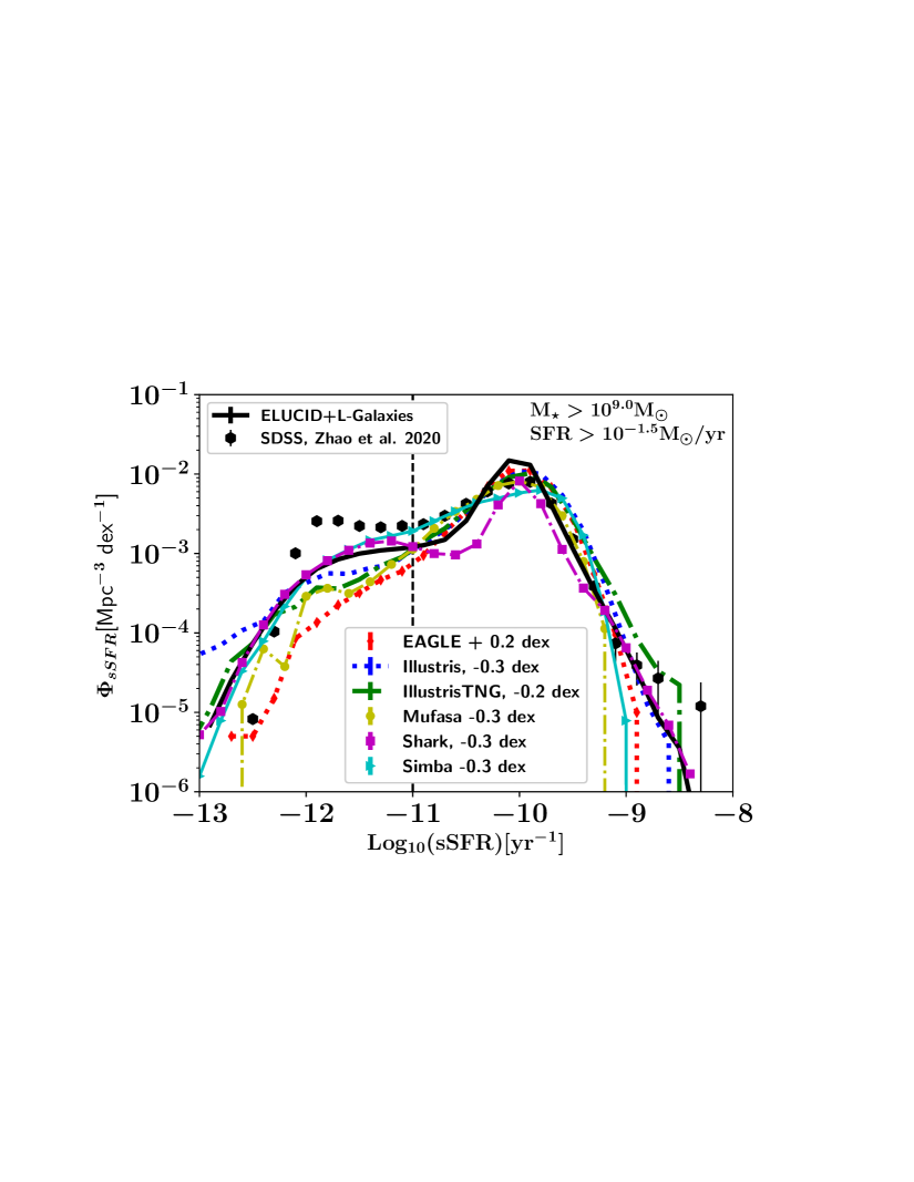
Figure 2: The sSFR in cosmological simulations: Illustris (blue dotted line, Genel et al., 2014), EAGLE (red diamond line, Schaye et al., 2015), Mufasa (yellow line with circles, Davé et al., 2017) , IllustrisTNG (green dashed-dotted line, Pillepich et al., 2018), Shark (magenta line with squares, Lagos et al., 2018), Simba (cyan line with triangles, Davé et al., 2019) and ELUCID+L-Galaxies (black solid line, Luo et al., 2016). Black hexagons represent the observed (Eddington bias corrected) sSFRF from Zhao et al. (2020). We see that the bi-modality found in observations is not reproduced for a range of cosmological models (Illustris, Mufasa, EAGLE, IllustrisTNG), with the ELUCID+L-Galaxies (described by the black solid line), Shark (magenta line with squares), Simba (cyan line with triangles) performing better qualitatively, since a bi-modality of sSFRs is emerging. However, even the latter have quantitatively lower number density peaks for quenched objects.

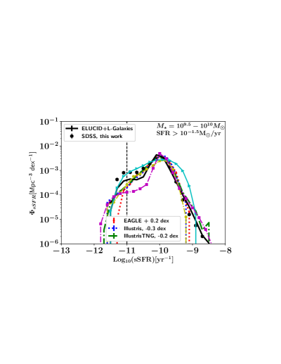
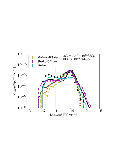
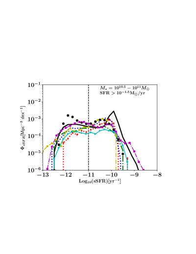
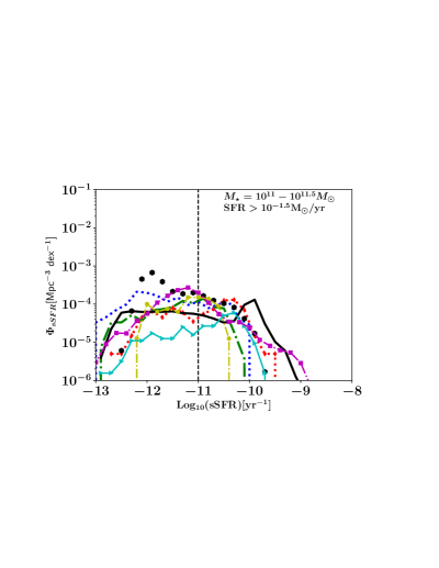
Figure 3: The sSFR at the mass scales/mass intervals of $10^{9.5}-10^{10.0}\,{\rm M_{\odot}}$ (top left panel), $10^{10.0}-10^{10.5}\,{\rm M_{\odot}}$ (top right panel), $10^{10.5}-10^{11.0}\,{\rm M_{\odot}}$ (bottom left panel) and $10^{11.0}-10^{11.5}\,{\rm M_{\odot}}$ (bottom right panel) for ${\rm SFRs>10^{-1.5}}$ ${\rm M_{\odot}/{\rm yr}}$ galaxies in cosmological simulations: Illustris (blue dotted line Genel et al., 2014), EAGLE (red line with diamonds Schaye et al., 2015), Mufasa (yellow line with circles Davé et al., 2017) , IllustrisTNG (green dashed-dotted line Pillepich et al., 2018), Simba (green line with triangles Davé et al., 2019), Shark (magenta line with squares, Lagos et al., 2018) and ELUCID+L-Galaxies (black solid line Luo et al., 2016). Black hexagons represent the Eddington bias corrected sSFRF from SDSS at different mass bins present at Fig. 1.

3.2 The Simulated versus the Observed sSFRF

We note that the comparisons we perform at this work are strictly done within the same limits for both observations and simulations (${\rm M_{\star}}>10^{9}$ ${\rm M_{\odot}}$ in terms of stellar mass and SFR $>10^{-1.5}$ ${\rm M_{\odot}/{\rm yr}}$). We also stress that the simulations discussed typically produce SFRFs (Davé et al., 2017; Katsianis et al., 2017b; Zhao et al., 2020) and GSMFs (by construction) in excellent agreement with observations and are supposed to not be affected by resolution effects within the above SFR and stellar mass limits.

Before comparing the different simulations with the observations present at Fig. 1 we investigate in Fig. 2 if models produce the bi-modal sSFRF described in Zhao et al. (2020) (black hexagons). Illustris is represented by the blue dotted line, EAGLE by the red line with diamonds, Mufasa is described by the yellow line with circles, IllustrisTNG by the green dashed-dotted line, Shark by the magenta line with squares, Simba by the green line with triangles and ELUCID+L-Galaxies by the dark solid line. In order to be able to perform the comparison qualitatively (the shape of the sSFRF) and be able to visually follow the lines of the plot we shift the originals lines in the x-axis by -0.3 dex, +0.2 dex, -0.3 dex, -0.3 dex, -0.3 dex, -0.3 dex and +0.0 dex, respectively. We note that any re-scaling is within the systematic uncertainties of different SFR indicators at low redshifts (Katsianis et al., 2016; Davies et al., 2016; Lower et al., 2020) and it is a common practice used in order to facilitate qualitative comparisons between different data-sets and simulations (McAlpine et al., 2017; Katsianis et al., 2019; Donnari et al., 2019). For example, EAGLE SFRs are reported to be 0.2 dex lower than observations (Katsianis et al., 2017b; McAlpine et al., 2017). Following, McAlpine et al. (2017) and Katsianis et al. (2019) we shift the simulated sSFRFs by +0.2 dex to focus on the shape of the distribution and facilitate a qualitative comparison with SDSS and the other cosmological simulations considered. On the other hand, Mufasa (Davé et al., 2017) has larger SFRs with respect to the H$\alpha$ observations of Gunawardhana et al. (2013) by 0.3 dex, so we shift the sSFRFs in Mufasa by this value (-0.3 dex). We perform a quantitative comparison without any re-scalings in Fig. 4.

Starting from Fig. 3 and the qualitative comparison we see that Illustris, EAGLE, Mufasa and IllustrisTNG resemble a uni-modal double-exponential Gausian (Ilbert et al., 2015; Katsianis et al., 2019) and while they are quite successful at reproducing the star-forming population and the related peak, they are unable to reproduce the secondary peak of quenched objects. The ELUCID+L-Galaxies model (described by the black solid line), Shark (magenta line with squares) and the Simba simulation (cyan line with triangles) perform better qualitatively with respect to the observations since a modest presence of a passive population emerges. However, even the latter have quantitatively lower number density of quenched objects compared to the SDSS observations.

In Fig. 3 we present the sSFRF at different stellar mass intervals of ${\rm M_{\star}}=10^{9.5}-10^{10.0}\,{\rm M_{\odot}}$ (top left panel), ${\rm M_{\star}}=10^{10.0}-10^{10.5}\,{\rm M_{\odot}}$ (top right panel), ${\rm M_{\star}}=10^{10.5}-10^{11.0}\,{\rm M_{\odot}}$ (bottom left panel) and ${\rm M_{\star}}=10^{11.0}-10^{11.5}\,{\rm M_{\odot}}$ (bottom right panel) of the cosmological simulations compared to our observational constraints. We see that Illustris (shifted by -0.3 dex), EAGLE (+0.2 dex), IllustrisTNG (-0.2 dex) and Mufasa (-0.3 dex) are in excellent qualitative agreement with each other at the ${\rm M_{\star}}=10^{9.0}-10^{9.5}\,{\rm M_{\odot}}$, ${\rm M_{\star}}=10^{9.5}-10^{10}\,{\rm M_{\odot}}$ and ${\rm M_{\star}}=10^{10}-10^{10.5}\,{\rm M_{\odot}}$ stellar mass bins. The above models reproduce successfully the star-forming peak of our SDSS observations. However, besides the differences between the different collaborations in quenching methods all the above models are unable to produce an adequate passive population within the strict limits we adopt and are unable to generate its associated peak. On the other hand, Simba (cyan line with triangles, original shifted by +0 dex), Shark (Magenta line with squares, -0.3 dex) and L-Galaxies (black solid line, + 0 dex) are able to reproduce bi-modal distributions at most stellar mass bins.

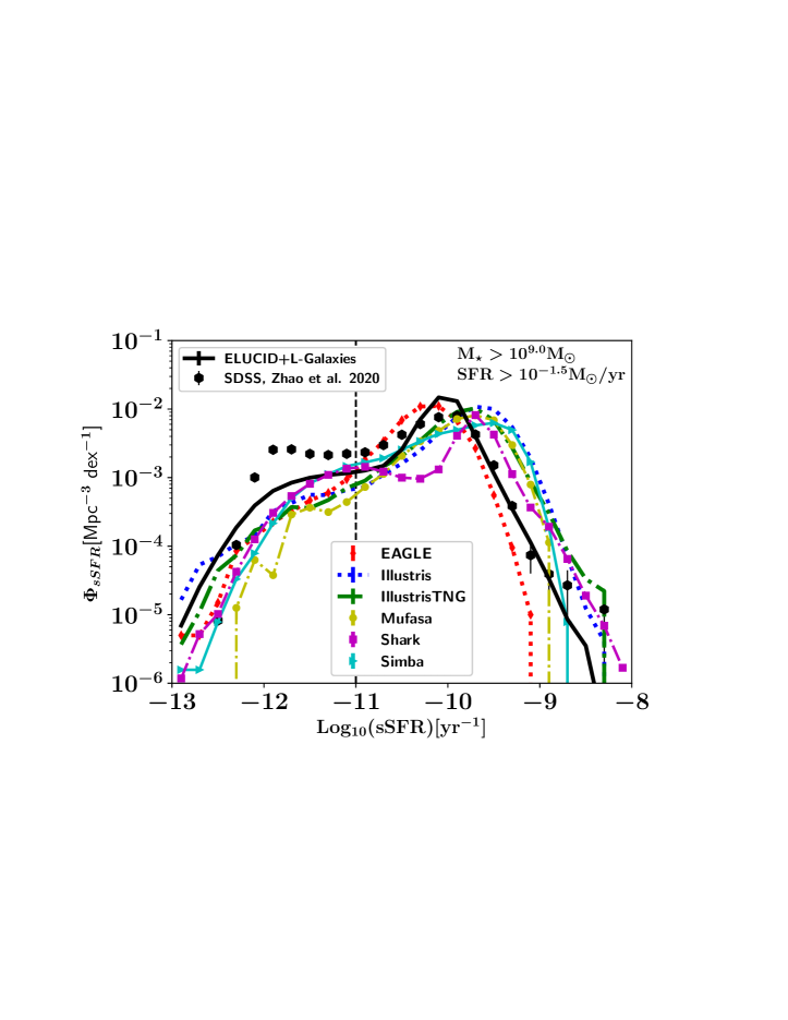
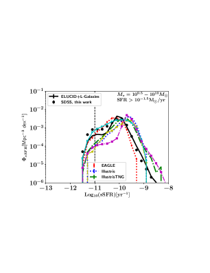
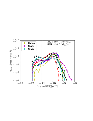
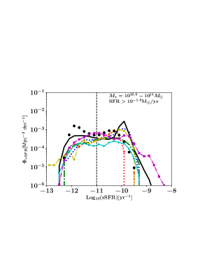
Figure 4: Same as Fig. 2 and Fig. 3 but no re-scaling was employed for the models.

Katsianis et al. (2019) performed comparisons between the sSFRFs of Ilbert et al. (2015) and EAGLE. As discussed in section 2 the study of Ilbert et al included star-forming objects only and excluded quenched galaxies by using a color-color selection. An agreement was demonstrated between simulations and observations without the need to exclude any “passive” objects from the simulation. Since there was not any necessity to apply a separation in order to achieve this agreement, it was implied that EAGLE does not produce many quenched galaxies within the sSFR $=$ $10^{-11}$ to $10^{-13}$ ${\rm yr^{-1}}$ range. The scarcity of passive objects within these regimes for the reference simulation of EAGLE has been noted in other studies as well (Katsianis et al., 2020; Trčka et al., 2020; Baes et al., 2020). Furlong et al. (2015) and Trayford et al. (2017) pointed out that a large number of the simulated galaxies in EAGLE (especially at the low-mass end) are influenced by numerical effects and poor particle sampling. This effect is responsible for low star formation rates for these un-resolved objects which appear quiescent with SFRs = 0. Their presence increases the passive fraction. However, this limitation is not enough to raise (as an artefact) an adequate passive population and a bi-modality for the simulated sSFRF, similar to the one found in SDSS (Fig. 1 and Fig. 3). We find that 20 $\%$ of simulated galaxies at ${\rm M_{\star}}=10^{9.5}-10^{10}\,{\rm M_{\odot}}$, 18 $\%$ at the ${\rm M_{\star}}=10^{10}-10^{10.5}\,{\rm M_{\odot}}$, 17 $\%$ at the ${\rm M_{\star}}=10^{10.5}-10^{11}\,{\rm M_{\odot}}$ and 13 $\%$ at ${\rm M_{\star}}=10^{11}-10^{11.5}\,{\rm M_{\odot}}$ have SFRs equal to 0. It is a common practice (Davé et al., 2019) for these objects, since they are considered a by-product of limitations of resolution, to be granted artificially higher sSFRs and to be added at the last bin considered by the analysis (in our case sSFR $=$ $10^{-12.9}{\rm yr^{-1}}$). We stress that this is not enough to display a similar sSFR distribution as seen in SDSS, since the other sSFR bins representing passive objects (e.g. sSFR = $10^{-11}-10^{-12.7}{\rm yr^{-1}}$) would remain unaffected by the above procedure (i.e. we would produce only an artificial peak and not the total secondary gaussian distribution). Following another approach we could grant an artificial gaussian distribution of SFRs to the objects with SFR = 0, below the SFR resolution limit of the simulation (e.g. SFRs within $10^{-4}-10^{-5}$ ${\rm M_{\odot}/{\rm yr}}$, Fig. 8 Donnari et al., 2019). However, these objects with artificially granted SFRs would be excluded from our analysis which adopts a strict limit (${\rm SFRs>10^{-1.5}}$ ${\rm M_{\odot}/{\rm yr}}$) both in SDSS and simulations (i.e. un-resolved objects with SFRs = 0 would be granted SFR values below the resolution limit and thus would not affect the comparisons performed in Fig. 2 and Fig. 3.). We note that EAGLE represents the model, within our study, with the least active objects (distribution appears shifted towards lower sSFRs with respect the observations and the rest simulations). The peak representing the main sequence appears quantitatively 0.2 dex lower (at sSFR = $10^{-10.2}{\rm yr^{-1}}$) than the one found in SDSS observations (at sSFR = $10^{-10.0}{\rm yr^{-1}}$) and 0.5 dex lower than the one found in Illustris (Fig. 4), showing that the thermal feedback scheme employed in EAGLE is very effective. We note that the AGN feedback scheme, which does not separate between radio mode and quasar mode (subsection 3), does not yield results qualitatively different from other models like Illustris-TNG (Fig. 2 and Fig. 3) that uses a more sophisticated prescription.

Similarly to Katsianis et al. (2019), Davé et al. (2017) demonstrated that Mufasa is successful at reproducing the observations of Ilbert et al. (2015) and suggested that this implies that the model is able to quench galaxies successfully. As suggested in the previous paragraph, we believe that this comparison does not provide evidence of a successful quenching scheme since these observations do not include passive objects by construction. The comparison is strictly performed for galaxies of sSFR $=$ $10^{-11}$-$10^{-9}$ ${\rm yr^{-1}}$ (i.e. star-forming objects). The authors pointed that there is still a notable number of star-forming galaxies even at the highest stellar masses in Mufasa. Our analysis agrees quite well with this statement and supports the idea of having numerous star-forming galaxies even at the highest mass regime, with quenched galaxies however being more dominant (bottom panels of Fig. 3). We note that the quenching mechanism adopted in Mufasa combined with limitations in resolution are responsible for totally halting star formation (SFR = 0) for 40 $\%$ of the simulated objects with $M_{\star}>10^{9}\,{\rm M_{\odot}}$. These “dead” objects if allowed to retain some level of star formation (advances in resolution and especially modeling are required for this step) can potentially generate a secondary gaussian distribution similar to SDSS. As discussed in the previous subsection, cosmological models that attempt to follow both dark matter and gas suffer from limitations in resolution and box-size. We have to note that Mufasa is the simulation, within our work, with the lowest resolution and smallest volume. The numbers of objects at the high- and low- mass ends can be affected by these shortcomings and this in return can impact the retrieved sSFRF. If high mass and passive objects are under-represented in a simulation then the sSFR distribution describing the quenched population will unavoidably be incomplete. Besides these limitations and the fact that Mufasa does not employ a full treatment for the AGN feedback (i.e. uses just a scheme to resemble a radio-mode back reaction via heating) it produces qualitatively (Fig. 2 and Fig. 3) and quantitatively (Fig. 4) sSFRFs in perfect agreement with Illustris which has 16 times higher mass resolution and 3 times larger volume. This comparison is a good example of how two completely different cosmological simulations with different feedback schemes, resolutions and volumes produce similar results due to a thoughtful tuning of their subgrid Physics for their adopted resolutions.

Contrary to Mufasa (yellow line with circles), its successor Simba (cyan line with triangles) produces a different distribution qualitatively and is able to produce a clear bi-modality for the ${\rm M_{\star}}=10^{10}-10^{10.5}\,{\rm M_{\odot}}$ and ${\rm M_{\star}}=10^{10.5}-10^{11}\,{\rm M_{\odot}}$ stellar mass bins. We consider this a success, possibly related to the updated model and the inclusion of a quenching feedback prescription via AGN. In addition to the kinetic AGN back reaction, Simba also includes an X-ray feedback input. The importance of the X-ray heating has been explored in zoom simulations by Choi et al. (2012), showing that it can potentially drive the quenching of massive galaxies. Simba is the first cosmological-volume simulation to include such a mechanism and according to Davé et al. (2019), this heating besides the fact that it has a minimum effect on the GSMF, it provides an important factor to fully quench galaxies. Without the X-ray feedback component and only the kinetic back reaction from jets, Simba would not generate an adequate number of objects below sSFR $=$ $10^{-11}$ ${\rm yr^{-1}}$, and instead would generate mostly galaxies between sSFR $=$ $10^{-10}$ ${\rm yr^{-1}}$ and sSFR $=$ $10^{-9}$ ${\rm yr^{-1}}$ (like Illustris, or EAGLE). So the X-ray feedback plays a major role in Simba in reproducing quenched galaxies. Davé et al. (2019) demonstrated that a bi-modal form emerges for the histograms of the simulated sSFRs and this is in agreement with the observed distributions obtained from the GALEX-SDSS-WISE Legacy CatalogS (GSWLC, Salim et al., 2016). The difference between Mufasa and Simba is that due to the updated AGN feedback mechanism, the Simba simulation has less star-forming objects, especially at higher masses. The affected galaxies have “moved” towards lower sSFRs and a bi-modality has emerged. However, this approach decreased significantly the star-forming population and its associated peak has a lower number density than the one found in our observations. We stress that in Simba 40 $\%$ of galaxies at ${\rm M_{\star}}=10^{10.5}-10^{11}\,{\rm M_{\odot}}$ and 60 $\%$ at ${\rm M_{\star}}=10^{11}-10^{11.5}\,{\rm M_{\odot}}$ have SFRs equal to 0. The above demonstrates the high efficiency of the kinetic and X-ray feedback prescriptions adopted in Simba for high mass objects. We also see the importance of the quenching mechanisms in totally pausing SF in simulated galaxies and generating “dead” objects with SFR = 0. A more moderate quenching mechanism, would allow more objects to retain a low level of non-zero SFR, a larger normalization for the sSFRF and better quantitative agreement with observations.

Furthermore, we demonstrate that IllustrisTNG sSFRFs (dashed green lines of Fig. 3) are not bi-modal at any mass bins considered. Illustris performs similarly to TNG except in the last stellar mass bin (bottom panel of Fig 3). TNG, while keeping the good resolution and statistics of Illustris, includes a range of improvements with respect to the original illustris which made the updated model much more successful in terms of replicating key observables. One of those is the color bi-modality of SDSS (Nelson et al., 2018). As we suggested in the introduction, color and sSFRs are directly related so it would be expected that this success would be imprinted in the TNG sSFRFs as well. However, we obtain a uni-modal distribution for the simulation . We note that the comparison between SDSS and TNG performed at Fig. 3 is strictly done well above the SFR resolution limits of the simulation (${\rm SFRs\sim 10^{-3}}$ ${\rm M_{\odot}/{\rm yr}}$) and thus even by granting artificial SFR greater than 0 (but lower than the resolution limit) to the numerous “dead” un-resolved objects, still these SFRs would be well below the ${\rm SFRs\sim 10^{-1.5}}$ ${\rm M_{\odot}/{\rm yr}}$ threshold we adopted in our study and would result to ${\rm sSFRs}<10^{-13}$ ${\rm yr^{-1}}$ (e.g. Donnari et al., 2019, granted these objects SFRs within $10^{-4}-10^{-5}$ ${\rm M_{\odot}/{\rm yr}}$). This points to the direction that the discrepancy seen between the SDSS observations and TNG has its roots in modeling and not limits in resolution.

Finally, we show that the ELUCID+LGalaxies (black solid line of Fig. 3) and Shark (magenta line with squares of Fig. 3) models show promising bi-modal sSFRFs. The success of L-Galaxies is due to the fact that it allows passive objects to retain a low level of star-forming activity and generate a secondary distribution of passive objects and the associated peak. We note that the total number of galaxies with SFR = 0 is only 2 $\%$, thus numerous objects with low SFRs emerge instead of “dead” galaxies and a bi-modality arises. However, ELUCID+LGalaxies has typically sharper peaks found than observations, while the Shark passive population in the ${\rm M_{\star}}=10^{10}-10^{10.5}\,{\rm M_{\odot}}$ and ${\rm M_{\star}}=10^{10.5}-10^{11.0}\,{\rm M_{\odot}}$ mass bins is not in quantitative agreement with the observed sSFRs, besides the non uni-modal forms . We note that both Shark and L-galaxies allow gas-poor galaxies to be less efficient in SF compared to gas-rich galaxies at a fixed gas surface density, either by using molecular gas-based SF prescriptions or a gas surface density threshold (Lagos et al., 2011) and this can enhance the sSFR bi-modality.

For both SAMs and cosmological simulations a thoughtful tuning of the parameters of the models that describe key processes of galaxy formation is required using observational constraints (Lacey et al., 2016), like the GSMF or the CSFRD. Because of their little computational expense, the tuning of parameters in SAMs can be easily done via MCMC, emulators or genetic algorithms (e.g. Bower et al., 2012; Henriques et al., 2013; Ruiz et al., 2015), while this task is much more demanding in hydrodynamical simulations. This may be playing an important role in why SAMs perform qualitatively better than most hydrodynamical simulations explored here. However, the tuning done for any case scenario alone cannot guarantee a success for a model since any “mistakes” in the recipes that describe gas, star formation and feedback can be compensated through tuning and various observations can be “successfully” reproduced. We suggest that the sSFRF can provide a useful test/constraint since it encloses information about galaxy quenching and the relation between SFR and stellar mass.

4 Conclusions

In this work we investigated the Specific Star Formation Rate Function (sSFRF) across different mass scales (${\rm M_{\star}}=10^{9.0}-10^{9.5}\,{\rm M_{\odot}}$, ${\rm M_{\star}}=10^{10}-10^{10.5}\,{\rm M_{\odot}}$, ${\rm M_{\star}}=10^{10.5}-10^{11}\,{\rm M_{\odot}}$ and ${\rm M_{\star}}=10^{11}-10^{11.5}\,{\rm M_{\odot}}$) in the Sloan Digital Sky Survey Data Release 7 (SDSS) for objects within the survey’s SFRs and Stellar mass confidence limits (${\rm M_{\star}}>10^{9}$ ${\rm M_{\odot}}$, ${\rm SFR}$ $>$ $10^{-1.5}$ ${\rm M_{\odot}/{\rm yr}}$, Weigel et al., 2016; Zhao et al., 2020). The above enable us to study qualitatively and quantitatively quenching, the distribution of passive/star-forming galaxies and compare the results with the predictions from state-of-the-art cosmological simulations and semi-analytic models (SAMs). The latter have been found to reproduce the observed SFRF and GSMF at $z\sim 0$, while they typically do not suffer from limitations of resolution within the ranges we adopt (Katsianis et al., 2017b; Zhao et al., 2020). Our main conclusions are summarized as follows:

• The sSFRF (star-forming + quiescent) at different mass scales is bi-modal (section 2). This form is in agreement with the findings of other studies which employed other data-sets at various redshifts (Santini et al., 2009; Tzanavaris et al., 2010; Lenkić et al., 2016; Davé et al., 2019) and previous studies of the SDSS (Wetzel et al., 2012). Galaxies, within our ${\rm M_{\star}}$ and SFR limits, become more passive with increasing stellar mass but the transition across different mass scales is rather smooth. The low mass end (${\rm M_{\star}}=10^{9.5}-10^{10}\,{\rm M_{\odot}}$) is mostly dominated by star forming galaxies with our results from SDSS being in excellent agreement with the main-sequence (star-forming galaxies only) study of Ilbert et al. (2015). However, moving to the intermediate mass bins (${\rm M_{\star}}=10^{10}-10^{10.5}\,{\rm M_{\odot}}$ and ${\rm M_{\star}}=10^{10.5}-10^{11}\,{\rm M_{\odot}}$) we see already an arising passive population, which gives a bi-modal form to the sSFRF. At higher masses (${\rm M_{\star}}=10^{11}-10^{11.5}\,{\rm M_{\odot}}$) we find a notable star forming population, in agreement with the main-sequence study of Ilbert et al. (2015) and the predictions from cosmological simulations (Davé et al., 2017).

• The Simba, L-galaxies and Shark models generate bi-modal sSFRFs and thus are qualitatively in agreement with our findings for SDSS (section 3). We stress that none of these models was tuned to reproduce this behavior. The above is achieved since all models are able to create both star-forming galaxies (sSFR $>$ $10^{-11}{\rm yr^{-1}}$) and an arising with mass passive population (sSFR $<$ $10^{-11}{\rm yr^{-1}}$), within the same ${\rm M_{\star}}$ and SFR limits as those adopted in observations. We note however, that besides that Simba sSFRF is bi-modal (Davé et al., 2019) it does not match quantitatively SDSS which has typically higher number density values. Simba achieved its sSFR distributions by moving numerous star-forming galaxies towards the passive population via its efficient AGN feedback and as a result underpredicts the peak of the active objects with respect observations. On the other hand, the Shark and L-galaxies semi-analytic models appear to retain the high numbers of their star-forming galaxies and allowed passive objects to maintain low levels of SFR. The presence of the latter generate an adequate quenched population with ${\rm sSFR}\sim 10^{-12}-10^{-11}\,{\rm yr^{-1}}$. A tuning of both effects found in Simba (decreasing the star forming population to generate more quenched objects) and L-Galaxies (allowing “dead” galaxies with SFR = 0 to retain a higher level of SF activity) could bring in better agreement the observed and simulated sSFRFs.

• Illustris, EAGLE, Mufasa and IllustrisTNG successfully produce the sSFRF of star forming galaxies and are in excellent agreement with the sSFRF from SDSS at sSFR $>$ $10^{-11}{\rm yr^{-1}}$ at all mass regimes. However, the same models are unable to generate an adequate population of passive galaxies with sSFRs between $10^{-11}{\rm yr^{-1}}$ and $10^{-13}{\rm yr^{-1}}$ in order to establish a bi-modality at any mass range considered in this work. Instead the above simulations demonstrate a uni-modal sSFRF in contrast with Simba, L-Galaxies and our results from SDSS. We note that the Illustris, Mufasa and TNG cosmological simulations adopt different feedback schemes, resolutions and volumes but still produce similar results for the sSFRF. Different models can achieve similar star formation histories (SFHs) We propose that the feedback and star formation prescriptions that are used in state-of-the-art cosmological simulations have to be reconsidered, involve recipes that allow “quenched galaxies” to retain a small level of SF activity (sSFR $=$ ${\rm 10^{-11}{\rm yr^{-1}}}$-${\rm 10^{-12}{\rm yr^{-1}}}$) and generate an adequate passive population/bi-modality even at intermediate masses (${\rm M_{\star}}=10^{10}-10^{10.5}\,{\rm M_{\odot}}$).

Data Availability Statement

No new data were generated or analyzed in support of this research.

References

- Abazajian et al. (2009) Abazajian K. N., et al., 2009, ApJS, 182, 543
- Anglés-Alcázar et al. (2017a) Anglés-Alcázar D., Faucher-Giguère C.-A., Kereš D., Hopkins P. F., Quataert E., Murray N., 2017a, MNRAS, 470, 4698
- Anglés-Alcázar et al. (2017b) Anglés-Alcázar D., Faucher-Giguère C.-A., Quataert E., Hopkins P. F., Feldmann R., Torrey P., Wetzel A., Kereš D., 2017b, MNRAS, 472, L109
- Baes et al. (2020) Baes M., et al., 2020, MNRAS, 494, 2912
- Baldry et al. (2008) Baldry I. K., Glazebrook K., Driver S. P., 2008, MNRAS, 388, 945
- Belfiore et al. (2018) Belfiore F., et al., 2018, MNRAS, 477, 3014
- Bell (2003) Bell E. F., 2003, ApJ, 586, 794
- Benson & Bower (2011) Benson A. J., Bower R., 2011, MNRAS, 410, 2653
- Blanc et al. (2019) Blanc G. A., Lu Y., Benson A., Katsianis A., Barraza M., 2019, ApJ, 877, 6
- Bower et al. (2012) Bower R. G., Benson A. J., Crain R. A., 2012, MNRAS, 422, 2816
- Bower et al. (2017) Bower R. G., Schaye J., Frenk C. S., Theuns T., Schaller M., Crain R. A., McAlpine S., 2017, MNRAS, 465, 32
- Bravo et al. (2020) Bravo M., Lagos C. d. P., Robotham A. S. G., Bellstedt S., Obreschkow D., 2020, arXiv e-prints, p. arXiv:2003.11258
- Brinchmann et al. (2004) Brinchmann J., Charlot S., White S. D. M., Tremonti C., Kauffmann G., Heckman T., Brinkmann J., 2004, MNRAS, 351, 1151
- Cantiello & Blakeslee (2007) Cantiello M., Blakeslee J. P., 2007, ApJ, 669, 982
- Caplar & Tacchella (2019) Caplar N., Tacchella S., 2019, MNRAS, 487, 3845
- Carter et al. (2009) Carter D., et al., 2009, MNRAS, 397, 695
- Cassata et al. (2010) Cassata P., et al., 2010, ApJ, 714, L79
- Chabrier (2003) Chabrier G., 2003, PASP, 115, 763
- Chen et al. (2019) Chen Y., Mo H. J., Li C., Wang H., Yang X., Zhou S., Zhang Y., 2019, ApJ, 872, 180
- Choi et al. (2012) Choi E., Ostriker J. P., Naab T., Johansson P. H., 2012, ApJ, 754, 125
- Concas et al. (2019) Concas A., Popesso P., Brusa M., Mainieri V., Thomas D., 2019, A&A, 622, A188
- Cowie & Barger (2008) Cowie L. L., Barger A. J., 2008, ApJ, 686, 72
- Crain et al. (2015) Crain R. A., et al., 2015, MNRAS, 450, 1937
- Croton (2013) Croton D. J., 2013, PASA, 30, e052
- Croton et al. (2006a) Croton D. J., et al., 2006a, MNRAS, 365, 11
- Croton et al. (2006b) Croton D. J., et al., 2006b, MNRAS, 367, 864
- Croton et al. (2016) Croton D. J., et al., 2016, ApJS, 222, 22
- Dai et al. (2018) Dai Y. S., Wilkes B. J., Bergeron J., Kuraszkiewicz J., Omont A., Atanas A., Teplitz H. I., 2018, MNRAS, 478, 4238
- Dalla Vecchia & Schaye (2012) Dalla Vecchia C., Schaye J., 2012, MNRAS, 426, 140
- Darvish et al. (2018) Darvish B., Martin C., Gonçalves T. S., Mobasher B., Scoville N. Z., Sobral D., 2018, ApJ, 853, 155
- Davé et al. (2011) Davé R., Oppenheimer B. D., Finlator K., 2011, MNRAS, 415, 11
- Davé et al. (2017) Davé R., Rafieferantsoa M. H., Thompson R. J., Hopkins P. F., 2017, MNRAS,
- Davé et al. (2019) Davé R., Anglés-Alcázar D., Narayanan D., Li Q., Rafieferantsoa M. H., Appleby S., 2019, MNRAS, 486, 2827
- Davies et al. (2016) Davies L. J. M., et al., 2016, MNRAS, 461, 458
- Davies et al. (2019a) Davies L. J. M., et al., 2019a, MNRAS, 483, 1881
- Davies et al. (2019b) Davies L. J. M., et al., 2019b, MNRAS, 483, 5444
- Di Matteo et al. (2008) Di Matteo T., Colberg J., Springel V., Hernquist L., Sijacki D., 2008, ApJ, 676, 33
- Donnari et al. (2019) Donnari M., et al., 2019, MNRAS, 485, 4817
- Dubois et al. (2014) Dubois Y., et al., 2014, MNRAS, 444, 1453
- Eddington (1913) Eddington A. S., 1913, MNRAS, 73, 359
- Elahi et al. (2018) Elahi P. J., Welker C., Power C., Lagos C. d. P., Robotham A. S. G., Cañas R., Poulton R., 2018, MNRAS, 475, 5338
- Elahi et al. (2019) Elahi P. J., Cañas R., Poulton R. J. J., Tobar R. J., Willis J. S., Lagos C. d. P., Power C., Robotham A. S. G., 2019, PASA, 36, e021
- Fabian (2012) Fabian A. C., 2012, ARA&A, 50, 455
- Fang et al. (2018) Fang J. J., et al., 2018, ApJ, 858, 100
- Feldmann (2017) Feldmann R., 2017, MNRAS, 470, L59
- Firmani & Avila-Reese (2010) Firmani C., Avila-Reese V., 2010, ApJ, 723, 755
- Fu et al. (2010) Fu J., Guo Q., Kauffmann G., Krumholz M. R., 2010, MNRAS, 409, 515
- Fu et al. (2013) Fu J., et al., 2013, MNRAS, 434, 1531
- Furlong et al. (2015) Furlong M., et al., 2015, MNRAS, 450, 4486
- Gabor & Davé (2012) Gabor J. M., Davé R., 2012, MNRAS, 427, 1816
- García et al. (2017) García L. A., Tescari E., Ryan-Weber E. V., Wyithe J. S. B., 2017, MNRAS, 470, 2494
- Genel et al. (2014) Genel S., et al., 2014, MNRAS, 445, 175
- Gunawardhana et al. (2013) Gunawardhana M. L. P., et al., 2013, MNRAS, 433, 2764
- Hahn et al. (2019) Hahn C., et al., 2019, ApJ, 872, 160
- Hall et al. (2018) Hall K. R., Crichton D., Marriage T., Zakamska N. L., Mandelbaum R., 2018, MNRAS, 480, 149
- Henriques et al. (2013) Henriques B. M. B., White S. D. M., Thomas P. A., Angulo R. E., Guo Q., Lemson G., Springel V., 2013, MNRAS, 431, 3373
- Henriques et al. (2015) Henriques B. M. B., White S. D. M., Thomas P. A., Angulo R., Guo Q., Lemson G., Springel V., Overzier R., 2015, MNRAS, 451, 2663
- Hirschmann et al. (2012) Hirschmann M., Naab T., Somerville R. S., Burkert A., Oser L., 2012, MNRAS, 419, 3200
- Hopkins (2015) Hopkins P. F., 2015, MNRAS, 450, 53
- Ilbert et al. (2013) Ilbert O., McCracken H. J., Le Fèvre O., et al., 2013, A&A, 556, A55
- Ilbert et al. (2015) Ilbert O., et al., 2015, A&A, 579, A2
- Katsianis et al. (2015) Katsianis A., Tescari E., Wyithe J. S. B., 2015, MNRAS, 448, 3001
- Katsianis et al. (2016) Katsianis A., Tescari E., Wyithe J. S. B., 2016, PASA, 33, e029
- Katsianis et al. (2017a) Katsianis A., Tescari E., Blanc G., Sargent M., 2017a, MNRAS, 464, 4977
- Katsianis et al. (2017b) Katsianis A., et al., 2017b, MNRAS, 472, 919
- Katsianis et al. (2019) Katsianis A., et al., 2019, The Astrophysical Journal, 879, 11
- Katsianis et al. (2020) Katsianis A., et al., 2020, MNRAS, 492, 5592
- Kroupa (2001) Kroupa P., 2001, MNRAS, 322, 231
- Krumholz (2013) Krumholz M. R., 2013, MNRAS, 436, 2747
- Lacey et al. (2016) Lacey C. G., et al., 2016, MNRAS, 462, 3854
- Lagos et al. (2011) Lagos C. D. P., Lacey C. G., Baugh C. M., Bower R. G., Benson A. J., 2011, MNRAS, 416, 1566
- Lagos et al. (2013) Lagos C. d. P., Lacey C. G., Baugh C. M., 2013, MNRAS, 436, 1787
- Lagos et al. (2018) Lagos C. d. P., Tobar R. J., Robotham A. S. G., Obreschkow D., Mitchell P. D., Power C., Elahi P. J., 2018, MNRAS, 481, 3573
- Lenkić et al. (2016) Lenkić L., et al., 2016, MNRAS, 459, 2948
- Li & White (2009) Li C., White S. D. M., 2009, MNRAS, 398, 2177
- Li et al. (2007) Li Z., Han Z., Zhang F., 2007, A&A, 464, 853
- Lopez et al. (2020) Lopez S., et al., 2020, MNRAS, 491, 4442
- Lovell et al. (2020) Lovell C. C., Vijayan A. P., Thomas P. A., Wilkins S. M., Barnes D. J., Irodotou D., Roper W., 2020, arXiv e-prints, p. arXiv:2004.07283
- Lower et al. (2020) Lower S., Narayanan D., Leja J., Johnson B. D., Conroy C., Davé R., 2020, arXiv e-prints, p. arXiv:2006.03599
- Lu et al. (2020) Lu Y., Yang X., Liu C., Guo H., Xu H., Katsianis A., Wang Z., 2020, arXiv e-prints, p. arXiv:2008.09804
- Luo et al. (2016) Luo Y., Kang X., Kauffmann G., Fu J., 2016, MNRAS, 458, 366
- Madau & Dickinson (2014) Madau P., Dickinson M., 2014, ARA&A, 52, 415
- Matthee & Schaye (2019) Matthee J., Schaye J., 2019, MNRAS, 484, 915
- McAlpine et al. (2017) McAlpine S., Bower R. G., Harrison C. M., Crain R. A., Schaller M., Schaye J., Theuns T., 2017, MNRAS, 468, 3395
- Mitchell et al. (2018) Mitchell P. D., et al., 2018, MNRAS, 474, 492
- Muratov et al. (2015) Muratov A. L., Kereš D., Faucher-Giguère C.-A., Hopkins P. F., Quataert E., Murray N., 2015, MNRAS, 454, 2691
- Nelson et al. (2018) Nelson D., et al., 2018, MNRAS, 475, 624
- Okamoto et al. (2010) Okamoto T., Frenk C. S., Jenkins A., Theuns T., 2010, MNRAS, 406, 208
- Perna et al. (2017) Perna M., Lanzuisi G., Brusa M., Mignoli M., Cresci G., 2017, A&A, 603, A99
- Pillepich et al. (2018) Pillepich A., et al., 2018, MNRAS, 473, 4077
- Planck Collaboration et al. (2016) Planck Collaboration et al., 2016, A&A, 596, A106
- Puchwein & Springel (2013) Puchwein E., Springel V., 2013, MNRAS, 428, 2966
- Rosas-Guevara et al. (2015) Rosas-Guevara Y. M., et al., 2015, MNRAS, 454, 1038
- Rosas-Guevara et al. (2016) Rosas-Guevara Y., Bower R. G., Schaye J., McAlpine S., Dalla Vecchia C., Frenk C. S., Schaller M., Theuns T., 2016, MNRAS, 462, 190
- Ruiz et al. (2015) Ruiz A. N., et al., 2015, ApJ, 801, 139
- Salim et al. (2007) Salim S., Rich R. M., Charlot S., Brinchmann J., et al., 2007, ApJS, 173, 267
- Salim et al. (2016) Salim S., et al., 2016, ApJS, 227, 2
- Santini et al. (2009) Santini P., et al., 2009, A&A, 504, 751
- Schaye et al. (2015) Schaye J., et al., 2015, MNRAS, 446, 521
- Sijacki et al. (2007) Sijacki D., Springel V., Di Matteo T., Hernquist L., 2007, MNRAS, 380, 877
- Sijacki et al. (2008) Sijacki D., Pfrommer C., Springel V., Enßlin T. A., 2008, MNRAS, 387, 1403
- Springel (2005) Springel V., 2005, MNRAS, 364, 1105
- Springel (2010) Springel V., 2010, MNRAS, 401, 791
- Strateva et al. (2001) Strateva I., et al., 2001, AJ, 122, 1861
- Tamburri et al. (2014) Tamburri S., Saracco P., Longhetti M., Gargiulo A., Lonoce I., Ciocca F., 2014, A&A, 570, A102
- Tescari et al. (2014) Tescari E., Katsianis A., Wyithe J. S. B., Dolag K., Tornatore L., Barai P., Viel M., Borgani S., 2014, MNRAS, 438, 3490
- Thomas et al. (2019) Thomas R., et al., 2019, A&A, 630, A145
- Trayford et al. (2017) Trayford J. W., et al., 2017, MNRAS, 470, 771
- Trčka et al. (2020) Trčka A., et al., 2020, MNRAS, 494, 2823
- Twite et al. (2012) Twite J. W., Conselice C. J., Buitrago F., Noeske K., Weiner B. J., Acosta-Pulido J. A., Bauer A. E., 2012, MNRAS, 420, 1061
- Tzanavaris et al. (2010) Tzanavaris P., et al., 2010, ApJ, 716, 556
- Vogelsberger et al. (2013) Vogelsberger M., Genel S., Sijacki D., Torrey P., Springel V., Hernquist L., 2013, MNRAS, 436, 3031
- Vogelsberger et al. (2014) Vogelsberger M., et al., 2014, MNRAS, 444, 1518
- Volonteri et al. (2016) Volonteri M., Dubois Y., Pichon C., Devriendt J., 2016, MNRAS, 460, 2979
- Wang et al. (2014) Wang H., Mo H. J., Yang X., Jing Y. P., Lin W. P., 2014, ApJ, 794, 94
- Wang et al. (2016) Wang H., et al., 2016, ApJ, 831, 164
- Wang et al. (2018) Wang H., et al., 2018, ApJ, 852, 31
- Wei et al. (2018) Wei C., et al., 2018, ApJ, 853, 25
- Weigel et al. (2016) Weigel A. K., Schawinski K., Bruderer C., 2016, MNRAS, 459, 2150
- Weinberger et al. (2017) Weinberger R., et al., 2017, MNRAS, 465, 3291
- Wetzel et al. (2012) Wetzel A. R., Tinker J. L., Conroy C., 2012, MNRAS, 424, 232
- Yang et al. (2018) Yang X., et al., 2018, ApJ, 860, 30
- Zhao et al. (2020) Zhao P., Xu H., Katsianis A., Yang X., 2020, arXiv e-prints, p. arXiv:2006.08634
- van den Bosch et al. (2008) van den Bosch F. C., Aquino D., Yang X., Mo H. J., Pasquali A., McIntosh D. H., Weinmann S. M., Kang X., 2008, MNRAS, 387, 79