Flow-FL: Data-Driven Federated Learning
for Spatio-Temporal Predictions in Multi-Robot Systems

Abstract

In this paper, we show how the Federated Learning (FL) framework enables learning collectively from distributed data in connected robot teams. This framework typically works with clients collecting data locally, updating neural network weights of their model, and sending updates to a server for aggregation into a global model. We explore the design space of FL by comparing two variants of this concept. The first variant follows the traditional FL approach in which a server aggregates the local models. In the second variant, that we call Flow-FL, the aggregation process is serverless thanks to the use of a gossip-based shared data structure. In both variants, we use a data-driven mechanism to synchronize the learning process in which robots contribute model updates when they collect sufficient data. We validate our approach with an agent trajectory forecasting problem in a multi-agent setting. Using a centralized implementation as a baseline, we study the effects of staggered online data collection, and variations in dataflow, number of participating robots, and time delays introduced by the decentralization of the framework in a multi-robot setting.

I INTRODUCTION

Robot swarms promise capabilities beyond the reach of single-robot solutions by distributing intelligence, sensing and actuation at a large scale [1]. This opportunity often comes with the challenge of dealing with large amounts of data which are physically distributed across robots. Replicating, broadcasting, and learning large-scale data has prohibitive communication and memory costs.

Federated Learning (FL) [2] is a recent approach to distributed machine learning that takes advantage of distributed data sets by partitioning learning on several machines. Data sets are partitioned either for excessive size, or because of the necessity to ensure data privacy among different data sources. In FL, individual clients collect data and calculate a local model update that is subsequently aggregated into a shared model by a dedicated server.

In a multi-robot setting, FL is a natural approach because it takes advantage of the inherently local fashion in which robots collect and process data. However, a practical approach to realizing FL in this setting is currently missing [3].

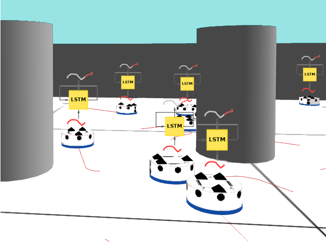
Figure 1: Federated Learning for collective trajectory forecasting in a multi-robot setting.

In this paper, we conduct a study of the design space of FL solutions in a multi-robot setting. We compare two variants. In the first, inspired by the original FL idea, a server aggregates the model updates calculated by the robots. In the second, the server is replaced by a shared data structure.

In both cases, a central problem is how to synchronize the learning process. Data is typically collected at diverse rates across a team of robots. This affects the frequency at which robots contribute to the update of the shared model. To cope with this issue, we propose a data-driven approach in which only the robots that have collected sufficient data calculate a model update and share it with the rest of the system. Being dependent on the data flow, we named our fully distributed approach Flow-FL.

We envision our approach to be effective in scenarios in which data varies across both time and space. To validate this insight, we consider multi-robot navigation in densely occupied environments. In these environments, the intent of other moving entities may be unknown, and the density and motion patterns might vary over time. Recent work focuses on the creation of machine learning approaches to model motion trajectories that enable predictive navigation [4]. In our approach, the robots build a shared trajectory model using locally collected data.

The main contributions of our paper are:

• We conduct an exploration of the design space of FL in robotics settings, comparing a variant in which models are aggregated on the server with a variant in which data is aggregated in a serverless, shared data structure;

• We apply the proposed approaches to a trajectory prediction problem and make our open-source federated dataset available for the research community;

• Using a centralized implementation as a baseline, we study the effects of staggered online data collection, variations in dataflow, number of participating robots, and time delays introduced by the decentralization of the framework in a multi-robot setting.

The paper is organized as follows. We discuss related work in Section II and formalize the problem in Section III. The design of our framework is presented in Section IV. We report the results of our performance evaluation in Section V, and conclude the paper in Section VI.

II RELATED WORK

Early attempts at distributed machine learning were based on centrally stored datasets which were processed by multiple clients [5]. In these approaches, data partitioning occurs through assignment mechanisms that promote desirable features such as statistical independence and load balancing across the clients. Model updates are calculated on data that is physically copied from the server to the clients. Other early attempts applied local learning in settings in which naturally distributed data displayed analogous properties such as statistical independence and load balancing [6].

The inception of FL was motivated by the observation that data collected in mobile devices is often not statistically independent nor necessarily balanced across clients. In addition, copying data is often undesirable due to privacy concerns.

The seminal paper on FL by McMahan et al. [2] proposes FedAvg, which demonstrates the efficiency of averaging local model updates on a server when clients deal with non i.i.d. data and experience intermittent communication.

An important challenge in the implementation of FL is communication with the server. Particularly in distributed robotics, the presence of a server introduces the potential for a single point of failure that could endanger the success of the learning process. Therefore, decentralized approaches have surfaced which replace the server with a distributed mechanism. Notable works include using average consensus [7] and Bayesian methods [8, 9], which trade convergence time with resilience to individual failures. The approach of George et al. [10] offers convergence speed comparable to a server-based approach at the cost of assuming the communication topology of the clients to be fixed and predetermined.

Another important challenge is orchestrating the phases of local model update and global merging of the shared model. In traditional FL, the server takes care of this task by sending messages to the clients [2]. In a decentralized setting, Savazzi et al. [7] assume intermittent access to a centralized server and Lalitha et al. [8, 9] allow for asynchronous communication under strong connectivity constraints.

A final key problem is selecting the clients that contribute to the model update at each learning iteration. McMahan et al.’s research [2] reveals that the convergence performance of FL depends on the significance of the client updates. The significance is related to the quantity and age of the data that was used to calculate an update. Ideally, an update should be based on a large enough amount of recent data.

A recent trend in decentralizing FL is the use of conflict-free replicated data structures (CRDT) [11]. BAFFLE [12] is an approach based on a blockchain which offers resilience to intermittent communication and the possibility to avoid global consensus at the cost of increased computational cost and local storage requirements.

Our work furthers this line of research by using a lightweight CRDT called virtual stigmergy [13]. In Flow-FL, this structure is used both to schedule the learning iterations, and to store and merge the shared model.

(a) Centralized Machine Learning.

(b) Federated Learning.

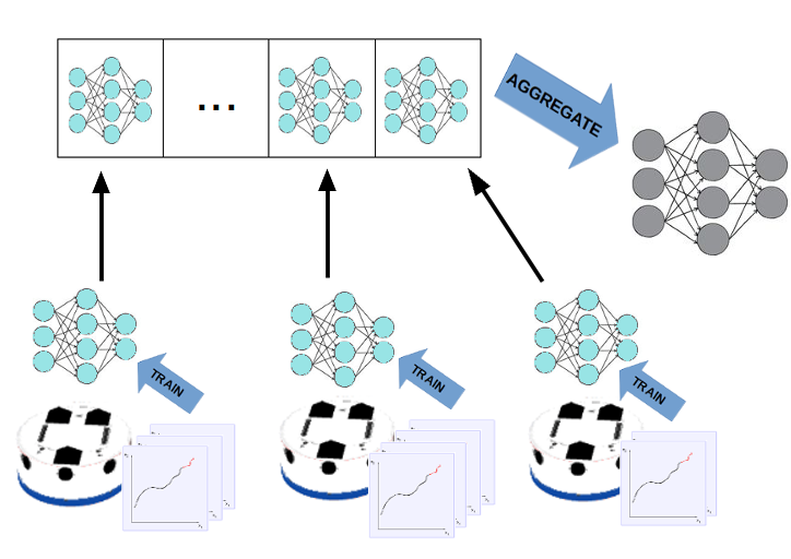
(c) Distributed Federated Learning.

Figure 2: Learning frameworks.

III PRELIMINARIES

In this section we formalize the federated learning problem and justify our application scenario.

III-A Federated Learning

In machine learning, the objective function is usually of the form:

$$\underset{\mathbf{\Theta}}{\mathrm{min}}\thinspace L(f(x;\mathbf{\Theta}),y):=\frac{1}{n}\sum_{i=1}^{n}L(f(x^{(i)};\mathbf{\Theta}),y^{(i)})$$ (1)

where the aim is to train a model $f(\cdot)$ with weights $\mathbf{\Theta}$, mapping an input $x\in\mathbb{R}^{I}$ to an output $y\in\mathbb{R}^{O}$. Using a training data set of $n$ samples $(x,y)\in\mathbb{R}^{I\times O}$, we can adjust the weights of the model to minimize a loss function $L(\cdot)$ that expresses the error between the inferred output $\hat{y}$ and the true output $y$.

Federated Learning. FL [2] is an optimization problem that considers a modified version of Equation 1 where the training examples are now stored across $K$ clients and a global server attempts to minimize a loss function obtained from aggregated local weights (Figure 2(b)). In our case, clients refer to robots that collect data. The global function that is minimized is the summation of the local losses obtained on the $k$-th robot, $L_{k}(\mathbf{\Theta})$, weighted by the number of samples observed $n_{k}$ over the total number of samples $n$ in the dataset:

$$\underset{\mathbf{\Theta}}{\mathrm{min}}\thinspace L(\mathbf{\Theta})=\underset{\mathbf{\Theta}}{\mathrm{min}}{\sum_{k=1}^{K}\frac{n_{k}}{n}\times L_{k}(\mathbf{\Theta})},$$ (2)

The local loss of the robot $L_{k}(\mathbf{\Theta})$ is similar to that in the traditional machine learning case,

$$L_{k}(\mathbf{\Theta})=\frac{1}{n_{k}}\sum_{h=1}^{n_{k}}\ell(x_{h},y_{h};\mathbf{\Theta})$$ (3)

where $\ell(x_{h},y_{h};\mathbf{\Theta})$ is the loss of the predicted model over the $n_{k}$ samples $(x_{h},y_{h})$ observed by the robot $k$, using global model parameters $\mathbf{\Theta}$.

Assumptions. FL is typically based on a number of key assumptions on the data: (i) It is non-i.i.d. (independent and identically distributed); (ii) It is stored across several clients; and (iii) It is partitioned in an imbalanced manner, resulting in clients that handle more data than others. In addition, communication among clients is assumed to be intermittent. In traditional FL the presence of a server ensures synchronization, however, as discussed in Section II, serverless settings are also possible. In this paper, we maintain all of the above assumptions. In particular, we study the effect that the presence or absence of a server has on the performance of the learning process.

III-B Application: Trajectory Forecasting

In this work we consider trajectory prediction as an application example of Flow-FL. Trajectory forecasting is typically conducted with pedestrian data. However, existing literature on trajectory forecasting [14, 15, 16] focuses on pedestrian data collected from a single point of view which is usually an overhead camera. As such, the available datasets are not easily amenable to an FL setting. To the best of our knowledge, there are no federated datasets of trajectories collected by multiple robots. For this reason, we generated a novel federated dataset from artificial navigation data in four different multi-robot settings (see Section IV-B). In future work, we will use real robots to collect motion data of real dynamic obstacles such as pedestrians.

Trajectory forecasting is a compelling problem for machine learning applications. This problem is about creating a model that allows robots to predict the trajectories of dynamic obstacles nearby within a short time horizon. Research has shown that navigation is significantly more efficient when using a machine learning model than with purely reactive methods, such as ORCA and RVO [17, 18]. While numerous neural networks have been benchmarked [14], a simple Long Short-Term Memory (LSTM) model [19] has been shown to yield the lowest Average Displacement Error on the standard datasets. Therefore, we use this model architecture in our evaluation.

IV METHODOLOGY

IV-A System Design

In a traditional FL setting, a server communicates with data-holding clients to enable training of a global ML model (see Figure 2(b)). The server does not aggregate data, as opposed to a fully centralized approach (see Figure 2(a)). However, in traditional FL, the server has the important roles of: (i) orchestrating learning rounds periodically by selecting a subset of learners and sending them model parameters; (ii) aggregating the results of a round of learning into a global model. In our approach, depicted in Figures 2(c) and 3, we replace the central server with a distributed algorithm. The scheduling of learning rounds is data-driven, and it happens when a sufficient number of robots have collected enough data. To keep the rounds sequential and distinct, a global state is maintained in a gossip-based shared memory. Model weights are written to this shared memory at the end of each round. The aggregation happens in the subsequent round, when robots with enough data pull the weights from the shared memory to instantiate their local models.

Application scenario. We consider a scenario with $K$ moving robots that communicate and track each other’s relative positions within a limited range. We tackle the problem of learning to predict the robot trajectories for a certain time horizon (see Figure 1 for examples of the robot trajectories). In our setup, robots are moving, collecting data and performing learning concurrently. This is in contrast with existing frameworks for multi-robot learning, which require some sort of synchronicity in switching through these activities. To the best of our knowledge, this is an item of novelty in our framework. In our setup, the motion behavior is determined by a pre-programmed controller. We chose well-studied swarm behaviors such as flocking [20], foraging [21], and diffusion with obstacle avoidance [22]. The data collected by the robots consists of the spatial coordinates of neighboring robots expressed in a fixed frame local to the sensing robot. A training sample is one continuous trajectory recorded for a fixed duration at regular time steps. Each robot builds its own dataset over time from its local observations.

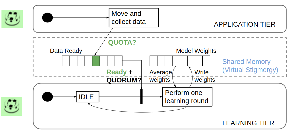
Figure 3: The state transition of the learning tier for the green robot is conditioned by the data flow of its application tier and a global state tracked in the shared memory.

State machine of the learning framework (Figure 3). The operation of the robots is organized in two tiers. The learning tier runs separately from the application tier that performs the swarm behavior. The robots start in Idle state. Each robot has knowledge of the model architecture, but it starts with the same random weights and no data.

The transition to the first learning round is conditioned by the flow of data. When a robot collects a certain quota of training samples, it marks itself as ready in the shared memory. When a sufficient number of robots have marked themselves ready, we say that a quorum has been reached and the ready robots collectively transition to the learning round. These robots, the learners, perform local training on the data they had gathered and forget their samples.

The next transition brings the robots back to the Idle state in the learning tier. The transition happens after all the learners finish sharing their new ML model weights with the rest of the swarm. Each learner shares its weights after performing one training epoch on its samples.

From now on, the transitions out of the Idle state proceed in a data-driven fashion as the first transition. However, the learning rounds start differently: in this case, the learners must first retrieve and aggregate the most recent weights from the shared memory.

Shared memory. The shared memory has two purposes: (i) It holds a global list of ready robots which is used to synchronize state transitions when the quorum of ready robots is achieved; and (ii) It stores the updated model weights in a dedicated global list. We implemented data sharing through Virtual Stigmergy (VS) [13]. VS is a lightweight, distributed tuple space designed to share a collection of (key,value) pairs. A local Lamport-clock-stamped copy of each tuple is stored on each robot. This copy is updated upon both read() and write() operations through network flooding. In this way, while the network topology changes, the data structure is kept up-to-date.

Transition mechanism. The state transitions are achieved through a barrier mechanism making use of the VS. We outline the steps for this count-based consensus protocol in Algorithm 1.

ML model architecture. The ML model used for the application is a standard architecture for time series prediction. We use one Long Short-Term Memory (LSTM) layer [19] with a hidden dimension of 16 without returning sequences, followed by a dense layer and Dropout of 0.2 . The network looks at a history of 32 prior $(x,y)$ observations (corresponding to 3.2 s) and directly outputs a prediction for the next 48 time steps (4.8 s). We used a Mean Squared Error (MSE) loss $\text{MSE}=\frac{1}{N}\sum_{i=1}^{N}(\textbf{x}_{i}-\tilde{\textbf{x}}_{i})^{2}$ as a training metric that is then optimized using RMSProp [23].

ML model aggregation. Similar to the implementation in FedAvg [2] the learners update the global list with their learned weights after performing a gradient descent step on local data. During the next time step, the new weights for the server are the average of all the learned weights on the list weighted by the number of samples encountered by each learner. McMahan et al. also found that, for large local epochs, FedAvg can plateau or diverge. They recommend either using fewer local epochs or decaying the number of local computations over time. We do not study this aspect, and let the learners perform only a single local epoch per iteration and flush this data before collecting new data during the next iteration.

Algorithm 1 Barrier - robot $k$, barrier VS $\beta_{k}$, neighbors $\mathcal{N}_{k}$

1:procedure barrier_set

2:     initialize barrier $\beta_{k}\leftarrow list()$ for robot $k$

3:     robot state $\leftarrow$ barrier_wait

4:     activate ON_BARRIER_UPDATE

5:end procedure

6:procedure on_barrier_update($\mathcal{N}_{k}$)

7:     $\mathbf{receive}\,\,\{i\}_{i\in\mathcal{N}_{k}}$ $\triangleright$ RX from neighbors

8:     if $i\not\in\beta_{k}$ then

9:         $\beta_{k}\leftarrow\beta_{k}\cup i$

10:         $\mathbf{send}\left(i\right)$ $\triangleright$ TX to neighbors

11:     end if

12:end procedure

13:procedure barrier_ready($\mathcal{N}_{k}$)

14:     $\mathbf{receive}\,\,\{i\}_{i\in\mathcal{N}_{k}}$ $\triangleright$ RX from neighbors

15:     $\beta_{k}\leftarrow\beta_{k}\cup k$

16:     if element_count($\beta_{k}$) $\geq$ threshold then

17:         robot state $\leftarrow$ next_state

18:     end if

19:     $\mathbf{send}\left(\Delta\beta_{k}\right)$ $\triangleright$ TX to neighbors

20:end procedure

IV-B Datasets

To the best of our knowledge, this paper is the first to provide an open-source federated dataset of swarm motion with information on the communication graph. We generated multiple synthetic datasets of swarm motion across four distinct behaviors using ARGoS, a realistic physics-based simulator [24].

Data format. Each behavior dataset consists of:

• A trajectory file that records the robot’s id, neighbor id, and position across time (robot id, neighbor id, t, x, y, z). Each robot records neighbor trajectories for 50,000 time steps (5,000 s). A trajectory sample, within a setup, is 100 time steps (10 s) long and is separated from other samples by an end-of-line character. Each trajectory is expressed in the local reference frame of the robot at the start of the sample recording. This is a fixed frame of reference independent of subsequent robot motion.

• A communication graph file, structured as (t, robot id, neighbor id), that logs information about the neighboring robot IDs that are in range at every time step. This information encodes the communication graph at every time step. The communication graph file is more complete than the trajectory file because when recording the trajectory file, we drop interrupted trajectories.

Parameter setting. The experimental settings are kept consistent across datasets as shown in Table I. The settings include: (i) the trajectory sampling period; (ii) additive noise for positional data on each robot neighbor sampled from a normal distribution; and (iii) wheel actuation noise, also sampled from a normal distribution. The noise parameters are rounded estimates from realistic samples taken from real-world Khepera robots. We executed the experiments for swarms with $K=\{15,60\}$ robots to enable the study of the effect of different swarm sizes.

TABLE I: Experiment settings

Parameter	Value
Trajectory duration	10 s
Communication range	2 m
Sensing range	2 m
Sensing noise $n_{k}(t)$	$n_{k}(t)\sim\mathcal{N}(0,0.01)$ m
Drive bias $e_{k}$	$e_{k}\sim\mathcal{N}(0,0.0001)$ m

Behavior types. We evaluate our methodology with four different swarm behaviors [25]: (i) Obstacle-avoidance [22] (Figure 4 top row) in a dense environment with uniformly distributed static obstacles; (ii) Foraging [21] (Figure 4 bottom row) for resources in which robots decide whether to explore or stay in the nest according to energy considerations; (iii) Phototaxis and flocking based on artificial physics [20], with a light whose position is changed to prevent stagnation; and (iv) A mixed behavior in which robots perform one of the previous behaviors depending on their location in the environment. The datasets and corresponding simulation videos can be found at https://www.nestlab.net/doku.php/papers:mrs_fl_dataset. Table II provides the total number of samples in each dataset as well as statistics about the distribution of samples between robots. The table reveals diversity across the behaviors in the number of samples collected, both total and per robot, also considering total time and 10-minute windows. In particular, the standard deviation shows how different behaviors result is different levels of imbalance in the number of samples collected by the robots.

TABLE II: Statistics for swarm motion federated datasets.

Dataset	Robots	Samples	Samples/robot		Samples/robot
					/10 min
			Mean	Stdev	Mean	Stdev
Avoidance	15	21,227	1,415	206	169	40
	60	216,582	3,610	397	429	74
Flocking	15	49,009	3,267	427	390	78
	60	333,111	5,552	436	659	112
Foraging	15	35,854	2,390	46	284	19
	60	187,304	3,122	65	371	25
Mixed	15	30,627	2,042	290	242	66
	60	174,863	2,914	89	346	29

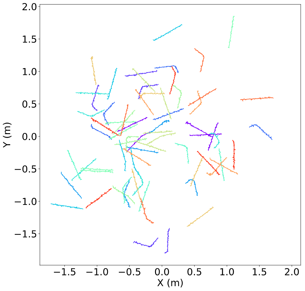
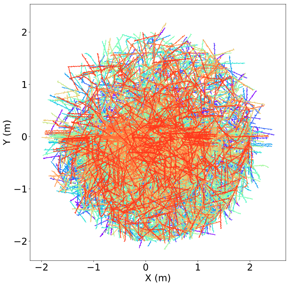
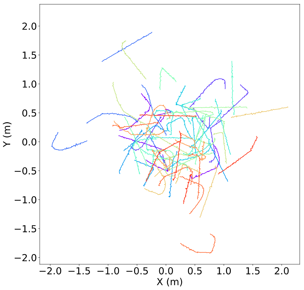
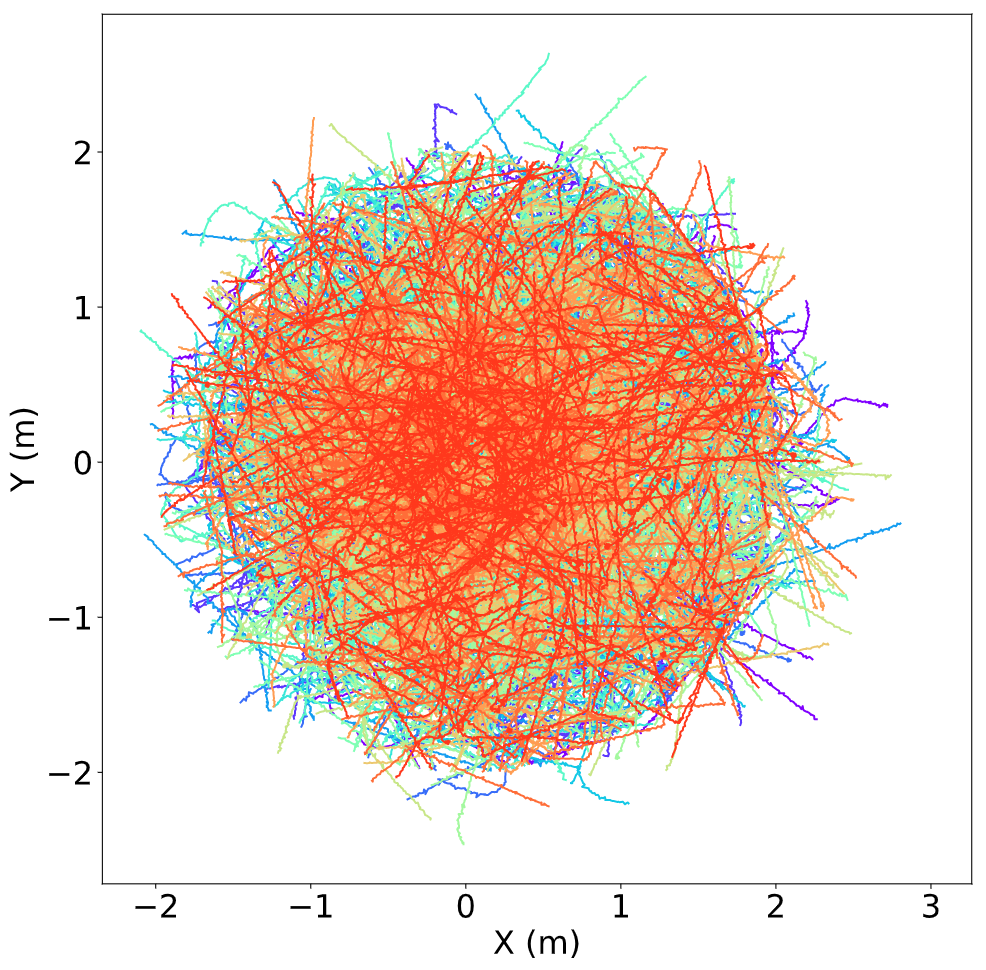
Figure 4: Avoidance (top) and foraging (bottom) for $K=15$. Left to right: increased number of displayed samples.

V EVALUATION

V-A Parameters of Interest

Quorum and quota. The main parameters of interest in our empirical study are the quorum of learners and the quota of data. These parameters condition the transition to a learning state for a subset of robots at times dictated by the data collection flow (see Figure 3). We set the quorum as a fraction $q_{F}$ of the total number of robots. We perform our study with datasets from experiments with a fixed duration of 5,000 s. Quorum and quota determine the total number of learning rounds in each study configuration as they split the data in time.

Number of robots. We also study the influence of the number of robots by using 15- and 60-robot datasets. We expect this parameter to act on different aspects of multi-robot communication and learning as it changes: (i) the total amount and frequency of data collected, which changes the time between learning rounds (Section V-C); (ii) the robot communication network size and topology, which change the latency of the shared data structure and affect the timing of learning rounds (Section V-C); (iii) the partitioning of federated data across clients, which influences the convergence rate (Section V-B).

Federated datasets. We use multiple federated datasets detailed in Section IV-B with different behaviors (see Figure 4). We provide and compare results for these 8 datasets.

Learning hyperparameters. We set the learning hyperparameters for the local machine learning model as detailed in Section IV-A. In terms of standard FL hyperparameters, we set number of local epochs $E$ to 1. Increasing $E$ reduces communication overhead at the cost of increased individual computational load. McMahan et al. [2] provide an empirical study of the effect of this parameter. They show that high values of $E$ can lead the FL algorithm to diverge. In the same paper, McMahan et al. also vary the quorum fraction but refer to it as client fraction. In this paper, we focus on the effect of controlling the data flow through $q_{F}$ and quota rather than changing the amount of local computation through $E$.

Dataset split. To separate our data into training/validation/test samples, we proceed in the following way: we take 80 % (first 4,000 s) of the experiment data for training and validation and keep the remaining for testing; within a learning round, each learner splits the data into a set of training samples (the first 80 % of trajectories), and validation samples (the last 20 % of trajectories). We verified that behaviors do not change at the end of the experiment so as to have an appropriate testing set.

TABLE III: Evaluation parameters

Parameter	Value
Number of robots $K$	$\{15,60\}$ robots
Quorum fraction $q_{F}$	$\{0.2,0.6\}$
Quorum	$q_{F}\cdot K$ robots
Quota	$\{20,60\}$ samples
Local epochs $E$	1

V-B Convergence Analysis

An important aspect of our FL framework is the effect of scheduling rounds according to quorum and quota on the learning convergence. We want to study the following aspects empirically across several datasets:

• which $(q_{F},$ quota) configuration requires the least learning rounds to achieve convergence. Reducing the number of learning rounds reduces communication rounds thereby decreasing communication overhead;

• which $(q_{F},$ quota) configuration requires data spread across the least time steps to achieve convergence. Reducing the number of steps gives us a final model earlier on in the experiment;

• which $(q_{F},$ quota) configuration gives us the best trade-off between the two above situations.

Varying quorum and quota is effectively re-partitioning the data in time within the same dataset. With respect to learning, this affects the rate of model updates as well as the number of participating clients $\bar{K}$ and the number of local examples $n_{k}$ used for the update at each round.

We study the effect of $(q_{F}$, quota) on the federated validation loss $L(\mathbf{\Theta})$ from Equation 2. To make the comparison fair with Flow-FL, we implemented a data-driven FL approach with a server scheduling rounds according to $q_{F}$ and quota, i.e., starting a round as soon as $q_{F}\cdot K$ robots have a quota of samples. In the distributed version Flow-FL, the learning rounds are scheduled the same way, but they occur with a delay after the quorum/quota condition is met. This delay is due to the latency imposed by the update of the shared data structure. Thus, a different number of learners may qualify at the same time. To compare convergence in a consistent way, we define the stopping round as the round where the windowed average of loss changes less than a threshold of $0.0001$. The averaging window was set to 5 rounds.

Discussion. Figure 5 shows the federated validation loss curves. We also show the centralized validation loss as a baseline that uses all the data collected by the end of the experiment at once. To compare the loss over iterations, we show epochs for the centralized loss and learning rounds for the federated loss. We include as many epochs for the baseline as the number of learning rounds in Flow-FL. Table IV reports the final loss value and stopping points for all the behaviors. The final loss is similar across configurations, but it tends to increase as the total number of iterations decreases. With higher $(q_{F}$, quota), we have fewer learning rounds because it takes more data to move to the next training round. We also note fewer oscillations of the learning curve with higher $(q_{F}$, quota).

Stopping rounds and times. Table IV shows the lowest stopping rounds and times across configurations in bold:

• We see that, while changing across behaviors, the lowest number of learning rounds occurs with higher thresholds of ($q_{F}$, quota) than the minimum $(0.2,20)$;

• We get lower numbers of time steps at stopping with lower thresholds for ($q_{F}$, quota). However, the stopping criterion sometimes selected an early stopping round with some oscillations occurring later in the curve. Those instances are denoted by an asterisk.

• The best trade-off between number of rounds and time steps is at $(q_{F}$, quota) $=(0.2,60)$.

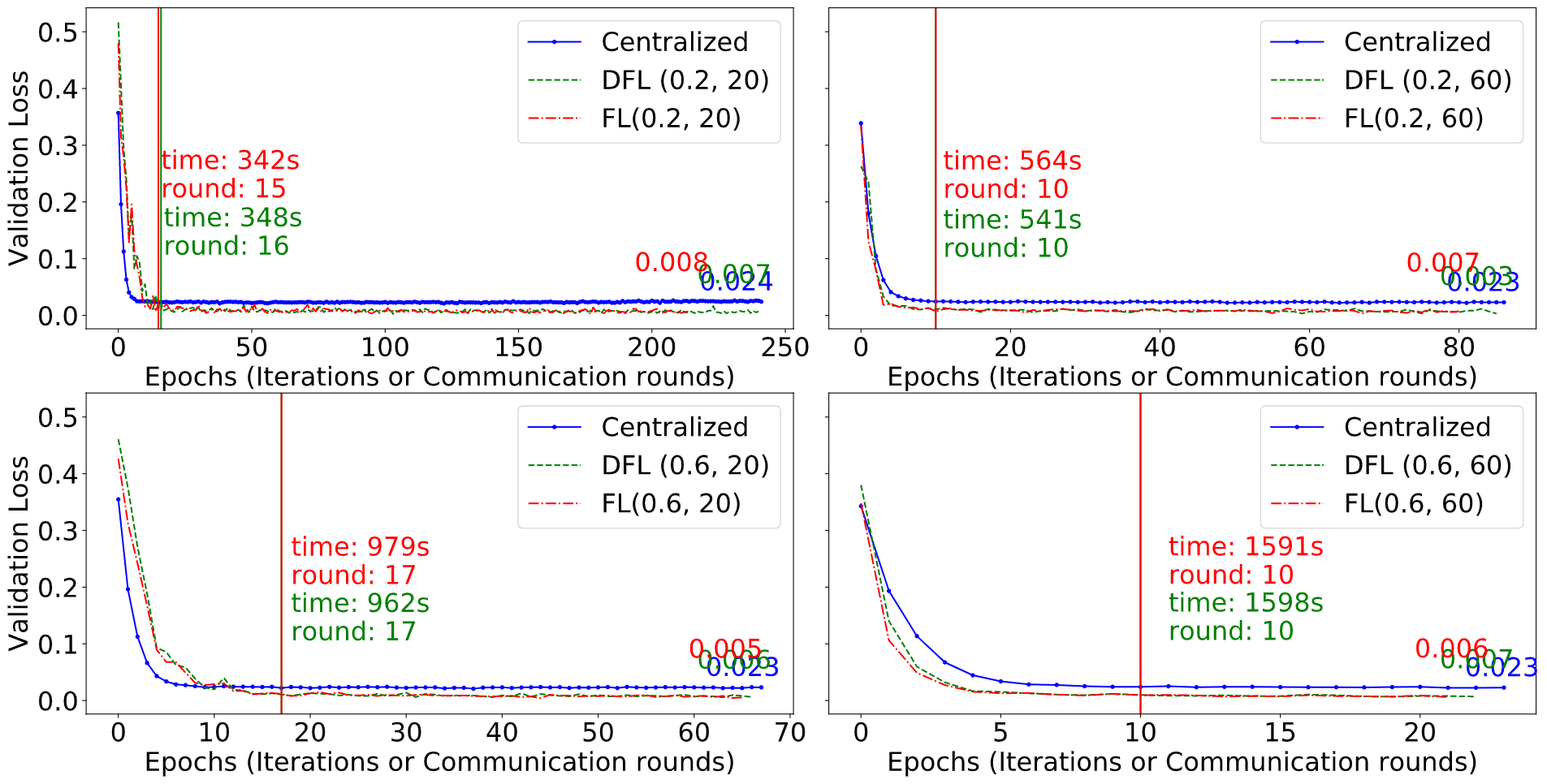
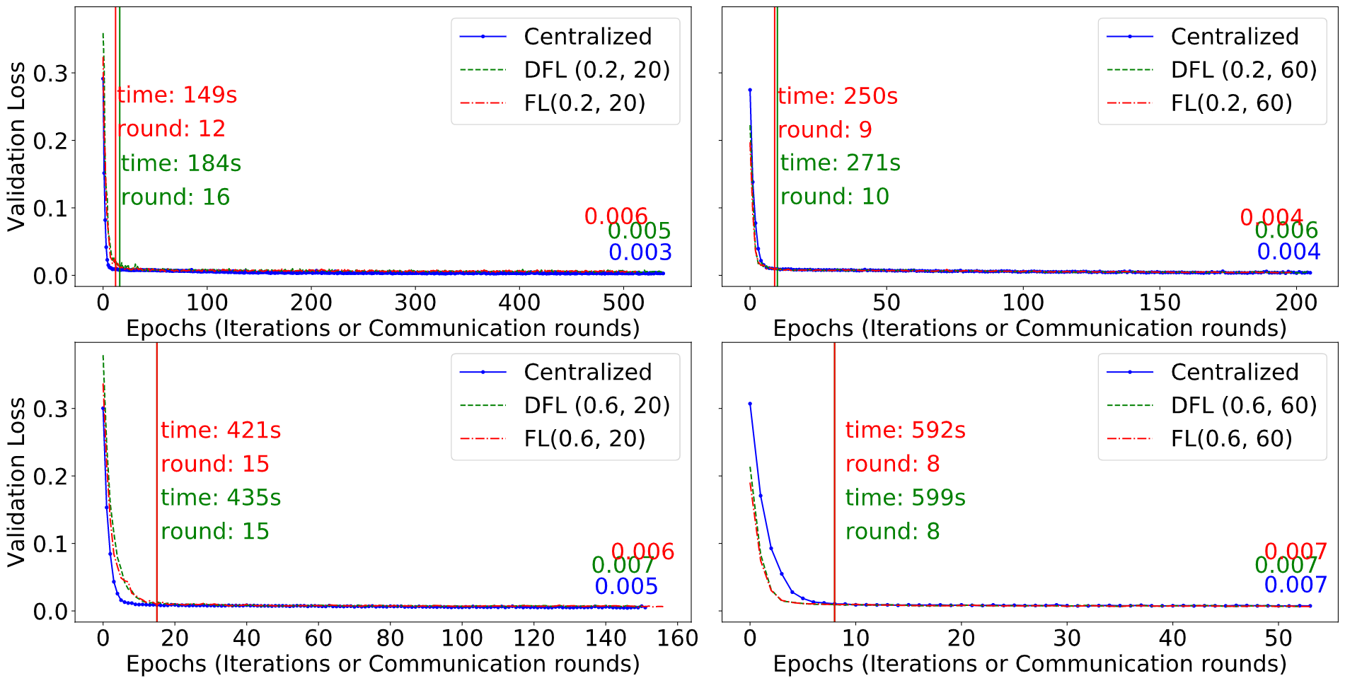
Figure 5: Validation loss $L(\mathbf{\Theta})$ for the avoidance behavior with 15 (left), 60 (right) robots (DFL=Flow-FL).

TABLE IV: Convergence data across quorums and quotas for different behaviors ($K=60$).

($q_{F}$, quota)		(0.2 20)	(0.2, 60)	(0.6, 20)	(0.6, 60)
Flocking
Validation loss	C	0.002	0.002	0.002	0.002
	FL	0.002	0.001	0.001	0.001
	Flow-FL	0.002	0.002	0.002	0.002
Stopping round	FL	17	8	16	6
	Flow-FL	17	8	13	8
Stopping time(s)	FL	134*	157	297	292
	Flow-FL	136*	157	247	402
Foraging
Validation loss	C	0.011	0.011	0.012	0.016
	FL	0.014	0.013	0.017	0.014
	Flow-FL	0.012	0.013	0.016	0.015
Stopping round	FL	21	7	13	8
	Flow-FL	15	10	16	7
Stopping time(s)	FL	257	257	448	731
	Flow-FL	192	326	562	636
Avoidance
Validation loss	C	0.003	0.004	0.005	0.007
	FL	0.006	0.004	0.006	0.007
	Flow-FL	0.005	0.006	0.007	0.007
Stopping round	FL	12	9	15	8
	Flow-FL	16	10	15	8
Stopping time(s)	FL	149*	250	421	592
	Flow-FL	184*	271	435	599
Mixed
Validation loss	C	0.006	0.007	0.009	0.012
	FL	0.008	0.008	0.010	0.010
	Flow-FL	0.010	0.009	0.012	0.011
Stopping round	FL	20	8	19	8
	Flow-FL	16	8	15	8
Stopping time(s)	FL	232	242	611	705
	Flow-FL	192	241	503	711

V-C Learning Round Timing

The scheduling of learning rounds is data-driven both in our version of FL and in Flow-FL. The time between learning rounds increases when we increase either the learner quorum or the sample quota. Figure 6 shows the time between rounds over the duration of the experiment. This time depends on the flow of data in the experiment and the length of the time series we consider as samples. The graph shows that, for a given (quorum,quota) setting, the inter-round duration is similar between FL and Flow-FL. This is due to the short time spent by the robots in the barrier with Flow-FL. With $K=15$, the average time spent in the barrier is 15 time steps (1.5 s) and, with $K=60$, it is 51 time steps (5.1 s). A wider empirical study of the latency of virtual stigmergy is reported in [13].

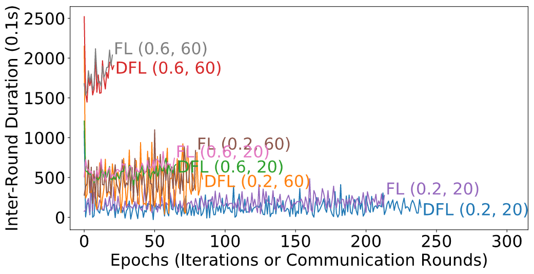
Figure 6: Timing for avoidance with 15 robots (DFL=Flow-FL).

V-D Prediction Quality

We quantify the prediction quality of trajectory forecasting based on two metrics: (i) The Average Displacement Error (ADE) in Equation 4, that is a summation of the L2-norm between the ground truth $\mathbf{y_{i,t}}$ and the predicted trajectory $\mathbf{\tilde{y}_{i,t}}$ over the predicted horizon $T$ for all trajectory samples $N_{\text{traj}}$; (ii) The Final Displacement Error (FDE) in Equation 5 which is the summation of the L2-norm of the final positions between the predicted $\mathbf{\tilde{y}_{i,T}}$ and the ground truth $\mathbf{y_{i,T}}$ over all trajectory samples.

$$\text{ADE}=\frac{1}{N_{\text{traj}}\cdot~{}T}\sum_{i=1}^{N_{\text{traj}}}\sum_{t=1}^{T}\|(\mathbf{y}_{i,t}-\mathbf{\tilde{y}}_{i,t})\|$$ (4)

$$\text{FDE}=\frac{1}{N_{\text{traj}}}\sum_{i=1}^{N_{\text{traj}}}\|(\mathbf{y}_{i,t=T}-\mathbf{\tilde{y}}_{i,t=T})\|$$ (5)

TABLE V: Trajectory reconstruction across quorums and quotas for different behaviors. ($K=60$)

$\mathbf{(q_{F},}$		(0.2,	(0.2,	(0.6,	(0.6,
quota)		20)	60)	20)	60)
Flocking
FDE (m)	Centralized	0.08$\pm$0.04	0.08$\pm$0.04	0.08$\pm$0.04	0.09$\pm$0.04
	FL	0.08$\pm$0.04	0.08$\pm$0.04	0.09$\pm$0.05	0.08$\pm$0.04
	Flow-FL	0.09$\pm$0.05	0.08$\pm$0.04	0.09$\pm$0.05	0.09$\pm$0.04
ADE (m)	Centralized	0.05$\pm$0.03	0.05$\pm$0.03	0.05$\pm$0.03	0.05$\pm$0.03
	FL	0.05$\pm$0.03	0.05$\pm$0.03	0.05$\pm$0.03	0.05$\pm$0.03
	Flow-FL	0.06$\pm$0.03	0.05$\pm$0.03	0.06$\pm$0.03	0.05$\pm$0.03
Foraging
FDE (m)	Centralized	0.22$\pm$0.11	0.23$\pm$0.11	0.23$\pm$0.11	0.27$\pm$0.13
	FL	0.25$\pm$0.12	0.23$\pm$0.12	0.27$\pm$0.13	0.25$\pm$0.12
	Flow-FL	0.24$\pm$0.12	0.23$\pm$0.12	0.27$\pm$0.13	0.25$\pm$0.12
ADE (m)	Centralized	0.11$\pm$0.05	0.12$\pm$0.05	0.12$\pm$0.06	0.14$\pm$0.06
	FL	0.13$\pm$0.06	0.12$\pm$0.06	0.14$\pm$0.07	0.13$\pm$0.06
	Flow-FL	0.13$\pm$0.06	0.12$\pm$0.06	0.14$\pm$0.07	0.13$\pm$0.06
Avoidance
FDE (m)	Centralized	0.11$\pm$0.05	0.13$\pm$0.05	0.15$\pm$0.06	0.19$\pm$0.06
	FL	0.17$\pm$0.06	0.14$\pm$0.05	0.19$\pm$0.06	0.18$\pm$0.06
	Flow-FL	0.16$\pm$0.06	0.14$\pm$0.05	0.19$\pm$0.06	0.18$\pm$0.07
ADE (m)	Centralized	0.06$\pm$0.02	0.07$\pm$0.03	0.08$\pm$0.03	0.10$\pm$0.04
	FL	0.09$\pm$0.04	0.07$\pm$0.03	0.10$\pm$0.04	0.10$\pm$0.04
	Flow-FL	0.08$\pm$0.03	0.07$\pm$0.03	0.10$\pm$0.04	0.10$\pm$0.04
Mixed
FDE (m)	Centralized	0.15$\pm$0.10	0.17$\pm$0.11	0.18$\pm$0.12	0.21$\pm$0.15
	FL	0.21$\pm$0.14	0.18$\pm$0.13	0.24$\pm$0.17	0.21$\pm$0.15
	Flow-FL	0.20$\pm$0.14	0.18$\pm$0.12	0.24$\pm$0.17	0.21$\pm$0.14
ADE (m)	Centralized	0.08$\pm$0.05	0.09$\pm$0.05	0.10$\pm$0.06	0.11$\pm$0.07
	FL	0.11$\pm$0.07	0.09$\pm$0.06	0.13$\pm$0.09	0.11$\pm$0.07
	Flow-FL	0.11$\pm$0.07	0.09$\pm$0.06	0.13$\pm$0.09	0.11$\pm$0.07

We report the ADE, FDE metric results in Table V to 2 decimal places since this corresponds to centimeter-level granularity. We maintain consistency across the evaluations in the case of centralized training by setting the number of epochs trained to the number of rounds performed by Flow-FL for the (quorum, quota) pair. We note that trajectories are forecast similarly by the three methods across all four behaviors with no notable differences. We identify that, in general, reconstructing flocking trajectories which are goal-oriented to a light source is much easier than reconstructing foraging or avoidance trajectories which need additional context information from neighbors (such as distance between neighbors in the case of obstacle avoidance, or location of resources/the nest for foraging). The generated output trajectories are shown in Figure 7. Data such as a robot’s motion model, higher-derivative information (such as velocity), or a particular agent’s goals would help robustly predicting turning or in some cases matching the distance traveled by a robot (even though the orientations are predicted accurately). These improvements are out of the scope of our work.

Figure 7: Fifteen trajectories predicted using Flow-FL for one robot with mixed behaviors in a swarm for $K=60$.

VI CONCLUSIONS

In this work, we explore the design space of Federated Learning in a robotics setting. Our study includes two versions of Federated Learning (one server-dependent and one serverless), and one centralized approach as our baseline. We provide a practical realization of fully distributed Federated Learning, Flow-FL, in a multi-robot setting. We propose a way to schedule model updates based on data flow by considering two parameters: the quota, i.e., the minimum number of data samples for a robot to qualify for a model update, and the quorum, i.e., the minimum number of robots to start a learning round.

We studied the role of several parameters of practical relevance, such as staggered online data collection, number of participating robots, and time delays introduced by decentralization. As we envision our approach to be useful in learning dynamic spatio-temporal datasets, we considered a well-known case study with compelling dynamics in both space and time: trajectory forecasting. Due to the lack of usable datasets in the literature, we created the first federated dataset from artificial data collected from a representative set of multi-robot behaviors.

In future work, we will apply Flow-FL to real-world pedestrian data collected with a team of robots. In addition, we will study the role of the communication topology in keeping communication delays limited when the number of robots increases. Finally, we will study the role of aggressive communication loss on the convergence of Flow-FL.

References

- [1] M. Brambilla, E. Ferrante, M. Birattari, and M. Dorigo, “Swarm robotics: A review from the swarm engineering perspective,” Swarm Intelligence, vol. 7, no. 1, pp. 1–41, 2013.
- [2] B. McMahan, E. Moore, D. Ramage, and S. Hampson, “Communication-efficient learning of deep networks from decentralized data,” in Proceedings of the 20th International Conference on Artificial Intelligence and Statistics (AISTATS).
- [3] P. Kairouz, H. B. McMahan, B. Avent, A. Bellet, M. Bennis, A. N. Bhagoji, K. Bonawitz, Z. Charles, G. Cormode, R. Cummings et al., “Advances and open problems in federated learning,” arXiv preprint arXiv:1912.04977, 2019.
- [4] M. Everett, Y. F. Chen, and J. P. How, “Collision avoidance in pedestrian-rich environments with deep reinforcement learning,” 2020.
- [5] D. Peteiro-Barral and B. Guijarro-Berdiñas, “A survey of methods for distributed machine learning,” Progress in Artificial Intelligence, vol. 2, no. 1, pp. 1–11, 2013.
- [6] J. Verbraeken, M. Wolting, J. Katzy, J. Kloppenburg, T. Verbelen, and J. S. Rellermeyer, “A Survey on Distributed Machine Learning,” ACM Computing Surveys, vol. 53, pp. 1–33.
- [7] S. Savazzi, M. Nicoli, and V. Rampa, “Federated Learning with Cooperating Devices: A Consensus Approach for Massive IoT Networks,” IEEE Internet Things J., pp. 1–1, 2020, arXiv: 1912.13163. [Online]. Available: http://arxiv.org/abs/1912.13163
- [8] A. Lalitha, S. Shekhar, T. Javidi, and F. Koushanfar, “Fully decentralized federated learning,” in Third workshop on Bayesian Deep Learning (NeurIPS), 2018.
- [9] A. Lalitha, O. C. Kilinc, T. Javidi, and F. Koushanfar, “Peer-to-peer federated learning on graphs,” arXiv preprint arXiv:1901.11173, 2019.
- [10] J. George and P. Gurram, “Distributed deep learning with event-triggered communication,” arXiv preprint arXiv:1909.05020, 2019.
- [11] M. Shapiro, N. Preguiça, C. Baquero, and M. Zawirski, “Conflict-free replicated data types,” in Symposium on Self-Stabilizing Systems. Springer, 2011, pp. 386–400.
- [12] P. Ramanan, K. Nakayama, and R. Sharma, “Baffle: Blockchain based aggregator free federated learning,” arXiv preprint arXiv:1909.07452, 2019.
- [13] C. Pinciroli, A. Lee-Brown, and G. Beltrame, “A tuple space for data sharing in robot swarms,” in Proceedings of the 9th EAI International Conference on Bio-inspired Information and Communications Technologies (formerly BIONETICS). ICST (Institute for Computer Sciences, Social-Informatics and …, 2016, pp. 287–294.
- [14] A. Sadeghian, V. Kosaraju, A. Gupta, S. Savarese, and A. Alahi, “Trajnet: Towards a benchmark for human trajectory prediction,” arXiv preprint, 2018.
- [15] S. Becker, R. Hug, W. Hübner, and M. Arens, “An evaluation of trajectory prediction approaches and notes on the trajnet benchmark,” 2018.
- [16] I. Gilitschenski, G. Rosman, A. Gupta, S. Karaman, and D. Rus, “Deep context maps: Agent trajectory prediction using location-specific latent maps,” IEEE Robotics and Automation Letters, vol. 5, no. 4, p. 5097–5104, Oct 2020. [Online]. Available: http://dx.doi.org/10.1109/LRA.2020.3004800
- [17] J. van den Berg, Ming Lin, and D. Manocha, “Reciprocal velocity obstacles for real-time multi-agent navigation,” in 2008 IEEE International Conference on Robotics and Automation, 2008, pp. 1928–1935.
- [18] J. van den Berg, S. J. Guy, M. Lin, and D. Manocha, “Reciprocal n-body collision avoidance,” in Robotics Research, C. Pradalier, R. Siegwart, and G. Hirzinger, Eds., 2011, pp. 3–19.
- [19] S. Hochreiter and J. Schmidhuber, “Long short-term memory,” Neural Comput., vol. 9, no. 8, p. 1735–1780, Nov. 1997. [Online]. Available: https://doi.org/10.1162/neco.1997.9.8.1735
- [20] W. M. Spears, R. Heil, and D. Zarzhitsky, “Artificial physics for mobile robot formations,” in 2005 IEEE International Conference on Systems, Man and Cybernetics, vol. 3, 2005, pp. 2287–2292 Vol. 3.
- [21] W. Liu, A. F. T. Winfield, J. Sa, J. Chen, and L. Dou, “Towards energy optimization: Emergent task allocation in a swarm of foraging robots,” Adaptive Behavior, vol. 15, no. 3, pp. 289–305, 2007. [Online]. Available: https://doi.org/10.1177/1059712307082088
- [22] A. Howard, M. Mataric, and G. Sukhatme, “Mobile sensor network deployment using potential fields: A distributed, scalable solution to the area coverage problem,” in DARS, 2002.
- [23] T. Tieleman and G. Hinton, “Lecture 6.5-rmsprop: Divide the gradient by a running average of its recent magnitude,” COURSERA: Neural networks for machine learning, vol. 4, no. 2, pp. 26–31, 2012.
- [24] C. Pinciroli, V. Trianni, R. O’Grady, G. Pini, A. Brutschy, M. Brambilla, N. Mathews, E. Ferrante, G. Di Caro, F. Ducatelle, M. Birattari, L. M. Gambardella, and M. Dorigo, “ARGoS: a modular, parallel, multi-engine simulator for multi-robot systems,” Swarm Intelligence, vol. 6, no. 4, pp. 271–295, 2012.
- [25] “ARGoS large-scale robot simulations: examples,” https://www.argos-sim.info/examples.php, accessed: 2020-04-15.