Importance of mirror modes in binary black hole ringdown waveform

Abstract

The post-merger signal in binary black hole merger is described by linear, black-hole perturbation theory. Historically, this has been modeled using the dominant positive-frequency (corotating), fundamental mode. Recently, there has been a renewed effort in modeling the post-merger waveform using higher, positive-frequency overtones in an attempt to achieve greater accuracy in describing the waveform at earlier times using linear perturbation theory. It has been shown that the inclusion of higher overtones can shift the linear regime to the peak of $(l,m)=(2,2)$ spherical harmonic mode. In this work, we show that the inclusion of negative-frequency (counterrotating) modes, called ‘mirror’ modes, extends the validity of linear perturbation theory to even earlier times, with far lower systematic uncertainties in the model in recovering remnant parameters at these early times. A good description of the signal at early times also enables for a greater signal-to-noise ratio to be accumulated in the ringdown phase, thereby, allowing for a more accurate measurement of remnant parameters and tests of general relativity.

I Introduction

A perturbed black hole (BH) settles down to a stationary state by the emission of gravitational waves. At late times, when the perturbations are small and backreaction is not substantial, emitted gravitational waves form a discrete spectrum of complex frequencies called quasi-normal modes (QNMs) (Vishveshwara, 1970), sometimes referred to as the ringdown signal. For a Kerr BH, QNMs are completely specified by its mass $M_{f}$ and dimensionless spin $a_{f}$. This is a consequence of the ‘no-hair’ theorem (Misner et al., 1973). For a given angular mode $(l,m)$, there are a countably infinite number of QNMs ($\omega_{lmn}\in\mathbb{C}$) characterized by their overtone index ($n=0,1,2,...$). The overtone numbers are assigned in decreasing order of damping times, i.e., the lowest overtone number ($n=0$) has the largest damping time and is, therefore, the longest lived. It then follows that, if one takes the starting time of the ringdown to be at a late enough time after merger, then all the higher overtones would have decayed sufficiently so that the ringdown signal can be described by a single overtone.

The information about the nature of the initial perturbation is contained in the complex excitation amplitude of each QNM. For a binary black hole (BBH) merger, then, the excitation amplitudes, in general, depend on the binary parameters like the mass ratio ($q$), the spin angular momenta of the two component BHs ($\vec{s_{1}}$, $\vec{s_{2}}$), and the eccentricities of the binary orbit ($e_{1}$, $e_{2}$).

Historically, in gravitational wave data analysis, the start time for ringdown was choosen so that not only the non-linearities had died down but also the higher overtones had sufficient time to decay. This made it possible for ringdown to be modeled using only the most dominant QNM (Flanagan and Hughes, 1998). Recently, however, there have been efforts to model the ringdown signal using higher overtones (Giesler et al., 2019; Ota and Chirenti, 2020) by starting the ringdown at earlier times when the contribution of the higher overtones to the ringdown signal is still significant. This has mostly been due to a three-fold reason.

First, most of the BBH mergers observed by LIGO/Virgo (Aasi et al., 2015; Acernese et al., 2015) have nearly equal masses and small spins (Abbott et al., 2019). For a non-spinning, equal mass binary, the next dominant mode after $(l,m)=(2,2)$ is $(l,m)=(3,2)$ whose amplitude is a few percent compared to the dominant mode (Kamaretsos et al., 2012; Borhanian et al., 2019). For a consistency test of ‘no-hair’ theorem, one determines the mass and spin of the perturbed BH using the dominant mode (Echeverria, 1989) and uses these estimates to determine the oscillation frequency and damping time of a subdominant mode. One then checks for its consistency with the measured value of the oscillation frequency and damping time of the subdominant mode (Dreyer et al., 2004). For the current detector sensitivities and the BBH mergers we have observed so far, neither is this subdominant mode detectable nor is the frequency and damping time of the mode resolvable (Carullo et al., 2019; Brito et al., 2018) from the ringdown signal alone. Higher overtones are excited even for non-spinning, equal mass mergers and, therefore, measurement of the overtone frequencies and damping times can be used for testing the ‘no-hair’ theorem (Isi et al., 2019).

Secondly, including overtones in a ringdown model can shift the start time of ringdown to earlier times and can therefore increase the signal-to-noise (SNR) contained in the ringdown. Indeed, Giesler et al. (2019) showed that including up to $n=7$ overtones can shift the start time of ringdown to the peak of $h_{22}$ mode.

Finally, LISA could observe BBH mergers with total mass greater than $10^{8}M_{\odot}$, which would have a very small or no inspiral part (Kamaretsos et al., 2012). Having a ringdown model where multiple excitation amplitudes have been mapped to progenitor parameters can, then, be used to determine the parameters of the binaries.

There have been numerous studies in literature that model the ringdown phase of a BBH merger signal using higher angular modes (Kamaretsos et al., 2012; London et al., 2014; Baibhav et al., 2018; London, 2018). Other studies model the ringdown phase using higher overtones (Giesler et al., 2019; Ota and Chirenti, 2020). Cook (2020) does a multimode fitting of the ringdown phase including higher overtones. The effective one-body (EOB) formalism has modeled ringdown using a superposition of QNMs and psudomodes (modes that are not QNMs) (Buonanno et al., 2007; Pan et al., 2014; Taracchini et al., 2014; Babak et al., 2017). For a discussion on some of these studies, see Giesler et al. (2019).

In all of these studies, the ringdown is modeled using only the positive-frequency (corotating) part of the QNM spectrum. London et al. (2014) do look for negative-frequency modes using their greedy-OLS algorithm but do not find them to be significantly excited for non-spinning binaries. Jiménez Forteza et al. (2020) fit negative-frequency modes to a BBH merger signal for an $n=1$ overtone model and find that the lower-order counterrotating modes are not significantly excited. Hughes et al. (2019) and Lim et al. (2019) numerically solve the Teukolsky equation for a point particle infall into a Kerr BH and find negative-frequency modes are excited.

We will refer to the negative-frequency modes as ‘mirror’ modes and positive-frequency modes as ‘regular’ modes from hereon. For a BBH merger there is no reason, apriori, for the gravitational waves to consist of regular modes alone (see Berti et al. (2006) for more discussion). For the mirror modes to be omitted from ringdown waveforms consistently (especially ones including higher overtones), it has to be shown that the excitation amplitudes for these modes are much smaller than regular modes. Alternatively, one can argue that these mirror modes start at an earlier time than the regular modes and owing to their smaller damping times than their corresponding regular modes, they decay away before the ringdown starts for the (dominant) regular modes.

In this paper, we study the effect of including mirror modes in a gravitational waveform. We fit the complex excitation amplitudes to numerical relativity (NR) waveforms and show that including mirror modes in a ringdown waveform improves the fits to NR waveforms at all times in the ringdown regime. The improvement in fits is especially prominent at times before the peak of the $(l,m)=(2,2)$ spherical harmonic mode. We study the systematics of the modeling to determine if the improvement in the fits to NR waveforms is due to the presence of mirror modes in the gravitational waveform. An alternative reasoning for the enhancement of the fits could be that the additional free parameters introduced in the model due to the inclusion of mirror modes acts as basis functions and fit to some of the non-linearities in the waveform, especially at early times.

We note that most of the metrics used in this study have been introduced in Giesler et al. (2019) and Bhagwat et al. (2020) to study the importance of including higher (regular) overtones to a ringdown model. We will use their model as a reference and compare the results of our model against theirs.

Our goal is to improve the theoretical modeling of ringdown waveforms. We make the case that including mirror modes in a ringdown model give better estimates of the remnant parameters at times before the peak of the $(l,m)=(2,2)$ spherical harmonic mode. We point out that the detectability and resolvability of mirror modes is beyond the scope of this paper (see Bhagwat et al. (2020); Cabero et al. (2020); Isi et al. (2019) for a discussion on detecting higher angular modes and overtones). The start time of ringdown has also been a contentious topic in the literature and we refer the interested reader to Kamaretsos et al. (2012); Nollert (1999); Berti et al. (2007); Baibhav et al. (2018); Carullo et al. (2018) for a discussion on the different choices that have been made in the literature.

The paper is organised as follows. In section II we introduce the ringdown model and lay down the assumptions and approximations used. In section III we show our results and discuss modeling systematics. In section IV we conclude by highlighting the main results of the paper and discuss some issues with a pure ringdown model.

II Binary black hole ringdown waveform

The gravitational waves emitted by a perturbed Kerr BH of mass $M_{f}$ and spin $a_{f}$ as observed by an observer at a large distance $r$ is given by (Press and Teukolsky, 1973),

$$h(t)=h_{+}-ih_{\times}=\frac{M_{f}}{r}\sum_{lmn}\mathcal{C}_{lmn}e^{-i\omega_{lmn}t}\prescript{}{-2}{S}_{lm}(\Omega,a_{f}\omega_{lmn}),$$ (1)

where $\mathcal{C}_{lmn}=\mathcal{A}_{lmn}e^{-i\phi_{lmn}}$ are the complex excitation amplitudes, $t$ is the retarted time at null infinity, and $\Omega$ is the coordinate on a sphere $(\theta,\phi)$. The complex $\omega_{lmn}\equiv\omega_{lmn}(M_{f},a_{f})$ are the QNM frequencies as determined by perturbation theory. The complex angular functions $\prescript{}{-2}{S}_{lm}(\Omega,a_{f}\omega_{lmn})$ are the $-2$ spin-weighted spheroidal harmonic functions under which the perturbation equations of a Kerr BH decompose into a radial and angular part. They reduce to $-2$ spin-weighted spherical harmonic functions $\prescript{}{-2}{Y}_{lm}(\Omega)$ in the Schwarzschild BH case ($a_{f}=0$).

The perturbation of a Kerr BH is described by the Teukolsky equation (Teukolsky, 1973). The Teukolsky equation is a second order differential equation and, therefore, for a given angular mode $(l,m)$ and overtone number $n$, there are two linearly independent solutions. For a perturbed Schwarzschild black hole, due to the spherical symmetry of the background, if $\omega_{lmn}$ is one of the solutions, the second linearly independent solution is given by $-\omega_{lmn}^{*}$, i.e., positive- and negative-oscillation frequency solutions have the same damping time. For a Kerr black hole there is no such simple relationship between the two solutions because of the reduced symmetry of the system. One still has positive- and negative-oscillation frequency solutions, though, with the damping times of the positive oscilaltion frequency solution always larger than that of the corresponding negative oscillation frequency solution (see Fig. 1 for an example). The azimuthal symmetry of the Kerr background does, however, separate the angular part of the perturbation equations in terms of $-2$ spin-weighted spheroidal harmonics, with the radial equations obeying the following symmetry relations:

$$\omega_{lmn}=-\omega_{l-mn}^{*}\,,\;\;\;\;\;\;A_{lmn}=A_{l-mn}^{*}$$ (2)

where $A_{lmn}$ are the angular separation constants.

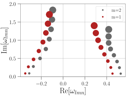
Figure 1: QNM frequencies of the first 8 overtones ($n=0,1,2,...,7$) for $l=2$ and $m>0$ for a Kerr BH with dimensionless spin $a_{f}=0.69M$ with larger flecks denoting higher overtones. Notice that the damping time of the negative-oscillation frequency solution is always shorter than its corresponding positive-oscillation frequency solution. The QNM frequencies for $m<0$ can be easily worked out using Eq. (2).

A gravitational waveform, in general, is therefore a linear combination of the two solutions and is given by,

$$\begin{split}h(t)=h_{+}-ih_{\times}=&\frac{M_{f}}{r}\sum_{lmn}[\mathcal{C}_{lmn}e^{-i\omega_{lmn}t}\prescript{}{-2}{S}_{lm}(\Omega,a_{f}\omega_{lmn})\\ &+\mathcal{C}_{lmn}^{\prime}e^{-i\omega_{lmn}^{\prime}t}\prescript{}{-2}{S}_{lm}^{\prime}(\Omega^{\prime},a_{f}\omega_{lmn})]\\ \end{split}$$ (3)

where $\Omega^{\prime}=(\pi-\theta,\phi)$.

Equation (3) can be simplified using the symmetry relation Eq. (2) to give

$$\begin{split}h(t)=h_{+}-ih_{\times}=&\frac{M_{f}}{r}\sum_{lmn}[\mathcal{C}_{lmn}e^{-i\omega_{lmn}t}\prescript{}{-2}{S}_{lm}(\Omega,a_{f}\omega_{lmn})\\ &+\mathcal{C}_{lmn}^{\prime}e^{i\omega_{l-mn}^{*}t}\prescript{}{-2}{S}_{l-m}^{*}(\Omega^{\prime},a_{f}\omega_{lmn})]\end{split}$$ (4)

Numerical relativity simulations, in general, decompose the angular part of the waveform in spherical harmonic functions and the ringdown part can be written as

$$h(t)=h_{+}-ih_{\times}=\frac{M_{f}}{r}\sum_{lm}h_{lm}(t)\prescript{}{-2}{Y}_{lm}(\Omega)$$ (5)

In order to comapre an NR waveform to a perturbation theory ringdown waveform, we have to expand the spheroidal harmonic functions in a basis of spherical hamonics.

The $-2$ spin weighted spheroidal functions can be expressed in an orthonormal basis of $-2$ spin-weighted spherical harmonics as

$$\prescript{}{-2}{S}_{lm}(\Omega;a_{f}\omega_{lmn})=\sum_{l^{\prime}m^{\prime}}\mu_{lm}^{l^{\prime}m^{\prime}}(a_{f}\omega_{lmn})\prescript{}{-2}{Y}_{l^{\prime}m^{\prime}}(\Omega)$$ (6)

where $\mu_{lm}^{l^{\prime}m^{\prime}}=\mu_{lm}^{l^{\prime}}\delta_{m}^{m^{\prime}}$.

Equating the left hand side of Eq. (4) and (5) and using the orthogonality condition for spin-weighted spherical harmonics, we can write the gravitational waveform in terms of spherical harmonics as

$$\begin{split}h(t)=h_{+}-ih_{\times}=&\frac{M_{f}}{r}\sum_{l^{\prime}m}\sum_{ln}[\mathcal{C}_{lmn}\mu_{ln}^{l^{\prime}}e^{-i\omega_{lmn}t}\\ &+(-1)^{l}\mathcal{C^{\prime}}_{lmn}\mu_{ln}^{*l^{\prime}}e^{i\omega_{l-mn}^{*}t}]\prescript{}{-2}{Y}_{l^{\prime}m}(\Omega)\end{split}$$ (7)

An NR angular mode is then related to the excitation amplitudes by

$$h_{l^{\prime}m}=\sum_{ln}[\mathcal{C}_{lmn}\mu_{ln}^{l^{\prime}}e^{-i\omega_{lmn}t}+(-1)^{l}\mathcal{C^{\prime}}_{lmn}\mu_{ln}^{*l^{\prime}}e^{i\omega_{l-mn}^{*}t}]$$ (8)

where we have used the following relation

$$\prescript{}{-2}{Y}_{lm}^{*}(\pi-\theta,\phi)=(-1)^{l}\prescript{}{-2}{Y}_{l-m}(\theta,\phi)$$ (9)

Note that a spherical harmonic mode ($l^{\prime},m$) has contributions from spheroidal harmonic orbital angular quantum numbers $l$ other than the corresponding spherical harmonic one, $l^{\prime}$. In this study we focus on $l^{\prime}=2$ mode of a nearly equal mass binary (SXS:BBH:0305) and a high mass ratio binary (SXS:BBH:1107). In both the cases the higher $(l^{\prime},m)$ modes are subdominant and contribute at a sub-percent level to the (2,2) mode once spherical-spheroidal mixing coefficients are taken into account (Giesler et al., 2019; Borhanian et al., 2019). The ringdown model, therefore, simplifies to

$$h_{lm}(t)=\sum_{n}[\mathcal{C}_{lmn}e^{-i\omega_{lmn}t}+\mathcal{C^{\prime}}_{lmn}e^{i\omega_{l-mn}^{*}t}]$$ (10)

where the $(-1)^{l}$ term in Eq. (8) has been absorbed in to the arbitrary coefficients $\mathcal{C^{\prime}}_{lmn}$.

III Results

In the previous section we introduced our ringdown model and elucidated the assumptions that were made. In this section we show that our model agrees with NR better than the reference model. We further show that the errors in the estimation of remnant parameters is smaller for our model at times before $h_{22}$ mode peaks.

The complex amplitudes in the ringdown waveform is a function of the effective potential of a BH spacetime and initial condition for perturbations. It is a highly non-trivial initial value problem. Analytic solutions exist for special cases of point particles falling into a BH (Sun and Price, 1988; Berti and Cardoso, 2006; Hadar and Kol, 2011; Zhang et al., 2013). Therefore, for a binary black hole ringdown waveform, the excitation amplitudes have to be inferred by fitting a ringdown waveform to NR simulations.

A second point of note is that, due to the spin of a Kerr BH, even if the initial conditions have a definite mode structure, both corotating and counterrotating (mirror) modes will be excited in response to the initial perturbations (Dorband et al., 2006; Nagar et al., 2007; Damour and Nagar, 2007; Bernuzzi and Nagar, 2010; Zimmerman and Chen, 2011). In Fig. 2, we plot the evolution of the amplitude $|h_{lm}|$ and the mode frequency $f_{lm}=-\Im(\dot{h}_{lm}/h_{lm})$ of the spherical harmonic modes $l=2$ as a function of the retarded time for the two cases under study. For the $m=1$ mode, in both the cases, the modulation of the amplitude and the mode frequency due to the fundamental mirror mode can be distinctly seen in the figure. For the $m=2$ mode, the modulations are not visible to the eye. Clearly, the excitation amplitudes of the mirror modes depend on the value of the azimuthal quantum number $m$ (Damour and Nagar, 2007).

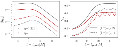
Figure 2: The amplitude (left) and mode frequency (right) evolution of the $l=2$ modes for an almost equal mass ($q=1.221$) binary (grey) and a large mass ratio ($q=10$) binary (red). Solid (dashed) lines show the $m=2$ ($m=1$) mode.

We consider two test cases from the publicly available SXS catalogue of NR simulations, SXS:BBH:0305 and SXS:BBH:1107, corresponding to non-spinning binaries with mass ratios $q=1.221$ and $q=10$, respectively. The former is a GW150914-like signal with the final mass $M_{f}=0.9520M$ and dimensionless spin $a_{f}=0.6921$. The later has a final mass $M_{f}=0.9917M$ and spin $a_{f}=0.2605$. The QNM frequencies are fixed to their GR values (and calculated using Ref. (Stein, 2019)) which leaves only the complex amplitudes as free parameters which we fit to NR using a linear least squares method. A ringdown model with overtone index upto $N$ has $2(N+1)$ complex amplitudes that are being fit. We vary the start time of ringdown from $t_{0}=t_{\rm peak}-25M$ to $t_{0}=t_{\rm peak}+50M$, where the origin $t_{0}=t_{\rm peak}$ has been taken to be the peak of the $h_{22}$ mode. We fix the end time to be $t=t_{\rm peak}+90M$ by which time even the longest lived overtone would have decayed essentially to numerical noise. We define the mismatch between the best-fit ringdown waveform ($h_{\rm fit}$) and NR waveform ($h_{\rm NR}$) by

$$\mathcal{M}=1-\frac{\langle h_{\rm NR}|h_{\rm fit}\rangle}{\sqrt{\langle h_{\rm NR}|h_{\rm NR}\rangle\langle h_{\rm fit}|h_{\rm fit}\rangle}},$$ (11)

where the inner product is defined as

$$\langle a(t)|b(t)\rangle=\int_{t_{0}}^{90M}a^{*}(t)b(t)dt.$$ (12)

We note that QNMs are not orthogonal and complete under this inner product. This has been a longstanding theoretical question and it is doubtful whether such an inner product can be defined for QNMs that is also of practical use (Nollert and Price, 1999).

In Fig. 3, we show the dependence of $\mathcal{M}$ as a function of the start time $t_{0}$. We compare $\mathcal{M}$ between our model and the reference model of Giesler et al. (2019) for up to an 8-tone ringdown waveform. The mismatch curves are qualitatively similar for both the simulations apart from the characteristic that the mismatches for the $(l,m)=(2,1)$ mode of the (almost) equal mass binary has multiple crests and troughs before hitting the numerical noise floor. We see that the mismatch for any given $t_{0}$ and ($N+1$)-tone model is lower for mirror mode model compared to the reference model. The betterment in $\mathcal{M}$ is roughly 3 orders of magnitude for an 8-tone model at $t_{0}\sim-10M$. We observe that the fundamental mirror mode is definitively excited in the $q=10$ binary and is considerable at late times as was seen in Fig. 2. We note that the mismatches for $(l,m)=(2,2)$ mode of SXS:BBH:0305 agree with Fig. 1 of Giesler et al. (2019) when mirror modes are not included, thus providing a validation for our fits.

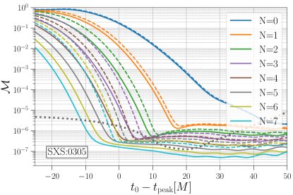
(a)

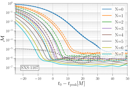
(b)

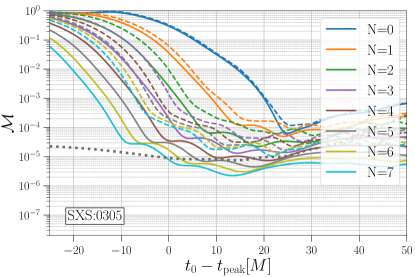
(c)

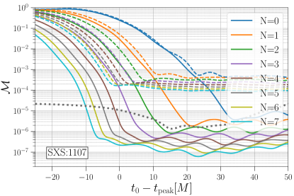
(d)

Figure 3: Comparison of mismatches $\mathcal{M}$ between mirror modes model and our reference model for an $(N+1)$-tone model for the two cases under consideration. The mismatches $\mathcal{M}$ are plotted as a function of start time $t_{0}$ whose origin is taken to be the peak of $h_{22}$. Solid (dashed) lines represent the class of ringdown models with (without) the mirror modes. The top panel shows the mismatches for $(l,m)=(2,2)$ spherical harmonic mode while the bottom panel depicts the same for $(l,m)=(2,1)$ mode. The grey, dotted, horizontal line shows the mismatch for the two highest resolution NR simulations. We note that the mismatches are always lower when the mirror modes are included with marked improvements at times before the peak of the $h_{22}$ mode.

In addition, in Fig. 3, we compute the numerical noise floor by calculating the mismatch between the waveforms of the two highest resolved NR simulations. This would give us an estimate of the truncation errors in an NR simulation due to finite grid sizes. For the modes and the cases under study, we see that the mismatch of this noise floor is between $\sim 10^{-4}$ and $\sim 10^{-7}$ with the higher mismatches occuring at late times. This is illustrated by the grey horizontal dotted lines in the figure.

The plot shows another crucial feature. An 8-tone ringdown model gives orders of magnitude lower mismatches than (say) a 2-tone model even when the ringdown is started at a late enough time ($\sim t_{\rm peak}+30M$) when all higher overtones are expected to have decayed to numerical noise. This happens at or below the numerical noise floor of the simulations used and, therefore, we believe that at these times the free parameters of the models are being fit to numerical noise and that this feature is unphysical.

We point out that even though there is a huge improvement in $\mathcal{M}$ at early times with the inclusion of mirror modes in the ringdown model, mirror modes alone do not produce good fits. The positive oscillation frequency modes are still the dominant modes (at least for the cases considered in this study) present in the waveform. It would be interesting to see if spins and precession of the progenitor binary change this conclusion.

As argued in Giesler et al. (2019), a ringdown model should not just produce a small mismatch but also recover the correct physical parameters of the system. To this end, we vary $M_{f}$ and $a_{f}$ but keep the QNM frequencies to be that determined from perturbation theory (i.e., functions of $M_{f}$ and $a_{f}$) and repeat the mismatch calculation. A ringdown signal consisting of actual BH QNMs should minimize the mismatch for the true value of $M_{f}$ and $a_{f}$ as determined from NR simulations, modulo systematic errors. A sharply peaked mismatch, on the other hand, would give better statistical errors on the remnant paramters. In Fig. 4 and Fig. 5, we plot the mismatch on a grid of $M_{f}$ and $a_{f}$ for two different start times, $t_{0}=0$ and $t_{0}=-10M$, respectively, for an 8-tone model. The left panel of each plot shows the heatmap of mismatches for the reference ringdown model and the right panel includes mirror modes in the ringdown model.

We note that when the ringdown is started at the peak of $h_{22}$ mode, the 8-tone reference model gives better estimates of the remnant parameters than a model with mirror modes for $(l,m)=(2,2)$ while for $(l,m)=(2,1)$ mode, the remnant parameter estimates are roughly the same. But if we move the ringdown start time to an earlier fiducial time $t_{0}=-10M$, our ringdown model has a deeper minimum near the correct remnant paramters. At this start time, the improvement in remnant estimates with the inclusion of mirror modes is far greater for the large mass ratio binary than the (almost) equal mass one. This, as expected, points towards a greater significance of mirror modes for large mass ratios (Berti et al., 2006). This aspect is also clear from the mismatch plots of the $(l,m)=(2,1)$ mode. The remnant parameter estimates using the $(l,m)=(2,1)$ mode is also far superior with the inclusion of mirror mode ascertaining our earlier assertion that the mirror modes excitation amplitudes depend on the value of $m$.

(a)

(b)

(c)

(d)

Figure 4: Mismatch $\mathcal{M}$ between best-fit ringdown model and NR waveform for an 8-tone model on a grid of $M_{f}-a_{f}$ for GR QNM frequencies. The start time of ringdown is taken to be $t_{0}=0$. The white crosshair denotes the true remnant mass and spin as ascertained by NR while the grey cross shows the best-fit value determined by a ringdown model. The result for the reference model is plotted on the left panel while the mirror modes model is on the right panel of each plot. The result for spherical harmonic mode $(l,m)=(2,2)$ is plotted in the top panel of the figure while the bottom panel highlights the result for the $l=2$, $m=1$ mode. The plot on the left is for the simulation SXS:0305 and the right plot is for SXS:1107.

(a)

(b)

(c)

(d)

Figure 5: Same as Fig. 4 but the ringdown start time is taken to be $t_{0}=-10M$. It is clear that a linear ringdown model including mirror modes recovers the true masses and spins much better at this time than the reference model.

In Tab. 1, we quote the value of the mismatch for the best-fit $M_{f}$ and $a_{f}$ when varied on a grid. Notice that the mirror mode model gives lower mismatches throughout with stark differences for the larger mass ratio case, $m=1$ mode, and starting time before $t_{0}=t_{\rm peak}$. The only exception is the (almost) equal mass case where minimal excitation of mirror modes are expected and, therefore, by the time of the peak of the $h_{22}$ mode, these modes are no longer significant.

We quantify the errors in the estimation of the remnant parameters using a quantity $\epsilon$, introduced in Giesler et al. (2019), defined as

$$\epsilon=\sqrt{\left(\frac{\delta M_{f}}{M}\right)^{2}+\left(\delta a_{f}\right)^{2}},$$ (13)

where $\delta M_{f}$ and $\delta a_{f}$ are the differences between the best-fit values and the true values of the remnant parameters as determined by NR. In Fig. 6 we plot $\epsilon$ as a function of the number of overtones in the ringdown model. We compare the performance of a ringdown model with mirror modes to that of the reference model. We do the comparison at two different start times, $t_{0}=t_{\rm peak}$ and $t_{0}=t_{\rm peak}-10M$. We see that when the ringdown is started at $t_{0}=t_{\rm peak}$, the mirror modes model performs as good as or even marginally better than the reference model up to a 6-tone ringdown waveform for both the spherical harmonic modes in the (almost) equal mass binary case. A higher-tone waveform model deteriorates the remnant parameter estimates for the mirror mode model. For the high mass ratio case, the situation is different with the mirror mode model performing much better than the reference model up to a 6-tone ringdown waveform for $m=2$ mode and 7-tone waveform for $m=1$ mode. If the ringdown in started at an earlier time $t_{0}=t_{\rm peak}-10M$, the mirror mode model is clearly superior to the reference model for both the spherical harmonic modes and both the mass ratios under consideration. The trend is the same for both the modes and mass ratios, with the errors in the estimation of remnant parameters decreasing monotonically with the number of included overtones and the mirror mode model performing better by a factor of $\sim 5-10$ for an 8-tone model.

	SXS:0305		SXS:1107
m	reference	mirror mode	reference	mirror mode
	$t_{0}=t_{\rm peak}$
2	$-6.51$	$-6.84$	$-6.15$	$-6.62$
1	$-3.96$	$-5.34$	$-3.79$	$-6.71$
	$t_{0}=t_{\rm peak}-10M$
2	$-3.73$	$-6.11$	$-3.88$	$-5.76$
1	$-2.94$	$-4.36$	$-2.88$	$-5.19$

Table 1: The value of the mismatch ($\log_{10}\mathcal{M}$) for the best-fit paramters in Fig. 4 and Fig. 5. Note that the mirror mode model gives orders of magnitude better mismatch for all the cases except the (almost) equal mass case starting at $t_{0}=t_{\rm peak}$ where the mismatches are similar.

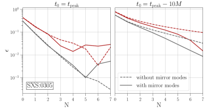
(a)

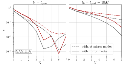
(b)

Figure 6: $\epsilon$ as a function of the number of overtones included in a ringdown model. Solid (dashed) curves are for the mirror modes (reference) model. In the left two panels, the ringdown is started at $t_{0}=t_{\rm peak}$ whereas on the right two panels, the ringdown start time is taken to be $t_{0}=t_{\rm peak}-10M$.

In Tab. 2 and Tab. 3, we quote the real-valued amplitudes of regular modes ($\mathcal{A}_{lmn}$) and mirror modes ($\mathcal{\bar{A}}_{lmn}$) for an 8-tone model for the two cases under study (SXS:0305 and SXS:1107) and the two spherical harmonic modes $(l,m)=(2,2)$ and $(l,m)=(2,1)$, respectively. The fit amplitudes are calculated at $t_{0}=-10M$. We choose a fiducial reference time $t_{0}=0$ to quote the values of the amplitudes so that they can be easily compared with the values quoted in other studies (Giesler et al., 2019; Bhagwat et al., 2020). Eventhough the mirror mode amplitudes are much larger than the regular mode amplitudes at the start time $t_{0}=-10M$, we see that the regular modes become more dominant by the time the $h_{22}$ mode peaks. At this time, the mirror modes are subdominant by close to an order of magnitude for most modes with up to $\sim 3$ orders of magnitude for $n=7$. We point out that the amplitude of the positive frequency fundamental mode calculated at $t_{0}=-10M$ and time evolved to $t_{0}=0$ is in striking agreement to that calculated at $t_{0}=0$ (and reported in Giesler et al. (2019) and Bhagwat et al. (2020)). This indicates that the positive-frequency fundamental mode has entered the linear phase even at this early time. Additionally, we observe, for both the spherical harmonic modes, that the ratio between the mirror mode amplitudes and the corresponding regular mode amplitudes ($\mathcal{\bar{A}}_{lmn}/\mathcal{A}_{lmn}$) is greater for the large mass ratio case indicating that mirror modes are more strongly excited in large mass ratio binaries. Furthermore, note that, for both the mass ratios, this ratio is larger for $(l,m)=(2,1)$ mode than $(l,m)=(2,2)$ mode, demonstrating that mirror modes are more strongly excited in $m=1$ mode than $m=2$ mode.

We note the observation in Bhagwat et al. (2020) that the best-fit amplitudes increase with the overtone number $n$, reaches a maximum around $n=3/4$ and decreases for higher $n$ holds true for the mirror mode model as well and as such provide support to their speculative reasoning that high-$n$ overtones are excited first by sources far away from the horizon and hence are weaker. By contrast, low-$n$ overtones, excited by sources closer to the horizon, falls partly into the horizon and does not reach null infinity. Consequently, intermediate-$n$ overtones are the most strongly excited.

	$(l,m)=(2,2)$
	SXS:0305		SXS:1107
n	$\mathcal{A}_{lmn}$	$\mathcal{\bar{A}}_{lmn}$	$\mathcal{A}_{lmn}$	$\mathcal{\bar{A}}_{lmn}$
0	0.972455	0.00195254	0.337405	0.00104528
1	4.04150	0.0571118	1.10677	0.0409705
2	9.93874	0.535089	3.00238	0.503610
3	17.0806	1.43902	6.14453	2.15847
4	17.7877	0.672877	6.34204	2.32482
5	8.58776	0.0602107	2.59237	0.531559
6	1.43898	0.00153011	0.347826	0.0216096
7	0.0674631	1.37488$\mathrm{e}{-05}$	0.0106518	0.000144103

Table 2: Best-fit real amplitudes of $(l,m)=(2,2)$ mode for a mirror mode model with ringdown start time $t_{0}=t_{\rm peak}-10M$. The amplitude values quoted are at $t=t_{\rm peak}$ obtained by time-evolving the respective amplitudes with their decay times. $\mathcal{A}_{lmn}$ are the amplitudes of the regular modes and $\mathcal{\bar{A}}_{lmn}$ are the mirror mode amplitudes.

	$l=2$, $m=1$
	SXS:0305		SXS:1107
n	$\mathcal{A}_{lmn}$	$\mathcal{\bar{A}}_{lmn}$	$\mathcal{A}_{lmn}$	$\mathcal{\bar{A}}_{lmn}$
0	0.0528504	0.000369536	0.125076	0.00501953
1	0.326904	0.0217794	0.746708	0.0985377
2	1.08230	0.195302	2.67917	0.873092
3	2.13312	0.566340	5.84294	3.09317
4	2.13512	0.432410	5.73515	3.29656
5	0.921344	0.0753840	2.06885	0.913868
6	0.144722	0.00289362	0.236321	0.0535978
7	0.00606425	2.65232$\mathrm{e}{-05}$	0.00624921	0.000426323

Table 3: Same as Tab. 2 but for $(l,m)=(2,1)$ mode.

Till this point, we have chosen a fiducial start time $t_{0}=t_{\rm peak}-10M$ to show the importance of mirror modes at times earlier than the peak of $h_{22}$ mode. We will now look at the effect of a varying start time for an 8-tone ringdown model. In Fig. 7, we show the error in the estimation of remnant parameters as a function of the start time. We see that for the reference model, the errors increase (virtually) monotonically the earlier the ringdown is started with respect to the peak of $h_{22}$. For a mirror mode model, the error estimates have a minima at some time between $t_{0}=t_{\rm peak}-10M$ and $t_{0}=t_{\rm peak}$ with the remnant parameter estimates using the mirror mode model being an order of magnitude more accurate. We observe that this minima occurs around the time that the mismatch curve has a minima too. Therefore, we can also use the conventional wisdom of taking the start time of ringdown at the earliest minima of a mismatch curve – which is always at an earlier time for a mirror mode model than the corresponding minima for the reference model for a sufficiently high-tone ringdown waveform – to argue the significance of mirror modes at times before the peak of $h_{22}$. Furthermore, in the case of $(l,m)=(2,2)$ mode, the minimum errors in the 8-tone mirror mode model are about the same as that for the 8-tone reference model started at $t_{0}=t_{\rm peak}$ but with the advantage that the mirror mode model achieves this at a much earlier time, thereby accumulating more energy in the ringdown signal. The situation is even better for $(l,m)=(2,1)$ mode where not only do the minimum errors occur far before the peak of $h_{22}$ mode but also the errors are much smaller than that achieved by the reference model started at $t_{0}=t_{\rm peak}$.

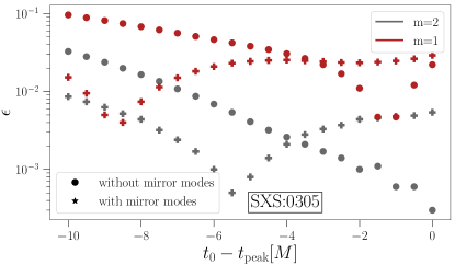
(a)

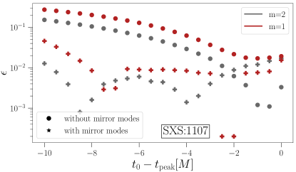
(b)

Figure 7: $\epsilon$ as a function of the start time of ringdown $t_{0}$ for an 8-tone model. Filled circles (pluses) show the value for reference (mirror mode) model. Note that $\epsilon$ is consistently lower for the mirror mode model at early times for both the spherical harmonic modes.

We provide a speculative reasoning for why the remnant parameter estimates are better in the absence of mirror modes when the ringdown is started near the peak of $h_{22}$ mode. We reason this to be because mirror modes start well before the peak of $h_{22}$ – we have seen that the fundamental positive frequency mode has already entered the ringdown phase at $-10M$ – and due to their weaker excitation and shorter damping times compared to regular modes (especially for the higher overtones where the difference in damping times becomes large), they decay to numerical noise by the time the $h_{22}$ mode peaks. This line of reasoning has support from Fig. 6 where one sees that the inclusion of mirror modes improves parameter estimation for lower-tone models mainly for the large mass ratio case where these negative-oscillation frequencies are excited more strongly. In principle, different modes should start at different times but allowing for this in a pure ringdown model would introduce unphysical discontinuities in the waveform or waveform derivatives (see Bhagwat et al. (2020) for an expanded discussion). An option would be to attach higher order perturbation theory waveforms to modes that start later so as to have a common earlier starting time for a higher order ringdown waveform but that is beyond the scope of the current work.

IV Conclusion and Discussion

In this work, we studied the effects of including negative oscillation frequency modes in a ringdown waveform which we call ‘mirror’ modes. A ringdown signal from a non-spinning BBH merger has no apriori reason to consist of only corotating modes and, therefore, mirror modes should be included in the ringdown waveform for a more accurate description of the gravitational wave signal. We find that including mirror modes decreases the mismatch of our best-fit model with NR waveforms, with up to $\sim 3$ orders of magnitude improvement at times well before the peak of the $h_{22}$ mode. We further check whether the mismatches are minimized for the true values of mass and spin, if they are allowed to vary, and find that the mirror mode model determines the remnant parameters better if the ringdown is started $6-9M$ before the peak of the $h_{22}$ mode. On the other hand, an 8-tone ringdown model with only corotating modes gives better estimates of the remnant paramters if the ringdown is started at the peak of $h_{22}$ for the $(l,m)=(2,2)$ mode because mirror modes are not excited strongly for the $m=2$ mode, although a 6-tone mirror mode model performs as good as a 6-tone reference model for the almost equal mass binary and an 8-tone reference model for the large mass ratio binary. We reason that the poorer performance of the mirror mode model when starting the ringdown at $t_{0}=t_{\rm peak}$ is because the mirror modes are excited at earlier times and they decay to numerical noise by the the time of the peak of $h_{22}$ mode. We note that more work needs to be done in this regard to verify this claim. Having different start times for each mode would lead to unphysical discontinuities in the waveform or its derivatives and, therefore, presents a technical challenge in pure ringdown modeling. A possible route is to include second-order contributions and start the ringdown at an earlier time. This would ensure smooth transition to linear regime for all the modes.

A source of systematic that can affect our results is the use of mismatch as a quantifier for our fits. It has been argued by Nollert (1999) and later by Berti et al. (2007) that the fit-amplitudes of a mismatch-based approach cannot be regarded as the physical modes excited in the system. A better quantifier is Nollert’s energy maximized orthogonal projection (EMOP) that gives the energy parallel to a given QNM (Nollert, 1999; Berti et al., 2007). We also point out that $\mathcal{M}$ as a function of the remnant parameters ($M_{f}$ and $a_{f}$) is an oscillatory function with multiple local crests and troughs, which is an undesirable feature, not least because of the difficulty of locating the true remnant values.

If we trust the ringdown fits as the QNMs excited in the system, then it poses the question of what happened to all the non-linearities present in the system? Bhagwat et al. (2020) argue that the conclusions of recent works to model the post-merger signal with a pure ringdown model is at odds with Bhagwat et al. (2018), where the authors find appreciable non-linearities in the source frame near the common horizon. We bring to notice a more recent work of Okounkova (2020) that uses the same quantifiers of non-linearity as that used in Bhagwat et al. (2018). The author then time evolves the gauge invariant quantifiers and finds that the non-linearities fall into the common horizon soon after its formation and does not reach asymptotic infinity.

We believe further progress in ringdown modeling should take into account these findings. Future work will include feasibility studies of detecting these mirror modes in LISA signals and in third generation ground-based detectors. We are also in the process of using this model to recover the remnant parameters for select events published by LIGO/Virgo.