Nonrelativistic one-particle problem on $q$-deformed Euclidean space

Abstract

We consider time-dependent Schrödinger equations for a free nonrelativistic particle on the three-dimensional $q$-deformed Euclidean space. We determine plane wave solutions to these Schrödinger equations and show that they form a complete orthonormal system. We derive $q$-deformed expressions for propagators of a nonrelativistic particle. Considerations about expectation values for position or momentum of a nonrelativistic particle conclude our studies.

1 Introduction

Describing space-time as a continuum is a very successful concept in physics. Various considerations, however, suggest that the Planck length limits the accuracy of spatial measurements [1, 2]. This uncertainty in space-time suggests that describing space-time as a continuum is no longer appropriate for small space-time distances.

In quantum mechanics, Heisenberg’s commutation relations for position coordinates and momentum coordinates imply that the state of a particle in phase space is not accurately determined. We can assume analogously that the uncertainty in position measurements is due to a noncommutativity of position operators:

$$[\hskip 0.72229pt\hat{x}^{i},\hat{x}^{j}]=\theta^{ij}(\hat{x}).$$ (1)

H. Snyder was one of the first who tried to construct a quantized space-time with non-commuting position coordinates [3]. In recent times the focus has been on noncommutative space-time algebras with $\theta^{ij}\in\mathbb{C}$ [4, 5, 6, 7]. Furthermore, space-time algebras with the commutator in Eq. (1) being a linear function of space-time coordinates, i. e. $\theta^{ij}(\hat{x})=\Theta_{k}^{ij}\hskip 0.72229pt\hat{x}^{k}$, are also of particular interest [8, 9]. We consider, however, the $q$-deformed Euclidean space [10], which is a noncommutative space with quadratic relations, i. e. $\theta^{ij}(\hat{x})=\Theta_{kl}^{ij}\hskip 0.72229pt\hat{x}^{k}\hat{x}^{l}$.

The commutation relations for the coordinates of $q$-deformed Euclidean space satisfy the Poincaré-Birkhoff-Witt property. It says that each vector space generated by homogeneous polynomials with a fixed degree has the same dimension as in the commutative case with $\theta^{ij}(\hat{x})=0$. Thus the normal-ordered monomials of noncommutative coordinates form a basis of $q$-deformed Euclidean space. For this reason, we can associate the noncommutative algebra of $q$-deformed Euclidean space with a commutative coordinate algebra by using the star-product formalism [11].

The star-product formalism enables us to construct a $q$-deformed version of mathematical analysis [12, 13]. In Ref. [14], we have discussed $q$-deformed momentum eigenfunctions within the framework of this $q$-deformed analysis. We have shown in Ref. [15] that the time evolution operator of a quantum system in $q$-deformed Euclidean space is of the same form as in the undeformed case. In this article, we are going to apply our findings to a nonrelativistic particle in $q$-deformed Euclidean space.

First, we give $q$-analogs for the Hamilton operator of a free, nonrelativistic particle. Next, we construct $q$-deformed plane wave solutions to the corresponding Schrödinger equations. We also show that the $q$-deformed plane waves form a complete orthonormal set of functions. This fact enables us to write down $q$-deformed versions of the propagator for a nonrelativistic particle. Finally, we show how to calculate expectation values of position or momentum with the solutions of our $q$-deformed Schrödinger equations.

2 Preliminaries

2.1 Star-products

The three-dimensional $q$-deformed Euclidean space $\mathbb{R}_{q}^{3}$ has the generators $X^{+}$, $X^{3}$, and $X^{-}$, subject to the following commutation relations [16]:

$$X^{3}X^{+} =q^{2}X^{+}X^{3},$$

$$X^{3}X^{-} =q^{-2}X^{-}X^{3},$$

$$X^{-}X^{+} =X^{+}X^{-}+(q-q^{-1})\hskip 0.72229ptX^{3}X^{3}.$$ (2)

We can extend the algebra of $\mathbb{R}_{q}^{3}$ by a time element $X^{0}$, which commutes with the generators $X^{+}$, $X^{3}$, and $X^{-}$ [15]:

$$X^{0}X^{A}=X^{A}X^{0},\text{\qquad}A\in\{+,3,-\}.$$ (3)

In the following, we refer to the algebra spanned by the generators $X^{i}$ with $i\in\{0,+,3,-\}$ as $\mathbb{R}_{q}^{3,t}$.

There is a $q$-analog of the three-dimensional Euclidean metric $g^{AB}$ with its inverse $g_{AB}$ [16] (rows and columns are arranged in the order $+,3,-$):

$$g_{AB}=g^{AB}=\left(\begin{array}[c]{ccc}0&0&-\hskip 0.72229ptq\\ 0&1&0\\ -\hskip 0.72229ptq^{-1}&0&0\end{array}\right).$$ (4)

We can use the $q$-deformed metric to raise and lower indices:

$$X_{A}=g_{AB}\hskip 0.72229ptX^{B},\qquad X^{A}=g^{AB}X_{B}.$$ (5)

The algebra $\mathbb{R}_{q}^{3,t}$ has a semilinear, involutive, and anti-multiplicative mapping, which we call quantum space conjugation. If we indicate conjugate elements of a quantum space by a bar, we can write the properties of quantum space conjugation as follows ($\alpha,\beta\in\mathbb{C}$ and $u,v\in\mathbb{R}_{q}^{3,t}$):

$$\overline{\alpha\,u+\beta\,v}=\overline{\alpha}\,\overline{u}+\overline{\beta}\,\overline{v},\quad\overline{\overline{u}}=u,\quad\overline{u\,v}=\overline{v}\,\overline{u}.$$ (6)

The conjugation for $\mathbb{R}_{q}^{3,t}$ is compatible with the commutation relations in Eq. (2) and Eq. (3) if the following applies [15]:

$$\overline{X^{A}}=X_{A}=g_{AB}\hskip 0.72229ptX^{B},\qquad\overline{X^{0}}=X_{0}.$$ (7)

We can only prove a physical theory if it predicts measurement results. The problem, however, is: How can we associate the elements of the noncommutative space $\mathbb{R}_{q}^{3,t}$ with real numbers? One solution to this problem is to introduce a vector space isomorphism between the noncommutative algebra $\mathbb{R}_{q}^{3,t}$ and a corresponding commutative coordinate algebra $\mathbb{C}[\hskip 0.72229ptx^{+},x^{3},x^{-},t\hskip 0.72229pt]$.

We recall that the normal-ordered monomials in the generators $X^{i}$ form a basis of the algebra $\mathbb{R}_{q}^{3,t}$, i. e. we can write each element $F\in$ $\mathbb{R}_{q}^{3,t}$ uniquely as a finite or infinite linear combination of monomials with a given normal ordering (Poincaré-Birkhoff-Witt property):

$$F=\sum\limits_{n_{+},\ldots,\hskip 0.72229ptn_{0}}a_{\hskip 0.72229ptn_{+}\ldots\hskip 0.72229ptn_{0}}\,(X^{+})^{n_{+}}(X^{3})^{n_{3}}(X^{-})^{n_{-}}(X^{0})^{n_{0}},\quad\quad a_{\hskip 0.72229ptn_{+}\ldots\hskip 0.72229ptn_{0}}\in\mathbb{C}.$$ (8)

Since the monomials $(x^{+})^{n_{+}}(x^{3})^{n_{3}}(x^{-})^{n_{-}}t^{\hskip 0.72229ptn_{0}}$ with $n_{+},\ldots,n_{0}\in\mathbb{N}_{0}$ form a basis of the commutative algebra $\mathbb{C}[\hskip 0.72229ptx^{+},x^{3},x^{-},t\hskip 0.72229pt]$, we can define a vector space isomorphism

$$\mathcal{W}:\mathbb{C}[\hskip 0.72229ptx^{+},x^{3},x^{-},t\hskip 0.72229pt]\rightarrow\mathbb{R}_{q}^{3,t}$$ (9)

with

$$\mathcal{W}\left((x^{+})^{n_{+}}(x^{3})^{n_{3}}(x^{-})^{n_{-}}t^{\hskip 0.72229ptn_{0}}\right)=(X^{+})^{n_{+}}(X^{3})^{n_{3}}(X^{-})^{n_{-}}(X^{0})^{n_{0}}.$$ (10)

In general, we have

$$\mathbb{C}[\hskip 0.72229ptx^{+},x^{3},x^{-},t\hskip 0.72229pt]\ni f\mapsto F\in\mathbb{R}_{q}^{3,t},$$ (11)

where

$$f =\sum\limits_{n_{+},\ldots,\hskip 0.72229ptn_{0}}a_{\hskip 0.72229ptn_{+}\ldots\hskip 0.72229ptn_{0}}\,(x^{+})^{n_{+}}(x^{3})^{n_{3}}(x^{-})^{n_{-}}t^{\hskip 0.72229ptn_{0}},$$

$$F =\sum\limits_{n_{+},\ldots,\hskip 0.72229ptn_{0}}a_{\hskip 0.72229ptn_{+}\ldots\hskip 0.72229ptn_{0}}\,(X^{+})^{n_{+}}(X^{3})^{n_{3}}(X^{-})^{n_{-}}(X^{0})^{n_{0}}.$$ (12)

The vector space isomorphism $\mathcal{W}$ is nothing else but the Moyal-Weyl mapping, which gives an operator $F$ to a complex valued function $f$ [17, 18, 19, 11].

We can extend this vector space isomorphism to an algebra isomorphism if we introduce a new product on the commutative coordinate algebra. This so-called star-product symbolized by $\circledast$ satisfies the following homomorphism condition:

$$\mathcal{W}\left(f\circledast g\right)=\mathcal{W}\left(f\right)\cdot\mathcal{W}\left(\hskip 0.72229ptg\right).$$ (13)

Since the Moyal-Weyl mapping is invertible, we can write the star-product as follows:

$$f\circledast g=\mathcal{W}^{\hskip 0.72229pt-1}\big{(}\,\mathcal{W}\left(f\right)\cdot\mathcal{W}\left(\hskip 0.72229ptg\right)\big{)}.$$ (14)

To get explicit formulas for calculating star-products, we first have to write a noncommutative product of two normal-ordered monomials as a linear combination of normal-ordered monomials again (see Ref. [20] for details):

$$(X^{+})^{n_{+}}\ldots\hskip 0.72229pt(X^{0})^{n_{0}}\cdot(X^{+})^{m_{+}}\ldots\hskip 0.72229pt(X^{0})^{m_{0}}=\sum_{\underline{k}\hskip 0.72229pt=\hskip 0.72229pt0}B_{\underline{k}}^{\hskip 0.72229pt\underline{n},\underline{m}}\,(X^{+})^{k_{+}}\ldots\hskip 0.72229pt(X^{0})^{k_{0}}.$$ (15)

We achieve this by using the commutation relations for the noncommutative coordinates [cf. Eq. (2)]. From the concrete form of the series expansion in Eq. (15), we can finally read off a formula to calculate the star-product of two power series in commutative space-time coordinates ($\lambda=q-q^{-1}$): 

$$f(\mathbf{x},t)\circledast g(\mathbf{x},t)=$$

$$\sum_{k\hskip 0.72229pt=\hskip 0.72229pt0}^{\infty}\lambda^{k}\hskip 0.72229pt\frac{(x^{3})^{2k}}{[[k]]_{q^{4}}!}\,q^{2(\hat{n}_{3}\hskip 0.72229pt\hat{n}_{+}^{\prime}+\,\hat{n}_{-}\hat{n}_{3}^{\prime})}D_{q^{4},\hskip 0.72229ptx^{-}}^{k}f(\mathbf{x},t)\,D_{q^{4},\hskip 0.72229ptx^{\prime+}}^{k}g(\mathbf{x}^{\prime},t)\big{|}_{x^{\prime}\rightarrow\hskip 0.72229ptx}.$$ (16)

The argument $\mathbf{x}$ indicates a dependence on the spatial coordinates $x^{+}$, $x^{3}$, and $x^{-}$. Note that the expression above depends on the operators

$$\hat{n}_{A}=x^{A}\frac{\partial}{\partial x^{A}}$$ (17)

and the so-called Jackson derivatives [21]:

$$D_{q^{k},\hskip 0.72229ptx}\,f=\frac{f(q^{k}x)-f(x)}{q^{k}x-x}.$$ (18)

Moreover, the $q$-numbers are given by

$$[[a]]_{q}=\frac{1-q^{a}}{1-q},$$ (19)

and the $q$-factorials are defined in complete analogy to the undeformed case:

$$[[\hskip 0.72229ptn]]_{q}!=[[1]]_{q}\hskip 0.72229pt[[2]]_{q}\ldots[[\hskip 0.72229ptn-1]]_{q}\hskip 0.72229pt[[\hskip 0.72229ptn]]_{q},\qquad[[0]]_{q}!=1.$$ (20)

The algebra isomorphism $\mathcal{W}^{-1}$ also enables us to carry over the conjugation for the quantum space algebra $\mathbb{R}_{q}^{3,t}$ to the commutative coordinate algebra $\mathbb{C}[\hskip 0.72229ptx^{+},x^{3},x^{-},t\hskip 0.72229pt]$. In other words, the mapping $\mathcal{W}^{\hskip 0.72229pt-1}$ is a $\ast$-algebra homomorphism:

$$\mathcal{W}(\hskip 0.72229pt\overline{f}\hskip 0.72229pt)=\overline{\mathcal{W}(f)}\qquad\Leftrightarrow\text{\qquad}\overline{f}=\mathcal{W}^{-1}\big{(}\hskip 0.72229pt\overline{\mathcal{W}(f)}\hskip 0.72229pt\big{)}.$$ (21)

This relationship implies the following property for the star-product:

$$\overline{f\circledast g}=\overline{g}\circledast\overline{f}.$$ (22)

With $\bar{f}$, we designate the power series obtained from $f$ by quantum space conjugation. If $\bar{a}_{n_{+},n_{3},n_{-},n_{0}}$ stands for the complex conjugate of $a_{n_{+},n_{3},n_{-},n_{0}}$, Eqs. (7) and (21) yield that $\bar{f}$ takes the following form [13, 15]:

$$\overline{f(\mathbf{x},t)} =\sum\nolimits_{\underline{n}}\bar{a}_{\hskip 0.72229ptn_{+},n_{3},n_{-},n_{0}}\,(-\hskip 0.72229ptq\hskip 0.72229ptx^{-})^{n_{+}}(\hskip 0.72229ptx^{3})^{n_{3}}(-\hskip 0.72229ptq^{-1}x^{+})^{n_{-}}t^{n_{0}}$$

$$=\sum\nolimits_{\underline{n}}(-\hskip 0.72229ptq)^{n_{-}-\hskip 0.72229ptn_{+}}\hskip 0.72229pt\bar{a}_{\hskip 0.72229ptn_{-},n_{3},n_{+},n_{0}}\,(\hskip 0.72229ptx^{+})^{n_{+}}(\hskip 0.72229ptx^{3})^{n_{3}}(\hskip 0.72229ptx^{-})^{n_{-}}t^{n_{0}}$$

$$=\bar{f}(\mathbf{x},t).$$ (23)

2.2 Partial derivatives and integrals

There are partial derivatives for $q$-deformed space-time coordinates [22, 23]. These partial derivatives again form a quantum space with the same algebraic structure as that of the $q$-deformed space-time coordinates. Thus, the $q$-deformed partial derivatives $\partial_{i}$ satisfy the same commutation relations as the covariant coordinate generators $X_{i}$:

$$\partial_{0}\hskip 0.72229pt\partial_{+}=\hskip 0.72229pt\partial_{+}\hskip 0.72229pt\partial_{0},\quad\partial_{0}\hskip 0.72229pt\partial_{-}=\hskip 0.72229pt\partial_{-}\hskip 0.72229pt\partial_{0},\quad\partial_{0}\hskip 0.72229pt\partial_{3}=\partial_{3}\hskip 0.72229pt\partial_{0},$$

$$\partial_{+}\hskip 0.72229pt\partial_{3}=q^{2}\partial_{3}\hskip 0.72229pt\partial_{+},\quad\partial_{3}\hskip 0.72229pt\partial_{-}=\hskip 0.72229ptq^{2}\partial_{-}\hskip 0.72229pt\partial_{3},$$

$$\partial_{+}\hskip 0.72229pt\partial_{-}-\partial_{-}\hskip 0.72229pt\partial_{+}=\hskip 0.72229pt\lambda\hskip 0.72229pt\partial_{3}\hskip 0.72229pt\partial_{3}.$$ (24)

The commutation relations above are invariant under conjugation if the derivatives show the following conjugation properties:

$$\overline{\partial_{A}}=-\hskip 0.72229pt\partial^{A}=-g^{AB}\partial_{B},\qquad\overline{\partial_{0}}=-\hskip 0.72229pt\partial^{0}=-\hskip 0.72229pt\partial_{0}.$$ (25)

There are two ways of commuting $q$-deformed partial derivatives with $q$-deformed space-time coordinates. One is given by the following $q$-deformed Leibniz rules [22, 23, 15]:

$$\partial_{B}X^{A} =\delta_{B}^{A}+q^{4}\hat{R}{{}^{AC}}_{BD}\,X^{D}\partial_{C},$$

$$\partial_{A}X^{0} =X^{0}\hskip 0.72229pt\partial_{A},$$

$$\partial_{0}\hskip 0.72229ptX^{A} =X^{A}\hskip 0.72229pt\partial_{0},$$

$$\partial_{0}\hskip 0.72229ptX^{0} =1+X^{0}\hskip 0.72229pt\partial_{0}.$$ (26)

Note that $\hat{R}{{}^{AC}}_{BD}$ denotes the vector representation of the R-matrix for the three-dimensional $q$-deformed Euclidean space.

By conjugation, we can obtain the Leibniz rules for another differential calculus from the identities in Eq. (26). Introducing $\hat{\partial}_{A}=q^{6}\partial_{A}$ and $\hat{\partial}_{0}=\partial_{0}$, we can write the Leibniz rules of this second differential calculus in the following form:

$$\hat{\partial}_{B}\hskip 0.72229ptX^{A} =\delta_{B}^{A}+q^{-4}(\hat{R}^{-1}){{}^{AC}}_{BD}\,X^{D}\hat{\partial}_{C},$$

$$\hat{\partial}_{A}\hskip 0.72229ptX^{0} =X^{0}\hskip 0.72229pt\hat{\partial}_{A},$$

$$\hat{\partial}_{0}\hskip 0.72229ptX^{A} =X^{A}\hskip 0.72229pt\hat{\partial}_{0},$$

$$\hat{\partial}_{0}\hskip 0.72229ptX^{0} =1+X^{0}\hskip 0.72229pt\hat{\partial}_{0}.$$ (27)

Using the Leibniz rules in Eq. (26) or Eq. (27), we can calculate how partial derivatives act on normal-ordered monomials of noncommutative coordinates. We can carry over these actions to commutative coordinate monomials with the help of the Moyal-Weyl mapping:

$$\partial^{i}\triangleright(x^{+})^{n_{+}}(x^{3})^{n_{3}}(x^{-})^{n_{-}}t^{\hskip 0.72229ptn_{0}}=\mathcal{W}^{\hskip 0.72229pt-1}\big{(}\partial^{i}\triangleright(X^{+})^{n_{+}}(X^{3})^{n_{3}}(X^{-})^{n_{-}}(X^{0})^{n_{0}}\big{)}.$$ (28)

Since the Moyal-Weyl mapping is linear, we can apply the action above to space-time functions that can be written as a power series:

$$\partial^{i}\triangleright f(\mathbf{x},t)=\mathcal{W}^{\hskip 0.72229pt-1}\big{(}\partial^{i}\triangleright\mathcal{W}(f(\mathbf{x},t))\big{)}.$$ (29)

If we use the ordering given in Eq. (10) of the previous chapter, the Leibniz rules in Eq. (26) lead to the following operator representations [24]:

$$\partial_{+}\triangleright f(\mathbf{x},t) =D_{q^{4},\hskip 0.72229ptx^{+}}f(\mathbf{x},t),$$

$$\partial_{3}\triangleright f(\mathbf{x},t) =D_{q^{2},\hskip 0.72229ptx^{3}}f(q^{2}x^{+},x^{3},x^{-},t),$$

$$\partial_{-}\triangleright f(\mathbf{x},t) =D_{q^{4},\hskip 0.72229ptx^{-}}f(x^{+},q^{2}x^{3},x^{-},t)+\lambda\hskip 0.72229ptx^{+}D_{q^{2},\hskip 0.72229ptx^{3}}^{2}f(\mathbf{x},t).$$ (30)

The derivative $\partial_{0}$, however, is represented on the commutative space-time algebra by an ordinary partial derivative:

$$\partial_{0}\triangleright f(\mathbf{x},t)=\frac{\partial f(\mathbf{x},t)}{\partial t}.$$ (31)

Using the Leibniz rules in Eq. (27), we get operator representations for the partial derivatives $\hat{\partial}_{i}$. The Leibniz rules in Eq. (26) and Eq. (27) are transformed into each other by the following substitutions:

$$q\rightarrow q^{-1},\quad X^{-}\rightarrow X^{+},\quad X^{+}\rightarrow X^{-},$$

$$\partial^{\hskip 0.72229pt+}\rightarrow\hat{\partial}^{\hskip 0.72229pt-},\quad\partial^{\hskip 0.72229pt-}\rightarrow\hat{\partial}^{\hskip 0.72229pt+},\quad\partial^{\hskip 0.72229pt3}\rightarrow\hat{\partial}^{\hskip 0.72229pt3},\quad\partial^{\hskip 0.72229pt0}\rightarrow\hat{\partial}^{\hskip 0.72229pt0}.$$ (32)

For this reason, we obtain the operator representations of the partial derivatives $\hat{\partial}_{A}$ from those of the partial derivatives $\partial_{A}$ [cf. Eq. (30)] if we replace $q$ by $q^{-1}$ and exchange the indices $+$ and $-$:

$$\hat{\partial}_{-}\,\bar{\triangleright}\,f(\mathbf{x},t) =D_{q^{-4},\hskip 0.72229ptx^{-}}f(\mathbf{x},t),$$

$$\hat{\partial}_{3}\,\bar{\triangleright}\,f(\mathbf{x},t) =D_{q^{-2},\hskip 0.72229ptx^{3}}f(q^{-2}x^{-},x^{3},x^{+},t),$$

$$\hat{\partial}_{+}\,\bar{\triangleright}\,f(\mathbf{x},t) =D_{q^{-4},\hskip 0.72229ptx^{+}}f(x^{-},q^{-2}x^{3},x^{+},t)-\lambda\hskip 0.72229ptx^{-}D_{q^{-2},\hskip 0.72229ptx^{3}}^{2}f(\mathbf{x},t).$$ (33)

Once again, $\hat{\partial}_{0}$ is represented on the commutative space-time algebra by an ordinary partial derivative:

$$\hat{\partial}_{0}\,\bar{\triangleright}\,f(\mathbf{x},t)=\frac{\partial f(\mathbf{x},t)}{\partial t}.$$ (34)

Due to the substitutions given in Eq. (32), the actions in Eqs. (33) and (34) refer to normal-ordered monomials different from those in Eq. (10) of the previous chapter:

$$\widetilde{\mathcal{W}}\left(t^{\hskip 0.72229ptn_{0}}(x^{+})^{n_{+}}(x^{3})^{n_{3}}(x^{-})^{n_{-}}\right)=(X^{0})^{n_{0}}(X^{-})^{n_{-}}(X^{3})^{n_{3}}(X^{+})^{n_{+}}.$$ (35)

We should not forget that we can also commute $q$-deformed partial derivatives from the right side of a normal-ordered monomial to the left side by using the Leibniz rules. This way, we get the so-called right-representations of partial derivatives, for which we write $f\,\bar{\triangleleft}\,\partial^{i}$ or $f\triangleleft\hat{\partial}^{i}$. Note that the operation of conjugation transforms left actions of partial derivatives into right actions and vice versa [24]:

$$\overline{\partial^{i}\triangleright f} =-\bar{f}\,\bar{\triangleleft}\,\partial_{i}, \overline{f\,\bar{\triangleleft}\,\partial^{i}} =-\hskip 0.72229pt\partial_{i}\triangleright\bar{f},$$

$$\overline{\hat{\partial}^{i}\,\bar{\triangleright}\,f} =-\bar{f}\triangleleft\hat{\partial}_{i}, \overline{f\triangleleft\hat{\partial}^{i}} =-\hskip 0.72229pt\hat{\partial}_{i}\,\bar{\triangleright}\,\bar{f}.$$ (36)

In general, the operator representations in Eqs. (30) and (33) consist of two terms, which we call $\partial_{\operatorname*{cla}}^{A}$ and $\partial_{\operatorname*{cor}}^{A}$:

$$\partial^{A}\triangleright F=\left(\partial_{\operatorname*{cla}}^{A}+\partial_{\operatorname*{cor}}^{A}\right)\triangleright F.$$ (37)

In the undeformed limit $q\rightarrow 1$, $\partial_{\operatorname*{cla}}^{A}$ becomes an ordinary partial derivative, and $\partial_{\operatorname*{cor}}^{A}$ disappears. We get a solution to the difference equation $\partial^{A}\triangleright F=f$ with given $f$ by using the following formula [25]:

$$F =(\partial^{A})^{-1}\triangleright f=\left(\partial_{\operatorname*{cla}}^{A}+\partial_{\operatorname*{cor}}^{A}\right)^{-1}\triangleright f$$

$$=\sum_{k\hskip 0.72229pt=\hskip 0.72229pt0}^{\infty}\left[-(\partial_{\operatorname*{cla}}^{A})^{-1}\partial_{\operatorname*{cor}}^{A}\right]^{k}(\partial_{\operatorname*{cla}}^{A})^{-1}\triangleright f.$$ (38)

Applying the above formula to the operator representations in Eq. (30), we get

$$(\partial_{+})^{-1}\triangleright f(\mathbf{x},t) =D_{q^{4},\hskip 0.72229ptx^{+}}^{-1}f(\mathbf{x},t),$$

$$(\partial_{3})^{-1}\triangleright f(\mathbf{x},t) =D_{q^{2},\hskip 0.72229ptx^{3}}^{-1}f(q^{-2}x^{+},x^{3},x^{-},t),$$ (39)

and

$$(\partial_{-})^{-1}\triangleright f(\mathbf{x},t)=$$

$$=\sum_{k\hskip 0.72229pt=\hskip 0.72229pt0}^{\infty}q^{2k\left(k\hskip 0.72229pt+1\right)}\left(-\lambda\,x^{+}D_{q^{4},\hskip 0.72229ptx^{-}}^{-1}D_{q^{2},\hskip 0.72229ptx^{3}}^{2}\right)^{k}D_{q^{4},\hskip 0.72229ptx^{-}}^{-1}f(x^{+},q^{-2\left(k\hskip 0.72229pt+1\right)}x^{3},x^{-},t).$$ (40)

Note that $D_{q,\hskip 0.72229ptx}^{-1}$ stands for a Jackson integral with $x$ being the variable of integration [26]. The explicit form of this Jackson integral depends on its limits of integration and the value for the deformation parameter $q$. If $x>0$ and $q>1$, for example, the following applies:

$$\int_{0}^{\hskip 0.72229ptx}\text{d}_{q}z\hskip 0.72229ptf(z)=(q-1)\hskip 0.72229ptx\sum_{j=1}^{\infty}q^{-j}f(q^{-j}x).$$ (41)

Finally, the integral for the time coordinate is an ordinary integral since $\partial_{0}$ acts on the commutative space-time algebra like an ordinary partial derivative [cf. Eq. (31)]:

$$(\partial_{0})^{-1}\triangleright f(\mathbf{x},t)\hskip 0.72229pt=\int\text{d}t\,f(\mathbf{x},t).$$ (42)

The above considerations also apply to the partial derivatives with a hat. However, we can obtain the representations of $\hat{\partial}_{i}$ from those of the derivatives $\partial_{i}$ if we replace $q$ with $q^{-1}$ and exchange the indices $+$ and $-$. Applying these substitutions to the expressions in Eqs. (39) and (40), we immediately get the corresponding results for the partial derivatives $\hat{\partial}_{i}$.

By successively applying the integral operators given in Eqs. (39) and (40), we can explain an integration over all space [25, 13]:

$$\int_{-\infty}^{+\infty}\text{d}_{q}^{3}x\,f(x^{+},x^{3},x^{-})=(\partial_{-})^{-1}\big{|}_{-\infty}^{+\infty}\,(\partial_{3})^{-1}\big{|}_{-\infty}^{+\infty}\,(\partial_{+})^{-1}\big{|}_{-\infty}^{+\infty}\triangleright f.$$ (43)

On the right-hand side of the above relation,the different integral operators can be simplified to Jackson integrals [25, 27]:

$$\int_{-\infty}^{+\infty}\text{d}_{q}^{3}x\,f(\mathbf{x})=D_{q^{2},\hskip 0.72229ptx^{-}}^{-1}\big{|}_{-\infty}^{+\infty}\,D_{q,x^{3}}^{-1}\big{|}_{-\infty}^{+\infty}\,D_{q^{2},\hskip 0.72229ptx^{+}}^{-1}\big{|}_{-\infty}^{+\infty}\,f(\mathbf{x}).$$ (44)

Note that the Jackson integrals in the formula above refer to a smaller $q$-lattice. Using such a smaller $q$-lattice ensures that our integral over all space is a scalar with trivial braiding properties [28].

The $q$-integral over all space shows some significant features [13, 27]. In this respect, $q$-deformed versions of Stokes’ theorem apply:

$$\int_{-\infty}^{+\infty}\text{d}_{q}^{3}x\,\partial^{A}\triangleright f =\int_{-\infty}^{+\infty}\text{d}_{q}^{3}x\,f\,\bar{\triangleleft}\,\partial^{A}=0,$$

$$\int_{-\infty}^{+\infty}\text{d}_{q}^{3}x\,\hat{\partial}^{A}\,\bar{\triangleright}\,f =\int_{-\infty}^{+\infty}\text{d}_{q}^{3}x\,f\triangleleft\hat{\partial}^{A}=0.$$ (45)

The $q$-deformed Stokes’ theorem also implies rules for integration by parts:

$$\int_{-\infty}^{+\infty}\text{d}_{q}^{3}x\,f\circledast(\partial^{A}\triangleright g) =\int_{-\infty}^{+\infty}\text{d}_{q}^{3}x\,(f\triangleleft\partial^{A})\circledast g,$$

$$\int_{-\infty}^{+\infty}\text{d}_{q}^{3}x\,f\circledast(\hat{\partial}^{A}\,\bar{\triangleright}\,g) =\int_{-\infty}^{+\infty}\text{d}_{q}^{3}x\,(f\,\bar{\triangleleft}\,\hat{\partial}^{A})\circledast g.$$ (46)

Finally, we mention that the $q$-integral over all space behaves as follows under quantum space conjugation:

$$\overline{\int_{-\infty}^{+\infty}\text{d}_{q}^{3}x\,f}=\int_{-\infty}^{+\infty}\text{d}_{q}^{3}x\,\bar{f}.$$ (47)

2.3 Exponentials and Translations

A $q$-deformed exponential is an eigenfunction of each partial derivative of a given $q$-deformed quantum space [29, 30, 31]. In the following, we consider $q$-deformed exponentials that are eigenfunctions for left actions or right actions of partial derivatives:

$$\text{i}^{-1}\partial^{A}\triangleright\exp_{q}(\mathbf{x}|\text{i}\mathbf{p}) =\exp_{q}(\mathbf{x}|\text{i}\mathbf{p})\circledast p^{A},$$

$$\exp_{q}(\text{i}^{-1}\mathbf{p}|\hskip 0.72229pt\mathbf{x})\,\bar{\triangleleft}\,\partial^{A}\text{i}^{-1} =p^{A}\circledast\exp_{q}(\text{i}^{-1}\mathbf{p}|\hskip 0.72229pt\mathbf{x}).$$ (48)

The above eigenvalue equations are shown graphically in Fig. 1. The $q$-exponentials are uniquely defined by their eigenvalue equations and the following normalization conditions:

$$\exp_{q}(\mathbf{x}|\text{i}\mathbf{p})|_{x\hskip 0.72229pt=\hskip 0.72229pt0} =\exp_{q}(\mathbf{x}|\text{i}\mathbf{p})|_{p\hskip 0.72229pt=\hskip 0.72229pt0}=1,$$

$$\exp_{q}(\text{i}^{-1}\mathbf{p}|\hskip 0.72229pt\mathbf{x})|_{x\hskip 0.72229pt=\hskip 0.72229pt0} =\exp_{q}(\text{i}^{-1}\mathbf{p}|\hskip 0.72229pt\mathbf{x})|_{p\hskip 0.72229pt=\hskip 0.72229pt0}=1.$$ (49)

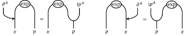
Figure 1: Eigenvalue equations of $q$-exponentials.

Using the operator representation in Eq. (30) of the last chapter, we found the following expressions for the $q$-exponentials of three-dimensional Euclidean quantum space [31]:

$$\exp_{q}(\mathbf{x}|\text{i}\mathbf{p}) =\sum_{\underline{n}\,=\,0}^{\infty}\frac{(x^{+})^{n_{+}}(x^{3})^{n_{3}}(x^{-})^{n_{-}}(\text{i}p_{-})^{n_{-}}(\text{i}p_{3})^{n_{3}}(\text{i}p_{+})^{n_{+}}}{[[\hskip 0.72229ptn_{+}]]_{q^{4}}!\,[[\hskip 0.72229ptn_{3}]]_{q^{2}}!\,[[\hskip 0.72229ptn_{-}]]_{q^{4}}!},$$

$$\exp_{q}(\text{i}^{-1}\mathbf{p}|\mathbf{x}) =\sum_{\underline{n}\,=\,0}^{\infty}\frac{(\text{i}^{-1}p^{+})^{n_{+}}(\text{i}^{-1}p^{3})^{n_{3}}(\text{i}^{-1}p^{-})^{n_{-}}(x_{-})^{n_{-}}(x_{3})^{n_{3}}(x_{+})^{n_{+}}}{[[\hskip 0.72229ptn_{+}]]_{q^{4}}!\,[[\hskip 0.72229ptn_{3}]]_{q^{2}}!\,[[\hskip 0.72229ptn_{-}]]_{q^{4}}}.$$ (50)

If we substitute $q$ with $q^{-1}$ in both expressions of Eq. (50), we get two more $q$-exponentials, which we designate $\overline{\exp}_{q}(x|$i$\mathbf{p})$ and $\overline{\exp}_{q}($i${}^{-1}\mathbf{p}|x)$. We obtain the eigenvalue equations and normalization conditions of these two $q$-exponentials by applying the following substitutions to Eqs. (48) and (49):

$$\exp_{q}\rightarrow\hskip 0.72229pt\overline{\exp}_{q},\qquad\triangleright\,\rightarrow\,\bar{\triangleright},\qquad\bar{\triangleleft}\,\rightarrow\,\triangleleft,\qquad\partial^{A}\rightarrow\hat{\partial}^{A}.$$ (51)

We can use $q$-exponentials to generate $q$-translations [32]. If we replace the momentum coordinates in the expressions for $q$-exponentials with derivatives, it applies [12, 29, 13]

$$\exp_{q}(x|\partial_{y})\triangleright g(\hskip 0.72229pty) =g(x\,\bar{\oplus}\,y),$$

$$\overline{\exp}_{q}(x|\hat{\partial}_{y})\,\bar{\triangleright}\,g(\hskip 0.72229pty) =g(x\oplus y),$$ (52)

and

$$g(\hskip 0.72229pty)\,\bar{\triangleleft}\,\exp_{q}(-\hskip 0.72229pt\partial_{y}|\hskip 0.72229ptx) =g(\hskip 0.72229pty\,\bar{\oplus}\,x),$$

$$g(\hskip 0.72229pty)\triangleleft\hskip 0.72229pt\overline{\exp}_{q}(-\hskip 0.72229pt\hat{\partial}_{y}|\hskip 0.72229ptx) =g(\hskip 0.72229pty\oplus x).$$ (53)

In the case of the three-dimensional $q$-deformed Euclidean space, for example, we can get the following formula for calculating $q$-translations [33]:

$$f(\mathbf{x}\oplus\mathbf{y})= \sum_{i_{+}=\hskip 0.72229pt0}^{\infty}\sum_{i_{3}=\hskip 0.72229pt0}^{\infty}\sum_{i_{-}=\hskip 0.72229pt0}^{\infty}\sum_{k\hskip 0.72229pt=\hskip 0.72229pt0}^{i_{3}}\frac{(-q^{-1}\lambda\lambda_{+})^{k}}{[[2k]]_{q^{-2}}!!}\frac{(x^{-})^{i_{-}}(x^{3})^{i_{3}-\hskip 0.72229ptk}(x^{+})^{i_{+}+\hskip 0.72229ptk}\,(\hskip 0.72229pty^{-})^{k}}{[[i_{-}]]_{q^{-4}}!\,[[i_{3}-k]]_{q^{-2}}!\,[[i_{+}]]_{q^{-4}}!}$$

$$\qquad\times\big{(}D_{q^{-4},\hskip 0.72229pty^{-}}^{i_{-}}D_{q^{-2},\hskip 0.72229pty^{3}}^{i_{3}+\hskip 0.72229ptk}\hskip 0.72229ptD_{q^{-4},\hskip 0.72229pty^{+}}^{i_{+}}f\big{)}(q^{2(k\hskip 0.72229pt-\hskip 0.72229pti_{3})}y^{-},q^{-2i_{+}}y^{3}).$$ (54)

In analogy to the undeformed case, $q$-exponentials satisfy addition theorems [29, 30, 13]. Concretely, we have

$$\exp_{q}(\mathbf{x}\,\bar{\oplus}\,\mathbf{y}|\text{i}\mathbf{p}) =\exp_{q}(\mathbf{x}|\exp_{q}(\hskip 0.72229pt\mathbf{y}|\text{i}\mathbf{p})\circledast\text{i}\mathbf{p}),$$

$$\exp_{q}(\text{i}\mathbf{x}|\mathbf{p}\,\bar{\oplus}\,\mathbf{p}^{\prime}) =\exp_{q}(\mathbf{x}\circledast\exp_{q}(\mathbf{x}|\hskip 0.72229pt\text{i}\mathbf{p})|\hskip 0.72229pt\text{i}\mathbf{p}^{\prime}),$$ (55)

and

$$\overline{\exp}_{q}(\mathbf{x}\oplus\mathbf{y}|\text{i}\mathbf{p}) =\overline{\exp}_{q}(\mathbf{x}|\overline{\exp}_{q}(\hskip 0.72229pt\mathbf{y}|\text{i}\mathbf{p})\circledast\text{i}\mathbf{p}),$$

$$\overline{\exp}_{q}(\text{i}\mathbf{x}|\mathbf{p}\oplus\mathbf{p}^{\prime}) =\overline{\exp}_{q}(\mathbf{x}\circledast\overline{\exp}_{q}(\mathbf{x}|\text{i}\mathbf{p})|\hskip 0.72229pt\text{i}\mathbf{p}^{\prime}).$$ (56)

We can obtain further addition theorems from the above identities by substituting position coordinates with momentum coordinates and vice versa. For a better understanding of the meaning of the two addition theorems in Eq. (55), we have given their graphic representation in Fig. 2.

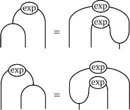
Figure 2: Addition theorems for $q$-exponentials.

The $q$-deformed quantum spaces considered so far are so-called braided Hopf algebras [34]. From this point of view, the two versions of $q$-translations are nothing else but realizations of two braided co-products $\underline{\Delta}$ and $\underline{\bar{\Delta}}$ on the corresponding commutative coordinate algebras [13]:

$$f(\mathbf{x}\oplus\mathbf{y}) =((\mathcal{W}^{\hskip 0.72229pt-1}\otimes\mathcal{W}^{\hskip 0.72229pt-1})\circ\underline{\Delta})(\mathcal{W}(f)),$$

$$f(\mathbf{x}\,\bar{\oplus}\,\mathbf{y}) =((\mathcal{W}^{\hskip 0.72229pt-1}\otimes\mathcal{W}^{-1})\circ\underline{\bar{\Delta}})(\mathcal{W}(f)).$$ (57)

The braided Hopf algebras have braided antipodes $\underline{S}$ and $\underline{\bar{S}}$ as well. We can realize these antipodes on the corresponding commutative algebras, too:

$$f(\ominus\,\mathbf{x}) =(\mathcal{W}^{\hskip 0.72229pt-1}\circ\underline{S}\hskip 0.72229pt)(\mathcal{W}(f)),$$

$$f(\bar{\ominus}\,\mathbf{x}) =(\mathcal{W}^{\hskip 0.72229pt-1}\circ\underline{\bar{S}}\hskip 0.72229pt)(\mathcal{W}(f)).$$ (58)

In the following, we refer to the operations in Eq. (58) as $q$-inversions. In the case of the $q$-deformed Euclidean space, for example, we have found the following operator representation for $q$-inversions [33]:

$$\hat{U}^{-1}f(\ominus\,\mathbf{x})= \sum_{i=0}^{\infty}(-\hskip 0.72229ptq\lambda\lambda_{+})^{i}\,\frac{(x^{+}x^{-})^{i}}{[[2i]]_{q^{-2}}!!}\,q^{-2\hat{n}_{+}(\hat{n}_{+}+\hskip 0.72229pt\hat{n}_{3})-2\hat{n}_{-}(\hat{n}_{-}+\hskip 0.72229pt\hat{n}_{3})-\hat{n}_{3}\hat{n}_{3}}$$

$$\qquad\times D_{q^{-2},\hskip 0.72229ptx^{3}}^{2i}\,f(-\hskip 0.72229ptq^{2-4i}x^{-},-\hskip 0.72229ptq^{1-2i}x^{3},-\hskip 0.72229ptq^{2-4i}x^{+}).$$ (59)

The operators $\hat{U}$ and $\hat{U}^{-1}$ act on a commutative function $f(x^{+},x^{3},x^{-})$ as follows:

$$\hat{U}f =\sum_{k\hskip 0.72229pt=\hskip 0.72229pt0}^{\infty}\left(-\lambda\right)^{k}\frac{(x^{3})^{2k}}{[[k]]_{q^{-4}}!}\,q^{-2\hat{n}_{3}(\hat{n}_{+}+\hskip 0.72229pt\hat{n}_{-}+\hskip 0.72229ptk)}D_{q^{-4},\hskip 0.72229ptx^{+}}^{k}D_{q^{-4},\hskip 0.72229ptx^{-}}^{k}f,$$

$$\hat{U}^{-1}f =\sum_{k\hskip 0.72229pt=\hskip 0.72229pt0}^{\infty}\lambda^{k}\hskip 0.72229pt\frac{(x^{3})^{2k}}{[[k]]_{q^{4}}!}\,q^{2\hat{n}_{3}(\hat{n}_{+}+\hskip 0.72229pt\hat{n}_{-}+\hskip 0.72229ptk)}D_{q^{4},\hskip 0.72229ptx^{+}}^{k}D_{q^{4},\hskip 0.72229ptx^{-}}^{k}f.$$ (60)

The braided co-products and braided antipodes satisfy the axioms (also see Ref. [34])

$$m\circ(\underline{S}\otimes\operatorname*{id})\circ\underline{\Delta} =m\circ(\operatorname*{id}\otimes\,\underline{S}\hskip 0.72229pt)\circ\underline{\Delta}=\underline{\varepsilon},$$

$$m\circ(\underline{\bar{S}}\otimes\operatorname*{id})\circ\underline{\bar{\Delta}} =m\circ(\operatorname*{id}\otimes\,\underline{\bar{S}}\hskip 0.72229pt)\circ\underline{\bar{\Delta}}=\underline{\bar{\varepsilon}},$$ (61)

and

$$(\operatorname*{id}\otimes\,\underline{\varepsilon})\circ\underline{\Delta} =\operatorname*{id}=(\underline{\varepsilon}\otimes\operatorname*{id})\circ\underline{\Delta},$$

$$(\operatorname*{id}\otimes\,\underline{\bar{\varepsilon}})\circ\underline{\bar{\Delta}} =\operatorname*{id}=(\underline{\bar{\varepsilon}}\otimes\operatorname*{id})\circ\underline{\bar{\Delta}}.$$ (62)

In the identities above, we denote the operation of multiplication on the braided Hopf algebra by $m$. The co-units $\underline{\varepsilon},\underline{\bar{\varepsilon}}$ of the two braided Hopf structures are both linear mappings vanishing on the coordinate generators:

$$\varepsilon(X^{i})=\underline{\bar{\varepsilon}}(X^{i})=0.$$ (63)

For this reason, we can realize the co-units $\underline{\varepsilon}$ and $\underline{\bar{\varepsilon}}$ on a commutative coordinate algebra as follows:

$$\underline{\varepsilon}(\mathcal{W}(f))=\underline{\bar{\varepsilon}}(\mathcal{W}(f))=\left.f(\mathbf{x})\right|_{x\hskip 0.72229pt=\hskip 0.72229pt0}=f(0).$$ (64)

Next, we translate the Hopf algebra axioms in Eqs. (61) and (62) into corresponding rules for $q$-translations and $q$-inversions [13], i. e.

$$f((\ominus\,\mathbf{x})\oplus\mathbf{x}) =f(\mathbf{x}\oplus(\ominus\,\mathbf{x}))=f(0),$$

$$f((\bar{\ominus}\,\mathbf{x})\,\bar{\oplus}\,\mathbf{x}) =f(\mathbf{x}\,\bar{\oplus}\,(\bar{\ominus}\,\mathbf{x}))=f(0),$$ (65)

and

$$f(\mathbf{x}\oplus\mathbf{y})|_{y\hskip 0.72229pt=\hskip 0.72229pt0} =f(\mathbf{x})=f(\mathbf{y}\oplus\mathbf{x})|_{y\hskip 0.72229pt=\hskip 0.72229pt0},$$

$$f(\mathbf{x}\,\bar{\oplus}\,\mathbf{y})|_{y\hskip 0.72229pt=\hskip 0.72229pt0} =f(\mathbf{x})=f(\mathbf{y}\,\bar{\oplus}\,\mathbf{x})|_{y\hskip 0.72229pt=\hskip 0.72229pt0}.$$ (66)

Using $q$-inversions, we are also able to introduce inverse $q$-exponentials:

$$\exp_{q}(\bar{\ominus}\,\mathbf{x}|\text{i}\mathbf{p})=\exp_{q}(\text{i}\mathbf{x}|\text{{}}\bar{\ominus}\,\mathbf{p}).$$ (67)

Due to the addition theorems and the normalization conditions of our $q$-exponentials, the following applies:

$$\exp_{q}(\text{i}\mathbf{x}\circledast\exp_{q}(\bar{\ominus}\,\mathbf{x}|\hskip 0.72229pt\text{i}\mathbf{p})\circledast\mathbf{p})=\exp_{q}(\mathbf{x}\,\bar{\oplus}\,(\bar{\ominus}\,\mathbf{x})|\hskip 0.72229pt\text{i}\mathbf{p})=\exp_{q}(\mathbf{x}|\text{i}\mathbf{p})|_{x=0}=1.$$ (68)

For a better understanding of these identities, we have given their graphic representation in Fig. 3. You find some explanations of this sort of graphical calculations in Ref. [35].

Figure 3: Invertibility of $q$-exponentials.

The conjugate $q$-exponentials $\overline{\exp}_{q}$ are subject to similar rules obtained from the above identities by using the following substitutions:

$$\exp_{q}\rightarrow\overline{\exp}_{q},\qquad\bar{\oplus}\,\rightarrow\,\oplus,\qquad\bar{\ominus}\,\rightarrow\,\ominus.$$ (69)

Next, we describe another way of obtaining $q$-exponentials. We exchange the two tensor factors of a $q$-exponential using the inverse of the so-called universal R-matrix [also see the graphic representation in Fig. 4]:

$$\exp_{q}^{\ast}(\text{i}\mathbf{p}|\hskip 0.72229pt\mathbf{x}) =\tau\circ[(\mathcal{R}_{[2]}^{-1}\otimes\mathcal{R}_{[1]}^{-1})\triangleright\exp_{q}(\text{i}\mathbf{x}|\ominus\mathbf{p})],$$

$$\exp_{q}^{\ast}(\mathbf{x}|\text{i}\mathbf{p}) =\tau\circ[(\mathcal{R}_{[2]}^{-1}\otimes\mathcal{R}_{[1]}^{-1})\triangleright\exp_{q}(\ominus\hskip 1.4457pt\mathbf{p}|\hskip 0.72229pt\text{i}\mathbf{x})].$$ (70)

In the expressions above, $\tau$ denotes the ordinary twist operator. One can show that the new $q$-exponentials satisfy the following eigenvalue equations (see Fig. 4):

$$\exp_{q}^{\ast}(\text{i}\mathbf{p}|\hskip 0.72229pt\mathbf{x})\triangleleft\partial^{A} =\text{i}p^{A}\circledast\exp_{q}^{\ast}(\text{i}\mathbf{p}|\hskip 0.72229pt\mathbf{x}),$$

$$\partial^{A}\,\bar{\triangleright}\,\exp_{q}^{\ast}(\mathbf{x}|\text{i}^{-1}\mathbf{p}) =\exp_{q}^{\ast}(\mathbf{x}|\text{i}^{-1}\mathbf{p})\circledast\text{i}p^{A}.$$ (71)

Similar considerations apply to the conjugate $q$-exponentials. We only need to modify Eqs. (70) and (71) by performing the following substitutions:

$$\exp_{q}^{\ast}\rightarrow\overline{\exp}_{q}^{\ast},\qquad\mathcal{R}_{[2]}^{-1}\otimes\mathcal{R}_{[1]}^{-1}\rightarrow\mathcal{R}_{[1]}\otimes\mathcal{R}_{[2]},\qquad\ominus\,\rightarrow\,\bar{\ominus},$$

$$\bar{\triangleright}\,\rightarrow\,\triangleright,\qquad\triangleleft\,\rightarrow\,\bar{\triangleleft},\qquad\partial^{A}\rightarrow\hat{\partial}^{A}.$$ (72)

The $q$-exponentials in Eq. (70) are related to the conjugate $q$-exponentials. To see this, we rewrite the eigenvalue equations in (71) by using the identity $\hat{\partial}^{A}=q^{6}\partial^{A}$ as follows:

$$\exp_{q}^{\ast}(\text{i}\mathbf{p}|\hskip 0.72229pt\mathbf{x})\triangleleft\hat{\partial}^{A} =\text{i}q^{6}p^{A}\circledast\exp_{q}^{\ast}(\text{i}\mathbf{p}|\hskip 0.72229pt\mathbf{x}),$$

$$\hat{\partial}^{A}\,\bar{\triangleright}\,\exp_{q}^{\ast}(\mathbf{x}|\text{i}^{-1}\mathbf{p}) =\exp_{q}^{\ast}(\mathbf{x}|\text{i}^{-1}\mathbf{p})\circledast\text{i}q^{6}p^{A}.$$ (73)

These are the eigenvalue equations for $\overline{\exp}_{q}($i${}^{-1}q^{6}\mathbf{p}|\mathbf{x})$ and $\overline{\exp}_{q}(\mathbf{x}|$i$q^{6}\mathbf{p})$, so the following identifications are valid:

$$\exp_{q}^{\ast}(\text{i}\mathbf{p}|\mathbf{x})=\overline{\exp}_{q}(\text{i}^{-1}q^{6}\mathbf{p}|\mathbf{x}),\qquad\exp_{q}^{\ast}(\mathbf{x}|\hskip 0.72229pt\text{i}^{-1}\mathbf{p})=\overline{\exp}_{q}(\mathbf{x}|\text{i}q^{6}\mathbf{p}).$$ (74)

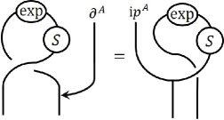
Figure 4: Eigenvalue equation of twisted $q$-exponential.

For the sake of completeness, we also write down how the $q$-exponentials of $q$-deformed Euclidean space behave under quantum space conjugation:

$$\overline{\exp_{q}(\mathbf{x}|\text{i}\mathbf{p})} =\exp_{q}(\text{i}^{-1}\mathbf{p}|\mathbf{x}), \overline{\overline{\exp}_{q}(\mathbf{x}|\text{i}\mathbf{p})} =\overline{\exp}_{q}(\text{i}^{-1}\mathbf{p}|\mathbf{x}),$$

$$\overline{\exp_{q}^{\ast}(\text{i}\mathbf{p}|\mathbf{x})} =\exp_{q}^{\ast}(\mathbf{x}|\text{i}^{-1}\mathbf{p}), \overline{\overline{\exp}_{q}^{\ast}(\text{i}\mathbf{p}|\mathbf{x})} =\overline{\exp}_{q}^{\ast}(\mathbf{x}|\text{i}^{-1}\mathbf{p}).$$ (75)

3 Hamilton operator for a free particle

Since the $q$-deformed Hamilton operator of a free nonrelativistic particle is supposed to be invariant under rotations, it must behave like a scalar concerning the action of the Hopf algebra $\mathcal{U}_{q}(\operatorname*{su}\nolimits_{2})$. For this reason, we choose the following expression as Hamilton operator for a free nonrelativistic particle with mass $m$:

$$H_{0}=-(2\hskip 0.72229ptm)^{-1}g_{AB}\hskip 0.72229pt\partial^{A}\partial^{B}=-(2\hskip 0.72229ptm)^{-1}\partial^{A}\partial_{A}.$$ (76)

Due to its definition, the Hamilton operator $H_{0}$ is a central element of the algebra of $q$-deformed partial derivatives:

$$[H_{0},\partial^{A}]=0,\quad A\in\{+,3,-\}.$$ (77)

The conjugation properties of the partial derivatives imply that $H_{0}$ is invariant under conjugation [cf. Eq. (25) of Chap. 2.2]:

$$\overline{H_{0}}=H_{0}.$$ (78)

We mention that $H_{0}$ results from the low-energy limit of the following energy-momentum relation:

$$E_{\mathbf{p}}^{\hskip 0.72229pt2}=c^{2}(\hskip 0.72229ptp^{A}p_{A}+(m\hskip 0.72229ptc)^{2}).$$ (79)

You can see this by the following calculation:

$$E_{\mathbf{p}} =c\hskip 0.72229pt\sqrt{p^{A}p_{A}+(m\hskip 0.72229ptc)^{2}}=m\hskip 0.72229ptc^{2}\sqrt{1+(m\hskip 0.72229ptc)^{-2}p^{A}p_{A}}$$

$$=m\hskip 0.72229ptc^{2}(1+2^{-1}(m\hskip 0.72229ptc)^{-2}p^{A}p_{A}+\ldots)$$

$$=m\hskip 0.72229ptc^{2}+(2\hskip 0.72229ptm)^{-1}p^{A}p_{A}+\ldots$$ (80)

The second term of the last expression in Eq. (80) gives $H_{0}$ if we replace the momentum variable $p^{A}$ with the operator i${}^{-1}\partial^{A}$.

4 Solutions to the free Schrödinger equations

In Ref. [15], we have derived Schrödinger equations for the three-dimensional $q$-deformed Euclidean space $\mathbb{R}_{q}^{3}$. Now we want to find solutions to these Schrödinger equations with the free Hamilton operator given by the expression in Eq. (76) of the previous chapter:

$$\text{i}\partial_{t}\triangleright\phi_{R}(\mathbf{x},t) =H_{0}\triangleright\phi_{R}(\mathbf{x},t),$$

$$\phi_{L}^{\ast}(\mathbf{x},t)\triangleleft\partial_{t}\text{i} =\phi_{L}^{\ast}(\mathbf{x},t)\triangleleft H_{0}.$$ (81)

Due to Eq. (77) of the previous chapter, the free Hamilton operator commutes with the momentum operator i${}^{-1}\partial_{A}$. So we seek solutions that are eigenfunctions of the momentum operator ($A\in\{+,3,-\}$):

$$\text{i}^{-1}\partial_{A}\triangleright u_{\hskip 0.72229pt\mathbf{p}}(\mathbf{x},t) =u_{\hskip 0.72229pt\mathbf{p}}(\mathbf{x},t)\circledast p_{A},$$

$$(u^{\ast})_{\mathbf{p}}(\mathbf{x},t)\triangleleft\partial_{A}\text{i}^{-1} =p_{A}\circledast(u^{\ast})_{\mathbf{p}}(\mathbf{x},t).$$ (82)

Resulting from these identities, we can write the Schrödinger equation for the wave function $u_{\hskip 0.72229pt\mathbf{p}}(\mathbf{x},t)$ or $(u^{\ast})_{\mathbf{p}}(\mathbf{x},t)$ as follows:

$$\text{i}\partial_{t}\triangleright u_{\hskip 0.72229pt\mathbf{p}}(\mathbf{x},t) =H_{0}\triangleright u_{\hskip 0.72229pt\mathbf{p}}(\mathbf{x},t)=-(2\hskip 0.72229ptm)^{-1}\hskip 0.72229pt\partial^{A}\partial_{A}\triangleright u_{\hskip 0.72229pt\mathbf{p}}(\mathbf{x},t)$$

$$=u_{\hskip 0.72229pt\mathbf{p}}(\mathbf{x},t)\circledast\mathbf{p}^{2}(2\hskip 0.72229ptm)^{-1},$$ (83)

$$(u^{\ast})_{\mathbf{p}}(\mathbf{x},t)\triangleleft\partial_{t}\text{i} =(u^{\ast})_{\mathbf{p}}(\mathbf{x},t)\triangleleft H_{0}=-(u^{\ast})_{\mathbf{p}}(\mathbf{x},t)\triangleleft\partial^{A}\partial_{A}(2\hskip 0.72229ptm)^{-1}$$

$$=(2\hskip 0.72229ptm)^{-1}\hskip 0.72229pt\mathbf{p}^{2}\circledast(u^{\ast})_{\mathbf{p}}(\mathbf{x},t).$$ (84)

The equations above show us that $u_{\hskip 0.72229pt\mathbf{p}}(\mathbf{x},t)$ and $(u^{\ast})_{\mathbf{p}}(\mathbf{x},t)$ are eigenfunctions of the energy operator as well.

To find expressions for the functions $u_{\hskip 0.72229pt\mathbf{p}}(\mathbf{x},t)$ and $(u^{\ast})_{\mathbf{p}}(\mathbf{x},t)$, we consider the $q$-deformed momentum eigenfunctions introduced in Ref. [14]. These momentum eigenfunctions satisfy the following eigenvalue equations:

$$\text{i}^{-1}\partial^{A}\triangleright u_{\hskip 0.72229pt\mathbf{p}}(\mathbf{x}) =u_{\hskip 0.72229pt\mathbf{p}}(\mathbf{x})\circledast p^{A}, u^{\mathbf{p}}(\mathbf{x})\,\bar{\triangleleft}\,\partial^{A}\hskip 0.72229pt\text{i}^{-1} =p^{A}\circledast u^{\mathbf{p}}(\mathbf{x}),$$

$$\text{i}^{-1}\hat{\partial}^{A}\,\bar{\triangleright}\,\bar{u}_{\hskip 0.72229pt\mathbf{p}}(\mathbf{x}) =\bar{u}_{\hskip 0.72229pt\mathbf{p}}(\mathbf{x})\circledast p^{A}, \bar{u}^{\mathbf{p}}(\mathbf{x})\triangleleft\hat{\partial}^{A}\hskip 0.72229pt\text{i}^{-1} =p^{A}\circledast\bar{u}^{\mathbf{p}}(\mathbf{x}).$$ (85)

Since the $q$-exponentials of Chap. 2.3 are eigenfunctions of $q$-deformed partial derivatives, the $q$-deformed momentum eigenfunctions can take on the following form:

$$u_{\hskip 0.72229pt\mathbf{p}}(\mathbf{x}) =\operatorname*{vol}\nolimits^{-1/2}\exp_{q}(\mathbf{x}|\text{i}\mathbf{p}), u^{\mathbf{p}}(\mathbf{x}) =\operatorname*{vol}\nolimits^{-1/2}\exp_{q}(\text{i}^{-1}\mathbf{p}|\hskip 0.72229pt\mathbf{x}),$$

$$\bar{u}_{\hskip 0.72229pt\mathbf{p}}(\mathbf{x}) =\operatorname*{vol}\nolimits^{-1/2}\overline{\exp}_{q}(\mathbf{x}|\text{i}\mathbf{p}), \bar{u}^{\mathbf{p}}(\mathbf{x}) =\operatorname*{vol}\nolimits^{-1/2}\overline{\exp}_{q}(\text{i}^{-1}\mathbf{p}|\hskip 0.72229pt\mathbf{x}).$$ (86)

The volume element $\operatorname*{vol}$ is defined by the expression in Eq. (116) of the next chapter. We can also introduce dual momentum eigenfunctions [cf. Eq. (70) of Chap. 2.3]:

$$(u^{\ast})_{\mathbf{p}}(\mathbf{x}) =\operatorname*{vol}\nolimits^{-1/2}\exp_{q}^{\ast}(\text{i}\mathbf{p}|\hskip 0.72229pt\mathbf{x}), (u^{\ast})^{\mathbf{p}}(\mathbf{x}) =\operatorname*{vol}\nolimits^{-1/2}\exp_{q}^{\ast}(\mathbf{x}|\text{i}^{-1}\mathbf{p}),$$

$$(\bar{u}^{\ast})_{\mathbf{p}}(\mathbf{x}) =\operatorname*{vol}\nolimits^{-1/2}\overline{\exp}_{q}^{\ast}(\text{i}\mathbf{p}|\hskip 0.72229pt\mathbf{x}), (\bar{u}^{\ast})^{\mathbf{p}}(\mathbf{x}) =\operatorname*{vol}\nolimits^{-1/2}\overline{\exp}_{q}^{\ast}(\mathbf{x}|\text{i}^{-1}\mathbf{p}).$$ (87)

The corresponding eigenvalue equations are given by [cf. Eq. (71) of Chap. 2.3]

$$(u^{\ast})_{\mathbf{p}}(\mathbf{x})\triangleleft\partial^{A}\hskip 0.72229pt\text{i}^{-1} =p^{A}\circledast(u^{\ast})_{\mathbf{p}}(\mathbf{x}),$$

$$\text{i}^{-1}\partial^{A}\,\bar{\triangleright}\,(u^{\ast})^{\mathbf{p}}(\mathbf{x}) =(u^{\ast})^{\mathbf{p}}(\mathbf{x})\circledast p^{A},$$ (88)

or

$$(\bar{u}^{\ast})_{\mathbf{p}}(\mathbf{x})\,\bar{\triangleleft}\,\hat{\partial}^{A}\hskip 0.72229pt\text{i}^{-1} =p^{A}\circledast(\bar{u}^{\ast})_{\mathbf{p}}(\mathbf{x}),$$

$$\text{i}^{-1}\hat{\partial}^{A}\triangleright(\bar{u}^{\ast})^{\mathbf{p}}(\mathbf{x}) =(\bar{u}^{\ast})^{\mathbf{p}}(\mathbf{x})\circledast p^{A}.$$ (89)

In what follows, we restrict our considerations to the momentum eigenfunctions $u_{\hskip 0.72229pt\mathbf{p}}(\mathbf{x})$ and $(u^{\ast})_{\mathbf{p}}(\mathbf{x})$.  We can obtain the results for the other momentum eigenfunctions by simple substitutions specified at the end of this chapter.

We have shown in Ref. [15] that the time evolution operator for the quantum space $\mathbb{R}_{q}^{3}$ is of the same form as in the undeformed case. For this reason, we get solutions to our $q$-deformed Schrödinger equations by applying the operators $\exp(-$i$tH_{0})$ and $\exp($i$tH_{0})$ to time-independent functions $\phi_{R}(\mathbf{x},0)$ and $\phi_{L}^{\ast}(\mathbf{x},0)$:

$$\phi_{R}(\mathbf{x},t) =\exp(-\text{i}tH_{0})\triangleright\phi_{R}(\mathbf{x},0),$$

$$\phi_{L}^{\ast}(\mathbf{x},t) =\phi_{L}^{\ast}(\mathbf{x},0)\triangleleft\exp(\text{i}H_{0}t).$$ (90)

In the same way, we can obtain plane wave solutions to our Schrödinger equations from the momentum eigenfunctions $u_{\hskip 0.72229pt\mathbf{p}}(\mathbf{x})$ and $(u^{\ast})_{\mathbf{p}}(\mathbf{x})$, i. e.

$$u_{\hskip 0.72229pt\mathbf{p}}(\mathbf{x},t) =\exp(-\text{i}tH_{0})\triangleright u_{\hskip 0.72229pt\mathbf{p}}(\mathbf{x})=u_{\hskip 0.72229pt\mathbf{p}}(\mathbf{x})\circledast\exp(-\text{i}t\hskip 0.72229pt\mathbf{p}^{2}(2\hskip 0.72229ptm)^{-1})$$

$$=\operatorname*{vol}\nolimits^{-1/2}\exp_{q}(\mathbf{x}|\text{i}\mathbf{p})\circledast\exp(-\text{i}t\hskip 0.72229pt\mathbf{p}^{2}(2\hskip 0.72229ptm)^{-1}),$$ (91)

and

$$(u^{\ast})_{\mathbf{p}}(\mathbf{x},t) =(u^{\ast})_{\mathbf{p}}(\mathbf{x})\triangleleft\exp(\text{i}H_{0}t)=\exp(\text{i}t\hskip 0.72229pt\mathbf{p}^{2}(2\hskip 0.72229ptm)^{-1})\circledast(u^{\ast})_{\mathbf{p}}(\mathbf{x})$$

$$=\operatorname*{vol}\nolimits^{-1/2}\exp(\text{i}t\hskip 0.72229pt\mathbf{p}^{2}(2\hskip 0.72229ptm)^{-1})\circledast\exp_{q}^{\ast}(\text{i}\mathbf{p|\hskip 0.72229ptx}).$$ (92)

The momentum eigenfunctions are multiplied by a time-dependent phase factor if the time evolution operator acts on them. This phase factor is given by

$$\exp(\pm\hskip 0.72229pt\text{i}t\hskip 0.72229pt\mathbf{p}^{2}(2\hskip 0.72229ptm)^{-1})=\sum_{k\hskip 0.72229pt=\hskip 0.72229pt0}^{\infty}\frac{1}{k!}\left(\pm\hskip 0.72229pt\text{i}t(2\hskip 0.72229ptm)^{-1}\right)^{k}\mathbf{p}^{2k},$$ (93)

where powers of $\mathbf{p}^{2}(=g^{AB}\hskip 1.4457ptp_{A}\circledast p_{B})$ are calculated by using the star-product:

$$\mathbf{p}^{2k}=\hskip 0.72229pt\overset{k-\text{times}}{\overbrace{\mathbf{p}^{2}\circledast\ldots\circledast\mathbf{p}^{2}}}\hskip 0.72229pt=\sum_{l\hskip 0.72229pt=\hskip 0.72229pt0}^{k}\hskip 0.72229pt(C_{q})_{l}^{k}\,(\hskip 0.72229ptp_{-})^{k-l}(\hskip 0.72229ptp_{3})^{2l}(\hskip 0.72229ptp_{+})^{k-l},$$ (94)

The coefficients $(C_{q})_{l}^{k}$ in the series expansion above satisfy the following recurrence relation ($\lambda_{+}=q+q^{-1}$):

$$(C_{q})_{l}^{k}=-\lambda_{+}\hskip 1.4457ptq^{4l}(C_{q})_{l}^{k\hskip 0.72229pt-1}+q^{-2}(C_{q})_{l\hskip 0.72229pt-1}^{k\hskip 0.72229pt-1}.$$ (95)

As you can verify by inserting, this recurrence relation has the following solution:

$$(C_{q})_{l}^{k}=q^{-2l}(-\lambda_{+})^{k-l}\genfrac{[}{]}{0.0pt}{}{k}{l}_{q^{4}}.$$ (96)

The $q$-deformed binomial coefficients are defined in complete analogy to the undeformed case:

$$\genfrac{[}{]}{0.0pt}{}{n}{k}_{q}=\frac{[[\hskip 0.72229ptn]]_{q}!}{[[\hskip 0.72229ptn-k]]_{q}!\hskip 0.72229pt[[k]]_{q}!}.$$ (97)

Combining our results, we finally get:

$$\exp(\pm\hskip 0.72229pt\text{i}t\hskip 0.72229pt\mathbf{p}^{2}(2\hskip 0.72229ptm)^{-1})=$$

$$=\sum_{k\hskip 0.72229pt=\hskip 0.72229pt0}^{\infty}\frac{1}{k!}\left(\frac{\pm\hskip 0.72229pt\text{i}t}{2\hskip 0.72229ptm}\right)^{k}\sum_{l\hskip 0.72229pt=\hskip 0.72229pt0}^{k}q^{-2l}(-\lambda_{+})^{k-l}\genfrac{[}{]}{0.0pt}{}{k}{l}_{q^{4}}(\hskip 0.72229ptp_{-})^{k-l}(\hskip 0.72229ptp_{3})^{2l}(\hskip 0.72229ptp_{+})^{k-l}$$

$$=\sum_{k\hskip 0.72229pt=\hskip 0.72229pt0}^{\infty}\frac{1}{k!}\left(\frac{\mp\hskip 0.72229pt\text{i}t\lambda_{+}}{2\hskip 0.72229ptm}\hskip 0.72229ptp_{-}p_{+}\right)^{k}\frac{1}{((\hskip 0.72229ptp_{3})^{2}/(-\hskip 0.72229ptq^{2}\lambda_{+}\hskip 0.72229ptp_{-}p_{+});q^{4})_{k}}.$$ (98)

The second identity is a consequence of Heine’s binomial formula [36]:

$$\frac{1}{(z\hskip 0.72229pt;q)_{k}}=\frac{1}{(1-z)(1-z\hskip 0.72229ptq)\ldots(1-z\hskip 0.72229ptq^{k-1})}=\sum_{l\hskip 0.72229pt=\hskip 0.72229pt0}^{k}\genfrac{[}{]}{0.0pt}{}{k}{l}_{q}\hskip 0.72229ptz^{l}.$$ (99)

Due to Eqs. (91) and (92), we must calculate the star-product of the time-dependent phase factor and the time-independent momentum eigenfunction in the end. To get an expression for $u_{\hskip 0.72229pt\mathbf{p}}(\mathbf{x},t)$, for example, we proceed as follows:

$$\hskip 0.72229pt\mathbf{p}^{2k}\circledast(\hskip 0.72229ptp_{-})^{n_{-}}(\hskip 0.72229ptp_{3})^{n_{3}}(\hskip 0.72229ptp_{+})^{n_{+}}=\,(\hskip 0.72229ptp_{-})^{n_{-}}\circledast\mathbf{p}^{2k}\circledast(\hskip 0.72229ptp_{3})^{n_{3}}(\hskip 0.72229ptp_{+})^{n_{+}}$$

$$\qquad=\,\sum_{l\hskip 0.72229pt=\hskip 0.72229pt0}^{k}\hskip 0.72229pt(C_{q})_{l}^{k}\,(\hskip 0.72229ptp_{-})^{n_{-}+\hskip 0.72229ptk-l}(\hskip 0.72229ptp_{3})^{2l}(\hskip 0.72229ptp_{+})^{k-l}\circledast(\hskip 0.72229ptp_{3})^{n_{3}}(\hskip 0.72229ptp_{+})^{n_{+}}$$

$$\qquad=\,\sum_{l\hskip 0.72229pt=\hskip 0.72229pt0}^{k}\hskip 0.72229ptq^{2n_{3}(k-l)}(C_{q})_{l}^{k}\,(\hskip 0.72229ptp_{-})^{n_{-}+\hskip 0.72229ptk-l}(\hskip 0.72229ptp_{3})^{n_{3}+2l}(\hskip 0.72229ptp_{+})^{n_{+}+\hskip 0.72229ptk-l}.$$ (100)

In the first step of the calculation above, we have used the fact that $\mathbf{p}^{2}$ is a central element of the momentum algebra. In the second step, we have inserted the expression given in Eq. (94). The last step follows from Eq. (16) in Chap. 2.1 if we take into account that $p_{A}=g_{AB}\hskip 0.72229ptp^{B}$. With the result of Eq. (100), we obtain from Eqs. (91) and (93) together with Eq. (50) of Chap. 2.3 the following expression for $u_{\hskip 0.72229pt\mathbf{p}}(\mathbf{x},t)$:

$$u_{\hskip 0.72229pt\mathbf{p}}(\mathbf{x},t)= \operatorname*{vol}\nolimits^{-1/2}\sum_{\underline{n}\hskip 0.72229pt=\hskip 0.72229pt0}^{\infty}\sum_{k\hskip 0.72229pt=\hskip 0.72229pt0}^{\infty}\sum_{l\hskip 0.72229pt=\hskip 0.72229pt0}^{k}\frac{(-\lambda_{+})^{k-l}q^{-2l+2n_{3}(k-l)}}{k!\,[[\hskip 0.72229ptn_{+}]]_{q^{4}}!\,[[\hskip 0.72229ptn_{3}]]_{q^{2}}!\,[[\hskip 0.72229ptn_{-}]]_{q^{4}}!}\,\genfrac{[}{]}{0.0pt}{}{k}{l}_{q^{4}}$$

$$\qquad\quad\times(2\hskip 0.72229ptm)^{-k}(\text{i}t)^{k}(x^{+})^{n_{+}}(x^{3})^{n_{3}}(x^{-})^{n_{-}}$$

$$\qquad\quad\times(\text{i}p_{-})^{n_{-}+\hskip 0.72229ptk-l}(\text{i}p_{3})^{n_{3}+2l}(\text{i}p_{+})^{n_{+}+\hskip 0.72229ptk-l}.$$ (101)

The time-dependent phase factor depends on $\mathbf{p}^{2}$. Thus the phase factor is a central element of the $q$-deformed momentum algebra. With this insight, we can show that our plane wave solutions are momentum eigenfunctions as well [also see Eq. (82)]:

$$\text{i}^{-1}\partial_{A}\triangleright u_{\hskip 0.72229pt\mathbf{p}}(\mathbf{x},t) =\text{i}^{-1}\partial_{A}\triangleright u_{\hskip 0.72229pt\mathbf{p}}(\mathbf{x})\circledast\exp\left(-\text{i}t\hskip 0.72229pt\mathbf{p}^{2}(2\hskip 0.72229ptm)^{-1}\right)$$

$$=u_{\hskip 0.72229pt\mathbf{p}}(\mathbf{x})\circledast p_{A}\circledast\exp\left(-\text{i}t\hskip 0.72229pt\mathbf{p}^{2}(2\hskip 0.72229ptm)^{-1}\right)$$

$$=u_{\hskip 0.72229pt\mathbf{p}}(\mathbf{x})\circledast\exp\left(-\text{i}t\hskip 0.72229pt\mathbf{p}^{2}(2\hskip 0.72229ptm)^{-1}\right)\circledast p_{A}=u_{\hskip 0.72229pt\mathbf{p}}(\mathbf{x},t)\circledast p_{A}.$$ (102)

By quantum space conjugation, you can obtain further $q$-deformed Schrödinger equations from Eq. (81), i. e. [also see Eq. (36) of Chap. 2.2]

$$\phi_{L}(\mathbf{x},t)\,\bar{\triangleleft}\,\partial_{t}\text{i} =\phi_{L}(\mathbf{x},t)\,\bar{\triangleleft}\,H_{0},$$

$$\text{i}\partial_{t}\,\bar{\triangleright}\,\phi_{R}^{\ast}(\mathbf{x},t) =H_{0}\,\bar{\triangleright}\,\phi_{R}^{\ast}(\mathbf{x},t)$$ (103)

with

$$\overline{\phi_{R}(\mathbf{x},t)}=\phi_{L}(\mathbf{x},t),\qquad\overline{\phi_{L}^{\ast}(\mathbf{x},t)}=\phi_{R}^{\ast}(\mathbf{x},t).$$ (104)

Accordingly, the quantum space conjugates of the plane waves $u_{\hskip 0.72229pt\mathbf{p}}(\mathbf{x},t)$ and $(u^{\ast})_{\mathbf{p}}(\mathbf{x},t)$ are plane wave solutions to the $q$-deformed Schrödinger equations given in Eq. (103), i. e.

$$u^{\mathbf{p}}(\mathbf{x},t)\,\bar{\triangleleft}\,\partial_{t}\text{i} =u^{\mathbf{p}}(\mathbf{x},t)\,\bar{\triangleleft}\,H_{0}=(2\hskip 0.72229ptm)^{-1}\mathbf{p}^{2}\circledast u^{\mathbf{p}}(\mathbf{x},t),$$

$$\text{i}\partial_{t}\,\bar{\triangleright}\,(u^{\ast})^{\mathbf{p}}(\mathbf{x},t) =H_{0}\,\bar{\triangleright}\,(u^{\ast})^{\mathbf{p}}(\mathbf{x},t)=(u^{\ast})^{\mathbf{p}}(\mathbf{x},t)\circledast\mathbf{p}^{2}(2\hskip 0.72229ptm)^{-1}$$ (105)

with

$$u^{\mathbf{p}}(\mathbf{x},t)=\overline{u_{\hskip 0.72229pt\mathbf{p}}(\mathbf{x},t)},\qquad(u^{\ast})^{\mathbf{p}}(\mathbf{x},t)=\overline{(u^{\ast})_{\mathbf{p}}(\mathbf{x},t)}.$$ (106)

The new plane wave solutions are subject to the identities

$$u^{\mathbf{p}}(\mathbf{x},t) =u^{\mathbf{p}}(\mathbf{x})\,\bar{\triangleleft}\,\exp(\text{i}H_{0}t)$$

$$=\exp\left(\text{i}t\hskip 0.72229pt\mathbf{p}^{2}(2\hskip 0.72229ptm)^{-1}\right)\circledast u^{\mathbf{p}}(\mathbf{x})$$

$$=\exp\left(\text{i}t\hskip 0.72229pt\mathbf{p}^{2}(2\hskip 0.72229ptm)^{-1}\right)\circledast\exp_{q}(\text{i}^{-1}\mathbf{p}|\hskip 0.72229pt\mathbf{x})\operatorname*{vol}\nolimits^{-1/2}$$ (107)

and

$$(u^{\ast})^{\mathbf{p}}(\mathbf{x},t) =\exp(-\text{i}tH_{0})\,\bar{\triangleright}\,(u^{\ast})^{\mathbf{p}}(\mathbf{x})$$

$$=(u^{\ast})^{\mathbf{p}}(\mathbf{x})\circledast\exp\left(-\text{i}t\hskip 0.72229pt\mathbf{p}^{2}(2\hskip 0.72229ptm)^{-1}\right)$$

$$=\operatorname*{vol}\nolimits^{-1/2}\exp_{q}^{\ast}(\mathbf{x}|\text{i}^{-1}\mathbf{p})\circledast\exp\left(-\text{i}t\hskip 0.72229pt\mathbf{p}^{2}(2\hskip 0.72229ptm)^{-1}\right).$$ (108)

Last not but least, we write down an explicit formula for $u^{\mathbf{p}}(\mathbf{x},t)$:

$$u^{\mathbf{p}}(\mathbf{x},t)= \operatorname*{vol}\nolimits^{-1/2}\sum_{\underline{n}\hskip 0.72229pt=\hskip 0.72229pt0}^{\infty}\sum_{k\hskip 0.72229pt=\hskip 0.72229pt0}^{\infty}\sum_{l\hskip 0.72229pt=\hskip 0.72229pt0}^{k}\frac{(-\lambda_{+})^{k-l}q^{-2l+2n_{3}(k-l)}}{k!\,[[\hskip 0.72229ptn_{+}]]_{q^{4}}!\,[[\hskip 0.72229ptn_{3}]]_{q^{2}}!\,[[\hskip 0.72229ptn_{-}]]_{q^{4}}!}\,\genfrac{[}{]}{0.0pt}{}{k}{l}_{q^{4}}$$

$$\qquad\quad\times(2\hskip 0.72229ptm)^{-k}(\text{i}^{-1}p_{-})^{n_{-}+\hskip 0.72229ptk-l}(\text{i}^{-1}p_{3})^{n_{3}+2l}(\text{i}^{-1}p_{+})^{n_{+}+\hskip 0.72229ptk-l}$$

$$\qquad\quad\otimes(\text{i}^{-1}t)^{k}(x^{+})^{n_{+}}(x^{3})^{n_{3}}(x^{-})^{n_{-}}.$$ (109)

Once again, the plane wave solutions $u^{\mathbf{p}}(\mathbf{x},t)$ and $(u^{\ast})^{\mathbf{p}}(\mathbf{x},t)$ describe free particle states with definite energy and momentum. Due to Eqs. (85) and (88), it holds

$$u^{\mathbf{p}}(\mathbf{x},t)\,\bar{\triangleleft}\,\partial^{A}\text{i}^{-1} =\hskip 0.72229ptp^{A}\circledast u^{\mathbf{p}}(\mathbf{x},t),$$

$$u^{\mathbf{p}}(\mathbf{x},t)\,\bar{\triangleleft}\,H_{0} =-\hskip 0.72229ptu^{\mathbf{p}}(\mathbf{x},t)\,\bar{\triangleleft}\,\partial^{A}\partial_{A}(2\hskip 0.72229ptm)^{-1}$$

$$=(2\hskip 0.72229ptm)^{-1}\hskip 0.72229pt\mathbf{p}^{2}\circledast u^{\mathbf{p}}(\mathbf{x},t)$$ (110)

and

$$\text{i}^{-1}\partial^{A}\,\bar{\triangleright}\,(u^{\ast})^{\mathbf{p}}(\mathbf{x},t) =(u^{\ast})^{\mathbf{p}}(\mathbf{x},t)\circledast p^{A},$$

$$H_{0}\,\bar{\triangleright}\,(u^{\ast})^{\mathbf{p}}(\mathbf{x},t) =-(2\hskip 0.72229ptm)^{-1}\hskip 0.72229pt\partial^{A}\partial_{A}\,\bar{\triangleright}\,(u^{\ast})^{\mathbf{p}}(\mathbf{x},t)$$

$$=(u^{\ast})^{\mathbf{p}}(\mathbf{x},t)\circledast\mathbf{p}^{2}(2\hskip 0.72229ptm)^{-1}.$$ (111)

For the sake of completeness, we provide another method to obtain $q$-deformed Schrödinger equations and their plane wave solutions. We only need to apply the following substitutions to the identities of the present chapter:

$$\triangleright\,\leftrightarrow\,\bar{\triangleright},\qquad\triangleleft\,\leftrightarrow\,\bar{\triangleleft},\qquad\partial^{A}\,\leftrightarrow\,\hat{\partial}^{A},\qquad u\,\leftrightarrow\,\bar{u},$$

$$+\,\leftrightarrow\,-,\qquad q\,\leftrightarrow\,q^{-1}.$$ (112)

Due to these substitutions, we will not consider the momentum eigenfunctions $\bar{u}_{\hskip 0.72229pt\mathbf{p}}$ and $(\bar{u}^{\ast})_{\hskip 0.72229pt\mathbf{p}}$ or $\bar{u}^{\mathbf{p}}$ and $(\bar{u}^{\ast})^{\mathbf{p}}$ in the following.

5 Orthonormality and completeness

The $q$-deformed momentum eigenfunctions [cf. Eqs. (86) and (87) of the previous chapter] form a complete orthonormal system of functions [28, 14]. In the following, we will show that the same applies to the $q$-deformed plane waves derived in the previous chapter as solutions to the free Schrödinger equations.

We recall that the $q$-deformed momentum eigenfunctions fulfill the orthogonality relation [14]

$$\int\text{d}_{q}^{3}x\,(u^{\ast})_{\mathbf{p}}(\mathbf{x})\circledast u_{\hskip 0.72229pt\mathbf{p}^{\prime}}(\mathbf{x}) =\operatorname*{vol}\nolimits^{-1}\int\text{d}_{q}^{3}x\hskip 0.72229pt\exp_{q}^{\ast}(\text{i}\mathbf{p}|\mathbf{x})\circledast\exp_{q}(\mathbf{x}|\text{i}\mathbf{p}^{\prime})$$

$$=\operatorname*{vol}\nolimits^{-1}\delta_{q}^{\hskip 0.72229pt3}((\ominus\hskip 0.72229pt\kappa^{-1}\mathbf{p})\oplus\mathbf{p}^{\prime})$$ (113)

or

$$\int\text{d}_{q}^{3}x\,u^{\mathbf{p}}(\mathbf{x})\circledast(u^{\ast})^{\mathbf{p}^{\prime}}(\mathbf{x}) =\operatorname*{vol}\nolimits^{-1}\int\text{d}_{q}^{3}x\hskip 0.72229pt\exp_{q}(\text{i}^{-1}\mathbf{p}|\mathbf{x})\circledast\exp_{q}^{\ast}(\mathbf{x|}\text{i}^{-1}\mathbf{p}^{\prime})$$

$$=\operatorname*{vol}\nolimits^{-1}\delta_{q}^{\hskip 0.72229pt3}(\hskip 0.72229pt\mathbf{p}\oplus(\ominus\hskip 0.72229pt\kappa^{-1}\mathbf{p}^{\prime})).$$ (114)

We use the convention that an integral without limits is an integral over all space. $\delta_{q}^{\hskip 0.72229pt3}(\hskip 0.72229pt\mathbf{p})$ denotes a $q$-deformed version of the three-dimensional delta function. Accordingly, we have

$$\delta_{q}^{\hskip 0.72229pt3}(\hskip 0.72229pt\mathbf{p})=\int\text{d}_{q}^{3}x\hskip 0.72229pt\exp_{q}(\text{i}^{-1}\mathbf{p}|\mathbf{x})=\int\text{d}_{q}^{3}x\hskip 0.72229pt\exp_{q}^{\ast}(\mathbf{x|}\text{i}^{-1}\mathbf{p})$$ (115)

and

$$\operatorname*{vol}=\int\text{d}_{q}^{3}p\hskip 1.4457pt\delta_{q}^{\hskip 0.72229pt3}(\mathbf{p})=\int\text{d}_{q}^{3}p\int\text{d}_{q}^{3}x\hskip 0.72229pt\exp_{q}(\text{i}^{-1}\mathbf{p}|\mathbf{x}).$$ (116)

In analogy to their undeformed counterparts, the $q$-deformed delta functions fulfill the following identities:

$$f(\hskip 0.72229pt\mathbf{y}) =\operatorname*{vol}\nolimits^{-1}\int\text{d}_{q}^{3}x\,\delta_{q}^{\hskip 0.72229pt3}(\hskip 0.72229pt\mathbf{y}\oplus(\ominus\hskip 0.72229pt\kappa^{-1}\mathbf{x}))\circledast f(\mathbf{x})$$

$$=\operatorname*{vol}\nolimits^{-1}\int\text{d}_{q}^{3}x\,\delta_{q}^{\hskip 0.72229pt3}((\ominus\hskip 0.72229pt\kappa^{-1}\mathbf{y})\oplus\mathbf{x})\circledast f(\mathbf{x})$$

$$=\operatorname*{vol}\nolimits^{-1}\int\text{d}_{q}^{3}x\,f(\mathbf{x})\circledast\delta_{q}^{\hskip 0.72229pt3}((\ominus\hskip 0.72229pt\kappa^{-1}\mathbf{x})\oplus\mathbf{y}))$$

$$=\operatorname*{vol}\nolimits^{-1}\int\text{d}_{q}^{3}x\,f(\mathbf{x})\circledast\delta_{q}^{\hskip 0.72229pt3}(\mathbf{x}\oplus(\ominus\hskip 0.72229pt\kappa^{-1}\mathbf{y})).$$ (117)

From Eq. (113) follows that the time-dependent $q$-deformed plane waves fulfill an orthonormality relation as well:

$$\int\text{d}_{q}^{3}x\,(u^{\ast})_{\mathbf{p}}(\mathbf{x},t)\circledast u_{\hskip 0.72229pt\mathbf{p}^{\prime}}(\mathbf{x},t)=$$

$$\qquad=\int\text{d}_{q}^{3}x\hskip 0.72229pt\exp(\text{i}t\hskip 0.72229pt\mathbf{p}^{2}(2\hskip 0.72229ptm)^{-1})\circledast(u^{\ast})_{\mathbf{p}}(\mathbf{x})\circledast u_{\hskip 0.72229pt\mathbf{p}^{\prime}}(\mathbf{x})\circledast\exp(-\text{i}t\hskip 0.72229pt\mathbf{p}^{\prime 2}(2\hskip 0.72229ptm)^{-1})$$

$$\qquad=\operatorname*{vol}\nolimits^{-1}\exp(\text{i}t\hskip 0.72229pt\mathbf{p}^{2}(2\hskip 0.72229ptm)^{-1})\circledast\delta_{q}^{\hskip 0.72229pt3}((\ominus\hskip 0.72229pt\kappa^{-1}\mathbf{p})\oplus\mathbf{p}^{\prime})\circledast\exp(-\text{i}t\hskip 0.72229pt\mathbf{p}^{\prime 2}(2\hskip 0.72229ptm)^{-1})$$

$$\qquad=\operatorname*{vol}\nolimits^{-1}\exp(\text{i}t\hskip 0.72229pt\mathbf{p}^{2}(2\hskip 0.72229ptm)^{-1})\circledast\exp(-\text{i}t\hskip 0.72229pt\mathbf{p}^{2}(2\hskip 0.72229ptm)^{-1})\circledast\delta_{q}^{\hskip 0.72229pt3}((\ominus\hskip 0.72229pt\kappa^{-1}\mathbf{p})\oplus\mathbf{p}^{\prime})$$

$$\qquad=\operatorname*{vol}\nolimits^{-1}\delta_{q}^{\hskip 0.72229pt3}((\ominus\hskip 0.72229pt\kappa^{-1}\mathbf{p})\oplus\mathbf{p}^{\prime}).$$ (118)

Likewise, it holds:

$$\int\text{d}_{q}^{3}x\,u^{\mathbf{p}}(\mathbf{x},t)\circledast(u^{\ast})^{\mathbf{p}^{\prime}}(\mathbf{x},t) =\int\text{d}_{q}^{3}x\,u^{\mathbf{p}}(\mathbf{x})\circledast(u^{\ast})^{\mathbf{p}^{\prime}}(\mathbf{x})$$

$$=\operatorname*{vol}\nolimits^{-1}\delta_{q}^{\hskip 0.72229pt3}(\hskip 0.72229pt\mathbf{p}\oplus(\ominus\hskip 0.72229pt\kappa^{-1}\mathbf{p}^{\prime})).$$ (119)

Let $\phi_{R}(\mathbf{x},t)$ be a solution to a $q$-deformed Schrödinger equation [cf. Eq. (81) of the previous chapter]. Remember that the $q$-deformed momentum eigenfunctions $u_{\hskip 0.72229pt\mathbf{p}}(\mathbf{x})$ form a complete set of functions [14]. Thus, we can write the function $\phi_{R}(\mathbf{x},t=0)$ as a series expansion in terms of these momentum eigenfunctions, i. e.

$$\phi_{R}(\mathbf{x},0)=\phi_{R}(\mathbf{x},0)=\int\text{d}_{q}^{3}p\,u_{\hskip 0.72229pt\mathbf{p}}(\mathbf{x})\circledast c_{\hskip 0.72229pt\mathbf{p}}$$ (120)

with

$$c_{\hskip 0.72229pt\mathbf{p}}=\int\text{d}_{q}^{3}x\,(u^{\ast})_{\mathbf{p}}(\mathbf{x})\circledast\phi_{R}(\mathbf{x},0).$$ (121)

For this reason, there is also a series expansion of $\phi_{R}(\mathbf{x},t)$ in terms of the time-dependent plane waves $u_{\hskip 0.72229pt\mathbf{p}}(\mathbf{x},t)$:

$$\phi_{R}(\mathbf{x},t) =\exp(-\text{i}tH_{0})\triangleright\phi_{R}(\mathbf{x},0)=\exp(-\text{i}tH_{0})\triangleright\int\text{d}_{q}^{3}p\,u_{\hskip 0.72229pt\mathbf{p}}(\mathbf{x})\circledast c_{\hskip 0.72229pt\mathbf{p}}$$

$$=\int\text{d}_{q}^{3}p\,\exp(-\text{i}tH_{0})\triangleright u_{\hskip 0.72229pt\mathbf{p}}(\mathbf{x})\circledast c_{\hskip 0.72229pt\mathbf{p}}=\int\text{d}_{q}^{3}p\,u_{\hskip 0.72229pt\mathbf{p}}(\mathbf{x},t)\circledast c_{\hskip 0.72229pt\mathbf{p}}.$$ (122)

Moreover, we can calculate the coefficients $c_{\hskip 0.72229pt\mathbf{p}}$ as follows:

$$\int\text{d}_{q}^{3}x\,(u^{\ast})_{\mathbf{p}}(\mathbf{x},t)\circledast\phi_{R}(\mathbf{x},t) =\int\text{d}_{q}^{3}x\,(u^{\ast})_{\mathbf{p}}(\mathbf{x},t)\circledast\int\text{d}_{q}^{3}p^{\prime}\,u_{\hskip 0.72229pt\mathbf{p}^{\prime}}(\mathbf{x},t)\circledast c_{\hskip 0.72229pt\mathbf{p}^{\prime}}$$

$$=\int\text{d}_{q}^{3}p^{\prime}\int\text{d}_{q}^{3}x\,(u^{\ast})_{\mathbf{p}}(\mathbf{x},t)\circledast u_{\hskip 0.72229pt\mathbf{p}^{\prime}}(\mathbf{x},t)\circledast c_{\hskip 0.72229pt\mathbf{p}^{\prime}}$$

$$=\int\text{d}_{q}^{3}p^{\prime}\operatorname*{vol}\nolimits^{-1}\delta_{q}^{\hskip 0.72229pt3}(\hskip 0.72229pt\mathbf{p}\oplus(\ominus\hskip 0.72229pt\kappa^{-1}\mathbf{p}^{\prime}))\circledast c_{\hskip 0.72229pt\mathbf{p}^{\prime}}$$

$$=c_{\hskip 0.72229pt\mathbf{p}}.$$ (123)

The same considerations apply to the solutions of the other $q$-deformed versions of the Schrödinger equation. This way, we get

$$\phi_{L}(\mathbf{x},t)=\int\text{d}_{q}^{3}p\,c^{\hskip 0.72229pt\mathbf{p}}\circledast u^{\mathbf{p}}(\mathbf{x},t)$$ (124)

and

$$\phi_{R}^{\ast}(\mathbf{x},t) =\int\text{d}_{q}^{3}p\,(u^{\ast})^{\mathbf{p}}(\mathbf{x},t)\circledast(c^{\ast})^{\mathbf{p}},$$

$$\phi_{L}^{\ast}(\mathbf{x},t) =\int\text{d}_{q}^{3}p\,(c^{\ast})_{\mathbf{p}}\circledast(u^{\ast})_{\mathbf{p}}(\mathbf{x},t).$$ (125)

For the coefficients in the above series expansions, we have

$$c^{\hskip 0.72229pt\mathbf{p}}=\int\text{d}_{q}^{3}x\,\phi_{L}(\mathbf{x},t)\circledast(u^{\ast})^{\mathbf{p}}(\mathbf{x},t)$$ (126)

and

$$(c^{\ast})_{\mathbf{p}} =\int\text{d}_{q}^{3}x\,\phi_{L}^{\ast}(\mathbf{x},t)\circledast u_{\hskip 0.72229pt\mathbf{p}}(\mathbf{x},t),$$

$$(c^{\ast})^{\mathbf{p}} =\int\text{d}_{q}^{3}x\,u^{\mathbf{p}}(\mathbf{x},t)\circledast\phi_{R}^{\ast}(\mathbf{x},t).$$ (127)

The above expressions for the coefficients and the behavior of the free Schrödinger wave functions under quantum space conjugation [cf. Eqs. (104) and (106) in Chap. 4] imply the following conjugation properties:

$$\overline{c^{\hskip 0.72229pt\mathbf{p}}}=c_{\hskip 0.72229pt\mathbf{p}},\text{\qquad}\overline{(c^{\ast})^{\mathbf{p}}}=(c^{\ast})_{\mathbf{p}}.$$ (128)

Finally, we determine completeness relations for our $q$-deformed plane waves. To this end, we consider the series expansion of $\phi_{R}(\mathbf{x},t)$ in terms of the plane waves $u_{\hskip 0.72229pt\mathbf{p}}(\mathbf{x},t)$ [cf. Eq. (122)] and insert the expression for the coefficients $c_{\hskip 0.72229pt\mathbf{p}}$ [cf. Eq. (123)]:

$$\phi_{R}(\mathbf{x},t) =\int\text{d}_{q}^{3}p\,u_{\hskip 0.72229pt\mathbf{p}}(\mathbf{x},t)\circledast c_{\hskip 0.72229pt\mathbf{p}}$$

$$=\int\text{d}_{q}^{3}p\,u_{\hskip 0.72229pt\mathbf{p}}(\mathbf{x},t)\circledast\int\text{d}_{q}^{3}y\,(u^{\ast})_{\mathbf{p}}(\hskip 0.72229pt\mathbf{y},t)\circledast\phi_{R}(\hskip 0.72229pt\mathbf{y},t)$$

$$=\int\text{d}_{q}^{3}y\int\text{d}_{q}^{3}p\,u_{\hskip 0.72229pt\mathbf{p}}(\mathbf{x},t)\circledast(u^{\ast})_{\mathbf{p}}(\hskip 0.72229pt\mathbf{y},t)\circledast\phi_{R}(\hskip 0.72229pt\mathbf{y},t).$$ (129)

Comparing the above result with the identities in Eq. (117), we find the following completeness relation:

$$\int\text{d}_{q}^{3}p\,u_{\hskip 0.72229pt\mathbf{p}}(\mathbf{x},t)\circledast(u^{\ast})_{\mathbf{p}}(\hskip 0.72229pt\mathbf{y},t)=\operatorname*{vol}\nolimits^{-1}\delta_{q}^{\hskip 0.72229pt3}(\mathbf{x}\oplus(\ominus\hskip 0.72229pt\kappa^{-1}\mathbf{y})).$$ (130)

In the same manner, we get:

$$\int\text{d}_{q}^{3}p\,(u^{\ast})^{\mathbf{p}}(\hskip 0.72229pt\mathbf{y},t)\circledast u^{\mathbf{p}}(\mathbf{x},t)=\operatorname*{vol}\nolimits^{-1}\delta_{q}^{\hskip 0.72229pt3}((\ominus\hskip 0.72229pt\kappa^{-1}\mathbf{y})\oplus\mathbf{x}).$$ (131)

6 Free particle propagators

If we know the wave function of a quantum system at a given time, we can find the wave function at any time with the help of the time evolution operator [also see Eq. (90) of Chap. 4]. We can also use the propagator to solve the time evolution problem. In this chapter, we give $q$-deformed expressions for the propagator of a free nonrelativistic particle. Additionally, we are going to derive some important properties of these $q$-deformed propagators.

As shown in the previous chapter, we can write solutions to the $q$-deformed Schrödinger equations of a free nonrelativistic particle as a series expansion in terms of plane waves [cf. Eqs. (122), (124), and (125) of the previous chapter], i. e.

$$\phi_{R}(\mathbf{x},t) =\int\text{d}_{q}^{3}p\,u_{\hskip 0.72229pt\mathbf{p}}(\mathbf{x},t)\circledast c_{\hskip 0.72229pt\mathbf{p}},$$

$$\phi_{L}(\mathbf{x},t) =\int\text{d}_{q}^{3}p\,c^{\hskip 0.72229pt\mathbf{p}}\circledast u^{\mathbf{p}}(\mathbf{x},t),$$ (132)

and

$$\phi_{R}^{\ast}(\mathbf{x},t) =\int\text{d}_{q}^{3}p\,(u^{\ast})^{\mathbf{p}}(\mathbf{x},t)\circledast(c^{\ast})^{\mathbf{p}},$$

$$\phi_{L}^{\ast}(\mathbf{x},t) =\int\text{d}_{q}^{3}p\,(c^{\ast})_{\mathbf{p}}\circledast(u^{\ast})_{\mathbf{p}}(\mathbf{x},t).$$ (133)

Furthermore, we know how to calculate the corresponding coefficients from the wave functions [cf. Eqs. (123), (126), and (127) of the previous chapter], i. e.

$$c_{\hskip 0.72229pt\mathbf{p}} =\int\text{d}_{q}^{3}x\hskip 0.72229pt(u^{\ast})_{\mathbf{p}}(\mathbf{x},t)\circledast\phi_{R}(\mathbf{x},t),$$

$$c^{\hskip 0.72229pt\mathbf{p}} =\int\text{d}_{q}^{3}x\,\phi_{L}(\mathbf{x},t)\circledast(u^{\ast})^{\mathbf{p}}(\mathbf{x},t),$$ (134)

and

$$(c^{\ast})_{\mathbf{p}} =\int\text{d}_{q}^{3}x\,\phi_{L}^{\ast}(\mathbf{x},t)\circledast u_{\hskip 0.72229pt\mathbf{p}}(\mathbf{x},t),$$

$$(c^{\ast})^{\mathbf{p}} =\int\text{d}_{q}^{3}x\,u^{\mathbf{p}}(\mathbf{x},t)\circledast\phi_{R}^{\ast}(\mathbf{x},t).$$ (135)

Next, we derive formulas for the $q$-deformed propagators of the free nonrelativistic particle. We insert the expressions from Eq. (134) or Eq. (135) into Eq. (132) or Eq. (133) and obtain the integral equations

$$\phi_{R}(\mathbf{x}^{\hskip 0.72229pt\prime},t^{\hskip 0.72229pt\prime}) =\int\text{d}_{q}^{3}x\,K_{R}(\mathbf{x}^{\hskip 0.72229pt\prime},t^{\hskip 0.72229pt\prime};\mathbf{x},t)\circledast\phi_{R}(\mathbf{x},t),$$

$$\phi_{L}(\mathbf{x}^{\hskip 0.72229pt\prime},t^{\hskip 0.72229pt\prime}) =\int\text{d}_{q}^{3}x\,\phi_{L}(\mathbf{x},t)\circledast K_{L}(\mathbf{x},t;\mathbf{x}^{\hskip 0.72229pt\prime},t^{\hskip 0.72229pt\prime}),$$ (136)

or

$$\phi_{R}^{\ast}(\mathbf{x}^{\hskip 0.72229pt\prime},t^{\hskip 0.72229pt\prime}) =\int\text{d}_{q}^{3}x\,K_{R}^{\ast}(\mathbf{x}^{\hskip 0.72229pt\prime},t^{\hskip 0.72229pt\prime};\mathbf{x},t)\circledast\phi_{R}^{\ast}(\mathbf{x},t),$$

$$\phi_{L}^{\ast}(\mathbf{x}^{\hskip 0.72229pt\prime},t^{\hskip 0.72229pt\prime}) =\int\text{d}_{q}^{3}x\,\phi_{L}^{\ast}(\mathbf{x},t)\circledast K_{L}^{\ast}(\mathbf{x},t;\mathbf{x}^{\hskip 0.72229pt\prime},t^{\hskip 0.72229pt\prime})$$ (137)

with the integral kernels

$$K_{R}(\mathbf{x}^{\hskip 0.72229pt\prime},t^{\hskip 0.72229pt\prime};\mathbf{x},t) =\int\text{d}_{q}^{3}p\,u_{\hskip 0.72229pt\mathbf{p}}(\mathbf{x}^{\hskip 0.72229pt\prime},t^{\hskip 0.72229pt\prime})\circledast(u^{\ast})_{\mathbf{p}}(\mathbf{x},t),$$

$$K_{L}(\mathbf{x},t;\mathbf{x}^{\hskip 0.72229pt\prime},t^{\hskip 0.72229pt\prime}) =\int\text{d}_{q}^{3}p\,(u^{\ast})^{\mathbf{p}}(\mathbf{x},t)\circledast u^{\mathbf{p}}(\mathbf{x}^{\hskip 0.72229pt\prime},t^{\hskip 0.72229pt\prime}),$$ (138)

or

$$K_{R}^{\ast}(\mathbf{x}^{\hskip 0.72229pt\prime},t^{\hskip 0.72229pt\prime};\mathbf{x},t) =\int\text{d}_{q}^{3}p\,(u^{\ast})^{\mathbf{p}}(\mathbf{x}^{\hskip 0.72229pt\prime},t^{\hskip 0.72229pt\prime})\circledast u^{\mathbf{p}}(\mathbf{x},t),$$

$$K_{L}^{\ast}(\mathbf{x},t;\mathbf{x}^{\hskip 0.72229pt\prime},t^{\hskip 0.72229pt\prime}) =\int\text{d}_{q}^{3}p\,u_{\hskip 0.72229pt\mathbf{p}}(\mathbf{x},t)\circledast(u^{\ast})_{\mathbf{p}}(\mathbf{x}^{\hskip 0.72229pt\prime},t^{\hskip 0.72229pt\prime}).$$ (139)

Comparing Eq. (138) and Eq. (139) gives us:

$$K_{R}(\mathbf{x}_{1},t_{1};\mathbf{x}_{2},t_{2}) =K_{L}^{\ast}(\mathbf{x}_{1},t_{1};\mathbf{x}_{2},t_{2}),$$

$$K_{L}(\mathbf{x}_{1},t_{1};\mathbf{x}_{2},t_{2}) =K_{R}^{\ast}(\mathbf{x}_{1},t_{1};\mathbf{x}_{2},t_{2}).$$ (140)

The propagators must satisfy the principle of causality to describe the time evolution of the Schrödinger wave functions correctly. The wave function at time $t$ cannot depend on the wave function at later times $t^{\hskip 0.72229pt\prime}>t$. The retarded propagators satisfy this requirement:

$$(K_{R})^{+}(\mathbf{x}^{\hskip 0.72229pt\prime},t^{\hskip 0.72229pt\prime};\mathbf{x},t) =\theta(t^{\hskip 0.72229pt\prime}-t)\,K_{R}(\mathbf{x}^{\hskip 0.72229pt\prime},t^{\hskip 0.72229pt\prime};\mathbf{x},t),$$

$$(K_{L})^{+}(\mathbf{x},t;\mathbf{x}^{\hskip 0.72229pt\prime},t^{\hskip 0.72229pt\prime}) =\theta(t^{\hskip 0.72229pt\prime}-t)\,K_{L}(\mathbf{x},t;\mathbf{x}^{\hskip 0.72229pt\prime},t^{\hskip 0.72229pt\prime}),$$ (141)

$$(K_{R}^{\ast})^{+}(\mathbf{x}^{\hskip 0.72229pt\prime},t^{\hskip 0.72229pt\prime};\mathbf{x},t) =\theta(t^{\hskip 0.72229pt\prime}-t)\,K_{R}^{\ast}(\mathbf{x}^{\hskip 0.72229pt\prime},t^{\hskip 0.72229pt\prime};\mathbf{x},t),$$

$$(K_{L}^{\ast})^{+}(\mathbf{x},t;\mathbf{x}^{\hskip 0.72229pt\prime},t^{\hskip 0.72229pt\prime}) =\theta(t^{\hskip 0.72229pt\prime}-t)\,K_{L}^{\ast}(\mathbf{x},t;\mathbf{x}^{\hskip 0.72229pt\prime},t^{\hskip 0.72229pt\prime}).$$ (142)

Note that $\theta(t)$ stands for the Heaviside function:

$$\theta(t)=\begin{cases}1&\text{if }t\geq 0,\\ 0&\text{otherwise}.\end{cases}$$ (143)

The advanced propagators, on the other hand, describe the propagation of a wave function backward in time:

$$(K_{R})^{-}(\mathbf{x}^{\hskip 0.72229pt\prime},t^{\hskip 0.72229pt\prime};\mathbf{x},t) =\theta(t-t^{\hskip 0.72229pt\prime})\,K_{R}(\mathbf{x}^{\hskip 0.72229pt\prime},t^{\hskip 0.72229pt\prime};\mathbf{x},t),$$

$$(K_{L})^{-}(\mathbf{x},t;\mathbf{x}^{\hskip 0.72229pt\prime},t^{\hskip 0.72229pt\prime}) =\theta(t-t^{\hskip 0.72229pt\prime})\,K_{L}(\mathbf{x},t;\mathbf{x}^{\hskip 0.72229pt\prime},t^{\hskip 0.72229pt\prime}),$$ (144)

$$(K_{R}^{\ast})^{-}(\mathbf{x}^{\hskip 0.72229pt\prime},t^{\hskip 0.72229pt\prime};\mathbf{x},t) =\theta(t-t^{\hskip 0.72229pt\prime})\,K_{R}^{\ast}(\mathbf{x}^{\hskip 0.72229pt\prime},t^{\hskip 0.72229pt\prime};\mathbf{x},t),$$

$$(K_{L}^{\ast})^{-}(\mathbf{x},t;\mathbf{x}^{\hskip 0.72229pt\prime},t^{\hskip 0.72229pt\prime}) =\theta(t-t^{\hskip 0.72229pt\prime})\,K_{L}^{\ast}(\mathbf{x},t;\mathbf{x}^{\hskip 0.72229pt\prime},t^{\hskip 0.72229pt\prime}).$$ (145)

From Eq. (140) follows:

$$(K_{R})^{\pm}(\mathbf{x}_{1},t_{1};\mathbf{x}_{2},t_{2}) =(K_{L}^{\ast})^{\mp}(\mathbf{x}_{1},t_{1};\mathbf{x}_{2},t_{2}),$$

$$(K_{L})^{\pm}(\mathbf{x}_{1},t_{1};\mathbf{x}_{2},t_{2}) =(K_{R}^{\ast})^{\mp}(\mathbf{x}_{1},t_{1};\mathbf{x}_{2},t_{2}).$$ (146)

The propagators in Eqs. (141) and (142) are solutions to inhomogeneous wave equations. We show this for the propagator $(K_{R})^{+}(\mathbf{x}^{\hskip 0.72229pt\prime},t^{\hskip 0.72229pt\prime};\mathbf{x},t)$:

$$\text{i}\partial_{t^{\prime}}\triangleright(K_{R})^{+}(\mathbf{x}^{\hskip 0.72229pt\prime},t^{\hskip 0.72229pt\prime};\mathbf{x},t)=$$

$$\qquad=\Big{(}\text{i}\frac{\partial}{\partial\hskip 0.72229ptt^{\hskip 0.72229pt\prime}}\theta(t^{\hskip 0.72229pt\prime}-t)\Big{)}\,K_{R}(\mathbf{x}^{\hskip 0.72229pt\prime},t^{\hskip 0.72229pt\prime};\mathbf{x},t)+\theta(t^{\hskip 0.72229pt\prime}-t)\,\text{i}\frac{\partial}{\partial\hskip 0.72229ptt^{\hskip 0.72229pt\prime}}K_{R}(\mathbf{x}^{\hskip 0.72229pt\prime},t^{\hskip 0.72229pt\prime};\mathbf{x},t)$$

$$\qquad=\,\text{i\hskip 0.72229pt}\delta(t^{\hskip 0.72229pt\prime}-t)\,K_{R}(\mathbf{x}^{\hskip 0.72229pt\prime},t^{\hskip 0.72229pt\prime};\mathbf{x},t)+\theta(t^{\hskip 0.72229pt\prime}-t)\,H_{0}^{\prime}\triangleright K_{R}(\mathbf{x}^{\hskip 0.72229pt\prime},t^{\hskip 0.72229pt\prime};\mathbf{x},t)$$

$$\qquad=\,\text{i}\operatorname*{vol}\nolimits^{-1}\delta(t^{\hskip 0.72229pt\prime}-t)\,\delta_{q}^{\hskip 0.72229pt3}(\mathbf{x}^{\hskip 0.72229pt\prime}\oplus(\ominus\hskip 0.72229pt\kappa^{-1}\mathbf{x}))+H_{0}^{\prime}\triangleright(K_{R})^{+}(\mathbf{x}^{\hskip 0.72229pt\prime},t^{\hskip 0.72229pt\prime};\mathbf{x},t).$$ (147)

In the second step of the calculation above, we have taken into account that applying the time derivative to the Heaviside function gives the classical delta function. Moreover, we have used the result of the following calculation [see Eq. (138) as well as Eq. (83) of Chap. 4]

$$\text{i}\frac{\partial}{\partial\hskip 0.72229ptt^{\hskip 0.72229pt\prime}}K_{R}(\mathbf{x}^{\hskip 0.72229pt\prime},t^{\hskip 0.72229pt\prime};\mathbf{x},t) =\int\text{d}_{q}^{3}p\,\frac{\partial}{\partial\hskip 0.72229ptt^{\hskip 0.72229pt\prime}}u_{\hskip 0.72229pt\mathbf{p}}(\mathbf{x}^{\hskip 0.72229pt\prime},t^{\hskip 0.72229pt\prime})\circledast(u^{\ast})_{\mathbf{p}}(\mathbf{x},t)$$

$$=\int\text{d}_{q}^{3}p\,H_{0}\overset{x^{\prime}}{\triangleright}u_{\hskip 0.72229pt\mathbf{p}}(\mathbf{x}^{\hskip 0.72229pt\prime},t^{\hskip 0.72229pt\prime})\circledast(u^{\ast})_{\mathbf{p}}(\mathbf{x},t)$$

$$=H_{0}\overset{x^{\prime}}{\triangleright}K_{R}(\mathbf{x}^{\hskip 0.72229pt\prime},t^{\hskip 0.72229pt\prime};\mathbf{x},t).$$ (148)

Note that the last step in Eq. (147) follows from the following identities [cf. Eq. (130) of the previous chapter]:

$$\lim_{t^{\prime}\rightarrow\hskip 0.72229ptt}\,K_{R}(\mathbf{x}^{\hskip 0.72229pt\prime},t^{\hskip 0.72229pt\prime};\mathbf{x},t) =\int\text{d}_{q}^{3}p\,u_{\hskip 0.72229pt\mathbf{p}}(\mathbf{x}^{\hskip 0.72229pt\prime})\circledast(u^{\ast})_{\mathbf{p}}(\mathbf{x})$$

$$=\operatorname*{vol}\nolimits^{-1}\delta_{q}^{\hskip 0.72229pt3}(\mathbf{x}^{\hskip 0.72229pt\prime}\oplus(\ominus\hskip 0.72229pt\kappa^{-1}\mathbf{x})).$$ (149)

The same arguments yield the following result for the advanced propagator:

$$(\text{i}\partial_{t^{\prime}}-H_{0}^{\prime})\triangleright(K_{R})^{-}(\mathbf{x}^{\hskip 0.72229pt\prime},t^{\hskip 0.72229pt\prime};\mathbf{x},t)=-\,\text{i}\operatorname*{vol}\nolimits^{-1}\delta(t^{\hskip 0.72229pt\prime}-t)\,\delta_{q}^{\hskip 0.72229pt3}(\mathbf{x}^{\hskip 0.72229pt\prime}\oplus(\ominus\hskip 0.72229pt\kappa^{-1}\mathbf{x})).$$ (150)

The other $q$-deformed versions of the Schrödinger propagator satisfy similar wave equations, i. e.

$$(K_{L})^{\pm}(\mathbf{x},t;\mathbf{x}^{\hskip 0.72229pt\prime},t^{\hskip 0.72229pt\prime})\,\bar{\triangleleft}\,(\partial_{t^{\prime}}\text{i}-H_{0}^{\prime})=\mp\,\text{i}\operatorname*{vol}\nolimits^{-1}\delta(t-t^{\hskip 0.72229pt\prime})\,\delta_{q}^{\hskip 0.72229pt3}((\ominus\hskip 0.72229pt\kappa^{-1}\mathbf{x})\oplus\mathbf{x}^{\hskip 0.72229pt\prime})$$ (151)

or

$$(\text{i}\partial_{t^{\prime}}-H_{0}^{\prime})\,\bar{\triangleright}\,(K_{R}^{\ast})^{\pm}(\mathbf{x}^{\hskip 0.72229pt\prime},t^{\hskip 0.72229pt\prime};\mathbf{x},t) =\pm\,\text{i}\operatorname*{vol}\nolimits^{-1}\delta(t^{\hskip 0.72229pt\prime}-t)\,\delta_{q}^{\hskip 0.72229pt3}((\ominus\hskip 0.72229pt\kappa^{-1}\mathbf{x}^{\hskip 0.72229pt\prime})\oplus\mathbf{x}),$$

$$(K_{L}^{\ast})^{\pm}(\mathbf{x},t;\mathbf{x}^{\hskip 0.72229pt\prime},t^{\hskip 0.72229pt\prime})\triangleleft(\partial_{t^{\prime}}\text{i}-H_{0}^{\prime}) =\mp\,\text{i}\operatorname*{vol}\nolimits^{-1}\delta(t-t^{\hskip 0.72229pt\prime})\,\delta_{q}^{\hskip 0.72229pt3}(\mathbf{x}\oplus(\ominus\hskip 0.72229pt\kappa^{-1}\mathbf{x}^{\hskip 0.72229pt\prime})).$$ (152)

We can use our $q$-deformed Schrödinger propagators to get solutions to the following inhomogeneous wave equations:

$$(\text{i}\partial_{t}-H_{0})\triangleright(\psi_{R})^{\pm}(\mathbf{x},t) =\varrho(\mathbf{x},t),$$

$$(\psi_{L})^{\pm}(\mathbf{x},t)\,\bar{\triangleleft}\,(\partial_{t}\text{i\hskip 0.72229pt}-H_{0}) =\varrho(\mathbf{x},t),$$ (153)

$$(\text{i}\partial_{t}-H_{0})\,\bar{\triangleright}\,(\psi_{R}^{\ast})^{\pm}(\mathbf{x},t) =\varrho(\mathbf{x},t),$$

$$(\psi_{L}^{\ast})^{\pm}(\mathbf{x},t)\triangleleft(\partial_{t}\text{i\hskip 0.72229pt}-H_{0}) =\varrho(\mathbf{x},t).$$ (154)

Due Eq. (147) and Eqs. (150)-(152), these solutions are

$$(\psi_{R})^{\pm}(\mathbf{x},t) =\mp\,\text{i}\int\text{d}t^{\hskip 0.72229pt\prime}\int\text{d}_{q}^{3}x^{\prime}\,(K_{R})^{\pm}(\mathbf{x},t;\mathbf{x}^{\hskip 0.72229pt\prime},t^{\hskip 0.72229pt\prime})\circledast\varrho(\mathbf{x}^{\hskip 0.72229pt\prime},t^{\hskip 0.72229pt\prime}),$$

$$(\psi_{L})^{\pm}(\mathbf{x},t) =\pm\,\text{i}\int\text{d}t^{\hskip 0.72229pt\prime}\int\text{d}_{q}^{3}x^{\prime}\,\varrho(\mathbf{x}^{\hskip 0.72229pt\prime},t^{\hskip 0.72229pt\prime})\circledast(K_{L})^{\pm}(\mathbf{x}^{\hskip 0.72229pt\prime},t^{\hskip 0.72229pt\prime};\mathbf{x},t),$$ (155)

and

$$(\psi_{R}^{\ast})^{\pm}(\mathbf{x},t) =\mp\,\text{i}\int\text{d}t^{\hskip 0.72229pt\prime}\int\text{d}_{q}^{3}x^{\prime}\,(K_{R}^{\ast})^{\pm}(\mathbf{x},t;\mathbf{x}^{\hskip 0.72229pt\prime},t^{\hskip 0.72229pt\prime})\circledast\varrho(\mathbf{x}^{\hskip 0.72229pt\prime},t^{\hskip 0.72229pt\prime}),$$

$$(\psi_{L}^{\ast})^{\pm}(\mathbf{x},t) =\pm\,\text{i}\int\text{d}t^{\hskip 0.72229pt\prime}\int\text{d}_{q}^{3}x^{\prime}\,\varrho(\mathbf{x}^{\hskip 0.72229pt\prime},t^{\hskip 0.72229pt\prime})\circledast(K_{L}^{\ast})^{\pm}(\mathbf{x}^{\hskip 0.72229pt\prime},t^{\hskip 0.72229pt\prime};\mathbf{x},t).$$ (156)

By way of example, we check that the expression for $(\psi_{R})^{\pm}(\mathbf{x},t)$ satisfies the first identity in Eq. (153):

$$(\text{i}\partial_{t}-H_{0})\triangleright(\psi_{R})^{\pm}(\mathbf{x},t)=$$

$$\qquad=\mp\,\text{i}\int\text{d}t^{\hskip 0.72229pt\prime}\int\text{d}_{q}^{3}x^{\prime}\,(\text{i}\partial_{t}-H_{0})\triangleright(K_{R})^{\pm}(\mathbf{x},t;\mathbf{x}^{\hskip 0.72229pt\prime},t^{\hskip 0.72229pt\prime})\circledast\varrho(\mathbf{x}^{\hskip 0.72229pt\prime},t^{\hskip 0.72229pt\prime})$$

$$\qquad=\operatorname*{vol}\nolimits^{-1}\int\text{d}t^{\hskip 0.72229pt\prime}\,\delta(t-t^{\hskip 0.72229pt\prime})\int\text{d}_{q}^{3}x^{\prime}\,\delta_{q}^{\hskip 0.72229pt3}(\mathbf{x}\oplus(\ominus\hskip 0.72229pt\kappa^{-1}\mathbf{x}^{\hskip 0.72229pt\prime}))\circledast\varrho(\mathbf{x}^{\hskip 0.72229pt\prime},t^{\hskip 0.72229pt\prime})$$

$$\qquad=\operatorname*{vol}\nolimits^{-1}\int\text{d}_{q}^{3}x^{\prime}\,\delta_{q}^{\hskip 0.72229pt3}(\mathbf{x}\oplus(\ominus\hskip 0.72229pt\kappa^{-1}\mathbf{x}^{\hskip 0.72229pt\prime}))\circledast\varrho(\mathbf{x}^{\hskip 0.72229pt\prime},t)=\varrho(\mathbf{x},t).$$ (157)

Note that the second step of the above calculation results from Eq. (147). In the last step, we made use of the identities given in Eq. (117) of Chap. 5.

Next, we derive some useful identities for the $q$-deformed Schrödinger propagators. We multiply both sides of the integral equations given in Eqs. (136) and (137) by the Heaviside function and take into account Eqs. (141) and (142). Thus, we get

$$\theta(t^{\hskip 0.72229pt\prime}-t)\,\phi_{R}(\mathbf{x}^{\hskip 0.72229pt\prime},t^{\hskip 0.72229pt\prime}) =\int\text{d}_{q}^{3}x\,(K_{R})^{+}(\mathbf{x}^{\hskip 0.72229pt\prime},t^{\hskip 0.72229pt\prime};\mathbf{x},t)\circledast\phi_{R}(\mathbf{x},t),$$

$$\theta(t^{\hskip 0.72229pt\prime}-t)\,\phi_{L}(\mathbf{x}^{\hskip 0.72229pt\prime},t^{\hskip 0.72229pt\prime}) =\int\text{d}_{q}^{3}x\,\phi_{L}(\mathbf{x},t)\circledast(K_{L})^{+}(\mathbf{x},t;\mathbf{x}^{\hskip 0.72229pt\prime},t^{\hskip 0.72229pt\prime}),$$ (158)

and

$$\theta(t^{\hskip 0.72229pt\prime}-t)\,\phi_{R}^{\ast}(\mathbf{x}^{\hskip 0.72229pt\prime},t^{\hskip 0.72229pt\prime}) =\int\text{d}_{q}^{3}x\,(K_{R}^{\ast})^{+}(\mathbf{x}^{\hskip 0.72229pt\prime},t^{\hskip 0.72229pt\prime};\mathbf{x},t)\circledast\phi_{R}^{\ast}(\mathbf{x},t),$$

$$\theta(t^{\hskip 0.72229pt\prime}-t)\,\phi_{L}^{\ast}(\mathbf{x}^{\hskip 0.72229pt\prime},t^{\hskip 0.72229pt\prime}) =\int\text{d}_{q}^{3}x\,\phi_{L}^{\ast}(\mathbf{x},t)\circledast(K_{L}^{\ast})^{+}(\mathbf{x},t;\mathbf{x}^{\hskip 0.72229pt\prime},t^{\hskip 0.72229pt\prime}).$$ (159)

Similar relations hold for the advanced propagators. Applying the first identity of Eq. (158) twice, we obtain:

$$\phi_{R}(\mathbf{x}^{\hskip 0.72229pt\prime},t^{\hskip 0.72229pt\prime})= \int\text{d}_{q}^{3}x\,(K_{R})^{+}(\mathbf{x}^{\hskip 0.72229pt\prime},t^{\hskip 0.72229pt\prime};\mathbf{x},t)\circledast\phi_{R}(\mathbf{x},t)$$

$$= \int\text{d}_{q}^{3}x\int\text{d}_{q}^{3}x^{\hskip 0.72229pt\prime\prime}(K_{R})^{+}(\mathbf{x}^{\hskip 0.72229pt\prime},t^{\hskip 0.72229pt\prime};\mathbf{x}^{\hskip 0.72229pt\prime\prime},t^{\hskip 0.72229pt\prime\prime})$$

$$\circledast(K_{R})^{+}(\mathbf{x}^{\hskip 0.72229pt\prime\prime},t^{\hskip 0.72229pt\prime\prime};\mathbf{x},t)\circledast\phi_{R}(\mathbf{x},t).$$ (160)

Since we have assumed $t\leq t^{\hskip 0.72229pt\prime\prime}\leq t^{\hskip 0.72229pt\prime}$ for the retarded propagators, we could omit the Heaviside functions in the expressions above. By comparing the second expression in Eq. (160) to the last one, we can see that the following identity holds:

$$(K_{R})^{\pm}(\mathbf{x}^{\hskip 0.72229pt\prime},t^{\hskip 0.72229pt\prime};\mathbf{x},t)=\int\text{d}_{q}^{3}x^{\hskip 0.72229pt\prime\prime}(K_{R})^{\pm}(\mathbf{x}^{\hskip 0.72229pt\prime},t^{\hskip 0.72229pt\prime};\mathbf{x}^{\hskip 0.72229pt\prime\prime},t^{\hskip 0.72229pt\prime\prime})\circledast(K_{R})^{\pm}(\mathbf{x}^{\hskip 0.72229pt\prime\prime},t^{\hskip 0.72229pt\prime\prime};\mathbf{x},t).$$ (161)

In the same manner, we get:

$$(K_{L})^{\pm}(\mathbf{x},t;\mathbf{x}^{\hskip 0.72229pt\prime},t^{\hskip 0.72229pt\prime})=\int\text{d}_{q}^{3}x^{\hskip 0.72229pt\prime\prime}(K_{L})^{\pm}(\mathbf{x},t;\mathbf{x}^{\hskip 0.72229pt\prime\prime},t^{\hskip 0.72229pt\prime\prime})\circledast(K_{L})^{\pm}(\mathbf{x}^{\hskip 0.72229pt\prime\prime},t^{\hskip 0.72229pt\prime\prime};\mathbf{x}^{\hskip 0.72229pt\prime},t^{\hskip 0.72229pt\prime}).$$ (162)

We can also show how the $q$-deformed Schrödinger propagators behave under conjugation. From the conjugation properties of the $q$-deformed plane waves [cf. Eq. (106) in Chap. 4] together with the formulas given in Eqs. (138) and (139) follows:

$$\overline{(K_{R})^{\pm}(\mathbf{x}^{\hskip 0.72229pt\prime},t^{\hskip 0.72229pt\prime};\mathbf{x},t)} =(K_{L})^{\pm}(\mathbf{x},t;\mathbf{x}^{\hskip 0.72229pt\prime},t^{\hskip 0.72229pt\prime}),$$

$$(\overline{K_{L}^{\ast})^{\pm}(\mathbf{x},t;\mathbf{x}^{\hskip 0.72229pt\prime},t^{\hskip 0.72229pt\prime})} =(K_{R}^{\ast})^{\pm}(\mathbf{x}^{\hskip 0.72229pt\prime},t^{\hskip 0.72229pt\prime};\mathbf{x},t).$$ (163)

Finally, we show how to derive the momentum space form of the $q$-deformed Schrödinger propagators. We demonstrate our considerations using the example of the propagator $(K_{R})^{\pm}(\mathbf{x}^{\hskip 0.72229pt\prime},t^{\hskip 0.72229pt\prime};\mathbf{x},t)$:

$$(K_{R})^{\pm}(\mathbf{x}^{\hskip 0.72229pt\prime},t^{\hskip 0.72229pt\prime};\mathbf{x},t)=\theta(\pm(t^{\hskip 0.72229pt\prime}-t))\int\text{d}_{q}^{3}p\,u_{\hskip 0.72229pt\mathbf{p}}(\mathbf{x}^{\hskip 0.72229pt\prime},t^{\hskip 0.72229pt\prime})\circledast(u^{\ast})_{\mathbf{p}}(\mathbf{x},t)$$

$$=\frac{\pm\hskip 0.72229pt\text{i}}{2\pi}\lim_{\varepsilon\hskip 0.72229pt\rightarrow\hskip 0.72229pt0^{+}}\int\nolimits_{-\infty}^{+\infty}\text{d}E\,\frac{\operatorname{e}^{\text{i}E(t-t^{\prime})}}{E\pm\text{i}\varepsilon}\int\text{d}_{q}^{3}p\,u_{\hskip 0.72229pt\mathbf{p}}(\mathbf{x}^{\hskip 0.72229pt\prime})\circledast\exp\left(\frac{\text{i}\mathbf{p}^{2}(t-t^{\hskip 0.72229pt\prime})}{2\hskip 0.72229ptm}\right)\circledast(u^{\ast})_{\mathbf{p}}(\mathbf{x})$$

$$=\frac{1}{2\pi}\int\text{d}_{q}^{3}p\,u_{\hskip 0.72229pt\mathbf{p}}(\mathbf{x}^{\hskip 0.72229pt\prime})\circledast\left(\int\text{d}E\operatorname{e}^{\text{i}E(t-t^{\prime})}(K_{R})^{\pm}(\mathbf{p},E)\right)\circledast(u^{\ast})_{\mathbf{p}}(\mathbf{x}).$$ (164)

In the first step of the above calculation, we wrote the Heaviside function as an integral. Next, we replaced the energy variable $E$ by $E-\mathbf{p}^{2}/(2\hskip 0.72229ptm)$. The later is possible because $\mathbf{p}^{2}$ is a central element of the momentum algebra. This way, we can read off the Schrödinger propagator in momentum space:

$$(K_{R})^{\pm}(\mathbf{p},E)=\pm\hskip 0.72229pt\text{i}(E-\mathbf{p}^{2}/(2\hskip 0.72229ptm)\pm\,\text{i}\varepsilon)^{-1}.$$ (165)

Note that we must write the Schrödinger propagator in momentum space as a series in normal-ordered monomials of momentum coordinates. To get this series, we first write the right-hand side of Eq. (165) as a power series of $\mathbf{p}^{2}$. Then we apply the formula in Eq. (94) of Chap. 4.

Similar reasonings hold for the other $q$-deformed versions of the Schrödinger propagator. Thus we also have

$$(K_{L})^{\pm}(\mathbf{x},t;\mathbf{x}^{\hskip 0.72229pt\prime},t^{\hskip 0.72229pt\prime})=\theta(\pm(t^{\hskip 0.72229pt\prime}-t))\int\text{d}_{q}^{3}p\,(u^{\ast})^{\mathbf{p}}(\mathbf{x},t)\circledast u^{\mathbf{p}}(\mathbf{x}^{\hskip 0.72229pt\prime},t^{\hskip 0.72229pt\prime})$$

$$=\frac{1}{2\pi}\int\text{d}_{q}^{3}p\,(u^{\ast})^{\mathbf{p}}(\mathbf{x})\circledast\left(\int\text{d}E\operatorname{e}^{\text{i}E(t-t^{\prime})}(K_{L})^{\pm}(\mathbf{p},E)\right)\circledast u^{\mathbf{p}}(\mathbf{x}^{\hskip 0.72229pt\prime}),$$ (166)

where

$$(K_{L})^{\pm}(\mathbf{p},E)=\pm\hskip 0.72229pt\text{i}(E+\mathbf{p}^{2}/(2\hskip 0.72229ptm)\pm\text{i}\varepsilon)^{-1}.$$ (167)

Taking into account Eq. (146), we also have

$$(K_{R}^{\ast})^{\pm}(\mathbf{x}^{\hskip 0.72229pt\prime},t^{\hskip 0.72229pt\prime};\mathbf{x},t)=$$

$$\qquad=\frac{1}{2\pi}\int\text{d}_{q}^{3}p\,(u^{\ast})^{\mathbf{p}}(\mathbf{x}^{\hskip 0.72229pt\prime})\circledast\left(\int\text{d}E\operatorname{e}^{\text{i}E(t-t^{\prime})}(K_{R}^{\ast})^{\pm}(\mathbf{p},E)\right)\circledast u^{\mathbf{p}}(\mathbf{x}),$$ (168)

$$(K_{L}^{\ast})^{\pm}(\mathbf{x},t;\mathbf{x}^{\hskip 0.72229pt\prime},t^{\hskip 0.72229pt\prime})=$$

$$\qquad=\frac{1}{2\pi}\int\text{d}_{q}^{3}p\,u_{\hskip 0.72229pt\mathbf{p}}(\mathbf{x})\circledast\left(\int\text{d}E\operatorname{e}^{\text{i}E(t-t^{\prime})}(K_{L}^{\ast})^{\pm}(\mathbf{p},E)\right)\circledast(u^{\ast})_{\mathbf{p}}(\mathbf{x}^{\hskip 0.72229pt\prime})$$ (169)

with

$$(K_{R}^{\ast})^{\pm}(\mathbf{p},E) =\pm\hskip 0.72229pt\text{i}(E-\mathbf{p}^{2}/(2\hskip 0.72229ptm)\pm\text{i}\varepsilon)^{-1},$$

$$(K_{L}^{\ast})^{\pm}(\mathbf{p},E) =\pm\hskip 0.72229pt\text{i}(E+\mathbf{p}^{2}/(2\hskip 0.72229ptm)\pm\text{i}\varepsilon)^{-1}.$$ (170)

Immediately, we can verify that the expressions in Eqs. (164), (166), (168), and (169) satisfy the wave equations given in Eqs. (147) and (150)-(152). The following applies, for example:

$$(K_{L}^{\ast})^{\pm}(\mathbf{x},t;\mathbf{x}^{\hskip 0.72229pt\prime},t^{\hskip 0.72229pt\prime})\triangleleft(\partial_{t^{\prime}}\text{i}-H_{0}^{\prime})=$$

$$\qquad=\frac{\pm\hskip 0.72229pt\text{i}}{2\pi}\int\text{d}_{q}^{3}p\,u_{\hskip 0.72229pt\mathbf{p}}(\mathbf{x})\circledast\lim_{\varepsilon\hskip 0.72229pt\rightarrow\hskip 0.72229pt0^{+}}\int\text{d}E\operatorname{e}^{\text{i}E(t-t^{\prime})}(E+\mathbf{p}^{2}/(2\hskip 0.72229ptm)\pm\text{i}\varepsilon)^{-1}$$

$$\qquad\qquad\qquad\qquad\qquad\circledast(-E-\mathbf{p}^{2}/(2\hskip 0.72229ptm))\circledast(u^{\ast})_{\mathbf{p}}(\mathbf{x}^{\hskip 0.72229pt\prime})$$

$$\qquad=\frac{\mp\hskip 0.72229pt\text{i}}{2\pi}\int\text{d}E\,\operatorname{e}^{\text{i}E(t-t^{\prime})}\int\text{d}_{q}^{3}p\,u_{\hskip 0.72229pt\mathbf{p}}(\mathbf{x})\circledast(u^{\ast})_{\mathbf{p}}(\mathbf{x}^{\hskip 0.72229pt\prime})$$

$$\qquad=\mp\,\text{i}\operatorname*{vol}\nolimits^{-1}\delta(t-t^{\hskip 0.72229pt\prime})\,\delta_{q}^{\hskip 0.72229pt3}(\mathbf{x}\oplus(\ominus\hskip 0.72229pt\kappa^{-1}\mathbf{x}^{\hskip 0.72229pt\prime})).$$ (171)

In the first step of the calculation in Eq. (171), we made use of an identity that we have proven in Fig. 5 by graphical methods. The last step in Eq. (171) follows from the completeness relations in Eq. (130) of Chap. 5 by setting $t=0$.

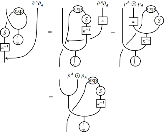
Figure 5: Proof for the first step in Eq. (171).

7 Expectation values of position or momentum

In this chapter, we consider the expectation values of the operators for momentum and position. We calculate these expectation values for solutions to the free $q$-deformed Schrödinger equations [cf. Eqs. (81) and (103) in Chap. 4].

We require that the solutions to the free $q$-deformed Schrödinger equations are subject to the following normalization condition:

$$1=\frac{1}{2}\int\text{d}_{q}^{3}x\left(\phi_{L}^{\ast}(\mathbf{x},t)\circledast\phi_{R}(\mathbf{x},t)+\phi_{L}(\mathbf{x},t)\circledast\phi_{R}^{\ast}(\mathbf{x},t)\right).$$ (172)

This condition is equivalent to

$$1=\frac{1}{2}\int\text{d}_{q}^{3}\hskip 0.72229ptp\left((c^{\ast})_{\mathbf{p}}\circledast c_{\hskip 0.72229pt\mathbf{p}}+c^{\hskip 0.72229pt\mathbf{p}}\circledast(c^{\ast})^{\mathbf{p}}\right).$$ (173)

You can see this by inserting the expressions of Eqs. (132) and (133) into Eq. (172) and proceeding in the following manner:

$$\int\text{d}_{q}^{3}x\,\phi_{L}^{\ast}(\mathbf{x},t)\circledast\phi_{R}(\mathbf{x},t)=$$

$$\qquad=\int\text{d}_{q}^{3}p\int\text{d}_{q}^{3}p^{\prime}(c^{\ast})_{\mathbf{p}}\circledast\int\text{d}_{q}^{3}x\,(u^{\ast})_{\mathbf{p}}(\mathbf{x},t)\circledast u_{\hskip 0.72229pt\mathbf{p}^{\prime}}(\mathbf{x},t)\circledast c_{\hskip 0.72229pt\mathbf{p}^{\prime}}$$

$$\qquad=\int\text{d}_{q}^{3}p\int\text{d}_{q}^{3}p^{\prime}(c^{\ast})_{\mathbf{p}}\circledast\operatorname*{vol}\nolimits^{-1}\delta_{q}^{\hskip 0.72229pt3}((\ominus\hskip 0.72229pt\kappa^{-1}\mathbf{p)}\oplus\mathbf{p}^{\hskip 0.72229pt\prime})\circledast c_{\hskip 0.72229pt\mathbf{p}^{\prime}}$$

$$\qquad=\int\text{d}_{q}^{3}p\,(c^{\ast})_{\mathbf{p}}\circledast c_{\hskip 0.72229pt\mathbf{p}}.$$ (174)

Note that the last two steps of the above calculation follow from Eqs. (118) and (117) of Chap. 5.

We continue with the expectation value of the momentum operator. We determine this expectation value in position space as well as in momentum space:

$$\langle P^{A}\rangle_{\phi} =\frac{1}{2}\int\text{d}_{q}^{3}x\left(\phi_{L}^{\ast}(\mathbf{x},t)\circledast\text{i}^{-1}\partial^{A}\triangleright\phi_{R}(\mathbf{x},t)+\phi_{L}(\mathbf{x},t)\circledast\text{i}^{-1}\partial^{A}\,\bar{\triangleright}\,\phi_{R}^{\ast}(\mathbf{x},t)\right)$$

$$=\frac{1}{2}\int\text{d}_{q}^{3}p\left((c^{\ast})_{\mathbf{p}}\circledast p^{A}\circledast c_{\hskip 0.72229pt\mathbf{p}}+c^{\hskip 0.72229pt\mathbf{p}}\circledast p^{A}\circledast(c^{\ast})^{\mathbf{p}}\right).$$ (175)

To obtain the expression in momentum space from that in position space, we proceed as follows:

$$\int\text{d}_{q}^{3}x\,\phi_{L}^{\ast}(\mathbf{x},t)\circledast\text{i}^{-1}\partial^{A}\triangleright\phi_{R}(\mathbf{x},t)=$$

$$\qquad=\int\text{d}_{q}^{3}p\int\text{d}_{q}^{3}p^{\prime}(c^{\ast})_{\mathbf{p}}\circledast\int\text{d}_{q}^{3}x\,(u^{\ast})_{\mathbf{p}}(\mathbf{x},t)\circledast u_{\hskip 0.72229pt\mathbf{p}^{\prime}}(\mathbf{x},t)\circledast p^{A}\circledast c_{\hskip 0.72229pt\mathbf{p}^{\prime}}$$

$$\qquad=\int\text{d}_{q}^{3}p\int\text{d}_{q}^{3}p^{\prime}(c^{\ast})_{\mathbf{p}}\circledast\operatorname*{vol}\nolimits^{-1}\delta_{q}^{\hskip 0.72229pt3}((\ominus\hskip 0.72229pt\kappa^{-1}\mathbf{p)}\oplus\mathbf{p}^{\hskip 0.72229pt\prime})\circledast p^{A}\circledast c_{\hskip 0.72229pt\mathbf{p}^{\prime}}$$

$$\qquad=\int\text{d}_{q}^{3}p\,(c^{\ast})_{\mathbf{p}}\circledast p^{A}\circledast c_{\hskip 0.72229pt\mathbf{p}}.$$ (176)

In the first step of the above calculation, we used the series expansion in terms of $q$-deformed plane waves [see Eq. (132) in the previous chapter] and applied the eigenvalue equations for $q$-deformed plane waves [see Eq. (82) in Chap. 4]:

$$\text{i}^{-1}\partial^{A}\triangleright\phi_{R}(\mathbf{x},t) =\int\text{d}_{q}^{3}p\,\text{i}^{-1}\partial^{A}\triangleright u_{\hskip 0.72229pt\mathbf{p}}(\mathbf{x},t)\circledast c_{\hskip 0.72229pt\mathbf{p}}$$

$$=\int\text{d}_{q}^{3}p\,u_{\hskip 0.72229pt\mathbf{p}}(\mathbf{x},t)\circledast p^{A}\circledast c_{\hskip 0.72229pt\mathbf{p}}.$$ (177)

The further steps in Eq. (176) correspond to those in Eq. (174).

The expectation value of the momentum operator behaves as follows under conjugation:

$$\overline{\langle P^{A}\rangle_{\phi}}=\langle P_{A}\rangle_{\phi}.$$ (178)

This identity follows from the last expression in Eq. (175) if we take into account Eq. (128) of Chap. 5 as well as the conjugation properties of momentum coordinates, $q$-integral, and star product [cf. Eq. (22) in Chap. 2.1 and Eq. (47) in Chap. 2.2]:

$$\overline{\int\text{d}_{q}^{3}p\,(c^{\ast})_{\mathbf{p}}\circledast p^{A}\circledast c_{\hskip 0.72229pt\mathbf{p}}}=\int\text{d}_{q}^{3}p\,c^{\hskip 0.72229pt\mathbf{p}}\circledast p_{A}\circledast(c^{\ast})^{\mathbf{p}}.$$ (179)

We can also write down expressions for the expectation value of the position operator. Concretely, we have

$$\langle X^{A}\rangle_{\phi} =\frac{1}{2}\int\text{d}_{q}^{3}x\left(\phi_{L}^{\ast}(\mathbf{x},t)\circledast x^{A}\circledast\phi_{R}(\mathbf{x},t)+\phi_{L}(\mathbf{x},t)\circledast x^{A}\circledast\phi_{R}^{\ast}(\mathbf{x},t)\right)$$

$$=\frac{1}{2}\int\text{d}_{q}^{3}p\left((c^{\ast})_{\mathbf{p}}(t)\circledast\text{i}\partial_{p}^{A}\,\bar{\triangleright}\,c_{\hskip 0.72229pt\mathbf{p}}(t)+c^{\hskip 0.72229pt\mathbf{p}}(t)\circledast\text{i}\partial_{p}^{A}\triangleright(c^{\ast})^{\mathbf{p}}(t)\right)$$ (180)

with

$$c_{\hskip 0.72229pt\mathbf{p}}(t) =\exp\left(-\frac{\text{i}t\hskip 0.72229pt\mathbf{p}^{2}}{2\hskip 0.72229ptm}\right)\circledast c_{\hskip 0.72229pt\mathbf{p}}, (c^{\ast})_{\mathbf{p}}(t) =(c^{\ast})_{\mathbf{p}}\circledast\exp\left(\frac{\text{i}t\hskip 0.72229pt\mathbf{p}^{2}}{2\hskip 0.72229ptm}\right),$$

$$c^{\hskip 0.72229pt\mathbf{p}}(t) =c^{\hskip 0.72229pt\mathbf{p}}\circledast\exp\left(\frac{\text{i}t\hskip 0.72229pt\mathbf{p}^{2}}{2\hskip 0.72229ptm}\right), (c^{\ast})^{\mathbf{p}}(t) =\exp\left(-\frac{\text{i}t\hskip 0.72229pt\mathbf{p}^{2}}{2\hskip 0.72229ptm}\right)\circledast(c^{\ast})^{\mathbf{p}}.$$ (181)

To derive the last expression in Eq. (180) from that in position space, we use the series expansion in terms of $q$-deformed plane waves together with the eigenvalue equations

$$x^{A}\circledast\exp_{q}(\mathbf{x}|\text{i}\mathbf{p}) =\exp_{q}(\mathbf{x}|\text{i}\mathbf{p})\,\bar{\triangleleft}\,\partial_{p}^{A}\text{i},$$

$$\text{i}\partial_{p}^{A}\triangleright\exp_{q}(\text{i}^{-1}\mathbf{p}|\mathbf{x}) =\exp_{q}(\text{i}^{-1}\mathbf{p}|\mathbf{x})\circledast x^{A},$$ (182)

and

$$\exp_{q}^{\ast}(\text{i}\mathbf{p}|\mathbf{x})\circledast x^{A} =\text{i}\partial_{p}^{A}\,\bar{\triangleright}\,\exp_{q}^{\ast}(\text{i}\mathbf{p}|\mathbf{x}),$$

$$\exp_{q}^{\ast}(\mathbf{x}|\text{i}^{-1}\mathbf{p})\triangleleft\partial_{p}^{A}\text{i} =x^{A}\circledast\exp_{q}^{\ast}(\mathbf{x}|\text{i}^{-1}\mathbf{p}).$$ (183)

So, we can proceed similarly as in Eq. (176):

$$\int\text{d}_{q}^{3}x\,\phi_{L}^{\ast}(\mathbf{x},t)\circledast x^{A}\circledast\phi_{R}(\mathbf{x},t)=$$

$$\qquad=\int\text{d}_{q}^{3}p\int\text{d}_{q}^{3}p^{\prime}(c^{\ast})_{\mathbf{p}}(t)\circledast\int\text{d}_{q}^{3}x\,\text{i}\partial_{p}^{A}\,\bar{\triangleright}\,(u^{\ast})_{\mathbf{p}}(\mathbf{x},t)\circledast u_{\hskip 0.72229pt\mathbf{p}^{\prime}}(\mathbf{x},t)\circledast c_{\hskip 0.72229pt\mathbf{p}^{\prime}}(t)$$

$$\qquad=\int\text{d}_{q}^{3}p\,(c^{\ast})_{\mathbf{p}}(t)\circledast\text{i}\partial_{p}^{A}\,\bar{\triangleright}\,\operatorname*{vol}\nolimits^{-1}\int\text{d}_{q}^{3}p^{\prime}\delta_{q}^{\hskip 0.72229pt3}((\ominus\hskip 0.72229pt\kappa^{-1}\mathbf{p)}\oplus\mathbf{p}^{\hskip 0.72229pt\prime})\circledast c_{\hskip 0.72229pt\mathbf{p}^{\prime}}(t)$$

$$\qquad=\int\text{d}_{q}^{3}p\,(c^{\ast})_{\mathbf{p}}(t)\circledast\text{i}\partial_{p}^{A}\,\bar{\triangleright}\,c_{\hskip 0.72229pt\mathbf{p}}(t).$$ (184)

For the sake of completeness, we note that the expectation value $\langle X^{A}\rangle_{\phi}$ behaves under conjugation as follows:

$$\overline{\langle X^{A}\rangle_{\phi}}=\langle X_{A}\rangle_{\phi}.$$ (185)

This identity follows from the expression for $\langle X^{A}\rangle_{\phi}$ in position space if we take into account Eq. (104) in Chap. 4 as well as the conjugation properties of spatial coordinates, $q$-integral, and star product.

Also note that the expectation value $\langle X^{A}\rangle_{\phi}$ is usually not time-independent, unlike the expectation value $\langle P^{A}\rangle_{\phi}$. You can see this from the expressions for $\langle X^{A}\rangle_{\phi}$ and $\langle P^{A}\rangle_{\phi}$ in momentum space [cf. Eqs. (175) and (180)].

References

- [1] C. A. Mead. Observable consequences of fundamental-length hypotheses. Phys. Rev., 143:990–1005, 1966.
- [2] L. J. Garay. Quantum gravity and minimum length. Int. J. Phys. A, 10:145–165, 1995.
- [3] H. Snyder. Quantized space-time. Phys. Rev., 71:38–41, 1947.
- [4] S. Doplicher, K. Fredenhagen, and J. E. Roberts. Space-time quantization induced by classical gravity. Phys. Lett. B, 331:39–44, 1994.
- [5] C.-S. Chu and P.-M. Ho. Noncommutative open string and D-brane. Nucl. Phys. B, 550:151–168, 1999. arXiv:hep-th/9812219.
- [6] V. Schomerus. D-branes and deformation quantization. JHEP, 06:30–42, 1999. arXiv:hep-th/9903205.
- [7] J. M. Grimstrup and R. Wulkenhaar. Quantisation of -expanded non-commutative QED. Eur. Phys. J. C, 26(1):139–151, 2002. arXiv:hep-th/0205153.
- [8] J. Lukierski, H. Ruegg, A. Nowicki, and V. N. Tolstoi. -Deformation of Poincaré algebra. Phys. Lett. B, 264:331–338, 1991.
- [9] S. Majid and H. Ruegg. Bicrossproduct structure of -Poincaré group and noncommutative geometry. Phys. Lett. B, 334:348–354, 1994. arXiv:hep-th/9405107.
- [10] L. D. Faddeev, N. Yu. Reshetikhin, and L. A. Takhtajan. Quantization of Lie groups and Lie algebras. Leningrad Math. J., 1:193–225, 1990.
- [11] J. E. Moyal. Quantum mechanics as a statistical theory. Proc. Cambridge Philos. Soc., 45:99–124, 1949.
- [12] G. Carnovale. On the braided Fourier transform in the -dimensional quantum space. J. Math. Phys., 40:5972–5997, 1999. arXiv:math/9810011.
- [13] H. Wachter. Analysis on -deformed quantum spaces. Int. J. Mod. Phys. A, 22:95–164, 2007. arXiv:math-ph/0604028.
- [14] H. Wachter. Momentum and position representations for the -deformed euclidean space. 2019. arXiv:math-ph/1910.02283.
- [15] H. Wachter. Quantum dynamics on the three-dimensional -deformed euclidean space. 2020. arXiv:math-ph/2004.05444.
- [16] A. Lorek, W. Weich, and J. Wess. Non-commutative Euclidean and Minkowski structures. Z. Phys. C, 76:375–386, 1997.
- [17] F. Bayen, M. Flato, C. Fronsdal, A. Lichnerowicz, and D. Sternheimer. Deformation theory and quantization. 1. Deformations of symplectic structures. Ann. Phys., 111:61–110, 1978.
- [18] M. Kontsevich. Deformation quantization of Poisson manifolds, I. arXiv:q-alg/9709040, 1997.
- [19] J. Madore, S. Schraml, P. Schupp, and J. Wess. Gauge theory on noncommutative spaces. Eur. Phys. J. C, 16:161–167, 2000. arXiv:hep-th/0001203.
- [20] H. Wachter and M. Wohlgenannt. -Products on quantum spaces. Eur. Phys. J. C, 23:761–767, 2002. arXiv:hep-th/0103120.
- [21] F. N. Jackson. -Difference equations. Amer. J. Math., 32:305–314, 1910.
- [22] U. Carow-Watamura, M. Schlieker, and S. Watamura. SOq()-covariant differential calculus on quantum space and quantum deformation of Schroedinger equation. Z. Phys. C, 49:439–446, 1991.
- [23] J. Wess and B. Zumino. Covariant differential calculus on the quantum hyperplane. Nucl. Phys. Proc. Suppl. B, 18:302–312, 1991.
- [24] C. Bauer and H. Wachter. Operator representations on quantum spaces. Eur. Phys. J. C, 31:261–275, 2003. arXiv:math-ph/0201023.
- [25] H. Wachter. -Integration on quantum spaces. Eur. Phys. J. C, 32:281–297, 2004. arXiv:hep-th/0206083.
- [26] F. N. Jackson. On -definite integrals. Quart. J. Pure and Appl. Math., 41:193–203, 1910.
- [27] C. Jambor. Non-Commutative Analysis on Quantum Spaces. Dissertation, Fak. f. Phys., LMU München, 2004.
- [28] A. Kempf and S. Majid. Algebraic -integration and Fourier theory on quantum and braided spaces. J. Math. Phys., 35:6802–6837, 1994. arXiv:hep-th/9402037.
- [29] S. Majid. Free braided differential calculus, braided binomial theorem and the braided exponential map. J. Math. Phys., 34:4843–4856, 1993.
- [30] A. Schirrmacher. Generalized -exponentials related to orthogonal quantum groups and Fourier transformations of noncommutative spaces. J. Math. Phys., 36:1531–1546, 1995.
- [31] H. Wachter. -Exponentials on quantum spaces. Eur. Phys. J. C, 37:370–389, 2004. arXiv:hep-th/040113.
- [32] C. Chryssomalakos and B. Zumino. Translations, integrals and Fourier transforms in the quantum plan. In A. Ali, J. Ellis, and S. Randjbar-Daemi, editors, Salamfestschrift, Proccedings of the Conference on Highlights of Particle and Condensed Matter Physics, ICTP, Trieste/Italy, 1993.
- [33] H. Wachter. Elemente einer -Analysis für physikalisch relevante Quantenräume. Dissertation, Fak. f. Phys., LMU München, 2004.
- [34] S. Majid. Foundations of Quantum Group Theory. University Press, Cambridge/UK, 1995.
- [35] S. Majid. A Quantum Groups Primer. University Press, Cambridge/UK, 2002.
- [36] V. Kac and P. Cheung. Quantum Calculus. Universitext. Springer, New York - Berlin - Heidelberg, 2002.