MESA: Boost Ensemble Imbalanced Learning with MEta-SAmpler

Abstract

Imbalanced learning (IL), i.e., learning unbiased models from class-imbalanced data, is a challenging problem. Typical IL methods including resampling and reweighting were designed based on some heuristic assumptions. They often suffer from unstable performance, poor applicability, and high computational cost in complex tasks where their assumptions do not hold. In this paper, we introduce a novel ensemble IL framework named Mesa. It adaptively resamples the training set in iterations to get multiple classifiers and forms a cascade ensemble model. Mesa directly learns the sampling strategy from data to optimize the final metric beyond following random heuristics. Moreover, unlike prevailing meta-learning-based IL solutions, we decouple the model-training and meta-training in Mesa by independently train the meta-sampler over task-agnostic meta-data. This makes Mesa generally applicable to most of the existing learning models and the meta-sampler can be efficiently applied to new tasks. Extensive experiments on both synthetic and real-world tasks demonstrate the effectiveness, robustness, and transferability of Mesa. Our code is available at https://github.com/ZhiningLiu1998/mesa.

1 Introduction

Class imbalance, due to the naturally-skewed class distributions, has been widely observed in many real-world applications such as click prediction, fraud detection, and medical diagnosis [13, 15, 21]. Canonical classification algorithms usually induce the bias, i.e., perform well in terms of global accuracy but poorly on the minority class, in solving class imbalance problems. However, the minority class commonly yields higher interests from both learning and practical perspectives [18, 19].

Typical imbalanced learning (IL) algorithms attempt to eliminate the bias through data resampling [6, 16, 17, 26, 35] or reweighting [30, 33, 40] in the learning process. More recently, ensemble learning is incorporated to reduce the variance introduced by resampling or reweighting and has achieved satisfactory performance [23]. In practice, however, all these methods have been observed to suffer from three major limitations: (I) unstable performance due to the sensitivity to outliers, (II) poor applicability because of the prerequisite of domain experts to hand-craft the cost matrix, and (III) high cost of computing the distance between instances.

Regardless the computational issue, we attribute the unsatisfactory performance of traditional IL methods to the validity of heuristic assumptions made on training data. For instance, some methods [7, 12, 32, 39] assume instances with higher training errors are more informative for learning. However, misclassification may be caused by outliers, and error reinforcement arises in this case with the above assumption. Another widely used assumption is that generating synthetic samples around minority instances helps with learning [7, 8, 46]. This assumption only holds when the minority data is well clustered and sufficiently discriminative. If the training data is extremely imbalanced or with many corrupted labels, the minority class would be poorly represented and lack a clear structure. In this case, working under this assumption severely jeopardizes the performance.

Henceforth, it is much more desired to develop an adaptive IL framework that is capable of handling complex real-world tasks without intuitive assumptions. Inspired by the recent developments in meta-learning [25], we propose to achieve the meta-learning mechanism in ensemble imbalanced learning (EIL) framework. In fact, some preliminary efforts [37, 38, 41] have investigated the potential of applying meta-learning to IL problems. Nonetheless, these works have limited capability of generalization because of the model-dependent optimization process. Their meta-learners are confined to be co-optimized with a single DNN, which greatly limits their application to other learning models (e.g., tree-based models) as well as deployment into the more powerful EIL framework.

In this paper, we propose a generic EIL framework Mesa that automatically learns its strategy, i.e., the meta-sampler, from data towards optimizing imbalanced classification. The main idea is to model a meta-sampler that serves as an adaptive under-sampling solution embedded in the iterative ensemble training process. In each iteration, it takes the current state of ensemble training (i.e., the classification error distribution on both the training and validation sets) as its input. Based on this, the meta-sampler selects a subset to train a new base classifier and then adds it to the ensemble, a new state can thus be obtained. We expect the meta-sampler to maximize the final generalization performance by learning from such interactions. To this end, we use reinforcement learning (RL) to solve the non-differentiable optimization problem of the meta-sampler. To summarize, this paper makes the following contributions. (I) We propose Mesa, a generic EIL framework that demonstrates superior performance by automatically learning an adaptive under-sampling strategy from data. (II) We carry out a preliminary exploration of extracting and using cross-task meta-information in EIL systems. The usage of such meta-information gives the meta-sampler cross-task transferability. A pretrained meta-sampler can be directly applied to new tasks, thereby greatly reducing the computational cost brought about by meta-training. (III) Unlike prevailing methods whose meta-learners were designed to be co-optimized with a specific learning model (i.e, DNN) during training, we decoupled the model-training and meta-training process in Mesa. This makes our framework generally applicable to most of the statistical and non-statistical learning models (e.g., decision tree, Naïve Bayes, k-nearest neighbor classifier).

2 Related Work

Fernández et al. [1], Guo et al. [15], and He et al. [18, 19] provided systematic reviews of algorithms and applications of imbalanced learning. In this paper, we focus on binary imbalanced classification problem, which is one of the most widely studied problem setting [15, 23] in imbalanced learning. Such a problem extensively exists in practical applications, e.g., fraud detection (fraud vs. normal), medical diagnosis (sick vs. healthy), and cybersecurity (intrusion vs. user connection). We mainly review existing works on this problem as follows.

Resampling Resampling methods focus on modifying the training set to balance the class distribution (i.e., over/under-sampling [6, 16, 17, 35, 42]) or filter noise (i.e., cleaning resampling [26, 45]). Random resampling usually leads to severe information loss or overfishing, hence many advanced methods explore distance information to guide their sampling process [15]. However, calculating the distance between instances is computationally expensive on large-scale datasets, and such strategies may even fail to work when the data does not fit their assumptions.

Reweighting Reweighting methods assign different weights to different instances to alleviate a classifier’s bias towards majority groups (e.g., [5, 12, 31, 33]). Many recent reweighting methods such as FocalLoss [30] and GHM [28] are specifically designed for DNN loss function engineering. Class-level reweighting such as cost-sensitive learning [33] is more versatile but requires a cost matrix given by domain experts beforehand, which is usually infeasible in practice.

Ensemble Methods. Ensemble imbalanced learning (EIL) is known to effectively improve typical IL solutions by combining the outputs of multiple classifiers (e.g., [7, 32, 34, 39, 46]). These EIL approaches prove to be highly competitive [23] and thus gain increasing popularity [15] in IL. However, most of the them are straight combinations of a resampling/reweighting solution and an ensemble learning framework, e.g., Smote [6]+AdaBoost [12]=SmoteBoost [7]. Consequently, although EIL techniques effectively lower the variance introduced by resampling/reweighting, these methods still suffer from unsatisfactory performance due to their heuristic-based designs.

Meta-learning Methods. Inspired by recent meta-learning developments [11, 25], there are some studies that adapt meta-learning to solve IL problem. Typical methods include Learning to Teach [48] that learns a dynamic loss function, MentorNet [22] that learns a mini-batch curriculum, and L2RW [38]/Meta-Weight-Net [41] that learn an implicit/explicit data weighting function. Nonetheless, all these methods are confined to be co-optimized with a DNN by gradient descent. As the success of deep learning relies on the massive training data, mainly from the well-structured data domain like computer vision and natural language processing, the applications of these methods to other learning models (e.g., tree-based models and their ensemble variants like gradient boosting machine) in traditional classification tasks (e.g., small/unstructured/tabular data) are highly constrained.

We present a comprehensive comparison of existing IL solutions for binary imbalanced classification problem with our Mesa in Table 1. Compared with other methods, Mesa aims to learn a resampling strategy directly from data. It is able to perform quick and adaptive resampling as no distance computing, domain knowledge, or related heuristics are involved in the resampling process.

Table 1: Comparisons of Mesa with existing imbalanced learning methods, note that $\mathcal{|N|}\gg\mathcal{|P|}$.

Category*	Representative(s)	Sample	Distance-based	Domain kno-	Robust to noi-	Requirements
		efficiency	resampling cost	wledge free?	ses/outliers?
RW	[31], [5]	$\mathcal{O(|P|+|N|)}$	✗	✗	✓✗	cost matrix set by domain experts
US	[35], [42]	$\mathcal{O}(2|\mathcal{P}|)$	$\mathcal{O}(|\mathcal{P}|)$	✓	✗	well-defined distance metric
OS	[6], [17]	$\mathcal{O}(2|\mathcal{N}|)$	$\mathcal{O}(|\mathcal{P}|)$	✓	✗	well-defined distance metric
CS	[47], [44]	$\mathcal{O(|P|+|N|)}$	$\mathcal{O}(|\mathcal{P}|\cdot|\mathcal{N}|)$	✓	✓	well-defined distance metric
OS+CS	[4], [3]	$\mathcal{O}(2|\mathcal{N}|)$	$\mathcal{O}(|\mathcal{P}|\cdot|\mathcal{N}|)$	✓	✓	well-defined distance metric
IE+RW	[12], [43]	$\mathcal{O}(k(\mathcal{|P|+|N|}))$	✗	✗	✗	cost matrix set by domain experts
PE+US	[2], [32]	$\mathcal{O}(2k|\mathcal{P}|)$	✗	✓	✓	-
PE+OS	[46]	$\mathcal{O}(2k|\mathcal{N}|)$	$\mathcal{O}(2k|\mathcal{P}|)$	✓	✓	well-defined distance metric
IE+RW+US	[39]	$\mathcal{O}(2k|\mathcal{P}|)$	✗	✓	✗	-
IE+RW+OS	[7]	$\mathcal{O}(2k|\mathcal{N}|)$	$\mathcal{O}(2k|\mathcal{P}|)$	✓	✗	well-defined distance metric
ML	[41], [38], [48]	$\mathcal{O(|P|+|N|)}$	✗	✓✗	✓	co-optimized with DNN only
IE+ML	MESA(ours)	$\mathcal{O}(2k|\mathcal{P}|)$	✗	✓	✓	independent meta-training

• reweighting (RW), under-sampling (US), over-sampling (OS), cleaning-sampling (CS), iterative ensemble (IE), parallel ensemble (PE), meta-learning (ML).

3 The proposed Mesa framework

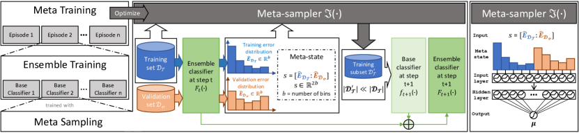
Figure 1: Overview of the proposed Mesa Framework. Best viewed in color.

In order to take advantage of both ensemble learning and meta-learning, we propose a novel EIL framework named Mesa that works with a meta-sampler. As shown in Fig. 1, Mesa consists of three parts: meta-sampling as well as ensemble training to build ensemble classifiers, and meta-training to optimize the meta-sampler. We will describe them respectively in this section.

Specifically, Mesa is designed to: (I) perform resampling based on meta-information to further boost the performance of ensemble classifiers; (II) decouple model-training and meta-training for general applicability to different classifiers; (III) train the meta-sampler over task-agnostic meta-data for cross-task transferability and reducing meta-training cost on new tasks.

Notations. Let $\mathcal{X}:\mathbb{R}^{d}$ be the input feature space and $\mathcal{Y}:\{0,1\}$ be the label space. An instance is represented by $(x,y)$, where $x\in\mathcal{X}$, $y\in\mathcal{Y}$. Without loss of generality, we always assume that the minority class is positive. Given an imbalanced dataset $\mathcal{D}:\{(x_{1},y_{1}),(x_{2},y_{2}),\cdots,(x_{n},y_{n})\}$, the minority set is $\mathcal{P}:\{(x,y)\ |\ y=1,(x,y)\in\mathcal{D}\}$ and the majority set is $\mathcal{N}:\{(x,y)\ |\ y=0,(x,y)\in\mathcal{D}\}$. For highly imbalanced data we have $|\mathcal{N}|\gg|\mathcal{P}|$. We use $f:x\to[0,1]$ to denote a single classifier and $F_{k}:x\to[0,1]$ to denote an ensemble classifier that is formed by $k$ base classifiers. We use $\mathcal{D}_{\tau}$ and $\mathcal{D}_{v}$ to represent the training set and validation set, respectively.

Meta-state. As mentioned before, we expect to find a task-agnostic representation that can provide the meta-sampler with the information of the ensemble training process. Motivated by the concept of “gradient/hardness distribution” from [28, 34], we introduce the histogram distribution of the training and validation errors as the meta-state of the ensemble training system.

Formally, given an data instance $(x,y)$ and an ensemble classifier $F_{t}(\cdot)$, the classification error $e$ is defined as the absolute difference between the predicted probability of $x$ being positive and the ground truth label $y$, i.e., $|F_{t}(x)-y|$. Suppose the error distribution on dataset $\mathcal{D}$ is $E_{\mathcal{D}}$, then the error distribution approximated by histogram is given by a vector $\widehat{E}_{\mathcal{D}}\in\mathbb{R}^{b}$, where $b$ is the number of bins in the histogram. Specifically, the $i$-th component of vector $\widehat{E}_{\mathcal{D}}$ can be computed as follows:

$$\widehat{E}_{\mathcal{D}}^{i}=\frac{|\{(x,y)\ |\ \frac{i-1}{b}\leq abs(F_{t}(x)-y)<\frac{i}{b}\ ,(x,y)\in\mathcal{D}\}|}{|\mathcal{D}|},1\leq i\leq b.$$ (1)

After concatenating the error distribution vectors on training and validation set, we have the meta-state:

$$s=[\widehat{E}_{\mathcal{D}_{\tau}}:\widehat{E}_{\mathcal{D}_{v}}]\in\mathbb{R}^{2b}.$$ (2)

Intuitively, the histogram error distribution $\widehat{E}_{\mathcal{D}}$ shows how well the given classifier fits the dataset $\mathcal{D}$. When $b=2$, it reports the accuracy score in $\widehat{E}_{\mathcal{D}}^{1}$ and misclassification rate in $\widehat{E}_{\mathcal{D}}^{2}$ (classification threshold is 0.5). With $b>2$, it shows the distribution of “easy” samples (with errors close to 0) and “hard” samples (with errors close to 1) in finer granularity, thus contains more information to guide the resampling process. Moreover, since we consider both the training and validation set, the meta-state also provides the meta-sampler with information about bias/variance of the current ensemble model and thus supporting its decision. We show some illustrative examples in Fig. 2.

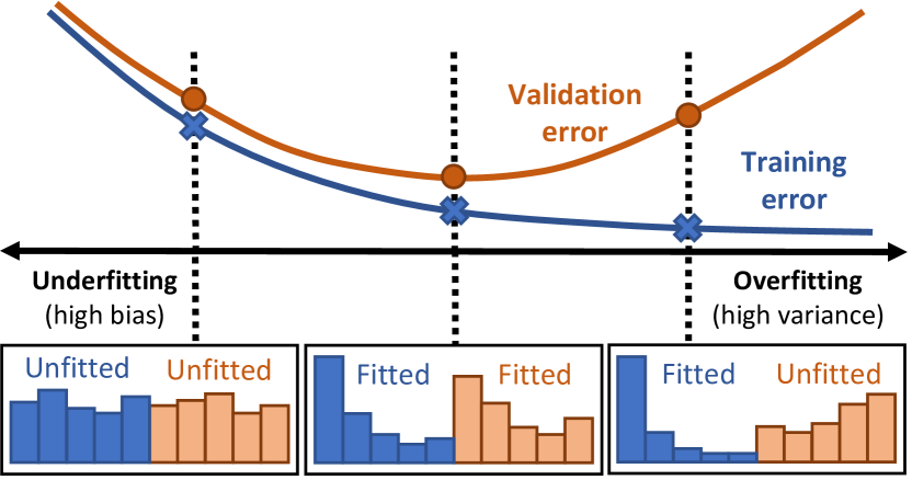
Figure 2: Some examples of different meta-states ($s=[\widehat{E}_{\mathcal{D}_{\tau}}:\widehat{E}_{\mathcal{D}_{v}}]$) and their corresponding ensemble training states. The meta-state reflects how well the current classifier fits on the training set, and how well it generalizes to unseen validation data. Note that such representation is independent of properties of the specific task (e.g., dataset size, feature space) thus can be used to support the meta-sampler to perform adaptive resampling across different tasks.

Meta Sampling. Making instance-level decisions by using a complex meta-sampler (e.g., set a large output layer or use recurrent neural network) is extremely time-consuming as the complexity of a single update $C_{u}$ is $\mathcal{O}(|\mathcal{D}|)$. Besides, complex model architecture also brings extra memory cost and hardship in optimization. To make Mesa more concise and efficient, we use a Gaussian function trick to simplify the meta-sampling process and the sampler itself, reducing $C_{u}$ from $\mathcal{O}(|\mathcal{D}|)$ to $\mathcal{O}(1)$.

Specifically, let $\Im$ denote the meta-sampler, it outputs a scalar $\mu\in[0,1]$ based on the input meta-state $s$, i.e., $\mu\thicksim\Im(\mu|s)$. We then apply a Gaussian function $g_{\mu,\sigma}(x)$ over each instance’s classification error to decide its (unnormalized) sampling weight, where $g_{\mu,\sigma}(x)$ is defined as:

$$g_{\mu,\sigma}(x)=\frac{1}{\sigma\sqrt{2\pi}}e^{-\frac{1}{2}(\frac{x-\mu}{\sigma})^{2}}.$$ (3)

Note that in Eq. 3, $e$ is the Euler’s number, $\mu\in[0,1]$ is given by the meta-sampler and $\sigma$ is a hyper-parameter. Please refer to Section C.2 for discussions and guidelines about our hyper-parameter setting. The above meta-sampling procedure $\texttt{Sample}(~{}\cdot~{};F,\mu,\sigma)$ is summarized in Algorithm 1.

Algorithm 1 $\text{\tt Sample}(\mathcal{D}_{\tau};F,\mu,\sigma)$

1:$\mathcal{D}_{\tau}$, $F$, $\mu$, $\sigma$

2:Initialization: derive majority set $\mathcal{P}_{\tau}$ and minority set $\mathcal{N}_{\tau}$ from $\mathcal{D}_{\tau}$ 

3:Assign each $(x_{i},y_{i})$ in $\mathcal{N}_{\tau}$ with weight:

$$w_{i}=\frac{g_{\mu,\sigma}(|F(x_{i})-y_{i}|)}{\sum_{(x_{j},y_{j})\in\mathcal{N}_{\tau}}g_{\mu,\sigma}(|F(x_{j})-y_{j}|)}$$

4:Sample majority subset $\mathcal{N}_{\tau}^{{}^{\prime}}$ from $\mathcal{N}_{\tau}$ w.r.t. sampling weights $w$, where $|\mathcal{N}_{\tau}^{{}^{\prime}}|=|\mathcal{P}_{\tau}|$ 

5:return balanced subset $\mathcal{D}_{\tau}^{{}^{\prime}}=\mathcal{N}_{\tau}^{{}^{\prime}}\cup\mathcal{P}_{\tau}$

Algorithm 2 Ensemble training in Mesa

1:$\mathcal{D}_{\tau}$, $\mathcal{D}_{v}$, $\Im$, $\sigma$, $f$, $b$, $k$

2:train $f_{1}(x)$ with random balanced subset 

3:for $t$=1 to $k-1$ do

4:     $F_{t}(x)=\frac{1}{t}\sum_{i=1}^{t}f_{i}(x)$ 

5:     compute $\widehat{E}_{\mathcal{D}_{\tau}}$ and $\widehat{E}_{\mathcal{D}_{v}}$ by Eq. 1 

6:     $s_{t}=[\widehat{E}_{\mathcal{D}_{\tau}}:\widehat{E}_{\mathcal{D}_{v}}]$ 

7:     $\mu_{t}\thicksim\Im(\mu_{t}|s_{t})$ 

8:     $\mathcal{D}^{{}^{\prime}}_{t\text{+1},\tau}=\text{\tt Sample}(\mathcal{D}_{\tau};F_{t},\mu_{t},\sigma)$ 

9:     train new classifier $f_{t\text{+1}}(x)$ with $\mathcal{D}^{{}^{\prime}}_{t\text{+1},\tau}$ 

10:return $F_{k}(x)=\frac{1}{k}\sum_{i=1}^{k}f_{i}(x)$

Ensemble Training. Given a meta-sampler $\Im:\mathbb{R}^{2b}\to[0,1]$ and the meta-sampling strategy, we can iteratively train new base classifiers using the dataset sampled by the sampler. At the $t$-th iteration, having the current ensemble $F_{t}(\cdot)$, we can obtain $\widehat{E}_{\mathcal{D}_{\tau}}$, $\widehat{E}_{\mathcal{D}_{v}}$ and meta-state $s_{t}$ by applying Eqs. (1) and (2). Then a new base classifier $f_{t+1}(\cdot)$ is trained with the subset $\mathcal{D}^{{}^{\prime}}_{t+1,\tau}=\texttt{Sample}(\mathcal{D}_{\tau};F_{t},\mu_{t},\sigma)$, where $\mu_{t}\thicksim\Im(\mu_{t}|s_{t})$ and $\mathcal{D}_{\tau}$ is the original training set. Note that $f_{1}(\cdot)$ was trained on a random balanced subset, as there is no trained classifier in the first iteration. See Algorithm 2 for more details.

Algorithm 3 Meta-training in Mesa

1:Initialization: replay memory $\mathcal{M}$ with capacity $N$, network parameters $\psi,\bar{\psi},\theta,$ and $\varphi$

2:for episode = 1 to $M$ do

3:     for each environment step $t$ do

4:         observe $s_{t}$ from $\mathsf{ENV}$ $\triangleright$ line3-5 in Alg. 2 

5:         take action $\mu_{t}\thicksim\Im_{\varphi}(\mu_{t}|s_{t})$ $\triangleright$ line6-8 in Alg. 2 

6:         observe reward $r_{t}=P(F_{t\text{+1}},\mathcal{D}_{v})-P(F_{t},\mathcal{D}_{v})$ and $s_{t+1}$

7:         store transition $\mathcal{M}=\mathcal{M}\cup\{(s_{t},\mu_{t},r_{t},s_{t+1})\}$      

8:     for each gradient step do

9:         update $\psi,\bar{\psi},\theta,$ and $\varphi$ according to [14]      

10:return meta-sampler $\Im$ with parameters $\varphi$

Meta Training. As described above, our meta-sampler $\Im$ is trained to optimize the generalized performance of an ensemble classifier by iteratively selecting its training data. It takes the current state $s$ of the training system as input, and then outputs the parameter $\mu$ of a Gaussian function to decide each instance’s sampling probability. The meta-sampler is expected to learn and adapt its strategy from such state($s$)-action($\mu$)-state(new $s$) interactions. The non-differentiable optimization problem of training $\Im$ can thus be naturally approached via reinforcement learning (RL).

We consider the ensemble training system as the environment ($\mathsf{ENV}$) in the RL setting. The corresponding Markov decision process (MDP) is defined by the tuple ($\mathcal{S},\mathcal{A},p,r$), where the state space $\mathcal{S}:\mathbb{R}^{2b}$ and action space $\mathcal{A}:[0,1]$ is continuous, and the unknown state transition probability $p:\mathcal{S\times S\times A}\to[0,\infty)$ represents the probability density of the next state $s_{t+1}\in\mathcal{S}$ given the current state $s_{t}\in\mathcal{S}$ and action $a_{t}\in\mathcal{A}$. More specifically, in each episode, we iteratively train $k$ base classifiers $f(\cdot)$ and form a cascade ensemble classifier $F_{k}(\cdot)$. In each environment step, $\mathsf{ENV}$ provides the meta-state $s_{t}=[\widehat{E}_{\mathcal{D}_{\tau}}:\widehat{E}_{\mathcal{D}_{v}}]$, and then the action $a_{t}$ is selected by $a_{t}\thicksim\Im(\mu_{t}|s_{t})$, i.e., $a_{t}\Leftrightarrow\mu_{t}$. A new base classifier $f_{t+1}(\cdot)$ is trained using the subset $\mathcal{D}^{{}^{\prime}}_{t+1,\tau}=Sample(\mathcal{D}_{\tau};F_{t},a_{t},\sigma)$. After adding $f_{t+1}(\cdot)$ into the ensemble, the new state $s_{t+1}$ was sampled w.r.t. $s_{t+1}\thicksim p(s_{t+1};s_{t},a_{t})$. Given a performance metric function $P(F,\mathcal{D})\to\mathbb{R}$, the reward $r$ is set to the generalization performance difference of $F$ before and after an update (using the keep-out validation set for unbiased estimation), i.e., $r_{t}=P(F_{t+1},\mathcal{D}_{v})-P(F_{t},\mathcal{D}_{v})$. The optimization goal of the meta-sampler (i.e., the cumulative reward) is thus the generalization performance of the ensemble classifier.

We take advantage of Soft Actor-Critic [14] (Sac), an off-policy actor-critic deep RL algorithm based on the maximum entropy RL framework, to optimize our meta-sampler $\Im$. In our case, we consider a parameterized state value function $V_{\psi}(s_{t})$ and its corresponding target network $V_{\bar{\psi}}(s_{t})$, a soft Q-function $Q_{\theta}(s_{t},a_{t})$, and a tractable policy (meta-sampler) $\Im_{\varphi}(a_{t}|s_{t})$. The parameters of these networks are $\psi,\bar{\psi},\theta,$ and $\varphi$. The rules for updating these parameters are given in the Sac paper [14]. We summarize the meta-training process of $\Im_{\varphi}$ in Algorithm 3.

Complexity analysis. Please refer to Section C.1 for detailed complexity analysis of Mesa alongside with related validating experiments in Fig. 7.

4 Experiments

To thoroughly assess the effectiveness of Mesa, two series of experiments are conducted: one on controlled synthetic toy datasets for visualization and the other on real-world imbalanced datasets to validate Mesa’s performance in practical applications. We also carry out extended experiments on real-world datasets to verify the robustness and cross-task transferability of Mesa.

4.1 Experiment on Synthetic Datasets

Setup Details. We build a series of imbalanced toy datasets corresponding to different levels of underlying class distribution overlapping, as shown in Fig. 3. All the datasets have the same imbalance ratio ($|\mathcal{N}|/|\mathcal{P}|=2,000/200=10$). In this experiment, Mesa is compared with four representative EIL algorithms from 4 major EIL branches (Parallel/Iterative Ensemble + Under/Over-sampling), i.e., SmoteBoost [7], SmoteBagging [46], RusBoost [39], and UnderBagging [2]. All EIL methods are deployed with decision trees as base classifiers with ensemble size of $5$.

Visualization & Analysis. We plot the input datasets and the decision boundaries learned by different EIL algorithms in Fig.fig:visualization, which shows that Mesa achieves the best performance under different situations. We can observe that: all tested methods perform well on the less-overlapped dataset (1st row). Note that random under-sampling discards some important majority samples (e.g., data points at the right end of the “$\cap$”-shaped distribution) and cause information loss. This makes the performance of RusBoost and UnderBagging slightly weaker than their competitors. As overlapping intensifies (2nd row), an increasing amount of noise gains high sample weights during the training process of boosting-based methods, i.e., SmoteBoost and RusBoost, thus resulting in poor classification performance. Bagging-based methods, i.e., SmoteBagging and UnderBagging, are less influenced by noise but they still underperform Mesa. Even on the extremely overlapped dataset (3rd row), Mesa still gives a stable and reasonable decision boundary that fits the underlying distribution. This is because the meta-sampler can adaptively select informative training subsets towards the good prediction performance while being robust to noise/outliers. All the results show the superiority of our Mesa to other traditional EIL baselines in handling the distribution overlapping, noises, and poor minority class representation.

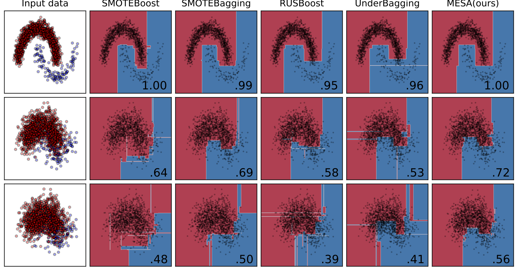
Figure 3: Comparisons of Mesa with 4 representative traditional EIL methods (SmoteBoost [7], SmoteBagging [46], RusBoost [39] and UnderBagging [2]) on 3 toy datasets with different levels of underlying class distribution overlapping (less/mid/highly-overlapped in 1st/2nd/3rd row). The number in the lower right corner of each subfigure represents the AUCPRC score of the corresponding classifier. Best viewed in color.

4.2 Experiment on Real-world Datasets

Setup Details. In order to verify the effectiveness of Mesa in practical applications, we extend the experiments to real-world imbalanced classification tasks from the UCI repository [10] and KDD CUP 2004. To ensure a thorough assessment, these datasets vary widely in their properties, with the imbalance ratio (IR) ranging from 9.1:1 to 111:1, dataset sizes ranging from 531 to 145,751, and number of features ranging from 6 to 617 (Please see Table 7 in Section B for detailed information). For each dataset, we keep-out the 20% validation set and report the result of 4-fold stratified cross-validation (i.e., 60%/20%/20% training/validation/test split). The performance is evaluated using the area under the precision-recall curve (AUCPRC), which is an unbiased and more comprehensive metric for class-imbalanced tasks compared to other metrics such as F-score, ROC, and accuracy [9].

Table 2: Comparisons of Mesa with other representative resampling methods.

Category	Method	Protein Homo. (IR=111)					#Training	Resampling
		KNN	GNB	DT	AdaBoost	GBM	Samples	Time (s)
No resampling	-	0.466	0.742	0.531	0.778	0.796	87,450	-
Under-sampling	RandomUS	0.146	0.738	0.071	0.698	0.756	1,554	0.068
	NearMiss [35]	0.009	0.012	0.012	0.400	0.266	1,554	3.949
Cleaing-sampling	Clean [26]	0.469	0.744	0.488	0.781	0.811	86,196	117.739
	ENN [47]	0.460	0.744	0.532	0.789	0.817	86,770	120.046
	TomekLink [45]	0.466	0.743	0.524	0.778	0.791	87,368	90.633
	AllKNN [44]	0.459	0.744	0.542	0.789	0.816	86,725	327.110
	OSS [24]	0.466	0.743	0.536	0.778	0.789	87,146	92.234
Over-sampling	RandomOS	0.335	0.706	0.505	0.736	0.733	173,346	0.098
	Smote [6]	0.189	0.753	0.304	0.700	0.719	173,346	0.576
	ADASYN [17]	0.171	0.679	0.315	0.717	0.693	173,366	2.855
	BorderSmote [16]	0.327	0.743	0.448	0.795	0.711	173,346	2.751
Over-sampling + Cleaning	SmoteENN [4]	0.156	0.750	0.308	0.711	0.750	169,797	156.641
	SmoteTomek [3]	0.185	0.749	0.292	0.782	0.703	173,346	116.401
Meta-sampler	Mesa (OURS, $k$=10)	0.585	0.804	0.832	0.849	0.855	1,554$\times$10	0.235$\times$10

Comparison with Resampling Imbalanced Learning (IL) Methods. We first compare Mesa with resampling techniques, which have been widely used in practice for preprocessing imbalanced data [15]. We select 12 representative methods from 4 major branches of resampling-based IL, i.e, under/over/cleaning-sampling and over-sampling with cleaning-sampling post-process. We test all methods on the challenging highly-imbalanced (IR=111) Protein Homo. task to check their efficiency and effectiveness. Five different classifiers, i.e., K-nearest neighbor (KNN), Gaussian Naïve Bayes (GNB), decision tree (DT), adaptive boosting (AdaBoost), and gradient boosting machine (GBM), were used to collaborate with different resampling approaches. We also record the number of samples used for model training and the time used to perform resampling.

Table 2 details the experiment results. We show that by learning an adaptive resampling strategy, Mesa outperforms other traditional data resampling methods by a large margin while only using a small number of training instances. In such a highly imbalanced dataset, the minority class is poorly represented and lacks a clear structure. Thus over-sampling methods that rely on relations between minority objects (like Smote) may deteriorate the classification performance, even though they generate and use a huge number of synthetic samples for training. On the other hand, under-sampling methods drop most of the samples according to their rules and results in significant information loss and poor performance. Cleaning-sampling methods aim to remove noise from the dataset, but the resampling time is considerably high and the improvement is trivial.

Table 3: Comparisons of Mesa with other representative under-sampling-based EIL methods.

Method	Optical Digits (IR=9.1)			Spectrometer (IR=11)			ISOLET (IR=12)			Mammography (IR=42)
	$k$=5	$k$=10	$k$=20	$k$=5	$k$=10	$k$=20	$k$=5	$k$=10	$k$=20	$k$=5	$k$=10	$k$=20
RusBoost [39]	0.883	0.946	0.958	0.686	0.784	0.786	0.696	0.770	0.789	0.348	0.511	0.588
UnderBagging [2]	0.876	0.927	0.954	0.610	0.689	0.743	0.688	0.768	0.812	0.307	0.401	0.483
SPE [34]	0.906	0.959	0.969	0.688	0.777	0.803	0.755	0.841	0.895	0.413	0.559	0.664
Cascade [32]	0.862	0.932	0.958	0.599	0.754	0.789	0.684	0.819	0.891	0.404	0.575	0.670
Mesa (OURS)	0.929	0.968	0.980	0.723	0.803	0.845	0.787	0.877	0.921	0.515	0.644	0.705

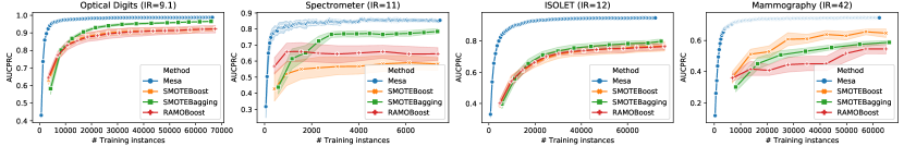
Figure 4: Comparisons of Mesa with other representative over-sampling-based EIL methods.

Comparison with Ensemble Imbalanced Learning (EIL) Methods. We further compare Mesa with 7 representative EIL methods on four real-world imbalanced classification tasks. The baselines include 4 under-sampling based EIL methods, i.e., RusBoost [39], UnderBagging [2], SPE [34], Cascade [32], and 3 over-sampling-based EIL methods, i.e., SmoteBoost [7], SmoteBagging [46] and RamoBoost [8]. We use the decision tree as the base learner for all EIL methods following the settings of most of the previous works [15].

We report the AUCPRC score of various USB-EIL methods with different ensemble sizes ($k$=5, 10, 20) in Table 3. The results show that Mesa achieves competitive performance on various real-world tasks. For the baseline methods, we can observe that RusBoost and UnderBagging suffer from information loss as random under-sampling may discard samples with important information, and such effect is more apparent on highly imbalanced task. In comparison, the improved sampling strategies of SPE and Cascade enable them to achieve relatively better performance but still underperform Mesa. Moreover, as Mesa provides an adaptive resampler that makes the ensemble training converge faster and better, its advantage is particularly evident when using small ensemble in the highly-imbalanced task. On the Mammography dataset (IR=42), compared with the second-best score, Mesa achieved 24.70%/12.00%/5.22% performance gain when $k$=5/10/20, respectively.

We further compare Mesa with 3 OSB-EIL methods. As summarized in Table 1, OSB-EIL methods typically use much more (1-2$\times$IR times) data to train each base learner than their under-sampling-based competitors, including Mesa. Thus it is unfair to directly compare Mesa with over-sampling-based baselines with the same ensemble size. Therefore, we plot the performance curve with regard to the number of instances used in ensemble training, as shown in Fig. 4.

It can be observed that our method Mesa consistently outperforms over-sampling-based methods, especially on highly imbalanced/high-dimensional tasks (e.g., ISOLET with 617 features, Mammo. with IR=42). Mesa also shows high sample efficiency and faster convergence speed. Compared with the baselines, it only requires a few training instances to converge to a strong ensemble classifier. Mesa also has a more stable training process. The OSB-EIL methods perform resampling by analyzing and reinforcing the structure of minority class data. When the dataset is small or highly-imbalanced, the minority class is usually under-represented and lacks a clear structure. The performance of these OSB-EIL methods thus becomes unstable under such circumstances.

Table 4: Cross-task transferability of the meta-sampler.

	Mammography (IR=42, 11,183 instances)				Protein Homo. (IR=111, 145,751 instances)
	$k$=10	$\Delta$	$k$=20	$\Delta$	$k$=10	$\Delta$	$k$=20	$\Delta$
100%	0.644$\pm$0.028	baseline	0.705$\pm$0.015	baseline	0.840$\pm$0.009	baseline	0.874$\pm$0.008	baseline
50% subset	0.642$\pm$0.032	-0.30%	0.702$\pm$0.017	-0.43%	0.839$\pm$0.009	-0.12%	0.872$\pm$0.009	-0.23%
10% subset	0.640$\pm$0.031	-0.62%	0.700$\pm$0.017	-0.71%	0.839$\pm$0.008	-0.10%	0.871$\pm$0.006	-0.34%
Optical Digits	0.637$\pm$0.029	-1.09%	0.701$\pm$0.015	-0.57%	0.839$\pm$0.006	-0.12%	0.870$\pm$0.006	-0.46%
Spectrometer	0.641$\pm$0.025	-0.54%	0.697$\pm$0.021	-1.13%	0.836$\pm$0.009	-0.48%	0.870$\pm$0.006	-0.46%

Cross-task Transferability of the Meta-sampler. One important feature of Mesa is its cross-task transferability. As the meta-sampler is trained on task-agnostic meta-data, it is not task-bounded and is directly applicable to new tasks. This provides Mesa with better scalability as one can directly use a pre-trained meta-sampler in new tasks thus greatly reduce the meta-training cost. To validate this, we use Mammography and Protein Homo. as two larger and highly-imbalanced meta-test tasks, then consider five meta-training tasks including the original task (baseline), two sub-tasks with 50%/10% of the original training set, and two small tasks Optical Digits and Spectrometer.

Table 4 reports the detailed results. We can observe that the transferred meta-samplers generalize well on meta-test tasks. Scaling down the number of meta-training instances has a minor effect on the obtained meta-sampler, especially when the original task has a sufficient number of training samples (e.g., for Protein Homo., reducing the meta-training set to 10% subset only results in -0.10%/-0.34% $\Delta$ when $k$=10/20). Moreover, the meta-sampler that trained on a small task also demonstrates noticeably satisfactory performance (superior to other baselines) on new, larger, and even heterogeneous tasks, which validates the generality of the proposed Mesa framework. Please refer to Section A for a comprehensive cross/sub-task transferability test and other additional experimental results.

5 Conclusion

We propose a novel imbalanced learning framework Mesa. It contains a meta-sampler that adaptively selects training data to learn effective cascade ensemble classifiers from imbalanced data. Rather than following random heuristics, Mesa directly optimizes its sampling strategy for better generalization performance. Compared with prevailing meta-learning IL solutions that are limited to be co-optimized with DNNs, Mesa is a generic framework capable of working with various learning models. Our meta-sampler is trained over task-agnostic meta-data and thus can be transferred to new tasks, which greatly reduces the meta-training cost. Empirical results show that Mesa achieves superior performance on various tasks with high sample efficiency. In future work, we plan to explore the potential of meta-knowledge-driven ensemble learning in the long-tail multi-classification problem.

6 Statement of the Potential Broader Impact

In this work, we study the problem of imbalanced learning (IL), which is a common problem related to machine learning and data mining. Such a problem widely exists in many real-world application domains such as finance, security, biomedical engineering, industrial manufacturing, and information technology [15]. IL methods, including the proposed Mesa framework in this paper, aim to fix the bias of learning models introduced by skewed training class distribution. We believe that proper usage of these techniques will lead us to a better society. For example, better IL techniques can detect phishing websites/fraud transactions to protect people’s property, and help doctors diagnose rare diseases/develop new medicines to save people’s lives. With that being said, we are also aware that using these techniques improperly can cause negative impacts, as misclassification is inevitable in most of the learning systems. In particular, we note that when deploying IL systems in medical-related domains, misclassification (e.g., failure to identify a patient) could lead to medical malpractice. In such domains, these techniques should be used as auxiliary systems, e.g., when performing diagnosis, we can adjust the classification threshold to achieve higher recall and use the predicted probability as a reference for the doctor’s diagnosis. While there are some risks with IL research, as we mentioned above, we believe that with proper usage and monitoring, the negative impact of misclassification could be minimized and IL techniques can help people live a better life.

Appendix A Additional Results

A.1 Cross-task and sub-task transferability of the meta-sampler

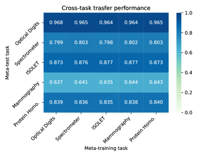
(a) Cross-task transfer performance.

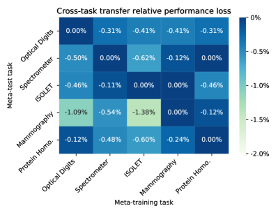
(b) Cross-task transfer performance loss.

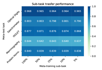
(c) Sub-task transfer performance.

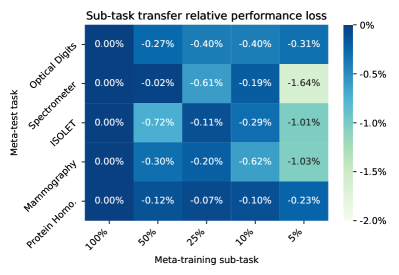
(d) Sub-task transfer performance loss.

Figure 5: Cross/Sub-task transfer performance loss of Mesa.

In addition to results reported in Table 4, we conduct further experiments on all five tasks to test the cross-task transferability of the meta-sampler. The results are presented in Fig. 5 (with $k$=10). For the cross-task transfer experiment, we meta-train the meta-sampler on each task separately, then apply it on other unseen meta-test tasks. As shown in Fig. 5(b), in all 20 heterogenous training-test task pairs, 18/20 of them manage to have less than 1% performance loss. On the other hand, in the sub-task transfer experiment, for each task, we meta-train the meta-sampler on 100%/50%/25%/10%/5% subset, then apply it back to the original full dataset. Again Mesa shows robust performance, in all 20 subset transfer experiments, 17/20 of them manage to have less than 1% performance loss. The effect of reducing the meta-training set scale is more significant in small datasets. The largest performance loss (-1.64%) is reported in {5%, Spectrometer} setting, which is the smallest dataset with only 531 instances. For large datasets, scaling down the meta-training set greatly reduces the number of instances as well as meta-training costs, while only brought about minor performance loss, e.g., -0.23% loss in {5%, Protein Homo.}.

A.2 Robustness to corrupted labels.

In practice, the collected training dataset may contain corrupted labels. Typical examples include data labeled by crowdsourcing systems or search engines [20, 29]. The negative impact brought by noise is particularly prominent on skewed datasets that inherently have an unclear minority data structure. In this experiment, Mammography and Protein Homo. tasks are used to test the robustness of different EIL methods on highly-imbalanced datasets. We simulate real-world corrupted labels by introducing flip noise. Specifically, flip the labels of $r_{\text{noise}}$% (i.e., $|\mathcal{P}|\cdot r_{\text{noise}}$) minority samples in the training set from 1 to 0. Accordingly, an equal number of majority samples are flipped from 0 to 1. We thereby get a noisy dataset with the same IR. For each dataset, we test the USB-EIL methods with $k=10$ trained on the 0%/10%/25%/40% noisy training sets.

The results are summarized in Table 5, which shows that Mesa consistently outperforms other baselines under different levels of label noise. The meta-sampler $\Im$ in Mesa can efficiently prevent the ensemble classifier from overfitting noise as it is optimized for generalized performance, while the performance of other methods decrease rapidly as the noise level increases. Compared with the second-best baselines, Mesa achieves 12.00%/14.44%/10.29%/7.22% (Mammography) and 2.56%/3.20%/6.92%/9.72% (Protein Homo.) performance gain when $r_{\text{noise}}$=0%/10%/25%/40%.

Table 5: Generalized performances on real-world imbalanced datasets with varying label noise ratios.

	Mammography (IR=42, 11,183 instances)				Protein Homo. (IR=111, 145,751 instances)
	$r_{\text{noise}}$=0%	$r_{\text{noise}}$=10%	$r_{\text{noise}}$=25%	$r_{\text{noise}}$=40%	$r_{\text{noise}}$=0%	$r_{\text{noise}}$=10%	$r_{\text{noise}}$=25%	$r_{\text{noise}}$=40%
RusBoost [39]	0.511	0.448	0.435	0.374	0.738	0.691	0.628	0.502
UnderBagging [2]	0.401	0.401	0.375	0.324	0.632	0.629	0.629	0.617
SPE [34]	0.559	0.476	0.405	0.345	0.819	0.775	0.688	0.580
Cascade [32]	0.575	0.540	0.447	0.357	0.805	0.781	0.708	0.594
Mesa (OURS)	0.644	0.618	0.493	0.401	0.840	0.806	0.757	0.677

A.3 Cross-task meta-training

In the meta-training process of Mesa, collecting transitions is independent of the updates of the meta-sampler. This enables us to simultaneously collect meta-data from multiple datasets and thus to co-optimize the meta-sampler over these tasks. There may be some states that can rarely be observed in a specific dataset, in such case, parallelly collecting transitions from multiple datasets also helps our meta-sampler exploring the state space and learns a better policy. Moreover, as previously discussed, a converged meta-sampler can be directly applied to new and even heterogeneous tasks. Hence by cross-task meta-training, we can obtain a meta-sampler that not only works well on training tasks but is also able to boost Mesa’s performance on unseen (meta-test) tasks. To verify this, we follow the setup in section 4 using two small tasks for cross-task meta-training and two large tasks for the meta-test. We plot the generalized performance on all the four tasks during the cross-task meta-training process, as shown in Fig 6. The performance scores of other representative EIL methods from Table 3 are also included. Note that we only plot the two best performing baselines in each subfigure for better visualization.

At the very start of meta-training, the meta-sampler $\Im$ is initialized with random weights. Its performance is relatively poor at this point. But as meta-training progresses, $\Im$ adjusts its sampling strategy to maximize the expected generalized performance. After 50-60 training episodes, Mesa surpasses the best performing baseline method and continued to improve. Finally, we get a meta-sampler that is able to undertake adaptive under-sampling and thereby outperform other EIL methods on all meta-training and meta-test tasks.

= 2pt

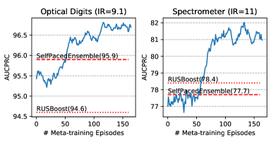
(a) Performance in meta-training tasks

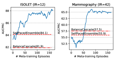
(b) Performance in meta-test tasks

Figure 6: Visualization of Mesa’s cross-task meta-training process (slide mean window = 50).

A.4 Ablation study

To assess the importance of Gaussian function weighted meta-sampling and meta-sampler respectively, we carry out ablation experiments on 4 real-world datasets. They are Optical Digits, Spectrometer, ISOLET, and Mammography with increasing IR (9.1/11/12/42). Our experiments shown in Table 6 indicate that Mesa significantly improves performance, especially when using small ensembles on highly imbalanced datasets.

Table 6: Ablation study of Mesa on 4 real-world datasets. Random policy refers to using randomly initialized meta-sampler to perform meta-sampling. $k$ represents the ensemble size. $\Delta$ is the relative performance loss (%) compared to Mesa policy.

Dataset	Method	$k=5$	$\Delta$	$k=10$	$\Delta$	$k=20$	$\Delta$
Optical Digits	Mesa policy	0.929	baseline	0.968	baseline	0.980	baseline
	Random policy	0.904	-1.61%	0.959	-0.93%	0.975	-0.51%
	Random sampling	0.876	-5.71%	0.927	-4.24%	0.954	-2.65%
Spectrometer	Mesa policy	0.723	baseline	0.803	baseline	0.845	baseline
	Random policy	0.685	-5.26%	0.774	-3.61%	0.800	-5.33%
	Random sampling	0.610	-15.63%	0.692	-13.82%	0.755	-10.65%
ISOLET	Mesa policy	0.787	baseline	0.877	baseline	0.921	baseline
	Random policy	0.748	-4.96%	0.849	-3.19%	0.891	-3.26%
	Random sampling	0.688	-12.58%	0.768	-12.43%	0.812	-11.83%
Mammography	Mesa policy	0.515	baseline	0.644	baseline	0.705	baseline
	Random policy	0.405	-21.36%	0.568	-11.80%	0.662	-6.10%
	Random sampling	0.307	-40.39%	0.401	-37.73%	0.483	-31.49%

Appendix B Implementation Details

Table 7: Description of the real-world imbalanced datasets.

Dataset	Repository	Target	Imbalance Ratio	#Samples	#Features
Optical Digits	UCI	target: 8	9.1:1	5,620	64
Spectrometer	UCI	target: $\geq 44$	11:1	531	93
ISOLET	UCI	target: A, B	12:1	7,797	617
Mammography	UCI	target: minority	42:1	11,183	6
Protein Homo.	KDDCUP 2004	target: minority	111:1	145,751	74

Datasets. All datasets used in this paper are publicly available, and are summarized in Table 7. One can fetch these datasets using the imblearn.dataset API of the imbalanced-learn [27] Python package. For each dataset, we keep-out the 20% validation set and report the result of 4-fold stratified cross-validation (i.e., 60%/20%/20% train/valid/test split). We also perform class-wise split to ensure that the imbalanced ratio of the training, validation, and test sets after splitting is the same.

Base classifiers. All used base classifiers (i.e., K-nearest neighbor classifier, Gaussian native bayes, decision tree, adaptive boosting, gradient boosting machine) are implemented using scikit-learn [36] Python package. For the ensemble models (i.e., adaptive boosting and gradient boosting), we set the n_estimators = 10. All other parameters use the default setting specified by the scikit-learn package.

Implementation of baseline methods. All baseline resampling IL methods (RandomUS, NearMiss [35], Clean [26], ENN [47], TomekLink [45], AllKNN [44], OSS [24], Smote [6], ADASYN [17], BorderSmote [16], SmoteENN [4], and SmoteTomek [3]) are implemented in imbalanced-learn Python package [27]. We directly use their implementation and default hyper-parameters in our experiments. We use open-source code for implementation of baseline ensemble imbalanced learning (EIL) methods (RusBoost [39], UnderBagging [2], Cascade [32], SPE [34], SmoteBoost [7], SmoteBagging [46], and RamoBoost [8]). The hyper-parameters of these baseline EIL methods are reported in Table 10.

Implementation of Mesa. Mesa is implemented with PyTorch. The empirical results reported in the paper use hyper-parameters in Tables 10 and 10 for the meta-training of Mesa. We open-sourced our Mesa implementation at Github with a jupyter notebook file that allows you to quickly (I) conduct a comparative experiment, (II) visualize the meta-training process of Mesa, and (III) visualize the experimental results. Please check the repository for more information.

Table 8: Hyper-parameters of EIL baselines.

Method	Hyper-parameter	Value
RusBoost [39]	n_samples	100
	min_ratio	1.0
	with_replacement	True
	learning_rate	1.0
	algorithm	SAMME.R
SmoteBoost [7]	n_samples	100
	k_neighbors	5
	learning_rate	1.0
	algorithm	SAMME.R
RamoBoost [8]	n_samples	100
	k_neighbors_1	5
	k_neighbors_2	5
	alpha	0.3
	learning_rate	1.0
	algorithm	SAMME.R
UnderBagging [2]	- - -	- - -
SmoteBagging [46]	k_neighbors	5
BalanceCascade [32]	- - -	- - -
SelfPacedEnsemble [34]	hardness_func	cross entropy
	k_bins	10

Table 9: Hyper-parameters of SAC [14].

Hyper-parameter	Value
Policy type	Gaussian
Reward discount factor ($\gamma$)	0.99
Smoothing coefficient ($\tau$)	0.01
Temperature parameter ($\alpha$)	0.1
Learning rate	1e-3
Learning rate decay steps	10
Learning rate decay ratio	0.99
Mini-batch size	64
Replay memory size	1e3
Steps of gradient updates	1e3
Steps of random actions	5e2

Table 10: Hyper-parameters of Mesa.

Hyper-parameter	Value
Meta-state size	10
Gaussian function parameter $\sigma$	0.2

The actor policy network of meta-sampler is a multi-layer perceptron with one hidden layer containing 50 nodes. Its architecture is thus {state_size, 50, 1}. The corresponding (target) critic Q-network is also an MLP but with two hidden layers. As it takes both state and action as input, its architecture is thus {state_size+1, 50, 50, 1}. Each hidden node is with ReLU activation function, and the output of the policy network is with the tanh activation function, to guarantee the output located in the interval of $[0,1]$. As a general network training trick, we employ the Adam optimizer to optimize the policy and critic networks.

Table 11: Performance of different policy network architectures.

Network Architecture	Optical Digits Task
	$k$=5	$k$=10	$k$=20
{10, 50, 1}	0.929$\pm$0.015	0.968$\pm$0.007	0.980$\pm$0.003
{10, 100, 1}	0.930$\pm$0.014	0.966$\pm$0.007	0.979$\pm$0.004
{10, 200, 1}	0.922$\pm$0.018	0.964$\pm$0.008	0.978$\pm$0.005
{10, 25, 25, 1}	0.928$\pm$0.014	0.966$\pm$0.007	0.980$\pm$0.004
{10, 50, 50, 1}	0.929$\pm$0.017	0.967$\pm$0.008	0.978$\pm$0.004
{10, 100, 100, 1}	0.926$\pm$0.015	0.966$\pm$0.010	0.979$\pm$0.006
{10, 10, 10, 10, 1}	0.924$\pm$0.013	0.964$\pm$0.007	0.977$\pm$0.004
{10, 25, 25, 25, 1}	0.924$\pm$0.016	0.966$\pm$0.006	0.978$\pm$0.002
{10, 50, 50, 50, 1}	0.926$\pm$0.006	0.965$\pm$0.006	0.979$\pm$0.005

We test different network architecture settings in experiments. Table 11 depicts some representative results under 9 different policy network structures, with different depths and widths. It can be observed that varying MLP settings have no substantial effects on the final result. We hence prefer to use the simple and shallow one.

Appendix C Discussion

C.1 Complexity analysis of the proposed framework

Our Mesa framework can be roughly regarded as an under-sampling-based ensemble imbalanced learning (EIL) framework (Algorithm 2) with an additional sampler meta-training process (Algorithm 3).

Ensemble training. Given an imbalanced dataset $\mathcal{D}$ with majority set $\mathcal{N}$ and minority set $\mathcal{P}$, where $|\mathcal{N}|\gg|\mathcal{P}|$. Suppose that the cost of training a base classifier $f(\cdot)$ with $N$ training instances is $C_{f\text{train}}(N)$. As Mesa performs strictly balanced under-sampling to train each classifier, we have

$$\text{Cost of $k$-classifier ensemble training}:k\cdot C_{f\text{train}}(2|\mathcal{P}|)$$

In comparison, the cost is $k\cdot C_{f\text{train}}(|\mathcal{N}|+|\mathcal{P}|)$ for reweighting-based EIL methods (e.g., AdaBoost) and around $k\cdot C_{f\text{train}}(2|\mathcal{N}|)$ for over-sampling-based EIL methods (e.g., SmoteBagging).

Meta-training. Let’s denote the cost of performing a single gradient update step of the meta-sampler $\Im$ as $C_{\Im\text{update}}$, this cost mainly depends on the choice of the policy/critic network architecture. It is barely influenced by other factors such as the dataset size in ensemble training. In our Mesa implementation, we do $n_{\text{random}}$ steps for collecting transitions with random actions before start updating $\Im$, and $n_{\text{update}}$ steps for collecting online transitions and perform gradient updates to $\Im$. Then we have

$$\text{Cost of meta-training}:(n_{\text{random}}+n_{\text{update}})\cdot C_{f\text{train}}(2|\mathcal{P}|)+n_{\text{update}}\cdot C_{\Im\text{update}}$$

As mentioned before, the meta-training cost can be effectively reduced by scaling down the meta-training dataset (i.e., reducing $|\mathcal{P}|$). This can be achieved by using a subset of the original data in meta-training. One can also directly use a meta-sampler pre-trained on other (smaller) dataset to avoid the meta-training phase when applying Mesa to new tasks. Both ways should only bring minor performance loss, as reported in Fig. 5.

Note that, reducing the number of meta-training instances only influences the $C_{f\text{train}}(\cdot)$ term. Therefore, the larger the $C_{f\text{train}}(2|\mathcal{P}|)/C_{\Im\text{update}}$, the higher the acceleration ratio brought by shrinking the meta-training set. We also show some results in Fig. 7 to demonstrate such influence. The decision tree classifier we used has no max depth limitation, thus its training cost is higher when dealing with high-dimensional data. We thus choose three tasks with different numbers of features for the test, they are Mammography/Protein Homo./ISOLET with 6/74/617 features. It can be observed that the acceleration effect is slightly weaker for the low-dimensional Mammography task, as the cost of training base classifier is small compared with the cost of updating meta-sampler. On the other hand, for those high-dimensional tasks (i.e., ISOLET and Protein Homo.), shrinking the meta-training set greatly reduces the cost of meta-sampler training as we expect.

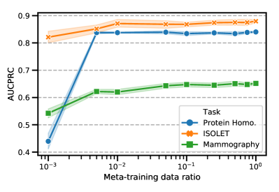
(a) Sub-task transfer performance.

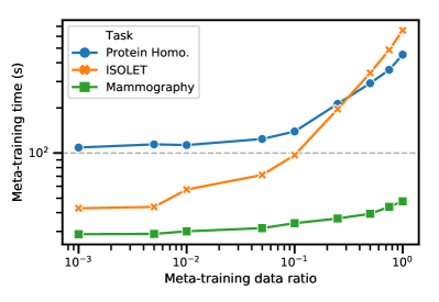
(b) Sub-task meta-training time.

Figure 7: The influence of scaling down the meta-training set.

C.2 Guideline of selecting Mesa hyper-parameters

The meta-state size $b$ determines how detailed our error distribution approximation is (i.e., the number of bins in the histogram). Thus setting a small meta-state size may lead to poor performance. Increasing it to a large value (e.g., $\geq$20) brings greater computational cost but only trivial performance increment. We recommend setting the meta state size to be 10. One can try a bigger meta-state when working on larger datasets.

The Gaussian function parameter $\sigma$ determines how to execute meta-sampling in Mesa. Specifically, given an action $\mu$, we expect the meta-sampling selects those instances with error values close to $\mu$. Besides, the meta-sampling is also responsible for providing diversity, which is an important characteristic in classifiers combination. A small $\sigma$ can guarantee to select examples with small errors around $\mu$, but this would result in subsets that lack diversity. For example, in the late iterations of ensemble training, most of the data instances have stable error values, and meta-sampling with small $\sigma$ will always return the same training set for a specific $\mu$. This is detrimental to further improve the ensemble classifier. Setting a large $\sigma$ will “flatten ” the Gaussian function, more instances with different errors are likely to be selected and thus bring more diversity. However, when $\sigma\to\infty$, the meta-sampling turns into uniform random under-sampling that makes no sense for meta-training. We also note that although one can expand the policy to automatically determine $\sigma$, it requires additional computational cost and the benefit is very limited. More importantly, selecting inappropriate $\sigma$ will interfere with the quality of collected transitions, causing an unstable meta-training process. Therefore, we suggest using $\sigma=0.2$ to balance between these factors.

Appendix D Visualization

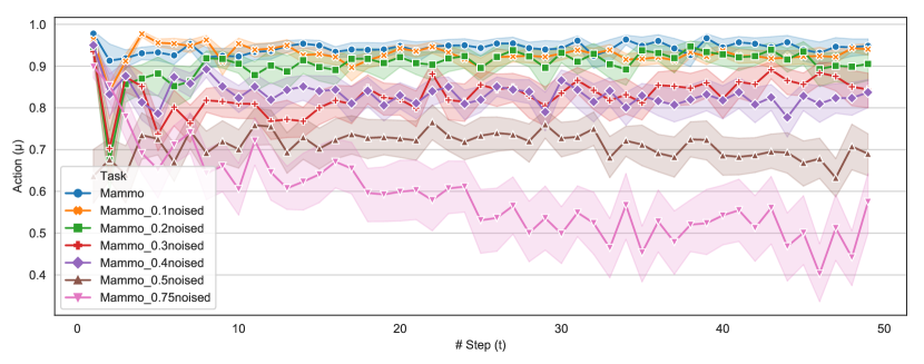
Figure 8: Learned meta-sampler policies on Mammography dataset with varying label noise ratios.

D.1 Visualization of learned meta-sampler policy

We visualize the learned meta-sampler policy under different levels of noises in Fig. 8. It clearly shows that the sampling strategy becomes more conservative as the noise ratio grows. At the very start of ensemble training, there are only a few base learners and thus the ensemble classifier underfits the training set. At this point, the meta-sampler tends to select training instances with larger errors, hence accelerating the fitting process. It continues to use such a strategy on datasets with no/few noises. However, on highly noisy datasets (e.g., with label noise ratio $\geq$ 40%), the meta-sampler prefers to select training instances with relatively lower errors in later iterations as the hard-to-classify instances are likely to be noises/outliers. This effectively prevents the ensemble classifier from overfitting noisy data points.

D.2 Visualization of meta-training process

We visualize the meta-training process in Fig. 9. As the meta-training progress, the classification performance shows consistent improvement in training, validation, and test set in all tasks.

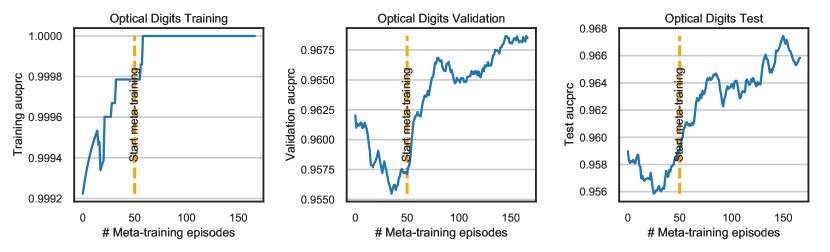
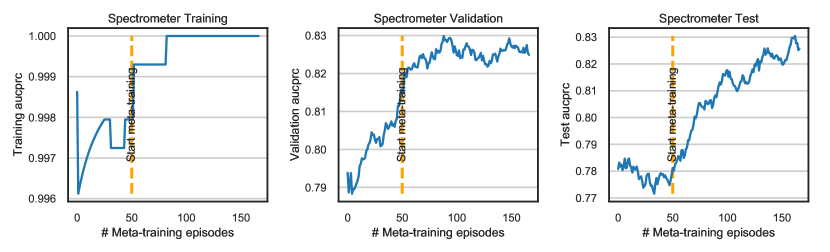
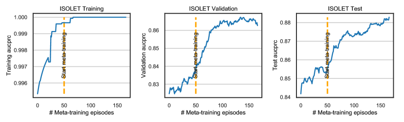
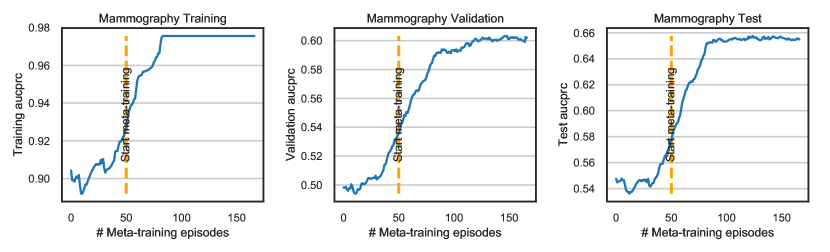
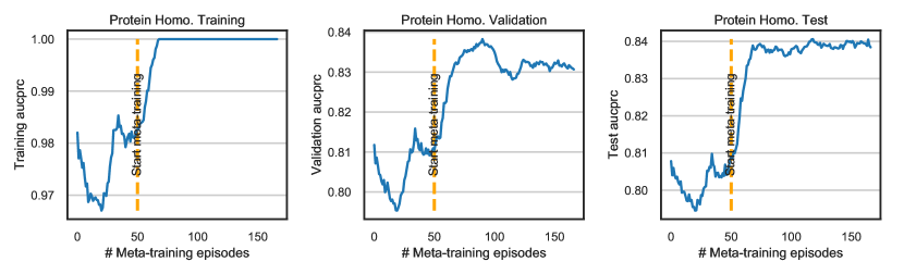
Figure 9: Train/Validation/Test performance during meta-training process (slide mean window=50).

References

- [1] Fernández Alberto, García Salvador, Galar Mikel, Prati Ronaldo C., and Krawczyk Bartosz. Learning from Imbalanced Data Sets. Springer, 2018.
- [2] Ricardo Barandela, Rosa Maria Valdovinos, and José Salvador Sánchez. New applications of ensembles of classifiers. Pattern Analysis & Applications, 6(3):245–256, 2003.
- [3] Gustavo EAPA Batista, Ana LC Bazzan, and Maria Carolina Monard. Balancing training data for automated annotation of keywords: a case study. In WOB, pages 10–18, 2003.
- [4] Gustavo EAPA Batista, Ronaldo C Prati, and Maria Carolina Monard. A study of the behavior of several methods for balancing machine learning training data. ACM SIGKDD explorations newsletter, 6(1):20–29, 2004.
- [5] Xiaoyong Chai, Lin Deng, Qiang Yang, and Charles X Ling. Test-cost sensitive naive bayes classification. In Fourth IEEE International Conference on Data Mining (ICDM’04), pages 51–58. IEEE, 2004.
- [6] Nitesh V Chawla, Kevin W Bowyer, Lawrence O Hall, and W Philip Kegelmeyer. Smote: synthetic minority over-sampling technique. Journal of artificial intelligence research, 16:321–357, 2002.
- [7] Nitesh V Chawla, Aleksandar Lazarevic, Lawrence O Hall, and Kevin W Bowyer. Smoteboost: Improving prediction of the minority class in boosting. In European conference on principles of data mining and knowledge discovery, pages 107–119. Springer, 2003.
- [8] Sheng Chen, Haibo He, and Edwardo A Garcia. Ramoboost: ranked minority oversampling in boosting. IEEE Transactions on Neural Networks, 21(10):1624–1642, 2010.
- [9] Jesse Davis and Mark Goadrich. The relationship between precision-recall and roc curves. In Proceedings of the 23rd international conference on Machine learning, pages 233–240. ACM, 2006.
- [10] Dheeru Dua and Casey Graff. UCI machine learning repository, 2017.
- [11] Chelsea Finn, Pieter Abbeel, and Sergey Levine. Model-agnostic meta-learning for fast adaptation of deep networks. In Proceedings of the 34th International Conference on Machine Learning-Volume 70, pages 1126–1135. JMLR. org, 2017.
- [12] Yoav Freund and Robert E Schapire. A decision-theoretic generalization of on-line learning and an application to boosting. Journal of computer and system sciences, 55(1):119–139, 1997.
- [13] Thore Graepel, Joaquin Quinonero Candela, Thomas Borchert, and Ralf Herbrich. Web-scale bayesian click-through rate prediction for sponsored search advertising in microsoft’s bing search engine. Omnipress, 2010.
- [14] Tuomas Haarnoja, Aurick Zhou, Pieter Abbeel, and Sergey Levine. Soft actor-critic: Off-policy maximum entropy deep reinforcement learning with a stochastic actor. In International Conference on Machine Learning, pages 1861–1870, 2018.
- [15] Guo Haixiang, Li Yijing, Jennifer Shang, Gu Mingyun, Huang Yuanyue, and Gong Bing. Learning from class-imbalanced data: Review of methods and applications. Expert Systems with Applications, 73:220–239, 2017.
- [16] Hui Han, Wen-Yuan Wang, and Bing-Huan Mao. Borderline-smote: a new over-sampling method in imbalanced data sets learning. In International conference on intelligent computing, pages 878–887. Springer, 2005.
- [17] Haibo He, Yang Bai, Edwardo A Garcia, and Shutao Li. Adasyn: Adaptive synthetic sampling approach for imbalanced learning. In 2008 IEEE International Joint Conference on Neural Networks (IEEE World Congress on Computational Intelligence), pages 1322–1328. IEEE, 2008.
- [18] Haibo He and Edwardo A Garcia. Learning from imbalanced data. IEEE Transactions on Knowledge & Data Engineering, (9):1263–1284, 2008.
- [19] Haibo He and Yunqian Ma. Imbalanced learning: foundations, algorithms, and applications. John Wiley & Sons, 2013.
- [20] Dan Hendrycks, Mantas Mazeika, Duncan Wilson, and Kevin Gimpel. Using trusted data to train deep networks on labels corrupted by severe noise. In Advances in neural information processing systems, pages 10456–10465, 2018.
- [21] Nathalie Japkowicz and Shaju Stephen. The class imbalance problem: A systematic study. Intelligent data analysis, 6(5):429–449, 2002.
- [22] Lu Jiang, Zhengyuan Zhou, Thomas Leung, Li-Jia Li, and Li Fei-Fei. Mentornet: Learning data-driven curriculum for very deep neural networks on corrupted labels. arXiv preprint arXiv:1712.05055, 2017.
- [23] Bartosz Krawczyk. Learning from imbalanced data: open challenges and future directions. Progress in Artificial Intelligence, 5(4):221–232, 2016.
- [24] Miroslav Kubat, Stan Matwin, et al. Addressing the curse of imbalanced training sets: one-sided selection. In Icml, volume 97, pages 179–186. Nashville, USA, 1997.
- [25] Brenden M Lake, Ruslan Salakhutdinov, and Joshua B Tenenbaum. Human-level concept learning through probabilistic program induction. Science, 350(6266):1332–1338, 2015.
- [26] Jorma Laurikkala. Improving identification of difficult small classes by balancing class distribution. In Conference on Artificial Intelligence in Medicine in Europe, pages 63–66. Springer, 2001.
- [27] Guillaume Lemaître, Fernando Nogueira, and Christos K. Aridas. Imbalanced-learn: A python toolbox to tackle the curse of imbalanced datasets in machine learning. Journal of Machine Learning Research, 18(17):1–5, 2017.
- [28] Buyu Li, Yu Liu, and Xiaogang Wang. Gradient harmonized single-stage detector. In Proceedings of the AAAI Conference on Artificial Intelligence, volume 33, pages 8577–8584, 2019.
- [29] Yuncheng Li, Jianchao Yang, Yale Song, Liangliang Cao, Jiebo Luo, and Li-Jia Li. Learning from noisy labels with distillation. In Proceedings of the IEEE International Conference on Computer Vision, pages 1910–1918, 2017.
- [30] Tsung-Yi Lin, Priya Goyal, Ross Girshick, Kaiming He, and Piotr Dollár. Focal loss for dense object detection. In Proceedings of the IEEE international conference on computer vision, pages 2980–2988, 2017.
- [31] Charles X Ling, Qiang Yang, Jianning Wang, and Shichao Zhang. Decision trees with minimal costs. In Proceedings of the twenty-first international conference on Machine learning, page 69. ACM, 2004.
- [32] Xu-Ying Liu, Jianxin Wu, and Zhi-Hua Zhou. Exploratory undersampling for class-imbalance learning. IEEE Transactions on Systems, Man, and Cybernetics, Part B (Cybernetics), 39(2):539–550, 2009.
- [33] Xu-Ying Liu and Zhi-Hua Zhou. The influence of class imbalance on cost-sensitive learning: An empirical study. In Sixth International Conference on Data Mining (ICDM’06), pages 970–974. IEEE, 2006.
- [34] Zhining Liu, Wei Cao, Zhifeng Gao, Jiang Bian, Hechang Chen, Yi Chang, and Tie-Yan Liu. Self-paced ensemble for highly imbalanced massive data classification. In 2020 IEEE 36th International Conference on Data Engineering (ICDE). IEEE, 2020.
- [35] Inderjeet Mani and I Zhang. knn approach to unbalanced data distributions: a case study involving information extraction. In Proceedings of workshop on learning from imbalanced datasets, volume 126, 2003.
- [36] Fabian Pedregosa, Gaël Varoquaux, Alexandre Gramfort, Vincent Michel, Bertrand Thirion, Olivier Grisel, Mathieu Blondel, Peter Prettenhofer, Ron Weiss, Vincent Dubourg, et al. Scikit-learn: Machine learning in python. Journal of machine learning research, 12(Oct):2825–2830, 2011.
- [37] Minlong Peng, Qi Zhang, Xiaoyu Xing, Tao Gui, Xuanjing Huang, Yu-Gang Jiang, Keyu Ding, and Zhigang Chen. Trainable undersampling for class-imbalance learning. 2019.
- [38] Mengye Ren, Wenyuan Zeng, Bin Yang, and Raquel Urtasun. Learning to reweight examples for robust deep learning. In International Conference on Machine Learning, pages 4334–4343, 2018.
- [39] Chris Seiffert, Taghi M Khoshgoftaar, Jason Van Hulse, and Amri Napolitano. Rusboost: A hybrid approach to alleviating class imbalance. IEEE Transactions on Systems, Man, and Cybernetics-Part A: Systems and Humans, 40(1):185–197, 2010.
- [40] Abhinav Shrivastava, Abhinav Gupta, and Ross Girshick. Training region-based object detectors with online hard example mining. In Proceedings of the IEEE conference on computer vision and pattern recognition, pages 761–769, 2016.
- [41] Jun Shu, Qi Xie, Lixuan Yi, Qian Zhao, Sanping Zhou, Zongben Xu, and Deyu Meng. Meta-weight-net: Learning an explicit mapping for sample weighting. In NeurIPS, 2019.
- [42] Michael R Smith, Tony Martinez, and Christophe Giraud-Carrier. An instance level analysis of data complexity. Machine learning, 95(2):225–256, 2014.
- [43] Yanmin Sun, Mohamed S Kamel, Andrew KC Wong, and Yang Wang. Cost-sensitive boosting for classification of imbalanced data. Pattern Recognition, 40(12):3358–3378, 2007.
- [44] Ivan Tomek. An experiment with the edited nearest-neighbor rule. IEEE Transactions on systems, Man, and Cybernetics, (6):448–452, 1976.
- [45] Ivan Tomek. Two modifications of cnn. IEEE Trans. Systems, Man and Cybernetics, 6:769–772, 1976.
- [46] Shuo Wang and Xin Yao. Diversity analysis on imbalanced data sets by using ensemble models. In 2009 IEEE Symposium on Computational Intelligence and Data Mining, pages 324–331. IEEE, 2009.
- [47] Dennis L Wilson. Asymptotic properties of nearest neighbor rules using edited data. IEEE Transactions on Systems, Man, and Cybernetics, (3):408–421, 1972.
- [48] Lijun Wu, Fei Tian, Yingce Xia, Yang Fan, Tao Qin, Lai Jian-Huang, and Tie-Yan Liu. Learning to teach with dynamic loss functions. In Advances in Neural Information Processing Systems, pages 6466–6477, 2018.