Supplementary Information: Optimal Band Structure for Thermoelectrics with Realistic Scattering and Bands

I Supplementary Figures

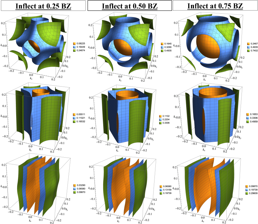
Figure 1: Contour plots of the paraboloid + inverted paraboloid band structure with inflection points at 0.25, 0.5, 0.75 way to the BZ boundaries. In the top row, $m_{x}=m_{y}=m_{z}=0.05$ (isotropic). In the middle row, $m_{x}=m_{y}=0.05$ and $m_{z}=5$. In the bottom row, $m_{x}=0.05$ and $m_{y}=m_{z}=5$. The energy scale is in Hartree.

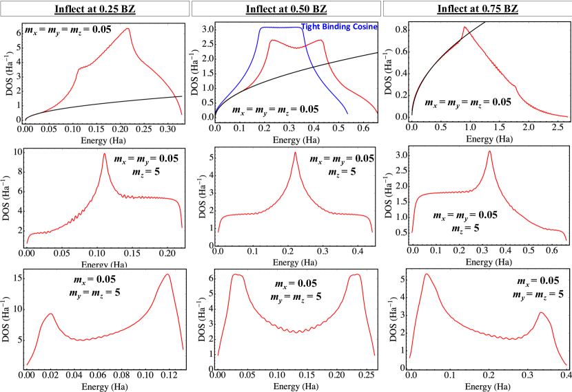
Figure 2: The density of states (red) of paraboloid + inverted paraboloid band structure with inflection points at 0.25, 0.5, 0.75 way to the BZ boundaries. In top row, $m_{x}=m_{y}=m_{z}=0.05$ (isotropy). The parabolic DOS of identical effective mass are plotted in black ($\sim\sqrt{(}E)$), which agree well with the initial upward-parabolic portion. For the isotropic band inflecting at 0.5 BZ, the similar tight-binding cosine DOS is plotted in blue for comparison. In middle row, $m_{x}=m_{y}=0.05$ and $m_{z}=5$ (unidirectional anisotropy), and the DOS onsets resemble the two-dimensional precipice.. In bottom row, $m_{x}=0.05$ and $m_{y}=m_{z}=5$ (bidirectional anisotropy), and the DOS onsets resemble the one-dimensional peak.

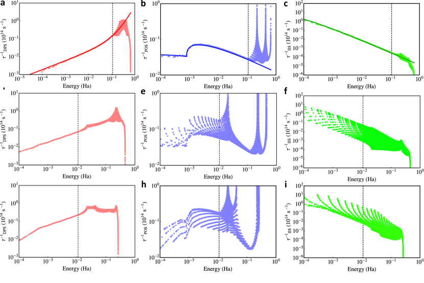
Figure 3: The k-dependent scattering rates plotted against energy for the paraboloid + inverted paraboloid band structure inflecting halfway to the zone-boundary. The vertical dashed lines demarcate the end of the purely upward-parabolic regime. a, d, g) Deformation-potential scattering (Eq. 11 in the main text), b, e, h) polar-optical scattering (Eq. 14 in the main text), and c, f, i) ionized-impurity scattering (Eq. 18 in the main text). a-c) Isotropic case, where $m_{x}=m_{y}=m_{z}=0.05$. Overlaid in solid lines are the energy-dependent scattering rates for a generic parabolic band of the same effective mass profile given by Eqs. 11, 13, and 15 in the main text. The agreements are essentially perfect in the upward-parabolic regime (before the dotted vertical lines), followed by deviations due to the downward inflection of our band. d-f) One-way-anisotropic case, where $m_{x}=m_{y}=0.05$ and $m_{z}=0.5$. g-i) Two-way-anisotropic case, where $m_{x}=0.05$ and $m_{y}=m_{z}=0.5$.

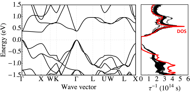
Figure 4: The band structure and electron-phonon scattering rates of Fe₂TiSi, with DOS overlaid in red. The scattering rates are calculated with the EPW software. The flat-and-dispersive conduction bands are dominated by DPS, which is essentially proportional to DOS. The valence bands are dominated by POS and does not scale as DOS as well ba2biau .

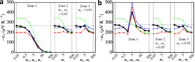
Figure 5: The Seebeck coefficient in the light direction ($x$) with the Fermi level fixed to the band minimum, as a function of changing effective masses in three directions. a) Single band evolves as depicted in Fig. 1a of the main text. b) Two bands exist where the second band evolves as depicted in Fig. 1b of the main text. Each zone indicates certain characteristic evolution: isotropic increase in $m$ from 0.05 to 500 in Zone 1, anisotropic increase in $m_{y}$ from 0.05 to 500 in Zone 2, anisotropic increase in both $m_{y}$ and $m_{z}$ in Zone 3 from 0.05 to 500. Four different scattering regimes are considered: the POS limit (blue), the IIS limit (green), the DPS limit (red), and the overall effect (black). The black dashed horizontal line marks the isotropic value.

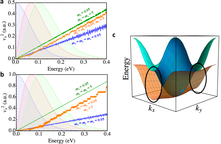
Figure 6: Schematics of factors that render band anisotropy’s effect on thermoelectric performance beneficial or harmful. a) Evolution of moving-averaged group velocities in the $x$ direction, $\langle v_{x}^{2}(E)\rangle$, for one-way anisotropy. b) Evolution of moving-averaged $\langle v_{x}^{2}(E)\rangle$ for two-way anisotropy. c) Dispersions of two paraboloid + inverted paraboloid bands, one isotropic (blue) and one very anisotropic (orange). Black circles mark the regions “low-energy voids,” where low-energy states exist for the latter but are absent for the former.

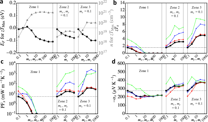
Figure 7: Same as Fig. 2 in the main text but with a larger $m_{x}=0.1$ and a higher $\kappa_{\text{lat}}=1$ W m^-1 K^-1.

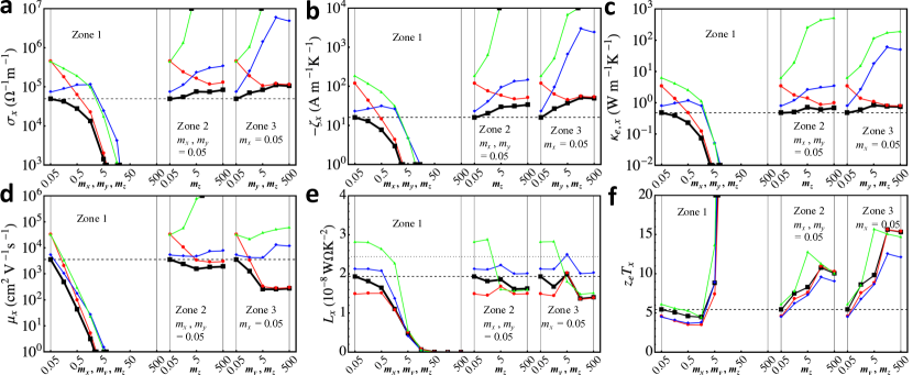
Figure 8: Supplement to Fig. 2 in the main text. Electronic transport properties in the light direction ($x$) for the single-band case, where horizontal dashed lines indicate the initial value at $m_{x}=m_{y}=m_{z}=0.15$. a) The charge (Ohmic) conductivities. b) The thermoelectric conductivities. c) The electronic thermal conductivities. d) Mobilities, which in the isotropic region decrease as $\mu_{\text{DPS}}\sim m^{-2.49}$, $\mu_{\text{POS}}\sim m^{-1.49}$, and $\mu_{\text{IIS}}\sim m^{-1.88}$. e) The Lorenz numbers, where the dotted line indicates the Wiedemann-Franz value ($L_{0}=2.44\times 10^{-8}$ W$\Omega$K^-2). f) The electronic-part $zT$.

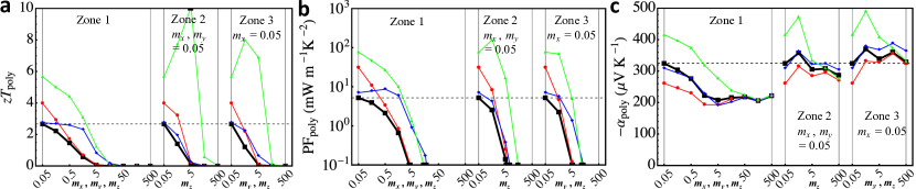
Figure 9: Polycrystalline thermoelectric properties of single band approximated by taking the harmonic mean of directional properties, supplemental electronic transport properties to Fig. 3 in the main text. a) $zT$, b) the PF, c) the Seebeck coefficient. The anisotropic zones 2 and 3 are marked by significantly worse performance compared to the single-light-direction performance provided in Fig. 2 in the main text. The isotropic zone 1 is identical to the single-direction trend.

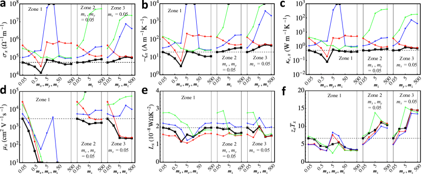
Figure 10: Supplement to Fig. 3 in the main text. Electronic transport properties in the light direction ($x$) for the two-band case, where horizontal dashed lines indicate the initial values for the single band case at $m_{x}=m_{y}=m_{z}=0.05$. a) The charge (Ohmic) conductivities. b) The thermoelectric conductivities. c) The electronic thermal conductivities. d) Mobilities, which in the isotropic region decrease as $\mu_{\text{DPS}}\sim m_{2}^{-2.46}$, $\mu_{\text{POS}}\sim m_{2}^{-1.37}$, and $\mu_{\text{IIS}}\sim m_{2}^{-1.81}$ where $m_{2}$ is the effective mass of the evolving second band. e) The Lorenz numbers, where the upper dotted horizontal line indicates the Wiedemann-Franz value ($L_{0}=2.44\times 10^{-8}$ W$\Omega$K^-2). f) The electronic-part $zT$.

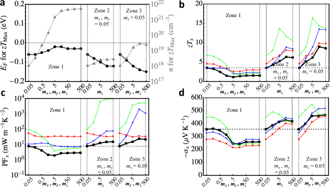
Figure 11: Same as Fig. 3 in the main text but with no interband scattering ($s_{\text{int}}=0$).

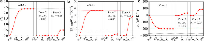
Figure 12: Thermoelectric properties in the light direction ($x$) with bipolar effect (zero band gap) as the valence band effective masses evolve and the conduction band is fixed at $m_{x}=m_{y}=m_{z}=0.05$, as in Fig. 1d in the main text. a) The power factor, b) the Seebeck coefficient, and c) $zT$. Each zone indicates certain characteristic evolution of the valence band: isotropic increase in $m$ from 0.05 to 500 in Zone 1, anisotropic increase in $m_{y}$ from 0.05 to 500 in Zone 2, anisotropic increase in both $m_{y}$ and $m_{z}$ in Zone 3 from 0.05 to 500. Only DPS is considered due to the metallic assumption (very high carrier concentrations). The red horizontal dashed lines indicate the single-conduction-band (i.e. insulating state) values under DPS scattering only, and the black horizontal dashed lines indicate those under the overall effect of POP and IIS as well as DPS.

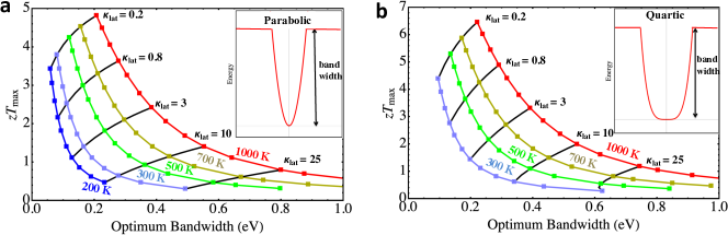
Figure 13: $T$-and-$\kappa_{\text{lat}}$-dependent optimum bandwidth and $zT$ under DPS and fixed $E_{\text{F}}=0$ for a) an isotropic 3D parabolic band of $m_{\text{GaAs}}=0.067$, and b) an isotropic 3D quartic with the same energy as the parabolic band at the inflection point. The Fermi level here is fixed at the respective CBM for comparison purposes. $\kappa_{\text{lat}}$ is given in W m^-1K^-1.

II Supplementary Discussion

A review of the single parabolic band model and the Pisarenko formulas for the Seebeck coefficient is in order owing to their generality, wide reference, and limitations our study improves upon. The Seebeck coefficient is, in the degenerate or metallic limit,

$$\alpha=\frac{\pi^{2}k_{\text{B}}^{2}T}{3E_{\text{F}}}=\frac{2k_{\text{B}}^{2}}{3}mT\left(\frac{\pi}{3n}\right)^{\frac{2}{3}},$$ (1)

and in a non-degenerate case,

$$\alpha =k_{\text{B}}\left(\frac{5}{2}+s-\frac{E_{\text{F}}}{k_{\text{B}}T}\right)$$ (2)

$$=k_{\text{B}}\left(\frac{5}{2}+s+\text{log}\left(n^{-1}\left(\frac{mk_{\text{B}}T}{2\pi}\right)^{\frac{3}{2}}\right)\right),$$

where $n$ is carrier concentration, $m$ is the band effective mass, $k_{\text{B}}$ is the Boltzmann constant, and $s$ is the power of energy to which carrier lifetimes are proportional ($\tau\propto E^{s}$). Contrary to a widely held notion, a heavier band (high $m$) does not by default generate higher Seebeck coefficient under this model since $\alpha$ can be written as a function of either $E_{\text{F}}$ or $m$-and-$n$, where the trivial exchange of variables is allowed by their interrelations:

$$E_{\text{F}}=\frac{\pi^{2}}{2m}\left(\frac{3n}{\pi}\right)^{\frac{2}{3}}$$ (3)

in the degenerate case, and

$$\frac{E_{\text{F}}}{k_{\text{B}}T}=\text{log}\left(n^{-1}\left(\frac{mk_{\text{B}}T}{2\pi}\right)^{\frac{3}{2}}\right)$$ (4)

in the non-degenerate case. Equations 1–2 stipulate that, if $E_{\text{F}}$ is fixed, then $\alpha$ is constant whatever the $m$ value because $n$ would change accordingly. A light band with a small $m$ would produce the same Seebeck coefficient as a heavier band with a larger $m$ provided that $E_{\text{F}}$ is kept fixed.

The lead-up to Eqs. 1–2 bears one hidden but critical assumption: that there is always enough (infinite) dispersion in all directions to cover the entire energy range relevant to thermoelectric phenomena. However, it breaks down when a band becomes critically heavy that it reaches the BZ boundary before gaining enough energy to cover the entire relevant energy range for transport. Also, because a true solid-state band must at some point change in curvature from positive to negative and cross the BZ boundary orthogonally, there comes a point where assuming constant positive curvature introduces additional unrealistic effects. As will be seen, these effects lead to some conclusions that deviate from what would otherwise be drawn from Eqs. 1–2. Other assumptions in typical parabolic band models include absence of opposing bands (bipolar effect) and a monotonically behaved, or at least slow-varying, $\Sigma(E)$ such that the Sommerfeld expansion is valid, a requirement for arriving at Eqs. 1–2.

To demonstrate the importance of our method, we calculate our model-predicted Seebeck coefficient $\alpha$ with a fixed $E_{\text{F}}$ at the band minimum. This exercise helps clarify the difference in behavior of our model versus previous models including SPB, and also clearly illustrates the concept of improving $\zeta$ relative to $\sigma$ via band structure alone. The results are plotted in Supplementary Fig. 5.

The fixed-$E_{\text{F}}$ results for single band evolution as depicted in Fig. 1a of the main text are given in Supplementary Fig. 5a. The main takeaway from Zone 1 is the problem of insufficient dispersion for critically heavy bands. We observe that $\alpha$ starts on a plateau that corresponds to the classic SPB model behavior. When the band becomes critically heavy, however, $\alpha$ starts to decrease below the SPB value. The origin of this deviation is that the band becomes heavy enough to terminate at the BZ boundary before gaining enough energy to fully trigger $\zeta$, and misses out on some high-energy states that would otherwise contribute relatively more to $\zeta$ than $\sigma$. For example, at 500 K, carriers of up to 0.18 eV and 0.25 eV above the Fermi level make 97% of the total contribution to respectively $\sigma$ and $\zeta$. However in our model, if $m=5$, the band encounters the BZ boundary at a value of 0.18 eV, which is enough to almost entirely trigger $\sigma$ but miss important contributions to $\zeta$. Any further increase in $m$ translates to increasingly greater relative loss for $\zeta$ than $\sigma$, continuously degrading the Seebeck coefficient. Typical SPB models overlook this problem of insufficient dispersion owing to the finite-sized BZ, breaking down for heavy enough dispersions. Of note, $\alpha$ goes to 0 as the band completely flattens out, which is explained in the later discussions on optimum bandwidth.

The main lesson from Zones 2 and 3 in Supplementary Fig. 5a, where the band evolves anisotropically, is the role of group velocity. Under DPS and to a lesser extent under POS, we observe that moderate anisotropy gives the highest $\alpha$, represented by the $\alpha$ peak in the middle of the two zones ($m_{y},m_{z}=5$). Because $\Sigma(E)\propto v^{2}(E)$ under DPS, thermoelectric behaviors are determined entirely by the average group velocities, $\langle v_{x}^{2}(E)\rangle$. For an isotropic parabolic band, $\langle v^{2}(E)\rangle=\frac{2mE}{3}$; thus, the contribution to $\Sigma(E)$ scales linearly with $E$. For a moderately anisotropic band, $\langle v_{x}^{2}(E)\rangle$ develops a kink. That is, it abruptly steepens in slope (see supplementary Figs. 6a–b). Specifically, for unidirectional anisotropy (heavy only in $z$), $\langle v_{x}^{2}(E)\rangle\propto mE$ post-kink which is the 2D parabolic velocity scaling. For bidirectional anisotropy (heavy in $y$ and $z$), $\langle v_{x}^{2}(E)\rangle\propto 2mE$ post-kink which is the even steeper 1D parabolic velocity scaling. Relative to the scaling of an isotropic band, the kinked $\langle v_{x}^{2}(E)\rangle$ profiles weight $\zeta$ more than $\sigma$ because the velocities increase more steeply at higher energies that at lower energies. This allows $\alpha$ to peak at some moderate anisotropy, and the peak is higher for bidirectional anisotropy. For extremely anisotropic bands mimicking low-dimensional bands, which are also popularly known as “flat-and-dispersive” bands lowdimensional3d ; quantumwell , $\langle v_{x}^{2}(E)\rangle$ reverts to linear scaling but with the steeper, post-kink slopes.

Another subtlety regarding extremely anisotropic bands is that they exhaust “low-energy voids”. That is to say, wherever carriers line up along the heavy direction(s), their dispersion in the light direction starts from essentially the band minimum energy. This poses a stark contrast to a less anisotropic band or an isotropic band, for which some dispersion towards the light direction may start from higher energies leaving behind a void of states at lowest energies (see Supplementary Fig. 6c). Because low-energy states contribute relatively more to $\sigma$ than to $\zeta$, their absence is a clear benefit to thermoelectrics. Extremely anisotropic bands exhaust these voids, and therefore, the overall $\alpha$ is somewhat lower than in the isotropic case. POS retains some of the same $\alpha$ signatures of DPS, while under IIS $\alpha$ only decreases with anisotropy.

Next, we examine the case of two bands whose results are in Supplementary Fig. 5b. Here, we fix the first band in shape and evolve the second band mass according to Fig. 1b in the main text. The results are largely similar to the single-band results but for a prominent peak in $\alpha$ in the middle of Zone 1 (under DPS and POS) where the second band flattens out isotropically. This peak represents the second band acting as a resonance level resonancelevelreview that performs energy-filtering due to interband scattering. Although the isotropically heavy band has negligible direct contribution to transport, it can act as a localized scattering partner for the dispersive principal band where their energies overlap, or “resonate,” thereby preferentially scattering low-energy carriers. This increases $\zeta$ relative to $\sigma$ because the low-energy states that had previously contributed much more to $\sigma$ than $\zeta$ are now selectively scattered by the narrowed second band. As a result, $\alpha$ is able to well exceed its single-dispersive-band value. As the second band completely flattens out, however, its width becomes too narrow to filter enough states and hence $\alpha$ is reduced again. We observe that IIS is not a good agent of energy-filtering.

In summary, whereas $\alpha$ is constant for any band under the SPB model as long as $E_{\text{F}}$ is fixed, our revised model correctly reflects its fluctuating response to changes in a band structure, especially as it approaches extreme shapes.

The optimum $E_{\text{F}}$, plotted in Fig. 2a of the main text, is entirely below the band minimum (zero). This can be understood by noting that generally $\kappa_{e}>>\kappa_{\text{lat}}$ in our model, which in turn leads to $zT\approx\frac{\alpha^{2}}{L}$ where $L$ is the Lorenz number. In the absence of bipolar effect, because $\alpha$ is higher at lower $E_{\text{F}}$ whereas $L$ is relatively constant with respect to $E_{\text{F}}$, $zT$ peaks at low $E_{\text{F}}$ (non-degenerate doping) near where $\alpha$ peaks.

The optimum $E_{\text{F}}$ fluctuates with band evolution. In Zone 1, initially, optimal $E_{\text{F}}$ increases as the band turns heavier. This is because, as the band turns heavier, $\kappa_{e}$ becomes comparable to and then lower than $\kappa_{\text{lat}}$. When $\kappa_{e}<\kappa_{\text{lat}}$, higher PF is required to drive high $zT$. Because the PF is maximized with $E_{\text{F}}$ near the band minimum, optimal $E_{\text{F}}$ increases to meet it. When the band becomes critically heavy and narrow in Zone 1, optimal $E_{\text{F}}$ reverses course and moves away from the band minimum. This is because $E_{\text{F}}$ must again be placed at a distance from the band minimum in order to generate finite $\alpha$ for reasons explained in the later discussions regarding optimum bandwidth.

In Zones 2 and 3, as the band turns anisotropic, $\zeta$ and $\kappa_{e}$ both increase relative to $\sigma$ due to steepening group velocity profile. Because $\kappa_{e}$ increases relative to $\kappa_{\text{lat}}$, which is fixed in our model, $zT$ is increasingly less needy of high PF, and peaks at increasingly lower $E_{\text{F}}$ near where $\alpha$ is maximized.

In Fig. 3a in the main text, describing the multi-band context, the optimal $E_{\text{F}}$ behaves largely similar as it does in Fig. 2a except for the huge spike in the center of Zone 1. A spike in optimal $E_{\text{F}}$, through the band, corresponds to the case where the resonance effect is the most pronounced. Because low-energy states are heavily scattered due to the second band performing energy-filtering, $\zeta$ does not suffer bipolar reduction even if these low-energy states are placed on the opposite side of the Fermi level. Neither does $\sigma$ significantly increase. In turn, $zeta$ benefits from larger $\Sigma(E)$ of the deeper conduction states. When the second band becomes too narrow to act as a resonance level, the optimal $E_{\text{F}}$ again falls below the band minimum as in the single-band case of Fig. 2a.

For a simple study of bipolar effect, we fix the band gap to 0 such that the two bands are tangent to one another at $k=0$ and $E=0$. Note that the band gap is an adjustable parameter in our model. We then fix the dispersion of the conduction band and modulate the valence band effective masses (see Fig. 1c in the main text). Two tangent bands are admittedly not how realistic metallic band structures usually are, but nonetheless, this set-up does probe the essence of how bipolar effect could be resisted for metals and tiny-gap semiconductors. We consider only DPS since the very high $n$ in metals would virtually completely screen Coulombic mechanisms that are POS and IIS.

The message of Supplementary Fig. 12 is straightforward: bipolar negation of the Seebeck coefficient is suppressed if one band is light and the opposing band is heavy, or more specifically if there is an asymmetry in $\Sigma(E)$ about the Fermi level. The greater the contrast, the better, though the benefit effectively saturates past a point. From the $n$-type point of view, a completely flat valence band would not carry any hole current but only function as a potential resonance level for low-energy electrons (would require inelastic processes). The desired effect in this picture is essentially a hybrid of the light-band-over-heavy-band rule and energy-filtering: keep holes heavy and filter them further out with as much resonance scattering as possible, while keeping electrons mobile and scattering-free except at very low energies. It is worth recognizing that, in the limit of completely flat valence band, one essentially has a degenerate-semiconducting state with a resonance level and a “gap” below. This indicates that, within the conventional setting herein assumed, the ideal limit for a metallic thermoelectric is precisely the semiconducting limit with only DPS being present. The identity of the rightmost $zT$ values (under DPS) in each zone in Figs. 3a (main text) and 12a proves the point.

Lastly for metals and tiny-gap semiconductors, $\kappa_{e}$ is frequently far higher than $\kappa_{\text{lat}}$, where small Lorenz number ($L=\frac{\kappa_{e}}{\sigma T}$) becomes critical. Even for typical semiconductors, once $\kappa_{\text{lat}}$ is reduced and the PF is improved, realizing small $L$ would be the final piece of the puzzle. Mirroring the way in which bipolar transport is fought, it is theoretically rather clear what must be done to achieve small $L$: filter out very high-energy states because they contribute relatively more to the thermal current than the thermoelectric or Ohmic currents. They could, in theory, be either 1) filtered with additional states that locally accommodate heavy scattering at high energies, or 2) better yet by simple absence of high-energy states.

Investigation of optimal electronic structures for thermoelectrics can be traced back to the seminal work by Mahan and Sofo bestthermoelectric . They took a purely mathematical approach to formulate $zT$ in terms of the energy integrals presented in the main text, and derived the ideal spectral conductivity for maximization of $zT$. They determined that a Dirac delta function near the Fermi level, say at $E_{\dagger}\approx E_{\text{F}}$, is the ideal functional form:

$$\Sigma(E)=D(E)v^{2}(E)\tau(E)=\Sigma_{0}\delta_{E,E^{\dagger}},$$ (5)

where $\Sigma_{0}$ is some pre-factor. $D(E)$ and $v^{2}(E)$ are directly determined by the electronic structure, while $\tau(E)$ is only indirectly related to it and heavily depends on electron scattering mechanisms. However, their approach was purely mathematical in nature with an implicit assumption that $\kappa_{\text{lat}}=0$. Supplementary Eq. 5 must be interpreted with caution when applied to reality.

For Supplementary Eq. 5 to be satisfied, mathematically, at least one of $D(E)$, $v^{2}(E)$, or $\tau(E)$ must be $\delta_{E,E^{\dagger}}$. Physically, however, the terms cannot be independently reduced to a delta function. Firstly, $v^{2}(E)$ cannot be $\delta_{E,E^{\dagger}}$ while $D(E)$ is not, because $v^{2}(E)$ is categorically zero without some band dispersion around $E_{\text{F}}$, while no band dispersion can arise at all if $D(E)$ has no width. Secondly, provided there is some dispersion, $\tau(E)$ cannot be a delta function unless electrons are perfectly scattered everywhere but at single $E_{\text{F}}$, which is next to impossible. Then the only plausible way in which $\tau(E)$ can be a delta function is if $D(E)$ is also. These considerations indicate that the only way for Supplementary Eq. 5 to hold is for $D(E)=N_{v}\delta_{E,E^{\dagger}}$, reflecting one or more ($N_{v}$) perfectly localized states, or perfectly flat bands. The factor $N_{v}$ arises from the fact that eDOS of each band must integrate to 1 (or 2 if spin-degenerate) to conserve the number of electrons:

$$N_{v}=\sum_{1}^{N_{v}}\int_{-\infty}^{\infty}\delta_{E,E^{\dagger}}dE.$$ (6)

This in turn forces $\tau(E)=\tau_{0}\delta_{E,E^{\dagger}}$ for some finite $\tau_{0}$ limited by elastic scattering, but more importantly it forces $v_{0}\rightarrow 0$ and therefore by default $\Sigma(E)\rightarrow 0$.

The implications of $\Sigma(E)\rightarrow 0$ are as follows. First, the conductivity is immediately 0, as has also been pointed out by a previous study optimalbandwidth ,

$$\sigma=\int_{-\infty}^{\infty}\Sigma(E)\left(-\frac{\partial f}{\partial E}\right)dE=0.$$ (7)

Second, the Seebeck coefficient is expressible as the following limit as $\Sigma(E)\rightarrow 0$ point-by-point:

$$\alpha=\lim_{\Sigma(E)\rightarrow 0}\frac{\frac{1}{T}\int_{-\infty}^{\infty}\Sigma(E)(E_{\text{F}}-E)\left(-\frac{\partial f}{\partial E}\right)dE}{\int_{-\infty}^{\infty}\Sigma(E)\left(-\frac{\partial f}{\partial E}\right)dE}.$$ (8)

Generally speaking, this is a non-trivial limit to evaluate because $\Sigma(E)$ is a function, not a scalar. However, with the knowledge that $\Sigma(E)$ is widthless (due to $D(E)$), and so it would approach zero at a single point, we can reformulate the limit as

$$\lim_{\Sigma(E)\rightarrow 0}\Sigma(E)=\lim_{n\rightarrow\infty}\frac{1}{n}\Sigma_{0}\delta_{E,E^{\dagger}},$$ (9)

where $n\geq 1$ is an integer, and evaluate Supplementary Eq. 8 as

$$\alpha =\lim_{n\rightarrow\infty}\frac{\frac{1}{n}\frac{1}{T}\int_{-\infty}^{\infty}\Sigma_{0}\delta_{E,E^{\dagger}}(E_{\text{F}}-E)\left(-\frac{\partial f}{\partial E}\right)dE}{\frac{1}{n}\int_{-\infty}^{\infty}\Sigma_{0}\delta_{E,E^{\dagger}}\left(-\frac{\partial f}{\partial E}\right)dE}$$ (10)

$$=\frac{1}{T}(E_{\text{F}}-E^{\dagger}),$$

and this behavior is graphically verified in Fig. 2a and Fig. 3c in the main text. In Fig. 2a, where $E^{\dagger}$ tends to $E_{\text{F}}$ at the band minimum as the band narrows, $\alpha$ tends to 0. In Fig. 3c, where $E^{\text{F}}$ is away from the band minimum that $E^{\dagger}$ tends to, $\alpha$ tends to some finite value corresponding to $(E_{\text{F}}-E^{\dagger})$.

Third, by the same token as above, the Lorenz number can be shown to tend to 0 for a widthless band:

$$L =\lim_{n\rightarrow\infty}\frac{\frac{1}{n}\left[\frac{1}{T}\int_{-\infty}^{\infty}\Sigma_{0}\delta_{E,E^{\dagger}}(E_{\text{F}}-E)^{2}\left(-\frac{\partial f}{\partial E}\right)dE-T\alpha^{2}\int_{-\infty}^{\infty}\Sigma_{0}\delta_{E,E^{\dagger}}\left(-\frac{\partial f}{\partial E}\right)dE\right]}{\frac{1}{n}\int_{-\infty}^{\infty}\Sigma_{0}\delta_{E,E^{\dagger}}\left(-\frac{\partial f}{\partial E}\right)dE}$$ (11)

$$=\frac{1}{T}(E_{\text{F}}-E^{\dagger})^{2}-\frac{1}{T}(E_{\text{F}}-E^{\dagger})^{2}=0,$$

and this behavior is graphically suggested in Supplementary Fig. 8e. By Eqs. 10 and 11, given some $E^{\dagger}$, a perfectly localized band of widthless $D(E)$ would lead to divergence in “electronic-part $zT$,” or $zT$ without $\kappa_{\text{lat}}$:

$$z_{e}T=\frac{\alpha^{2}\sigma}{\kappa_{e}}T=\frac{\alpha^{2}}{L}=\infty.$$ (12)

This behavior, consistent with the conclusions of the Mahan-Sofo theory, is graphically suggested in Supplementary Fig. 8f. However, because of finite Seebeck and vanishing conductivity, the PF would vanish, and compounded by $\kappa_{\text{lat}}>0$ in real materials, $zT$ would vanish to 0 alike. Ergo, even if a set of perfectly localized states could exist in real materials, it is not the physically ideal structure for $zT$ or the PF in real materials. The fundamental barrier is, again, that the components of $\Sigma(E)$ cannot be independently widthless. The value of $z_{e}T$ as a metric for thermoelectric performance improves only as $v(E)$ becomes finite and large and as $\kappa_{\text{lat}}$ is kept minimal.

In supplement to the optimum bandwidth of a parabolic band, we also consider an isotropic quartic band, $E=c(k_{x}^{2}+k_{y}^{2}+k_{z}^{2})^{2}$. The quartic dispersion coefficient $c$ is selected such that it gives the quartic band the same energy as the parabolic band at the inflection point. Supplementary Fig. 13 shows the results. Between parabolic and quartic dispersions, we see that the latter performs better by about 20%. Since $\tau\propto D^{-1}(E)$ under DPS, it is again the average group velocities distribution that is responsible for the better quartic performance in the transport direction: $\langle v_{x}^{2}(E)\rangle=\frac{16\sqrt{c}}{3}E^{1.5}$. This obviously grows faster with $E$ than that for the parabolic $\langle v_{x}^{2}(E)\rangle=\frac{2}{3m}E$, thereby weighting $\zeta$ relatively more than $\sigma$.

III Supplementary Methods

The deformation-potential scattering was initially developed for long-wavelength acoustic phonon scattering defpotbardeenshockley . Even with the Kahn-Allen correction defpotkahnallen that we introduce, the overall DPS rate follows the DOS for the most part. However, as mentioned in the main text, the $\tau^{-1}_{\text{DPS}}\propto D(E)$ model works very well in practice for very anisotropic bands in the presence of zone-boundary phonon scattering as well as interband scattering. This was verified by accurate first-principles calculation of electron-phonon scattering using the EPW software epw1 ; epw3 for materials such as Fe₂TiSi ba2biau and Li₂TlBi analoguepbte .

Fe₂TiSi conduction bands are flat-and-dispersive and dominated by DPS ba2biau . The scattering rate for the conduction bands closely follow DOS, which validates the $\tau^{-1}_{\text{DPS}}\propto D(E)$ model. The valence bands are affected significantly by POS, and their scattering rates deviate from DOS. See Supplementary Fig. 4. Li₂TlBi valence bands are flat-and-dispersive and dominated by DPS analoguepbte . The scattering rate for the valence bands closely follow DOS, which again validates the $\tau^{-1}_{\text{DPS}}\propto D(E)$ model..

Therefore, we expect the extension of Eqs. 10 and 11 in the main text to work well for our model band structures.

For a parabolic band, there exists an analytic formula for energy-dependent lifetime due to inelastic POS lundstrom ; nolassharpgoldsmid ,

$$\tau_{\text{POS}}(E)=\frac{E^{\frac{1}{2}}}{\sqrt{2}\omega_{o}m^{\frac{1}{2}}}\left(\frac{1}{\epsilon_{\infty}}-\frac{1}{\epsilon}\right)^{-1}\left[(b(\omega_{o})+1)\cdot\text{sinh}^{-1}\left(\sqrt{\frac{E}{\omega_{o}}-1}\right)+b(\omega_{o})\cdot\text{sinh}^{-1}\left(\sqrt{\frac{E}{\omega_{o}}}\right)\right]^{-1}.$$ (13)

The first (second) term in the square brackets represents emission (absorption). However, derivation of Supplementary Eq. 13 uses an energy-momentum phase-space integral simplified with a parabolic dispersion relation, rendering its direct application to non-parabolic bands unjustified. The hyperbolic arcsin terms account for the availability of DOS ($\sim\sqrt{E}$ for a parabolic band) for carriers to be scattered into (final states). Our correction in the main text makes partial corrections by utilizing custom-calculated DOS and k-dependent forms of Supplementary Eq. 13.

The established energy-dependent formalism for IIS of a parabolic band is the Brooks-Herring formula brooks ; ionizedimpurity ,

$$\tau_{\text{IIS}}(E)=\frac{\sqrt{2}\epsilon^{2}m^{\frac{1}{2}}E^{\frac{3}{2}}}{\pi N_{i}Z^{2}}\left(\text{log}(1+\gamma(E))-\frac{\gamma(E)}{1+\gamma(E)}\right)^{-1},$$ (14)

where $\gamma$ is a screening term defined as,

$$\gamma(E)=\frac{8mE\epsilon k_{\text{B}}T}{n}\left(\frac{F_{\frac{1}{2}}(E_{\text{F}})}{F_{-\frac{1}{2}}(E_{\text{F}})}\right).$$ (15)

and $F_{z}(E_{\text{F}})$ is the Fermi-Dirac integral

$$F_{z}(E_{\text{F}})=\frac{1}{\Gamma(z+1)}\int_{0}^{\infty}\frac{y^{z}}{1+\text{exp}(y-\frac{E_{\text{F}}}{k_{\text{B}}T})}dy.$$ (16)

Its derivation involves k-space integration over spherical isoenergy surfaces of a parabolic band, rendering it also non-trivial to extend to non-parabolic bands. Our correction in the main text makes partial corrections by utilizing custom-calculated DOS and k-dependent forms of Supplementary Eqs. 14–15.

IV Supplementary References

References

- (1) Park, J., Xia, Y., Ozoliņš, V. High Thermoelectric Power Factor and Efficiency from a Highly Dispersive Band in Ba2BiAu. Phys. Rev. Appl. 11, 1 (2019).
- (2) Parker, D., Chen, X., Singh, D. J. High Three-Dimensional Thermoelectric Performance from Low-Dimensional Bands. Phys. Rev. Lett. 119, 14 (2013).
- (3) Hicks, L. D., Dresselhaus, M. Effect of quantum-well structures on the thermoelectric Figure of merit. Phys. Rev. B 47, 19 (1993).
- (4) Heremans, J. P., Wiendlochaac, B., Chamoire, A. M. Resonant levels in bulk thermoelectric semiconductors. Energy Environ. Sci. 5:5510–5530 (2012).
- (5) Mahan, G. D., Sofo, J. The Best Thermoelectric. Proc. Natl. Acad. Sci. 93:7436–7439 (1996).
- (6) Zhou, J., Yang, R., Chen, G., , Dresselhaus, M. S. Optimal Bandwidth for High Efficiency Thermoelectrics. Phys. Rev. Lett. 108:226601 (2011).
- (7) Bardeen, J., Shockley, W. Deformation Potentials and Mobilities in Non-Polar Crystals. Phys. Rev. 80, 1 (1950).
- (8) Khan, F. S., Allen, P. B. Deformation potentials and electron-phonon scattering: Two new theorems. Phys. Rev. B 29, 6 (1984).
- (9) Giustino, F., Cohen, M. L., Louie, S. G. Electron-phonon interaction using Wannier functions. Phys. Rev. B 76, 16 (2007).
- (10) Ponce, S., Margine, E. R., Verdi, C., Giustino, F. EPW: Electron–phonon coupling, transport and superconducting properties using maximally localized Wannier functions. Comput. Phys. Commun. 55:116–133 (2016).
- (11) He, J., Xia, Y., Naghavi, S. S., Ozoliņš, V., Wolverton, C. Designing chemical analogs to PbTe with intrinsic high band degeneracy and low lattice thermal conductivity. Nat. Commun. 10, 719 (2019).
- (12) Lundstrom, M. Fundamentals of Carrier Transport. (Cambridge University Press 2000).
- (13) Nolas, G. S., Sharp, J., Goldsmid, H. J. Thermoelectrics. (Springer 2001).
- (14) Brooks, H. Theory of the Electrical Properties of Germanium and Silicon. Adv. Elec. Elec. Phys. 7:85–182 (1955).
- (15) Chattopadhyay, D., Queisser, H. J. Electron Scattering by Ionized Impurities in Semiconductors. Rev. Mod. Phys. 53, 4 (1981).