Approximate information state for approximate planning and reinforcement learning in partially observed systems

Abstract

We propose a theoretical framework for approximate planning and learning in partially observed systems. Our framework is based on the fundamental notion of information state. We provide two equivalent definitions of information state—i) a function of history which is sufficient to compute the expected reward and predict its next value; ii) equivalently, a function of the history which can be recursively updated and is sufficient to compute the expected reward and predict the next observation. An information state always leads to a dynamic programming decomposition. Our key result is to show that if a function of the history (called approximate information state (AIS)) approximately satisfies the properties of the information state, then there is a corresponding approximate dynamic program. We show that the policy computed using this is approximately optimal with bounded loss of optimality. We show that several approximations in state, observation and action spaces in literature can be viewed as instances of AIS. In some of these cases, we obtain tighter bounds. A salient feature of AIS is that it can be learnt from data. We present AIS based multi-time scale policy gradient algorithms. and detailed numerical experiments with low, moderate and high dimensional environments.

Keywords: Partially observed reinforcement learning, partially observable Markov decision processes, approximate dynamic programming, information state, approximate information state.

1 Introduction

Reinforcement learning (RL) provides a conceptual framework for designing agents which learn to act optimally in an unknown environment. RL has been successfully used in various applications ranging from robotics, industrial automation, finance, healthcare, and natural language processing. The success of RL is based on a solid foundation of combining the theory of exact and approximate Markov decision processes (MDPs) with iterative algorithms that are guaranteed to learn an exact or approximate action-value function and/or an approximately optimal policy (Sutton and Barto, 2018; Bertsekas and Tsitsiklis, 1996). However, for the most part, the research on RL theory is focused primarily on systems with full state observations.

In various applications including robotics, finance, and healthcare, the agent only gets a partial observation of the state of the environment. Such partially observed systems are mathematically modeled as partially observable Markov decision processes (POMDPs) and there is a fairly good understanding of how to identify optimal or approximately optimal policies for POMDPs when the system model is known to the agent.

Since the initial work on POMDPs (Aström, 1965), it is known that POMDPs can be modeled as fully observed MDPs by considering the belief state (i.e., the posterior belief of the unobserved state given all the observations made by the agent) as an information state. Therefore, the theory and algorithms for exact and approximate planning for MDPs are also applicable to POMDPs. One computational challenge is that the belief state is continuous valued. However, the value function based on the belief state has a nice property—it is piecewise linear and a convex function of the belief state—which can be exploited to develop efficient algorithms to identify the optimal policy. Building on the one-pass algorithm of (Smallwood and Sondik, 1973), various such algorithms have been proposed in the literature including the linear support algorithm (Cheng, 1988), the witness algorithm (Cassandra et al., 1994), incremental pruning (Zhang and Liu, 1996; Cassandra et al., 1997), the duality based approach (Zhang, 2009), and others. Since POMDPs are PSPACE-complete (Papadimitriou and Tsitsiklis, 1999), the worst case complexity of such algorithms is exponential in the size of the unobserved state space. To overcome the worst case complexity of finding an optimal policy, various point-based methods have been proposed in the literature which obtain an approximate solution by sampling from the belief space (Pineau et al., 2003; Smith and Simmons, 2004; Spaan and Vlassis, 2005; Shani et al., 2007; Kurniawati et al., 2008; Poupart et al., 2011); see Shani et al. (2013) for an overview and comparison.

However, the exact and approximate planning results are of limited value for partially observed reinforcement learning (PORL) because they are based on the belief state, constructing which requires the knowledge of the system model. So, when an agent is operating in an unknown environment, it cannot construct a belief state based on its observations. An attempt to circumvent this difficulty was to use memoryless policies (i.e., choose the action based only on the current observation) (Littman, 1994; Loch and Singh, 1998; Jaakkola et al., 1995; Williams and Singh, 1999; Li et al., 2011; Azizzadenesheli et al., 2016). A related idea is to choose the action based on $k$ recent observations (Littman, 1994; Loch and Singh, 1998) or choose the action based on a memory which is updated using a finite state machine (Whitehead and Lin, 1995; McCallum, 1993; Hansen, 1997; Meuleau et al., 1999; Amato et al., 2010). Such finite memory policies are also amenable to policy search methods (Hansen, 1998; Baxter and Bartlett, 2001; Poupart and Boutilier, 2004). However, there are no approximation guarantees available for such methods.

Another approach taken in the literature is to use a Bayesian RL framework (Ross et al., 2008; Poupart and Vlassis, 2008; Ross et al., 2011; Katt et al., 2019) where a posterior distribution over the models of the environment is maintained; at each step, a model is sampled from the posterior and the corresponding optimal policy is executed. Appproximation error bounds in using such methods are derived in Ross et al. (2011).

A completely different class of model-based RL algorithms are methods using predictive state representations (PSRs) (Littman et al., 2002; Singh et al., 2003). PSRs are constructed only based on observational data so they can easily be adapted to the RL setup. There have been a number of papers which use PSRs to propose model based RL algorithms (James et al., 2004; Rosencrantz et al., 2004; Boots et al., 2011; Hamilton et al., 2014; Kulesza et al., 2015b, a; Jiang et al., 2016).

Inspired by the recent successes of deep reinforcement learning, there are many recent results which suggest using RNNs (Recurrent Neural Networks (Rumelhart et al., 1986)) or LSTMs (Long Short-Term Memories (Hochreiter and Schmidhuber, 1997)) for modeling the action-value function and/or the policy function (Bakker, 2002; Wierstra et al., 2007, 2010; Hausknecht and Stone, 2015; Heess et al., 2015; Zhu et al., 2017; Ha and Schmidhuber, 2018; Baisero and Amato, 2018; Igl et al., 2018; Zhang et al., 2019). It is shown that these approaches perform well on empirical benchmarks, but there are no approximation guarantees available for such methods.

Our main contribution is to present a rigorous approach for PORL which is based on a principled theory of approximate planning for POMDPs that we develop. In particular:

1. In Sec. 2, we formalize the notion of information state for partially observed systems and provide equivalent methods of identifying information states.

2. In Secs. 3 and 4, we present the notion of an approximate information state (AIS) as a compression of history which approximately satisfies the properties of an information state. The two equivalent formulations of information state lead to two equivalent formulations of AIS. We present bounds on the loss in performance (compared to the optimal history dependent policy) when planning using an AIS. We generalize these results to cover approximation in action spaces as well. We show that various existing approximation results for MDPs and POMDPs in the literature may be viewed as special cases of AIS (and in some cases, our bounds are tighter than those in the literature).

3. In Sec. 5, we present a theory for approximate planning for decentralized (i.e., multi-agent) partially observed systems using a common-information based AIS.

4. In Secs. 6 and 7, we then present policy gradient based online RL algorithms for PORL which learn an AIS representation using multi-timescale stochastic gradient descent. We provide detailed numerical experiments on several classes of partially observed environments ranging from classical low-dimensional toy environments, to moderate-dimensional environments, and high-dimensional grid-world environments.

2 Preliminaries: Information state and dynamic programming decomposition for partially observed systems

2.1 General model for a partially observed system

Traditionally, partially observed systems are modeled as partially observable Markov decision processes (POMDPs) (Aström, 1965; Smallwood and Sondik, 1973), where there is a controlled state and an agent which makes noise corrupted observations of the state. However, for the purpose of understanding approximation for partially observed systems, it is conceptually cleaner to start with an input-output model of the system as described below.

Figure 1: A stochastic input-output system

Figure 2: The timing diagram of the input-output system.

We view a partially observed system as a black-box input-output system shown in Fig. 2. At each time $t$, the system has two inputs and generates two outputs. The inputs to the system are a control input (also called an action) $A_{t}\in\mathsf{A}$ and a disturbance $W_{t}\in\mathsf{W}$. The outputs of the system are an observation $Y_{t}\in\mathsf{Y}$ and a reward $R_{t}\in\mathbb{R}$. For the ease of exposition, we assume that $\mathsf{A}$, $\mathsf{W}$, and $\mathsf{Y}$ are finite sets. The analysis extends to general spaces under appropriate technical conditions. The order in which the input and output variables are generated is shown in Fig. 2.

As stated before, we do not impose a state space model on the system. Therefore, all we can say is that the outputs $(Y_{t},R_{t})$ at time $t$ are some function of all the inputs $(A_{1:t},W_{1:t})$ up to time $t$, i.e.,

$$Y_{t}=f_{t}(A_{1:t},W_{1:t})\quad\text{and}\quad R_{t}=r_{t}(A_{1:t},W_{1:t}),$$

where $\{f_{t}\colon\mathsf{A}^{t}\times\mathsf{W}^{t}\to\mathsf{Y}\}_{t=1}^{T}$ are called the system output functions and $\{r_{t}\colon\mathsf{A}^{t}\times\mathsf{W}^{t}\to\mathbb{R}\}_{t=1}^{T}$ are called the system reward functions.

There is an agent which observes the output $Y_{t}$ and generates a control input or the action $A_{t}$ as a (possibly stochastic) function of the history $H_{t}=(Y_{1:t-1},A_{1:t-1})$ of the past observations and actions, i.e.,

$$A_{t}\sim\pi_{t}(H_{t}),$$

where $\pi\coloneqq(\pi_{t})_{t\geq 1}$ is a (history-dependent and possibly stochastic) policy. We use $\mathsf{H}_{t}$ to denote the space of all histories up to time $t$. Then the policy $\pi_{t}$ is a mapping from $\mathsf{H}_{t}$ to $\Delta(\mathsf{A})$ (which denotes the space of probability measures on $\mathsf{A}$). We will use $\pi_{t}(a_{t}|h_{t})$ to denote the probability of choosing action $a_{t}$ at time $t$ given history $h_{t}$ and use $\operatorname{Supp}(\pi_{t}(h_{t}))$ to denote the support of $\pi_{t}$ (i.e., the set of actions chosen with positive probability).

We assume that the disturbance $\{W_{t}\}_{t\geq 1}$ is a sequence of independent random variables defined on a common probability space $(\Omega,\mathcal{F},\mathbb{P})$. Thus, if the control input process $\{A_{t}\}_{t\geq 1}$ is specified, then the output processes $\{Y_{t},R_{t}\}_{t\geq 1}$ are random variables on $(\Omega,\mathcal{F},\mathbb{P})$. Specifying a policy $\pi$ for the agent induces a probability measure on the output processes $\{Y_{t},R_{t}\}_{t\geq 1}$, which we denote by $\mathbb{P}^{\pi}$.

We start our discussion by looking at the planning problem faced by the agent when the system runs for a finite horizon $T$. We will generalize our results to the infinite horizon discounted reward setup later. In the finite horizon setup, the performance of any policy $\pi$ is given by

$$J(\pi)\coloneqq\mathbb{E}^{\pi}\biggl{[}\sum_{t=1}^{T}R_{t}\biggr{]},$$ (1)

where $\mathbb{E}^{\pi}$ denotes the expectation with respect to the probability measure $\mathbb{P}^{\pi}$.

We assume that the agent knows the system dynamics $\{f_{t}\}_{t\geq 1}$, the reward functions $\{r_{t}\}_{t\geq 1}$, and the probability measure $\mathbb{P}$ on the primitive random variables $\{W_{t}\}_{t\geq 1}$. The objective of the agent is to choose a policy $\pi$ which maximizes the expected total reward $J(\pi)$.

Since all system variables are assumed to be finite valued and the system runs for a finite horizon, there are only a finite number of policies $\pi$. So, an optimal policy always exists and the important question is to determine an efficient algorithm to compute the optimal policy.

In Sec. 2.2, we start by presenting a trivial dynamic programming decomposition which uses the entire history of observations as a state. Such a history-dependent dynamic program is not an efficient method to compute the optimal policy; rather it serve as a reference with which we compare the more efficient exact and approximate dynamic programs that we derive later.

In Sec. 2.3, we present sufficient conditions to identify an information state for dynamic programming. Our main result, presented in Secs. 3 and 4, is to identify a notion of approximate information state and derive approximation bounds when an approximate policy is computed using an approximate information state.

2.2 A dynamic programming decomposition

To obtain a dynamic program to identify an optimal policy for (1), we can view the history $H_{t}$ as a “state” of a Markov decision process (MDP) with transition probability

$$\mathbb{P}(H_{t+1}=(h^{\prime}_{t},a^{\prime}_{t},y_{t})\mid H_{t}=h_{t},A_{t}=a_{t})=\begin{cases}\mathbb{P}(Y_{t}=y_{t}|H_{t}=h_{t},A_{t}=a_{t}),&\text{if $h^{\prime}_{t}=h_{t}$ \& $a^{\prime}_{t}=a_{t}$}\\ 0,&\text{otherwise}\end{cases}$$

and per-step reward $\mathbb{E}[R_{t}|H_{t},A_{t}]$. Therefore, from standard results from Markov decision processes Bellman (1957), we can recursively compute the performance of a given policy as well as the best possible performance using “standard” dynamic program.

Proposition 1 (Policy evaluation)

For any given (history dependent) policy $\pi$, define the reward-to-go function for any time $t$ and realization $h_{t}$ of history $H_{t}$ as

$$V^{\pi}_{t}(h_{t})\coloneqq\mathbb{E}^{\pi}\biggl{[}\sum_{s=t}^{T}R_{s}\biggm{|}H_{t}=h_{t}\biggr{]}.$$ (2)

The reward-to-go functions defined above satisfy the following recursion. Define $V^{\pi}_{T+1}(h_{T+1})=0$ and for any $t\in\{T,\dots,1\}$,

$$V^{\pi}_{t}(h_{t})=\mathbb{E}^{\pi}\bigl{[}R_{t}+V^{\pi}_{t+1}(H_{t+1})\bigm{|}H_{t}=h_{t}\bigr{]}.$$ (3)

The reward-to-go function $V^{\pi}_{t}(h_{t})$ denotes the expected cumulative rewards obtained in the future when starting from history $h_{t}$ at time $t$ and following policy $\pi$. Note that $V^{\pi}_{t}(h_{t})$ only depends on the policy $\pi$ only through the choice of the future policy $(\pi_{t},\dots,\pi_{T})$ and therefore can be computed without the knowledge of the past policy $(\pi_{1},\dots,\pi_{t-1})$.

Note that $h_{1}=\emptyset$ and the performance $J(\pi)$ defined in (1) equals $V^{\pi}(h_{1})$. Thus, Proposition 1 gives a recursive method to evaluate the performance of any history dependent policy $\pi$. Following the standard argument for Markov decision processes, we can modify the recursion (3) to obtain a dynamic program to identify an optimal policy as follows.

Proposition 2 (Dynamic programming)

Recursively define value functions $\{V_{t}\colon\mathsf{H}_{t}\to\mathbb{R}\}_{t=1}^{T+1}$ as follows. $V_{T+1}(H_{t+1})\coloneqq 0$ and for $t\in\{T,\dots 1\}$,

$$V_{t}(h_{t})\coloneqq\max_{a_{t}\in\mathsf{A}}\mathbb{E}\bigl{[}R_{t}+V_{t+1}(H_{t+1})\bigm{|}H_{t}=h_{t},A_{t}=a_{t}\bigr{]}.$$ (4)

Then, a stochastic policy $\pi=(\pi_{1},\dots,\pi_{T})$ is optimal if and only if for all $t\in\{1,\dots T\}$ it satisfies

$$\operatorname{Supp}(\pi_{t}(h_{t}))\subseteq\arg\max_{a_{t}\in\mathsf{A}}\mathbb{E}\bigl{[}R_{t}+V_{t+1}(H_{t+1})\bigm{|}H_{t}=h_{t},A_{t}=a_{t}\bigr{]}.$$ (5)

Note that the expectation in (4) is with respect to the probability measure $\mathbb{P}$ on $(\Omega,\mathcal{F})$ and can be computed without the knowledge of the policy $\pi$.

2.3 Information state and simplified dynamic programs

The dynamic program of Proposition 2 uses the entire history as state and may not be efficient for identifying an optimal policy. In this section, we present a general class of dynamic programming decompositions which may be more efficient. This class of dynamic programs is based on the notion of information state, which we describe next.

Definition 3

Let $\{\mathsf{Z}_{t}\}_{t=1}^{T}$ be a pre-specified collection of Banach spaces. A collection $\{\sigma_{t}\colon\mathsf{H}_{t}\to\mathsf{Z}_{t}\}_{t=1}^{T}$ of history compression functions is called an information state generator if the process $\{Z_{t}\}_{t=1}^{T}$, where $Z_{t}=\sigma_{t}(H_{t})$, satisfies the following properties:

(P1)

Sufficient for performance evaluation, i.e., for any time $t$, any realization $h_{t}$ of $H_{t}$ and any choice $a_{t}$ of $A_{t}$, we have

$$\mathbb{E}[R_{t}\mid H_{t}=h_{t},A_{t}=a_{t}]=\mathbb{E}[R_{t}\mid Z_{t}=\sigma_{t}(h_{t}),A_{t}=a_{t}].$$

(P2)

Sufficient to predict itself, i.e., for any time $t$, any realization $h_{t}$ of $H_{t}$ and any choice $a_{t}$ of $A_{t}$, we have that for any Borel subset $\mathsf{B}$ of $\mathsf{Z}_{t+1}$,

$$\mathbb{P}(Z_{t+1}\in\mathsf{B}\mid H_{t}=h_{t},A_{t}=a_{t})=\mathbb{P}(Z_{t+1}\in\mathsf{B}\mid Z_{t}=\sigma_{t}(h_{t}),A_{t}=a_{t}).$$

In the sequel, we will sometimes use the phrase “let $\{Z_{t}\}_{t=1}^{T}$ be an information state” to specify an information state and will implicitly assume that the corresponding information state spaces are $\{\mathsf{Z}_{t}\}_{t=1}^{T}$ and the corresponding compression functions are $\{\sigma_{t}\}_{t=1}^{T}$.

Note that both the probabilities in Property (P2) can be computed without the knowledge of the policy $\pi$. Furthermore, there are no restrictions on the spaces $\{\mathsf{Z}_{t}\}_{t=1}^{T}$ although in practice an information state is useful only when these spaces are “small” in an appropriate sense.

Condition (P1) is easy to verify but condition (P2) can be a bit abstract. For some models, instead of (P2), it is easier to verify the following stronger conditions:

(P2a)

Evolves in a state-like manner, i.e., there exist measurable functions $\{\varphi_{t}\}_{t=1}^{T}$ such that for any time $t$ and any realization $h_{t+1}$ of $H_{t+1}$, we have

$$\sigma_{t+1}(h_{t+1})=\varphi_{t}(\sigma_{t}(h_{t}),y_{t},a_{t}).$$

Informally, the above condition may be written as $Z_{t+1}=\varphi_{t}(Z_{t},Y_{t},A_{t}).$

(P2b)

Is sufficient for predicting future observations, i.e., for any time $t$, any realization $h_{t}$ of $H_{t}$ and any choice $a_{t}$ of $A_{t}$, we have that for any subset $\mathsf{D}$ of $\mathsf{Y}$,

$$\mathbb{P}(Y_{t}\in\mathsf{D}\mid H_{t}=h_{t},A_{t}=a_{t})=\mathbb{P}(Y_{t}\in\mathsf{D}\mid Z_{t}=\sigma_{t}(h_{t}),A_{t}=a_{t}).$$

Proposition 4

(P2a) and (P2b) imply (P2).

Proof  For any Borel subset $\mathsf{D}$ of $\mathsf{Z}_{t+1}$, we have

$$\mathbb{P}(Z_{t+1}\in\mathsf{D} \mid H_{t}=h_{t},A_{t}=a_{t})$$

$$\stackrel{{\scriptstyle(a)}}{{=}}\sum_{y_{t}\in\mathsf{Y}}\mathbb{P}(Y_{t}=y_{t},Z_{t+1}\in\mathsf{D}\mid H_{t}=h_{t},A_{t}=a_{t})$$

$$\stackrel{{\scriptstyle(b)}}{{=}}\sum_{y_{t}\in\mathsf{Y}}\mathds{1}\{\varphi_{t}(\sigma_{t}(h_{t}),y_{t},a_{t})\in\mathsf{D}\}\mathbb{P}(Y_{t}=y_{t}\mid H_{t}=h_{t},A_{t}=a_{t})$$

$$\stackrel{{\scriptstyle(c)}}{{=}}\sum_{y_{t}\in\mathsf{Y}}\mathds{1}\{\varphi_{t}(\sigma_{t}(h_{t}),y_{t},a_{t})\in\mathsf{D}\}\mathbb{P}(Y_{t}=y_{t}\mid Z_{t}=\sigma_{t}(h_{t}),A_{t}=a_{t})$$

$$\stackrel{{\scriptstyle(d)}}{{=}}\mathbb{P}(Z_{t+1}\in\mathsf{D}\mid Z_{t}=\sigma_{t}(h_{t}),A_{t}=a_{t})$$

where $(a)$ follows from the law of total probability, $(b)$ follows from (P2a), $(c)$ follows from (P2b) and $(d)$ from the law of total probability.  

The following example illustrates how (P2a) and (P2b) are stronger conditions than (P2). Consider a Markov decision process (MDP) with state $(S^{1}_{t},S^{2}_{t})\in\mathcal{S}^{1}\times\mathcal{S}^{2}$ and action $A_{t}\in\mathcal{A}$, where the dynamics of the two components of the state are conditionally independent given the action, i.e.,

$$\mathbb{P}(S^{1}_{t+1}=s^{1}_{+},S^{2}_{t+1}=s^{2}_{+}|S^{1}_{t}=s^{1},S^{2}_{t}=s^{2},A_{t}=a)\\ =\mathbb{P}(S^{1}_{t+1}=s^{1}_{+}|S^{1}_{t}=s^{1},A_{t}=a)\mathbb{P}(S^{2}_{t+1}=s^{2}_{+}|S^{2}_{t}=s^{2},A_{t}=a).$$

Furthermore, suppose the reward $R_{t}$ at any time $t$ is given by $R_{t}=r_{t}(S^{1}_{t},A_{t})$. Since the model is an MDP, the observation at time $t$ is the same as the state. For this model, the component $\{S^{1}_{t}\}_{t\geq 1}$ of the state satisfies properties (P1) and (P2). Therefore, $\{S^{1}_{t}\}_{t\geq 1}$ is an information state process. However, $\{S^{1}_{t}\}_{t\geq 1}$ is not sufficient to predict the next observation $(S^{1}_{t+1},S^{2}_{t+1})$. Therefore, $\{S^{1}_{t}\}_{t\geq 1}$ does not satisfy property (P2b). This shows that properties (P2a) and (P2b) are stronger than property (P2). The above example may be considered as an instance of what is called the Noisy-TV problem (Burda et al., 2018).

Next, we show that an information state is useful because it is always possible to write a dynamic program based on the information state. To explain this dynamic programming decomposition, we first write the history-based dynamic programs of Proposition 1 and 2 in a more compact manner as follows: Let $V_{T+1}(h_{T+1})\coloneqq 0$ and for $t\in\{T,\dots,1\}$, define

$$Q_{t}(h_{t},a_{t}) \coloneqq\mathbb{E}\bigl{[}R_{t}+V_{t+1}(H_{t+1})\bigm{|}H_{t}=h_{t},A_{t}=a_{t}\bigr{]},$$ (6a)

$$V_{t}(h_{t}) \coloneqq\max_{a_{t}\in\mathsf{A}}Q_{t}(h_{t},a_{t}).$$ (6b)

The function $Q_{t}(h_{t},a_{t})$ is called the action-value function. Moreover, for a given stochastic policy $\pi=(\pi_{1},\dots,\pi_{T})$, where $\pi_{t}\colon\mathsf{H}_{t}\to\Delta(\mathsf{A}_{t})$, let $V^{\pi}_{T+1}(h_{T+1})=0$ and for $t\in\{T,\dots,1\}$, define

$$Q^{\pi}_{t}(h_{t},a_{t}) \coloneqq\mathbb{E}\bigl{[}R_{t}+V^{\pi}_{t+1}(H_{t+1})\bigm{|}H_{t}=h_{t},A_{t}=a_{t}\bigr{]},$$ (7a)

$$V^{\pi}_{t}(h_{t}) \coloneqq\sum_{a_{t}\in\mathsf{A}}\pi_{t}(a_{t}\mid h_{t}).Q^{\pi}_{t}(h_{t},a_{t}).$$ (7b)

Theorem 5

Let $\{Z_{t}\}_{t=1}^{T}$ be an information state. Recursively define value functions $\{\bar{V}_{t}\colon\mathsf{Z}_{t}\to\mathbb{R}\}_{t=1}^{T+1}$, as follows: $\bar{V}_{T+1}(z_{T+1})\coloneqq 0$ and for $t\in\{T,\dots,1\}$:

$$\bar{Q}_{t}(z_{t},a_{t}) \coloneqq\mathbb{E}[R_{t}+\bar{V}_{t+1}(Z_{t+1})\mid Z_{t}=z_{t},A_{t}=a_{t}],$$ (8a)

$$\bar{V}_{t}(z_{t}) \coloneqq\max_{a_{t}\in\mathsf{A}}\bar{Q}_{t}(z_{t},a_{t}).$$ (8b)

Then, we have the following:

1. For any time $t$, history $h_{t}$, and action $a_{t}$, we have that

   $$Q_{t}(h_{t},a_{t})=\bar{Q}_{t}(\sigma_{t}(h_{t}),a_{t})\text{ and }V_{t}(h_{t})=\bar{V}_{t}(\sigma_{t}(h_{t})).$$ (9)

2. Let $\bar{\pi}=(\bar{\pi}_{1},\dots\bar{\pi}_{T})$, where $\bar{\pi}_{t}\colon\mathsf{Z}_{t}\to\Delta(\mathsf{A})$, be a stochastic policy. Then, the policy $\pi=(\pi_{1},\dots,\pi_{T})$ given by $\pi_{t}=\bar{\pi}_{t}\circ\sigma_{t}$ is optimal if and only if for all $t$ and all realizations $z_{t}$ of information states $Z_{t}$, $\operatorname{Supp}(\bar{\pi}_{t}(z_{t}))\subseteq\arg\max_{a_{t}\in\mathsf{A}}\bar{Q}_{t}(z_{t},a_{t})$.

Proof  We prove the result by backward induction. By construction, (9) is true at time $T+1$. This forms the basis of induction. Assume that (9) is true at time $t+1$ and consider the system at time $t$. Then,

$$Q_{t}(h_{t},a_{t}) =\mathbb{E}[R_{t}+V_{t+1}(H_{t+1})\mid H_{t}=h_{t},A_{t}=a_{t}]$$

$$\stackrel{{\scriptstyle(a)}}{{=}}\mathbb{E}[R_{t}+\bar{V}_{t+1}(\sigma_{t+1}(H_{t+1}))\mid H_{t}=h_{t},A_{t}=a_{t}]$$

$$\stackrel{{\scriptstyle(b)}}{{=}}\mathbb{E}[R_{t}+\bar{V}_{t+1}(Z_{t+1})\mid Z_{t}=\sigma_{t}(h_{t}),A_{t}=a_{t}]$$

$$\stackrel{{\scriptstyle(c)}}{{=}}\bar{Q}_{t}(\sigma_{t}(h_{t}),a_{t}),$$

where $(a)$ follows from the induction hypothesis, $(b)$ follows from the properties (P1) and (P2) of information state, and $(c)$ follows from the definition of $\bar{Q}$. This shows that the action-value functions are equal. By maximizing over the actions, we get that the value functions are also equal. The optimality of the policy follows immediately from (9).  

2.4 Examples of information state

For a general model, it is not immediately evident that a non-trivial information state exists. The question of existence will depend on the specifics of the observation and reward functions $\{f_{t},r_{t}\}_{t\geq 1}$ as well as the properties of the probability measure on the primitive random variables $\{W_{t}\}_{t\geq 1}$. We do not pursue the question of existence in this paper, but present various specific models where information state exists and show that the corresponding results for these models in the literature may be viewed as a special case of Theorem 5.

1. For any partially observed model, the history $H_{t}$ is always a trivial information state. Therefore, the dynamic program of Proposition 2 may be viewed as a special case of Theorem 5.

2. Markov decision process (MDP): Consider a Markov decision process (MDP) with state $S_{t}\in\mathsf{S}$ and action $A_{t}\in\mathsf{A}$ (Bellman, 1957). At each time, the state evolves in a controlled Markovian manner with

   $$\mathbb{P}(S_{t+1}=s_{t+1}\mid S_{1:t}=S_{1:t},A_{1:t}=A_{1:t})=\mathbb{P}(S_{t+1}=s_{t+1}\mid S_{t}=S_{t},A_{t}=A_{t}).$$

   The observation of the agent is $Y_{t}=S_{t+1}$ and the reward output is $R_{t}=r(S_{t},A_{t})$. An information state for an MDP is given by the current state $S_{t}$ (the corresponding compression function is $\sigma_{t}(S_{1:t},A_{1:t-1})=S_{t}$). The standard dynamic program for MDPs may be viewed as a special case of Theorem 5.

3. Even MDPs: Consider an MDP where the state space $\mathsf{S}$ is either $\mathbb{R}$ or a symmetric subset of $\mathbb{R}$ of the form $[-B,B]$, the controlled transition matrix is even, i.e., for every $a\in\mathsf{A}$ and $s,s^{\prime}\in\mathsf{S}$,

   $$\mathbb{P}(S_{t+1}=s^{\prime}\mid S_{t}=s,A_{t}=a)=\mathbb{P}(S_{t+1}=-s^{\prime}\mid S_{t}=-s,A_{t}=a),$$

   and for every $a\in A$, the per-step reward function $r(s,a)$ is even in $s$. Such MDPs are called even MDPs (Chakravorty and Mahajan, 2018) and an information state for such MDPs is given by the absolute value state $|S_{t}|$ (the corresponding compression function is $\sigma_{t}(S_{1:t},A_{1:t-1})=|S_{t}|$). The dynamic program for even MDPs derived in Chakravorty and Mahajan (2018) may be viewed as a special case of Theorem 5.

4. MDP with irrelevant components: Consider an MDP with state space $\mathsf{S}=\mathsf{S}^{1}\times\mathsf{S}^{2}$, action space $\mathsf{A}$, transition matrix $P(s^{1}_{+},s^{2}_{+}|s^{1},s^{2},a)=P^{1}(s^{1}_{+}|s^{1},a)P^{2}(s^{2}_{+}|s^{1},s^{2},a)$, and per-step reward $r(s^{1},a)$, which does not depend on the second component of the state. As explained in Feinberg (2005), such models arise in control of queues and transformation of continuous time Markov decision processes to discrete time MDPs using uniformization. An information state for such MDPs is given by the first component $S^{1}_{t}$ (the corresponding compression function is $\sigma_{t}(S^{1}_{1:t},S^{2}_{1:t},A_{1:t})=S^{1}_{t}$). The qualitative properties of optimal policies for such models derived in Feinberg (2005) may be viewed as a special case of Theorem 5.

5. MDP with delayed state observation: Consider an MDP where the observation $Y_{t}$ of the agent is the $\delta$-step delayed state $S_{t-\delta+1}$ of the system (Altman and Nain, 1992). An information state for such MDPs is given by the vector $(S_{t-\delta+1},U_{t-\delta+1:t-1})$. The dynamic program for such models derived in Altman and Nain (1992) may be viewed as a special case of Theorem 5.

6. Partially observable Markov decision processes (POMDPs): Consider a partially observable Markov decision process (POMDP) where there is a state space model as for an MDP but the observation $Y_{t}$ is some function of the state and the disturbance, i.e., $Y_{t}=f^{y}_{t}(S_{t},W_{t})$ (Aström, 1965; Smallwood and Sondik, 1973). An information state for the POMDP is given by the belief state $B_{t}\in\Delta(\mathsf{S})$ which is given by $B_{t}(s)=\mathbb{P}(S_{t}=s\mid H_{t}=h_{t})$. The corresponding compression function may be identified via the update functions $\{\varphi_{t}\}_{t=1}^{T}$ of Property (P2a), which are the standard belief update functions for non-linear filtering. The standard belief state dynamic program for POMDPs (Aström, 1965; Smallwood and Sondik, 1973) may be viewed as a special case of Theorem 5.

7. Linear quadratic and Gaussian (LQG) models: Consider a POMDP where the state and action spaces are Euclidean spaces, the system dynamics $\mathbb{P}(S_{t+1}\mid S_{t},A_{t})$ and the observation $f^{y}_{t}(S_{t},W_{t})$ are linear, the disturbance $W_{t}$ is Gaussian, and the per-step cost is a quadratic function of the state and action (Aström, 1970). For such a linear-quadratic-and-Gaussian POMDP, an information state is given by the state estimate $\hat{S}_{t}=\mathbb{E}[S_{t}\mid H_{t}=h_{t}]$. The corresponding compression function may be identified via the update functions $\{\varphi_{t}\}_{t=1}^{T}$ of Property (P2a), which in this case are Kalman filtering update equations. The standard conditional estimate based dynamic program for LQG models (Aström, 1970) may be viewed as a special case of Theorem 5.

8. POMDPs with delayed observations: Consider a POMDP where the observation is delayed by $\delta$ time steps (Bander and White, 1999). For such a system the belief on $\delta$ step delayed state based on the $\delta$-step delayed observations and control, as well as the vector of last $\delta$ control actions is an information state. The structure of the optimal policy and the dynamic program derived in Bander and White (1999) may be viewed as a special case of Theorem 5.

9. Machine maintenance: Consider the following model for machine maintenance (Eckles, 1968). A machine can be in one of $n$ ordered states where the first state is the best and the last state is the worst. The production cost increases with the state of the machine. The state evolves in a Markovian manner. At each time, an agent has the option to either run the machine or stop and inspect it for a cost. After inspection, the agent may either repair it (at a cost that depends on the state) or replace it (at a fixed cost). The objective is to identify a maintenance policy to minimize the cost of production, inspection, repair, and replacement.

   Let $\tau$ denote the time of last inspection and $S_{\tau}$ denote the state of the machine after inspection, repair, or replacement. Then, it can be shown that $(S_{\tau},t-\tau)$ is an information state for the system. This is an instance of an incrementally expanding representation for a POMDP described in Arabneydi and Mahajan (2015).

The above examples show that there are generic information states for certain class of models (e.g., MDPs, MDPs with delays, POMDPs, POMDPs with delays) as well as specific information states tuned to the model (e.g., even MDPs, MDPs with irrelevant components, LQG models, machine repair).

2.5 Discussion and related work

Although we are not aware of a previous result which formally defines an information state and shows that an information state always implies a dynamic programming decomposition (Theorem 5), yet the notion of information state is not new and has always existed in the stochastic control literature. Information state may be viewed as a generalization of the traditional notion of state (Nerode, 1958), which is defined as a statistic (i.e., a function of the observations) sufficient for input-output mapping. In contrast, we define an information state as a statistic sufficient for performance evaluation (and, therefore, for dynamic programming). Such a definition is hinted in Witsenhausen (1976). The notion of information state is also related to sufficient statistics for optimal control defined in Striebel (1965) for systems with state space models.

As far as we are aware, the informal definition of information state was first proposed by Kwakernaak (1965) for adaptive control systems. Formal definitions for linear control systems were given by Bohlin (1970) for discrete time systems and by Davis and Varaiya (1972) for continuous time systems. Kumar and Varaiya (1986) define an information state as a compression of past history which satisfies property (P2a) but do not formally show that such an information state always leads to a dynamic programming decomposition. A formal definition of information state appears in our previous work (Mahajan and Mannan, 2016) where the result of Theorem 5 is asserted without proof. Properties of information states for multi-agent teams were asserted in Mahajan (2008). Adlakha et al. (2012) provide a definition which is stronger than our definition. They require that in a POMDP with unobserved state $S_{t}\in\mathsf{S}$, $\sigma_{t}(h_{t})$ should satisfy (P1) and (P2) as well be sufficient to predict $S_{t}$, i.e., for any Borel subset $\mathsf{B}$ of $\mathsf{S}$ and any realization $h_{t}$ of $H_{t}$,

$$\mathbb{P}(S_{t}\in\mathsf{B}\mid H_{t}=h_{t})=\mathbb{P}(S_{t}\in\mathsf{B}\mid\hat{Z}_{t}=\sigma_{t}(h_{t})).$$

A similar definition is also used in Francois-Lavet et al. (2019). We had presented a definition similar to Definition 3 in the preliminary version of this paper (Subramanian and Mahajan, 2019).

The notion of information state is also related to $\Gamma$-trace equivalence for MDPs and POMDPs defined by Castro et al. (2009). For MDPs. $\Gamma$-trace equivalence takes a partition of the state space and returns a finer partition such that for any choice of future actions any two states in the same cell of the finer partition have the same distribution on future states and rewards. Castro et al. (2009) show that recursive applications of $\Gamma$-trace equivalence has a fixed point, which is equivalent to bisimulation based partition (Givan et al., 2003) of the state space of the MDP. Similar results were shown for MDPs in Ferns et al. (2004, 2011).

Castro et al. (2009) extend the notion of trace equivalence for MDPs to belief trajectory equivalence for POMDPs. In particular, two belief states are said to be belief trajectory equivalent if for any choice of future actions, they generate the same distribution on future observations and rewards. Such belief trajectory equivalence is related to predictive state representation (PSR) (Littman et al., 2002; Singh et al., 2003; Izadi and Precup, 2003; James et al., 2004; Rosencrantz et al., 2004; Wolfe et al., 2005) and observable operator models (OOM) (Jaeger, 2000; Jaeger et al., 2006), which are a compression of the past history which is sufficient to predict the future observations (but not necessarily rewards). Information state may be viewed as a “Markovianized” version of belief trajectory equivalence and PSRs, which has the advantage that both (P1) and (P2) are defined in terms of “one-step” equivalence while belief trajectory equivalence and PSR are defined in terms of “entire future trajectory” equivalence. It should be noted that PSR and bisimulation based equivalences are defined for infinite horizon models, while the information state is defined for both finite and infinite horizon models (see Sec. 4).

Another related notion is the notion of causal states (or $\varepsilon$-machines) used in computational mechanics (Crutchfield and Young, 1989; Shalizi and Crutchfield, 2001). and forecasting in dynamical systems (Grassberger, 1986, 1988). These definitions are for uncontrolled Markov chains and the emphasis is on the minimal state representation for time-invariant infinite-horizon systems.

3 Approximate planning in partially observed systems

Our key insight is that information states provide a principled approach to approximate planning and learning in partially observed systems. To illustrate this, reconsider the machine maintenance example presented earlier in Sec. 2.4. Theorem 5 implies that we can write a dynamic program for that model using the information state $(S_{\tau},t-\tau)$, which takes values in a countable set. This countable state dynamic program is considerably simpler than the standard belief state dynamic program typically used for that model. Moreover, it is possible to approximate the countable state model by a finite-state model by truncating the state space, which provides an approximate planning solution to the problem. Furthermore, the information state $(S_{\tau},t-\tau)$ does not depend on the transition probability of the state of the machine or the cost of inspection or repair. Thus, if these model parameters were unknown, we can use a standard reinforcement learning algorithm to find an optimal policy which maps $(S_{\tau},t-\tau)$ to current action.

Given these benefits of a good information state, it is natural to consider a data-driven approach to identify an information state. An information state identified from data will not be exact and it is important to understand what is the loss in performance when using an approximate information state. Theorem 5 shows that a compression of the history which satisfies properties (P1) and (P2) is sufficient to identify a dynamic programming decomposition. Would a compression of history that approximately satisfied properties (P1) and (P2) lead to an approximate dynamic program? In this section, we show that the answer to this question is yes. First, we need to precisely define what we mean by “approximately satisfy properties (P1) and (P2)”. For that matter, we need to fix a distance metric on probability spaces. There are various metrics on probability space and it turns out that the appropriate distance metric for our purposes is the integral probability metric (IPM) (Müller, 1997).

3.1 Integral probability metrics (IPM)

Definition 6

Let $(\mathsf{X},\mathcal{G})$ be a measurable space and $\mathfrak{F}$ denote a class of uniformly bounded measurable functions on $(\mathsf{X},\mathcal{G})$. The integral probability metric (IPM) between two probability distributions $\mu,\nu\in\Delta(\mathsf{X})$ with respect to the function class $\mathfrak{F}$ is defined as

$$d_{\mathfrak{F}}(\mu,\nu)\coloneqq\sup_{f\in\mathfrak{F}}\biggl{|}\int_{\mathsf{X}}fd\mu-\int_{\mathsf{X}}fd\nu\biggr{|}.$$

In the literature, IPMs are also known as probability metrics with a $\zeta$-structure; see e.g., Zolotarev (1983); Rachev (1991). They are useful to establish weak convergence of probability measures. Methods for estimating IPM from samples are discussed in Sriperumbudur et al. (2012).

Examples of integral probability metrics (IPMs)

When $(\mathsf{X},\mathcal{G})$ is a metric space, then various commonly used distance metrics on $(\mathsf{X},\mathcal{G})$ lead to specific instances of IPM for a particular choice of function space $\mathfrak{F}$. We provide some examples below:

1. Total variation distance: If $\mathfrak{F}$ is chosen as $\{f:\lVert f\rVert_{\infty}\leq 1\}$, then $d_{\mathfrak{F}}$ is the total variation distance.

2. Kolmogorov distance: If $\mathsf{X}=\mathbb{R}^{m}$ and $\mathfrak{F}$ is chosen as $\{\mathds{1}_{(-\infty,t]}\colon t\in\mathbb{R}^{m}\}$, then $d_{\mathfrak{F}}$ is the Kolmogorov distance.

3. Kantorovich metric or Wasserstein distance: Let $\lVert f\rVert_{\mathrm{Lip}}$ denote the Lipschitz semi-norm of a function. If $\mathfrak{F}$ is chosen as $\{f:\lVert f\rVert_{\mathrm{Lip}}\leq 1\}$, then $d_{\mathfrak{F}}$ is the Kantorovich metric. When $\mathsf{X}$ is separable, the Kantorovich metric is the dual representation of the Wasserstein distance via the Kantorovich-Rubinstein duality (Villani, 2008).

4. Bounded-Lipschitz metric: If $\mathfrak{F}$ is chosen as $\{f:\lVert f\rVert_{\infty}+\lVert f\rVert_{\mathrm{Lip}}\leq 1\}$, then $d_{\mathfrak{F}}$ is the bounded-Lipschitz (or Dudley) metric.

5. Maximum mean discrepancy (MMD): Let $\mathcal{H}$ be a reproducing kernel Hilbert space (RKHS) of real valued functions on $\mathsf{X}$ and let $\mathfrak{F}=\{f\in\mathcal{H}:\lVert f\rVert_{\mathcal{H}}\leq 1\}$, then $d_{\mathfrak{F}}$ is the maximum mean discrepancy (Sriperumbudur et al., 2008). The energy distance studied in statistics (Székely and Rizzo, 2004) is a special case of maximum mean discrepancy; see Sejdinovic et al. (2013) for a discussion.

We say that $\mathfrak{F}$ is a closed set if it is closed under the topology of pointwise convergence. We say that $\mathfrak{F}$ is a convex set if $f_{1},f_{2}\in\mathfrak{F}$ implies that for any $\lambda\in(0,1)$, $\lambda f_{1}+(1-\lambda)f_{2}\in\mathfrak{F}$. Note that all the above function classes are convex and all except Kolmogorov distance are closed.

We now list some useful properties of IPMs, which immediately follow from definition.

1. Given a function class $\mathfrak{F}$ and a function $f$ (not necessarily in $\mathfrak{F}$),

   $$\biggl{|}\int_{\mathsf{X}}fd\mu-\int_{\mathsf{X}}fd\nu\biggr{|}\leq\rho_{\mathfrak{F}}(f)\cdot d_{\mathfrak{F}}(\mu,\nu),$$ (10)

   where $\rho_{\mathfrak{F}}(f)$ is the Minkowski functional with respect to $\mathfrak{F}$ given by

   $$\rho_{\mathfrak{F}}(f)\coloneqq\inf\{\rho\in\mathbb{R}_{>0}:\rho^{-1}f\in\mathfrak{F}\}.$$ (11)

   For the total variation distance, $\bigl{|}\int_{\mathsf{X}}fd\mu-\int_{\mathsf{X}}fd\nu\bigr{|}\leq\tfrac{1}{2}\operatorname{span}(f)d_{\mathfrak{F}}(\mu,\nu)$. Thus, for total variation, $\rho_{\mathfrak{F}}(f)=\tfrac{1}{2}\operatorname{span}(f)$. For the Kantorovich metric, $\bigl{|}\int_{\mathsf{X}}fd\mu-\int_{\mathsf{X}}fd\nu\bigr{|}\leq\|f\|_{\mathrm{Lip}}d_{\mathfrak{F}}(\mu,\nu)$. Thus, for Kantorovich metric, $\rho_{\mathfrak{F}}(f)=\lVert f\rVert_{\mathrm{Lip}}$. For the maximum mean discrepancy, $\bigl{|}\int_{\mathsf{X}}fd\mu-\int_{\mathsf{X}}fd\nu\bigr{|}\leq\|f\|_{\mathcal{H}}d_{\mathfrak{F}}(\mu,\nu)$. Thus, for maximum mean discrepancy, $\rho_{\mathfrak{F}}(f)=\lVert f\rVert_{\mathcal{H}}$.

2. Let $\mathsf{X}$ and $\mathsf{Y}$ be Banach spaces and let $\mathfrak{F}_{\mathsf{X}}$ and $\mathfrak{F}_{\mathsf{Y}}$ denote the function class for $d_{\mathfrak{F}}$ with domain $\mathsf{X}$ and $\mathsf{Y}$, respectively. Then, for any $\ell\colon\mathsf{X}\to\mathsf{Y}$, any real-valued function $f\in\mathfrak{F}_{\mathsf{Y}}$ and any measures $\mu$ and $\nu$ on $\Delta(\mathsf{X})$, we have

   $$\biggl{|}\int_{\mathsf{X}}f(\ell(x))\mu(dx)-\int_{\mathsf{X}}f(\ell(x))\nu(dx)\biggr{|}\leq\rho_{\mathfrak{F}_{\mathsf{X}}}(f\circ\ell)d_{\mathfrak{F}_{\mathsf{X}}}(\mu,\nu).$$

   We define the contraction factor of the function $\ell$ as

   $$\kappa_{\mathfrak{F}_{\mathsf{X}},\mathfrak{F}_{\mathsf{Y}}}(\ell)=\sup_{f\in\mathfrak{F}_{\mathsf{Y}}}\rho_{\mathfrak{F}_{\mathsf{X}}}(f\circ\ell).$$ (12)

   Therefore, we can say that for any $f\in\mathfrak{F}_{\mathsf{Y}}$,

   $$\biggl{|}\int_{\mathsf{X}}f(\ell(x))\mu(dx)-\int_{\mathsf{X}}f(\ell(x))\nu(dx)\biggr{|}\leq\kappa_{\mathfrak{F}_{\mathsf{X}},\mathfrak{F}_{\mathsf{Y}}}(\ell)d_{\mathfrak{F}_{\mathsf{X}}}(\mu,\nu).$$ (13)

   For the total variation distance, $\tfrac{1}{2}\operatorname{span}(f\circ\ell)\leq\|f\circ\ell\|_{\infty}\leq\|f\|_{\infty}\leq 1$. Thus, $\kappa_{\mathfrak{F}}(\ell)\leq 1$. For the Kantorovich metric, $\|f\circ\ell\|_{\mathrm{Lip}}\leq\|f\|_{\mathrm{Lip}}\|\ell\|_{\mathrm{Lip}}$ Thus, $\kappa_{\mathfrak{F}}(\ell)\leq\|\ell\|_{\mathrm{Lip}}$.

3.2 Approximate information state (AIS) and approximate dynamic programming

Now we define a notion of AIS as a compression of the history of observations and actions which approximately satisfies properties (P1) and (P2).

Definition 7

Let $\{\hat{\mathsf{Z}}_{t}\}_{t=1}^{T}$ be a pre-specified collection of Banach spaces, $\mathfrak{F}$ be a function class for IPMs, and $\{(\varepsilon_{t},\delta_{t})\}_{t=1}^{T}$ be pre-specified positive real numbers. A collection $\{\hat{\sigma}_{t}\colon\mathsf{H}_{t}\to\hat{\mathsf{Z}}_{t}\}_{t=1}^{T}$ of history compression functions, along with approximate update kernels $\{\hat{P}_{t}\colon\hat{\mathsf{Z}}_{t}\times\mathsf{A}\to\Delta(\hat{\mathsf{Z}}_{t+1})\}_{t=1}^{T}$ and reward approximation functions $\{\hat{r}_{t}\colon\hat{\mathsf{Z}}_{t}\times\mathsf{A}\to\mathbb{R}\}_{t=1}^{T}$, is called an $\{(\varepsilon_{t},\delta_{t})\}_{t=1}^{T}$-AIS generator if the process $\{\hat{Z}_{t}\}_{t=1}^{T}$, where $\hat{Z}_{t}=\hat{\sigma}_{t}(H_{t})$, satisfies the following properties:

(AP1)

Sufficient for approximate performance evaluation, i.e., for any time $t$, any realization $h_{t}$ of $H_{t}$ and any choice $a_{t}$ of $A_{t}$, we have

$$\bigl{\lvert}\mathbb{E}[R_{t}\mid H_{t}=h_{t},A_{t}=a_{t}]-\hat{r}_{t}(\hat{\sigma}_{t}(h_{t}),a_{t})\bigr{\rvert}\leq\varepsilon_{t}.$$

(AP2)

Sufficient to predict itself approximately. i.e., for any time $t$, any realization $h_{t}$ of $H_{t}$, any choice $a_{t}$ of $A_{t}$, and for any Borel subset $\mathsf{B}$ of $\hat{\mathsf{Z}}_{t+1}$, define $\mu_{t}(\mathsf{B})\coloneqq\mathbb{P}(\hat{Z}_{t+1}\in B\mid H_{t}=h_{t},A_{t}=a_{t})$ and $\nu_{t}(\mathsf{B})\coloneqq\hat{P}_{t}(B\mid\hat{\sigma}_{t}(h_{t}),a_{t});$ then,

$$d_{\mathfrak{F}}(\mu_{t},\nu_{t})\leq\delta_{t}.$$

We use the phrase “$(\varepsilon,\delta)$-AIS” when $\varepsilon_{t}$ and $\delta_{t}$ do not depend on time.

Similar to Proposition 4, we can provide an alternative characterization of an AIS where we replace (AP2) with the following approximations of (P2a) and (P2b).

(AP2a)

Evolves in a state-like manner, i.e., there exist measurable update functions $\{\hat{\varphi}_{t}\colon\hat{\mathsf{Z}}_{t}\times\mathsf{Y}\times\mathsf{A}\}_{t=1}^{T}$ such that for any realization $h_{t+1}$ of $H_{t+1}$, we have

$$\hat{\sigma}_{t+1}(h_{t+1})=\hat{\varphi}(\hat{\sigma}_{t}(h_{t}),y_{t},a_{t}).$$

(AP2b)

Is sufficient for predicting future observations approximately, i.e., there exist measurable observation prediction kernels $\{\hat{P}^{y}_{t}\colon\hat{\mathsf{Z}}_{t}\times\mathsf{A}\to\Delta(\mathsf{Y})\}_{t=1}^{T}$ such that for any time $t$, any realization $h_{t}$ of $H_{t}$, any choice $a_{t}$ of $A_{t}$, and for any Borel subset $\mathsf{B}$ of $\mathsf{Y}$ define, $\mu^{y}_{t}(\mathsf{B})\coloneqq\mathbb{P}(Y_{t}\in\mathsf{B}\mid H_{t}=h_{t},\allowbreak A_{t}=a_{t})$ and $\nu^{y}_{t}(\mathsf{B})=\hat{P}^{y}_{t}(\mathsf{B}|\hat{\sigma}_{t}(h_{t}),a_{t})$; then,

$$d_{\mathfrak{F}}(\mu^{y}_{t},\nu^{y}_{t})\leq\delta/\kappa_{\mathfrak{F}}(\hat{\varphi}_{t}),$$

where $\kappa_{\mathfrak{F}}(\hat{\varphi}_{t})$ is defined as $\sup_{h_{t}\in\mathsf{H}_{t},a_{t}\in\mathsf{A}_{t}}\kappa_{\mathfrak{F}}(\hat{\varphi}_{t}(\hat{\sigma}_{t}(h_{t}),\cdot,a_{t}))$. Note that for the total variation distance $\kappa_{\mathfrak{F}}(\hat{\varphi}_{t})=1$; for the Kantorovich distance $\kappa_{\mathfrak{F}}(\hat{\varphi}_{t})$ is equal to the Lipschitz uniform bound on the Lipschitz constant of $\hat{\varphi}_{t}$ with respect to $y_{t}$.

Proposition 8

(AP2a) and (AP2b) imply (AP2) holds with transition kernels $\{\hat{P}^{y}_{t}\}_{t=1}^{T}$ defined as follows: for any Borel subset $\mathsf{B}$ of $\hat{\mathsf{Z}}$,

$$\hat{P}_{t}(\mathsf{B}\mid\hat{\sigma}_{t}(h_{t}),a_{t})=\int_{\mathsf{Y}}\mathds{1}_{\mathsf{B}}(\hat{\varphi}_{t}(\hat{\sigma}_{t}(h_{t}),y_{t},a_{t}))\hat{P}^{y}_{t}(dy_{t}|\hat{\sigma}_{t}(h_{t}),a_{t}).$$

Therefore, we can alternatively define an $\{(\varepsilon_{t},\delta_{t})\}_{t=1}^{T}$-AIS generator as a tuple $\{(\hat{\sigma}_{t},\hat{r}_{t},\hat{\varphi}_{t},\hat{P}^{y}_{t})\}_{t=1}^{T}$ which satisfies (AP1), (AP2a), and (AP2b).

Proof  Note that by the law of total probability, $\mu_{t}$ and $\nu_{t}$ defined in (AP2) are

$$\mu_{t}(\mathsf{B}) =\int_{\mathsf{Y}}\mathds{1}_{\mathsf{B}}(\hat{\varphi}_{t}(\hat{\sigma}_{t}(h_{t}),y_{t},a_{t}))\mu^{y}_{t}(dy_{t}),$$

$$\nu_{t}(\mathsf{B}) =\int_{\mathsf{Y}}\mathds{1}_{\mathsf{B}}(\hat{\varphi}_{t}(\hat{\sigma}_{t}(h_{t}),y_{t},a_{t}))\nu^{y}_{t}(dy_{t}).$$

Thus, for any function $f\colon\hat{\mathsf{Z}}_{t+1}\to\mathbb{R}$,

$$\int_{\hat{\mathsf{Z}}_{t+1}}fd\mu_{t} =\int_{\mathsf{Y}_{t}}f(\hat{\varphi}_{t}(\hat{\sigma}_{t}(h_{t}),y_{t},a_{t}))\mu^{y}_{t}(dy_{t}),$$

$$\int_{\hat{\mathsf{Z}}_{t+1}}fd\nu_{t} =\int_{\mathsf{Y}_{t}}f(\hat{\varphi}_{t}(\hat{\sigma}_{t}(h_{t}),y_{t},a_{t}))\nu^{y}_{t}(dy_{t}).$$

The result then follows from (13).  

Our main result is to establish that any AIS gives rise to an approximate dynamic program.

Theorem 9

Suppose $\{\hat{\sigma}_{t},\hat{P}_{t},\hat{r}_{t}\}_{t=1}^{T}$ is an $\{(\varepsilon_{t},\delta_{t})\}_{t=1}^{T}$-AIS generator. Recursively define approximate action-value functions $\{\hat{Q}_{t}\colon\hat{\mathsf{Z}}_{t}\times\mathsf{A}\to\mathbb{R}\}_{t=1}^{T}$ and value functions $\{\hat{V}_{t}\colon\hat{\mathsf{Z}}_{t}\to\mathbb{R}\}_{t=1}^{T}$ as follows: $\hat{V}_{T+1}(\hat{z}_{T+1})\coloneqq 0$ and for $t\in\{T,\dots,1\}$:

$$\hat{Q}_{t}(\hat{z}_{t},a_{t}) \coloneqq\hat{r}_{t}(\hat{z}_{t},a_{t})+\int_{\hat{\mathsf{Z}}_{t+1}}\hat{V}_{t+1}(\hat{z}_{t+1})\hat{P}_{t}(d\hat{z}_{t+1}\mid\hat{z}_{t},a_{t}),$$ (14a)

$$\hat{V}_{t}(\hat{z}_{t}) \coloneqq\max_{a_{t}\in\mathsf{A}}\hat{Q}_{t}(\hat{z}_{t},a_{t}).$$ (14b)

Then, we have the following:

1. Value function approximation: For any time $t$, realization $h_{t}$ of $H_{t}$, and choice $a_{t}$ of $A_{t}$, we have

   $$\lvert Q_{t}(h_{t},a_{t})-\hat{Q}_{t}(\hat{\sigma}_{t}(h_{t}),a_{t})\rvert\leq\alpha_{t}\quad\text{and}\quad\lvert V_{t}(h_{t})-\hat{V}_{t}(\hat{\sigma}_{t}(h_{t}))\rvert\leq\alpha_{t},$$ (15)

   where $\alpha_{t}$ satisfies the following recursion: $\alpha_{T+1}=0$ and for $t\in\{T,\dots,1\}$,

   $$\alpha_{t}=\varepsilon_{t}+\rho_{\mathfrak{F}}(\hat{V}_{t+1})\delta_{t}+\alpha_{t+1}.$$

   Therefore,

   $$\alpha_{t}=\varepsilon_{t}+\sum_{\tau=t+1}^{T}\big{[}\rho_{\mathfrak{F}}(\hat{V}_{\tau})\delta_{\tau-1}+\varepsilon_{\tau}\bigr{]}.$$

2. Approximately optimal policy: Let $\hat{\pi}=(\hat{\pi}_{1},\dots,\hat{\pi}_{T})$, where $\hat{\pi}_{t}\colon\hat{\mathsf{Z}}_{t}\to\Delta(\mathsf{A})$, be a stochastic policy that satisfies

   $$\operatorname{Supp}(\hat{\pi}(\hat{z}_{t}))\subseteq\arg\max_{a_{t}\in\mathsf{A}}\hat{Q}_{t}(\hat{z}_{t},a_{t}).$$ (16)

   Define policy $\pi=(\pi_{1},\dots,\pi_{T})$, where $\pi_{t}\colon\mathsf{H}_{t}\to\Delta(\mathsf{A})$ by $\pi_{t}\coloneqq\hat{\pi}_{t}\circ\hat{\sigma}_{t}$. Then, for any time $t$, realization $h_{t}$ of $H_{t}$, and choice $a_{t}$ of $A_{t}$, we have

   $$\lvert Q_{t}(h_{t},a_{t})-Q^{\pi}_{t}(h_{t},a_{t})\rvert\leq 2\alpha_{t}\quad\text{and}\quad\lvert V_{t}(h_{t})-V^{\pi}_{t}(h_{t})\rvert\leq 2\alpha_{t}.$$ (17)

Proof  We prove both parts by backward induction. We start with value function approximation. Eq. (15) holds at $T+1$ by definition. This forms the basis of induction. Assume that (15) holds at time $t+1$ and consider the system at time $t$. We have that

$$\bigl{|}Q_{t}(h_{t},a_{t}) -\hat{Q}_{t}(\hat{\sigma}_{t}(h_{t}),a_{t})\bigr{|}$$

$$\stackrel{{\scriptstyle(a)}}{{\leq}}\bigl{|}\mathbb{E}[R_{t}\mid H_{t}=h_{t},A_{t}=a_{t}]-\hat{r}_{t}(\hat{\sigma}_{t}(h_{t}),a_{t})\bigr{|}$$

$$\quad+\mathbb{E}\bigl{[}\bigl{|}V_{t+1}(H_{t+1})-\hat{V}_{t+1}(\hat{\sigma}_{t+1}(H_{t+1}))\bigr{|}\bigm{|}H_{t}=h_{t},A_{t}=a_{t}\bigr{]}$$

$$\quad+\biggl{|}\mathbb{E}[\hat{V}_{t+1}(\hat{\sigma}_{t+1}(H_{t+1}))\mid H_{t}=h_{t},A_{t}=a_{t}]-\int_{\hat{\mathsf{Z}}_{t+1}}\hat{V}_{t+1}(\hat{z}_{t+1})\hat{P}_{t}(d\hat{z}_{t+1}\mid\hat{\sigma}_{t}(h_{t}),a_{t})\biggr{|}$$

$$\stackrel{{\scriptstyle(b)}}{{\leq}}\varepsilon_{t}+\alpha_{t+1}+\rho_{\mathfrak{F}}(\hat{V}_{t+1})\delta_{t}=\alpha_{t}$$

where $(a)$ follows from triangle inequality and $(b)$ follows from (AP1), the induction hypothesis, (AP2) and (10). This proves the first part of (15). The second part follows from

$$\bigl{|}V_{t}(h_{t})-\hat{V}_{t}(\hat{\sigma}_{t}(h_{t}))\bigr{|}\stackrel{{\scriptstyle(a)}}{{\leq}}\max_{a_{t}\in\mathsf{A}}\bigl{|}Q_{t}(h_{t},a_{t})-\hat{Q}_{t}(\hat{\sigma}_{t}(h_{t}),a_{t})\bigr{|}\leq\alpha_{t},$$

where $(a)$ follows from the inequality $\max f(x)\leq\max|f(x)-g(x)|+\max g(x)$.

To prove the policy approximation, we first prove an intermediate result. For policy $\hat{\pi}$ recursively define $\{\hat{Q}^{\hat{\pi}}_{t}\colon\hat{\mathsf{Z}}\times\mathsf{A}\to\mathbb{R}\}_{t=1}^{T}$ and $\{\hat{V}^{\hat{\pi}}_{t}\colon\hat{\mathsf{Z}}\to\mathbb{R}\}_{t=1}^{T+1}$ as follows: $\hat{V}^{\hat{\pi}}_{T+1}(\hat{z}_{T+1})\coloneqq 0$ and for $t\in\{T,\dots,1\}$:

$$\hat{Q}^{\hat{\pi}}_{t}(\hat{z}_{t},a_{t}) \coloneqq\hat{r}_{t}(\hat{z}_{t},a_{t})+\int_{\hat{\mathsf{Z}}_{t+1}}\hat{V}^{\hat{\pi}}_{t}(\hat{z}_{t+1})\hat{P}_{t}(d\hat{z}_{t+1}\mid\hat{z}_{t},a_{t})$$ (18a)

$$\hat{V}^{\hat{\pi}}_{t}(\hat{z}_{t}) \coloneqq\sum_{a_{t}\in\mathsf{A}}\hat{\pi}_{t}(a_{t}\mid\hat{z}_{t}).\hat{Q}^{\hat{\pi}}_{t}(\hat{z}_{t},a_{t}).$$ (18b)

Note that (16) implies that

$$\hat{Q}^{\hat{\pi}}_{t}(\hat{z}_{t},a_{t})=\hat{Q}_{t}(\hat{z}_{t},a_{t})\quad\text{and}\quad\hat{V}^{\hat{\pi}}_{t}(\hat{z}_{t})=\hat{V}_{t}(\hat{z}_{t}).$$ (19)

Now, we prove that

$$\lvert Q^{\pi}_{t}(h_{t},a_{t})-\hat{Q}^{\hat{\pi}}_{t}(\hat{\sigma}_{t}(h_{t}),a_{t})\rvert\leq\alpha_{t}\quad\text{and}\quad\lvert V^{\pi}_{t}(h_{t})-\hat{V}^{\hat{\pi}}_{t}(\hat{\sigma}_{t}(h_{t}))\rvert\leq\alpha_{t}.$$ (20)

We prove the result by backward induction. By construction, Eq. (20) holds at time $T+1$. This forms the basis of induction. Assume that (20) holds at time $t+1$ and consider the system at time $t$. We have

$$\bigl{|}Q^{\pi}_{t}(h_{t},a_{t}) -\hat{Q}^{\hat{\pi}}_{t}(\hat{\sigma}_{t}(h_{t}),a_{t})\bigr{|}$$

$$\stackrel{{\scriptstyle(a)}}{{\leq}}\bigl{|}\mathbb{E}[R_{t}\mid H_{t}=h_{t},A_{t}=a_{t}]-\hat{r}_{t}(\hat{\sigma}_{t}(h_{t}),a_{t})\bigr{|}$$

$$\quad+\mathbb{E}\bigl{[}\bigl{|}V^{\pi}_{t+1}(H_{t+1})-\hat{V}^{\hat{\pi}}_{t+1}(\hat{\sigma}_{t+1}(H_{t+1}))\bigr{|}\bigm{|}H_{t}=h_{t},A_{t}=a_{t}\bigr{]}$$

$$\quad+\biggl{|}\mathbb{E}[\hat{V}^{\hat{\pi}}_{t+1}(\hat{\sigma}_{t+1}(H_{t+1}))\mid H_{t}=h_{t},A_{t}=a_{t}]-\int_{\hat{\mathsf{Z}}_{t+1}}\hat{V}^{\hat{\pi}}_{t+1}(\hat{z}_{t+1})\hat{P}_{t}(d\hat{z}_{t+1}\mid\hat{\sigma}_{t}(h_{t}),a_{t})\biggr{|}$$

$$\stackrel{{\scriptstyle(b)}}{{\leq}}\varepsilon_{t}+\alpha_{t+1}+\rho_{\mathfrak{F}}(\hat{V}_{t+1})\delta_{t}=\alpha_{t}$$

where $(a)$ follows from triangle inequality and $(b)$ follows from (AP1), the induction hypothesis, (AP2) and (10). This proves the first part of (20). The second part follows from the triangle inequality:

$$\bigl{|}V^{\pi}_{t}(h_{t})-\hat{V}^{\hat{\pi}}_{t}(\hat{\sigma}_{t}(h_{t}))\bigr{|}\leq\sum_{a_{t}\in\mathsf{A}}\hat{\pi}_{t}(a_{t}|\hat{\sigma}_{t}(h_{t}))\bigl{|}Q^{\pi}(h_{t},a_{t})-\hat{Q}^{\hat{\pi}}_{t}(\hat{\sigma}_{t}(h_{t}),a_{t})\bigr{|}\leq\alpha_{t}.$$

Now, to prove the policy approximation, we note that

$$\bigl{|}Q_{t}(h_{t},a_{t})-Q^{\pi}_{t}(h_{t},a_{t})\bigr{|}\leq\bigl{|}Q_{t}(h_{t},a_{t})-\hat{Q}^{\hat{\pi}}_{t}(\hat{\sigma}_{t}(h_{t}),a_{t})\bigr{|}+\bigl{|}Q^{\pi}_{t}(h_{t},a_{t})-\hat{Q}^{\hat{\pi}}_{t}(\hat{\sigma}_{t}(h_{t}),a_{t})\bigr{|}\leq\alpha_{t}+\alpha_{t},$$

where the first inequality follows from the triangle inequality, the first part of the second inequality follows from (15) and (19) and the second part follows from (20). This proves the first part of (17). The second part of (17) follows from the same argument.  

An immediate implication of Theorems 5 and 9 is the following.

Corollary 10

Let $\{\sigma_{t}\}_{t=1}^{T}$ be an information state generator and $\{(\hat{\sigma}_{t},\hat{P}_{t},\hat{r}_{t})\}_{t=1}^{T}$ be an AIS generator. Then, for any time $t$, realization $h_{t}$ of history $H_{t}$, and choice $a_{t}$ of action $A_{t}$, we have

$$\bigl{|}\bar{Q}_{t}(\sigma_{t}(h_{t}),a_{t})-\hat{Q}_{t}(\hat{\sigma}_{t}(h_{t}),a_{t})\bigr{|}\leq\alpha_{t}\quad\text{and}\quad\bigl{|}\bar{V}_{t}(\sigma_{t}(h_{t}))-\hat{V}_{t}(\hat{\sigma}_{t}(h_{t}))\bigr{|}\leq\alpha_{t},$$

where $\bar{Q}_{t}$ and $\bar{V}_{t}$ are defined as in Theorem 5.

Remark 11

It is possible to derive a tighter bound in Theorem 9 and show that

$$\alpha_{t}=\varepsilon_{t}+\Delta^{*}_{t}(\hat{V}_{t+1})+\alpha_{t+1}$$

where

$$\Delta^{*}_{t}(\hat{V}_{t+1})=\sup_{h_{t},a_{t}}\biggl{|}\mathbb{E}[\hat{V}_{t+1}(\hat{\sigma}_{t+1}(H_{t+1}))\mid H_{t}=h_{t},A_{t}=a_{t}]-\int_{\hat{\mathsf{Z}}_{t+1}}\hat{V}_{t+1}(\hat{z}_{t+1})\hat{P}_{t}(d\hat{z}_{t+1}\mid\hat{\sigma}_{t}(h_{t}),a_{t})\biggr{|}$$

The bound presented in Theorem 9 can be then thought of as an upper bound on $\Delta^{*}_{t}(\hat{V}_{t+1})\leq\rho_{\mathfrak{F}}(\hat{V}_{t+1})\delta$ using (10).

Remark 12

In part 1 of Theorem 9, it is possible to derive an alternative bound

$$|Q_{t}(h_{t},a_{t})-\hat{Q}_{t}(\hat{\sigma}_{t}(h_{t}),a_{t})|\leq\alpha^{\prime}_{t}\quad\text{and}\quad|V_{t}(h_{t})-\hat{V}_{t}(\hat{\sigma}_{t}(h_{t}))|\leq\alpha^{\prime}_{t}$$

where $\alpha^{\prime}_{t}$ satisfies the recursion: $\alpha^{\prime}_{T+1}=0$ and for $t\in\{T,\dots,1\}$,

$$\alpha^{\prime}_{t}=\varepsilon_{t}+\rho_{\mathfrak{F}}(V_{t+1})\delta_{t}+\alpha^{\prime}_{t+1}.$$

This is because while using the triangle inequality in step $(a)$ in the proof of Theorem 9, we could have alternatively added and subtracted the term $\mathbb{E}[V^{\pi}_{t+1}(H_{t+1})\mid H_{t}=h_{t},A_{t}=a_{t}]$ instead of $\mathbb{E}[\hat{V}^{\hat{\pi}}_{t+1}(\hat{\sigma}_{t+1}(H_{t+1}))\mid H_{t}=h_{t},A_{t}=a_{t}]$. Using this bound, we can also derive an alternative bound for part 2 of the Theorem and show that

$$\lvert Q_{t}(h_{t},a_{t})-Q^{\pi}_{t}(h_{t},a_{t})\rvert\leq\alpha_{t}+\alpha^{\prime}_{t}\quad\text{and}\quad\lvert V_{t}(h_{t})-V^{\pi}_{t}(h_{t})\rvert\leq\alpha_{t}+\alpha^{\prime}_{t}.$$

3.3 Examples of approximate information states

We now present various examples of information state and show that many existing results in the literature may be viewed as a special case of Theorem 9. Some of these examples are for infinite horizon discounted reward version of Theorem 9 (with discount factor $\gamma\in(0,1)$), which we prove later in Theorem 27.

1. Model approximation in MDPs: Consider an MDP with state space $\mathsf{S}$, action space $\mathsf{A}$, transition kernel $P_{t}\colon\mathsf{S}\times\mathsf{A}\to\Delta(\mathsf{S})$, and per-step reward $r_{t}\colon\mathsf{S}\times\mathsf{A}\to\mathbb{R}$. Consider an approximate model defined on the same state and action spaces with transition kernel $\hat{P}_{t}\colon\mathsf{S}\times\mathsf{A}\to\Delta(\mathsf{S})$ and per-step reward $\hat{r}_{t}\colon\mathsf{S}\times\mathsf{A}\to\mathbb{R}$. Define $\hat{\sigma}_{t}(S_{1:t},A_{1:t-1})=S_{t}$. Then $\{(\hat{\sigma}_{t},\hat{P}_{t},\hat{r}_{t})\}_{t=1}^{T}$ is an AIS with

   $$\varepsilon_{t}\coloneqq\sup_{s\in\mathsf{S},a\in\mathsf{A}}\bigl{|}r_{t}(s,a)-\hat{r}_{t}(s,a)\bigr{|}\quad\text{and}\quad\delta_{t}=\sup_{s\in\mathsf{S},a\in\mathsf{A}}d_{\mathfrak{F}}\bigl{(}P_{t}(\cdot|s,a),\hat{P}_{t}(\cdot|s,a)\bigr{)}.$$

   A result similar in spirit to Theorem 9 for this setup for general $d_{\mathfrak{F}}$ is given in Theorem 4.2 of Müller (1997). When $d_{\mathfrak{F}}$ is the Kantorovich metric, a bound for model approximation for infinite horizon setup is provided in Theorem 2 of Asadi et al. (2018). This is similar to our result generalization of Theorem 9 to infinite horizon, which is given in Theorem 27; a bound on $\rho_{\mathfrak{F}}(\hat{V})$ in this case can be obtained using results of Hinderer (2005); Rachelson and Lagoudakis (2010).

2. State abstraction in MDPs: Consider an MDP with state space $\mathsf{S}$, action space $\mathsf{A}$, transition kernel $P_{t}\colon\mathsf{S}\times\mathsf{A}\to\Delta(\mathsf{S})$, and per-step reward $r_{t}\colon\mathsf{S}\times\mathsf{A}\to\mathbb{R}$. Consider an abstract model defined over a state space $\hat{\mathsf{S}}$ (which is “smaller” than $\mathsf{S}$) and the same action space with transition kernel $\hat{P}_{t}\colon\hat{\mathsf{S}}\times\mathsf{A}\to\Delta(\hat{\mathsf{S}})$ and per-step reward $\hat{r}_{t}\colon\hat{\mathsf{S}}\times\mathsf{A}\to\mathbb{R}$. Suppose there is an abstraction function $q\colon\mathsf{S}\to\hat{\mathsf{S}}$ and, in state $S\in\mathsf{S}$, we choose an action based on $q(\mathsf{S})$. For such a model, define $\hat{\sigma}_{t}(S_{1:t},A_{1:t-1})=q(S_{t})$. Then $\{(\hat{\sigma}_{t},\hat{P}_{t},\hat{r}_{t})\}_{t=1}^{T}$ is an AIS with

   $$\varepsilon_{t}\coloneqq\sup_{s\in\mathsf{S},a\in\mathsf{A}}\bigl{|}r_{t}(s,a)-\hat{r}_{t}(q(s),a)\bigr{|}\quad\text{and}\quad\delta_{t}\coloneqq\sup_{s\in\mathsf{S},a\in\mathsf{A}}d_{\mathfrak{F}}\bigl{(}\mu_{t}(\cdot|s,a),\hat{P}_{t}(\cdot|q(s),a)\bigr{)},$$

   where for any Borel subset $\mathsf{B}$ of $\hat{\mathsf{S}}$, $\mu_{t}(B|s,a)\coloneqq P_{t}(q^{-1}(\mathsf{B})|s,a)$.

   There is a rich literature on state abstraction starting with Bertsekas (1975) and Whitt (1978), but the error bounds in those papers are of a different nature. There are some recent papers which derive error bounds similar to Theorem 9 for the infinite horizon setup with state abstraction. We generalize Theorem 9 to infinite horizon later in Theorem 27.

   When $d_{\mathfrak{F}}$ is the Kantorovich metric, a bound on $\rho_{\mathfrak{F}}(\hat{V})=\|\hat{V}\|_{\mathrm{Lip}}$ can be obtained using results of Hinderer (2005); Rachelson and Lagoudakis (2010). Substituting this bound in Theorem 27 gives us the following bound on the policy approximation error by using AIS.

   $$\bigl{|}V(s)-V^{\pi}(s)\bigr{|}\leq\frac{2\varepsilon}{(1-\gamma)}+\frac{2\gamma\delta\|\hat{V}\|_{\mathrm{Lip}}}{(1-\gamma)}.$$

   Similar bound has been obtained in Theorem 5 of Gelada et al. (2019). A detailed comparison with this model is presented in Appendix B.

   When $d_{\mathfrak{F}}$ is the total variation distance, a bound on $d_{\mathfrak{F}}(\hat{V})$ is given by $\operatorname{span}(r)/(1-\gamma)$. Substituting this in Theorem 27, we get that

   $$|V(s)-V^{\pi}(s)|\leq\frac{2\varepsilon}{(1-\gamma)}+\frac{\gamma\delta\operatorname{span}(r)}{(1-\gamma)^{2}}.$$

   A $\mathcal{O}(1/(1-\gamma)^{3})$ bound on the policy approximation error in this setup was obtained in Lemma 2 and Theorem 2 of Abel et al. (2016). Directly using the AIS bound of Theorems 9 and 27 gives a factor of $1/(1-\gamma)$ improvement in the error bound of Abel et al. (2016). See Appendix A for a detailed comparison.

3. Belief approximation in POMDPs: Consider a POMDP with state space $\mathsf{S}$, action space $\mathsf{A}$, observation space $\mathsf{Y}$, and a per-step reward function $r_{t}\colon\mathsf{S}\times\mathsf{A}\to\mathbb{R}$. Let $b_{t}(\cdot|H_{t})\in\Delta(\mathsf{S})$ denote the belief of the current state given the history, i.e., $b_{t}(s|H_{t})=\mathbb{P}(S_{t}=s\mid H_{t})$. Suppose there are history compression functions $\{\phi_{t}\colon\mathsf{H}_{t}\to\Phi_{t}\}_{t=1}^{T}$ (where $\Phi_{t}$ is some arbitrary space) along with belief approximation functions $\{\hat{b}_{t}\colon\Phi_{t}\to\Delta(\mathsf{S})\}_{t=1}^{T}$, such that for any time $t$ and any realization $h_{t}$ of $H_{t}$, we have

   $$\|\hat{b}_{t}(\cdot\mid\phi_{t}(h_{t}))-b_{t}(\cdot\mid h_{t})\|_{1}\leq\varepsilon.$$

   Such a $\{(\phi_{t},\hat{b}_{t})\}_{t=1}^{T}$ was called an $\varepsilon$-sufficient statistic in Francois-Lavet et al. (2019). An example of $\varepsilon$-sufficient statistic is belief quantization, where the belief is quantized to the nearest point in the type lattice (here $m=|\mathsf{S}|$)

   $$Q_{n}\coloneqq\bigl{\{}(p_{1},\dots,p_{m})\in\Delta(\mathsf{S}):np_{i}\in\mathbb{Z}_{\geq 0}\bigr{\}}.$$

   An efficient algorithm to find the nearest point in $Q_{n}$ for any given belief $b_{t}\in\Delta(\mathsf{S})$ is presented in Reznik (2011). Under such a quantization, the maximum $\ell_{1}$ distance between a belief vector and its quantized value is given by $2\lfloor m/2\rfloor\lceil m/2\rceil/mn\approx m/2n$ (see Proposition 2 of Reznik (2011)). Thus, by taking $n>m/2\varepsilon$, we get an $\varepsilon$-sufficient statistic.

   Francois-Lavet et al. (2019) showed that the bias of using the optimal policy based on $\hat{b}_{t}(h_{t})$ in the original model is $2\varepsilon\|r\|_{\infty}/(1-\gamma)^{3}$. This result uses the same proof argument as Abel et al. (2016) discussed in the previous bullet point, which is not tight. By metricizing the belief space using total variation distance and using the bounded-Lipschitz metric on the space of probability measures on beliefs, we can show that an $\varepsilon$-sufficient statistic induces a $(\varepsilon\operatorname{span}(r),3\varepsilon)$-AIS. When $d_{\mathfrak{F}}$ is the bounded-Lipschitz metric, a bound on $\rho_{\mathfrak{F}}(\hat{V})$ is given by $2\|r\|_{\infty}/(1-\gamma)$. Substituting this in Theorem 27, we get that

   $$|V(s)-V^{\pi}(s)|\leq\frac{2\varepsilon\|r\|_{\infty}}{(1-\gamma)}+\frac{6\gamma\varepsilon\|r\|_{\infty}}{(1-\gamma)^{2}}.$$

   Thus, directly using the AIS bound of Theorems 9 and 27 gives a factor of $1/(1-\gamma)$ improvement in the error bound of Francois-Lavet et al. (2019). See Appendix C for details.

   In a slightly different vein, belief quantization in POMDPs with finite or Borel valued unobserved state was investigated in Saldi et al. (2018), who showed that under appropriate technical conditions the value function and optimal policies for the quantized model converge to the value function and optimal policy of the true model. However Saldi et al. (2018) did not provide approximation error for a fixed quantization level.

3.4 Approximate policy evaluation

In some settings, we are interested in comparing the performance of an arbitrary policy in an approximate model with its performance in the real model. The bounds of Theorem 9 can be adapted to such a setting as well.

Theorem 13

Suppose $\{\hat{\sigma}_{t},\hat{P}_{t},\hat{r}_{t}\}_{t=1}^{T}$ is an $\{(\varepsilon_{t},\delta_{t})\}_{t=1}^{T}$-AIS generator. Let $\hat{\pi}^{\#}=(\hat{\pi}^{\#}_{1},\dots,\hat{\pi}^{\#}_{T})$, where $\hat{\pi}^{\#}_{t}\colon\hat{\mathsf{Z}}_{t}\to\Delta(\mathsf{A})$, be an arbitrary stochastic policy. Recursively define approximate policy action-value functions $\{\hat{Q}^{\hat{\pi}^{\#}}_{t}\colon\hat{\mathsf{Z}}_{t}\times\mathsf{A}\to\mathbb{R}\}_{t=1}^{T}$ and value functions $\{\hat{V}^{\hat{\pi}^{\#}}_{t}\colon\hat{\mathsf{Z}}_{t}\to\mathbb{R}\}_{t=1}^{T}$ as follows: $\hat{V}^{\hat{\pi}^{\#}}_{T+1}(\hat{z}_{T+1})\coloneqq 0$ and for $t\in\{T,\dots,1\}$:

$$\hat{Q}^{\hat{\pi}^{\#}}_{t}(\hat{z}_{t},a_{t}) \coloneqq\hat{r}_{t}(\hat{z}_{t},a_{t})+\int_{\hat{\mathsf{Z}}_{t+1}}\hat{V}^{\hat{\pi}^{\#}}_{t}(\hat{z}_{t+1})\hat{P}_{t}(d\hat{z}_{t+1}\mid\hat{z}_{t},a_{t})$$ (21a)

$$\hat{V}^{\hat{\pi}^{\#}}_{t}(\hat{z}_{t}) \coloneqq\sum_{a_{t}\in\mathsf{A}}\hat{\pi}^{\#}_{t}(a_{t}\mid\hat{z}_{t}).\hat{Q}^{\hat{\pi}^{\#}}_{t}(\hat{z}_{t},a_{t}).$$ (21b)

Define policy $\pi^{\#}=(\pi^{\#}_{1},\dots,\pi^{\#}_{T})$, where $\pi^{\#}_{t}\colon\mathsf{H}_{t}\to\Delta(\mathsf{A})$ by $\pi^{\#}_{t}\coloneqq\hat{\pi}^{\#}_{t}\circ\hat{\sigma}_{t}$. Then, for any time $t$, realization $h_{t}$ of $H_{t}$, and choice $a_{t}$ of $A_{t}$, we have:

$$\lvert Q^{\pi^{\#}}_{t}(h_{t},a_{t})-\hat{Q}^{\hat{\pi}^{\#}}_{t}(\hat{\sigma}_{t}(h_{t}),a_{t})\rvert\leq\alpha^{\#}_{t}\quad\text{and}\quad\lvert V^{\pi^{\#}}_{t}(h_{t})-\hat{V}^{\hat{\pi}^{\#}}_{t}(\hat{\sigma}_{t}(h_{t}))\rvert\leq\alpha^{\#}_{t},$$ (22)

where $\alpha^{\#}_{t}$ satisfies the following recursion: $\alpha^{\#}_{T+1}=0$ and for $t\in\{T,\dots,1\}$,

$$\alpha^{\#}_{t}=\varepsilon_{t}+\rho_{\mathfrak{F}}(\hat{V}^{\hat{\pi}^{\#}}_{t+1})\delta_{t}+\alpha^{\#}_{t+1}.$$

Therefore,

$$\alpha^{\#}_{t}=\varepsilon_{t}+\sum_{\tau=t+1}^{T}\big{[}\rho_{\mathfrak{F}}(\hat{V}^{\hat{\pi}^{\#}}_{\tau})\delta_{\tau-1}+\varepsilon_{\tau}\bigr{]}.$$

Proof  The proof proceeds by backward induction along the same lines as the proof of Theorem 9. By construction, Eq. (22) holds at time $T+1$. This forms the basis of induction. Assume that (22) holds at time $t+1$ and consider the system at time $t$. We have

$$\bigl{|}Q^{\pi^{\#}}_{t}(h_{t},a_{t}) -\hat{Q}^{\hat{\pi}^{\#}}_{t}(\hat{\sigma}_{t}(h_{t}),a_{t})\bigr{|}$$

$$\stackrel{{\scriptstyle(a)}}{{\leq}}\bigl{|}\mathbb{E}[R_{t}\mid H_{t}=h_{t},A_{t}=a_{t}]-\hat{r}_{t}(\hat{\sigma}_{t}(h_{t}),a_{t})\bigr{|}$$

$$\quad+\mathbb{E}\bigl{[}\bigl{|}V^{\pi^{\#}}_{t+1}(H_{t+1})-\hat{V}^{\hat{\pi}^{\#}}_{t+1}(\hat{\sigma}_{t+1}(H_{t+1}))\bigr{|}\bigm{|}H_{t}=h_{t},A_{t}=a_{t}\bigr{]}$$

$$\quad+\biggl{|}\mathbb{E}[\hat{V}^{\hat{\pi}^{\#}}_{t+1}(\hat{\sigma}_{t+1}(H_{t+1}))\mid H_{t}=h_{t},A_{t}=a_{t}]-\int_{\hat{\mathsf{Z}}_{t+1}}\hat{V}^{\hat{\pi}^{\#}}_{t+1}(\hat{z}_{t+1})\hat{P}_{t}(d\hat{z}_{t+1}\mid\hat{\sigma}_{t}(h_{t}),a_{t})\biggr{|}$$

$$\stackrel{{\scriptstyle(b)}}{{\leq}}\varepsilon_{t}+\alpha^{\#}_{t+1}+\rho_{\mathfrak{F}}(\hat{V}^{\hat{\pi}^{\#}}_{t+1})\delta_{t}=\alpha^{\#}_{t}$$

where $(a)$ follows from triangle inequality and $(b)$ follows from (AP1), the induction hypothesis, (AP2) and (10). This proves the first part of (22). The second part follows from the the fact that $\pi^{\#}(a_{t}|h_{t})=\hat{\pi}^{\#}(a_{t}|\hat{\sigma}_{t}(h_{t}))$ and the triangle inequality:

$$\bigl{|}V^{\pi^{\#}}_{t}(h_{t})-\hat{V}^{\hat{\pi}^{\#}}_{t}(\hat{\sigma}_{t}(h_{t}))\bigr{|}\leq\sum_{a_{t}\in\mathsf{A}}\hat{\pi}^{\#}_{t}(a_{t}|\hat{\sigma}_{t}(h_{t}))\bigl{|}Q^{\pi^{\#}}(h_{t},a_{t})-\hat{Q}^{\hat{\pi}^{\#}}_{t}(\hat{\sigma}_{t}(h_{t}),a_{t})\bigr{|}\leq\alpha^{\#}_{t}.$$

 

3.5 Stochastic AIS

We have so far assumed that the history compression functions $\hat{\sigma}_{t}\colon\mathsf{H}_{t}\to\hat{\mathsf{Z}}_{t}$ are deterministic functions. When learning a discrete-valued AIS from data, it is helpful to consider stochastic mappings of history, so that quality of the mapping may be improved via stochastic gradient descent. In general, the definition of deterministic AIS also covers the case of stochastic AIS because a stochastic function from $\mathsf{H}_{t}$ to $\hat{\mathsf{Z}}_{t}$ may be viewed as a deterministic function from $\mathsf{H}_{t}$ to $\Delta(\hat{\mathsf{Z}}_{t})$. However, a more explicit characterization is also possible, which we present next.

Definition 14

Let $\{\hat{\mathsf{Z}}_{t}\}_{t=1}^{T}$ be a pre-specified collection of Banach spaces, $\mathfrak{F}$ be a function class for IPMs, and $\{(\varepsilon_{t},\delta_{t})\}_{t=1}^{T}$ be pre-specified positive real numbers. A collection $\{\hat{\sigma}^{s}_{t}\colon\mathsf{H}_{t}\to\Delta(\hat{\mathsf{Z}}_{t})\}_{t=1}^{T}$ of stochastic history compression functions, along with approximate update kernels $\{\hat{P}_{t}\colon\hat{\mathsf{Z}}_{t}\times\mathsf{A}\to\Delta(\hat{\mathsf{Z}}_{t+1})\}_{t=1}^{T}$ and reward approximation functions $\{\hat{r}_{t}\colon\hat{\mathsf{Z}}_{t}\times\mathsf{A}\to\mathbb{R}\}_{t=1}^{T}$, is called an $\{(\varepsilon_{t},\delta_{t})\}_{t=1}^{T}$-stochastic AIS generator if the process $\{\hat{Z}_{t}\}_{t=1}^{T}$, where $\hat{Z}_{t}=\hat{\sigma}_{t}(H_{t})$, satisfies the following properties:

(AP1)

Sufficient for approximate performance evaluation, i.e., for any time $t$, any realization $h_{t}$ of $H_{t}$ and any choice $a_{t}$ of $A_{t}$, we have

$$\bigl{\lvert}\mathbb{E}[R_{t}\mid H_{t}=h_{t},A_{t}=a_{t}]-\mathbb{E}_{\hat{Z}_{t}\sim\hat{\sigma}^{s}_{t}(h_{t})}[\hat{r}_{t}(\hat{Z}_{t},a_{t})]\bigr{\rvert}\leq\varepsilon_{t}.$$

(AP2)

Sufficient to predict itself approximately. i.e., for any time $t$, any realization $h_{t}$ of $H_{t}$, any choice $a_{t}$ of $A_{t}$, and for any Borel subset $\mathsf{B}$ of $\hat{\mathsf{Z}}_{t+1}$, define $\mu_{t}(\mathsf{B})\coloneqq\mathbb{P}(\hat{Z}_{t+1}\in B\mid H_{t}=h_{t},A_{t}=a_{t})$ and $\nu_{t}(B)\coloneqq\mathbb{E}_{\hat{Z}_{t}\sim\hat{\sigma}^{s}_{t}(h_{t})}[\hat{P}_{t}(B|\hat{Z}_{t},a_{t})];$ then,

$$d_{\mathfrak{F}}(\mu_{t},\nu_{t})\leq\delta_{t}.$$

Similar to Theorem 9, we then have the following result.

Theorem 15

Given a stochastic AIS generator $\{\hat{\sigma}^{s}_{t},\hat{P}_{t},\hat{r}_{t}\}_{t=1}^{T}$, define value functions $\{\hat{V}_{t}\colon\hat{\mathsf{Z}}_{t}\to\mathbb{R}\}_{t=1}^{T}$ and action-value functions $\{\hat{Q}_{t}\colon\hat{\mathsf{Z}}_{t}\times\mathsf{A}\to\mathbb{R}\}_{t=1}^{T}$ as in Theorem 9. Then, we have the following:

1. Value function approximation: For any time $t$, realization $h_{t}$ of $H_{t}$, and choice $a_{t}$ of $A_{t}$ we have

   $$\lvert Q_{t}(h_{t},a_{t})-\mathbb{E}_{\hat{Z}_{t}\sim\hat{\sigma}^{s}_{t}(h_{t})}[\hat{Q}_{t}(\hat{Z}_{t},a_{t})]\rvert\leq\alpha_{t}\quad\text{and}\quad\lvert V_{t}(h_{t})-\mathbb{E}_{\hat{Z}_{t}\sim\hat{\sigma}^{s}_{t}(h_{t})}[\hat{V}_{t}(\hat{Z}_{t})]\rvert\leq\alpha_{t},$$ (23)

   where $\alpha_{t}$ is defined as in Theorem 9.

2. Approximately optimal policy: Let $\hat{\pi}=(\hat{\pi}_{1},\dots,\hat{\pi}_{T})$, where $\hat{\pi}_{t}\colon\hat{\mathsf{Z}}_{t}\to\Delta(\mathsf{A})$, be a stochastic policy that satisfies

   $$\operatorname{Supp}(\hat{\pi}(\hat{z}_{t}))\subseteq\arg\max_{a_{t}\in\mathsf{A}}\hat{Q}_{t}(\hat{z}_{t},a_{t}).$$ (24)

   Define policy $\pi=(\pi_{1},\dots,\pi_{T})$, where $\pi_{t}\colon\mathsf{H}_{t}\to\Delta(\mathsf{A})$ by $\pi_{t}(h_{t})=\mathbb{E}_{\hat{Z}_{t}\sim\hat{\sigma}^{s}_{t}(h_{t})}[\hat{\pi}_{t}(\hat{Z}_{t})]$. Then, for any time $t$, realization $h_{t}$ of $H_{t}$, and choice $a_{t}$ of $A_{t}$, we have

   $$\lvert Q_{t}(h_{t},a_{t})-Q^{\pi}_{t}(h_{t},a_{t})\rvert\leq 2\alpha_{t}\quad\text{and}\quad\lvert V_{t}(h_{t})-V^{\pi}_{t}(h_{t})\rvert\leq 2\alpha_{t}.$$ (25)

Proof  The proof is almost the same as the proof of Theorem 9. The main difference is that for the value and action-value functions of the stochastic approximation state, we take an additional expectation over the realization of the stochastic AIS. We only show the details of the proof of the first part of the result (value approximation). The second part (policy approximation) follows along similar lines.

Eq. (23) holds at $T+1$ by definition. This forms the basis of induction. Assume that (23) holds at time $t+1$ and consider the system at time $t$. We have that

$$\bigl{|}Q_{t} (h_{t},a_{t})-\mathbb{E}_{\hat{Z}_{t}\sim\hat{\sigma}^{s}_{t}(h_{t})}[\hat{Q}_{t}(\hat{Z}_{t},a_{t})]\bigr{|}$$

$$\stackrel{{\scriptstyle(a)}}{{\leq}}\bigl{|}\mathbb{E}[R_{t}\mid H_{t}=h_{t},A_{t}=a_{t}]-\mathbb{E}_{\hat{Z}_{t}\sim\hat{\sigma}^{s}_{t}(h_{t})}[\hat{r}_{t}(\hat{Z}_{t},a_{t})]\bigr{|}$$

$$\quad+\mathbb{E}\bigl{[}\bigl{|}V_{t+1}(H_{t+1})-\mathbb{E}_{\hat{Z}_{t+1}\sim\hat{\sigma}^{s}_{t+1}(h_{t+1})}[\hat{V}_{t+1}(\hat{Z}_{t+1})]\bigr{|}\bigm{|}H_{t}=h_{t},A_{t}=a_{t}\bigr{]}$$

$$\quad+\biggl{|}\mathbb{E}[\hat{V}_{t+1}(\hat{\sigma}_{t+1}(H_{t+1}))\mid H_{t}=h_{t},A_{t}=a_{t}]-\mathbb{E}_{\hat{Z}_{t}\sim\hat{\sigma}^{s}_{t}(h_{t})}\biggl{[}\int_{\hat{\mathsf{Z}}_{t}}\hat{V}_{t+1}(\hat{z}_{t+1})\hat{P}_{t}(d\hat{z}_{t+1}\mid\hat{Z}_{t},a_{t})\biggr{]}\biggr{|}$$

$$\stackrel{{\scriptstyle(b)}}{{\leq}}\varepsilon_{t}+\alpha_{t+1}+\rho_{\mathfrak{F}}(\hat{V}_{t+1})\delta_{t}=\alpha_{t}$$

where $(a)$ follows from triangle inequality and $(b)$ follows from (AP1), the induction hypothesis, (AP2) and (10). This proves the first part of (23). The second part follows from

$$\bigl{|}V_{t}(h_{t})-\hat{V}_{t}(\hat{\sigma}^{s}_{t}(h_{t}))\bigr{|}\stackrel{{\scriptstyle(a)}}{{\leq}}\max_{a_{t}\in\mathsf{A}}\bigl{|}Q_{t}(h_{t},a_{t})-\hat{Q}_{t}(\hat{\sigma}^{s}_{t}(h_{t}),a_{t})\bigr{|}\leq\alpha_{t},$$

where $(a)$ follows from the inequality $\max f(x)\leq\max|f(x)-g(x)|+\max g(x)$. This completes the proof of value approximation. The proof of policy approximation is similar to that of Theorem 9 adapted in the same manner as above.  

3.6 AIS with action compression

So far we have assumed that the action space for the AIS is the same as the action space for the original model. In some instances, for example, for continuous or large action spaces, it may be desirable to quantize or compress the actions as well. In this section, we generalize the notion of AIS to account for action compression.

Definition 16

As in the definition of AIS, suppose $\{\hat{\mathsf{Z}}_{t}\}_{t=1}^{T}$ are pre-specified collection of Banach spaces, $\mathfrak{F}$ be a function class for IPMs, and $\{(\varepsilon_{t},\delta_{t})\}_{t=1}^{T}$ be pre-specified positive real numbers. In addition, suppose we have a subset $\hat{\mathsf{A}}\subset\mathsf{A}$ of quantized actions. Then, a collection $\{\hat{\sigma}_{t}\colon\mathsf{H}_{t}\to\hat{\mathsf{Z}}_{t}\}_{t=1}^{T}$ of history compression functions, along with action quantization function $\psi\colon\mathsf{A}\to\hat{\mathsf{A}}$, approximate update kernels $\{\hat{P}_{t}\colon\hat{\mathsf{Z}}_{t}\times\hat{\mathsf{A}}\to\Delta(\hat{\mathsf{Z}}_{t+1})\}_{t=1}^{T}$ and reward approximation functions $\{\hat{r}_{t}\colon\hat{\mathsf{Z}}_{t}\times\hat{\mathsf{A}}\to\mathbb{R}\}_{t=1}^{T}$, is called an $\{(\varepsilon_{t},\delta_{t})\}_{t=1}^{T}$-action-quantized AIS generator if the process $\{\hat{Z}_{t}\}_{t=1}^{T}$, where $\hat{Z}_{t}=\hat{\sigma}_{t}(H_{t})$, satisfies the following properties:

(AQ1)

Sufficient for approximate performance evaluation, i.e., for any time $t$, any realization $h_{t}$ of $H_{t}$ and any choice $a_{t}$ of $A_{t}$, we have

$$\bigl{\lvert}\mathbb{E}[R_{t}\mid H_{t}=h_{t},A_{t}=a_{t}]-\hat{r}_{t}(\hat{\sigma}_{t}(h_{t}),\psi(a_{t}))\bigr{\rvert}\leq\varepsilon_{t}.$$

(AQ2)

Sufficient to predict itself approximately. i.e., for any time $t$, any realization $h_{t}$ of $H_{t}$, any choice $a_{t}$ of $A_{t}$, and for any Borel subset $\mathsf{B}$ of $\hat{\mathsf{Z}}_{t+1}$, define $\mu_{t}(\mathsf{B})\coloneqq\mathbb{P}(\hat{Z}_{t+1}\in B\mid H_{t}=h_{t},A_{t}=a_{t})$ and $\nu_{t}(\mathsf{B})\coloneqq\hat{P}_{t}(B\mid\hat{\sigma}_{t}(h_{t}),\psi(a_{t}));$ then,

$$d_{\mathfrak{F}}(\mu_{t},\nu_{t})\leq\delta_{t}.$$

Similar to Theorem 9, we show that an action-quantized AIS can be used to determine an approximately optimal policy.

Theorem 17

Suppose $\{\hat{\sigma}_{t},\psi,\hat{P}_{t},\hat{r}_{t}\}_{t=1}^{T}$ is an action-quantized AIS generator. Recursively define approximate action-value functions $\{\hat{Q}_{t}\colon\hat{\mathsf{Z}}_{t}\times\hat{\mathsf{A}}\to\mathbb{R}\}_{t=1}^{T}$ and value functions $\{\hat{V}_{t}\colon\hat{\mathsf{Z}}_{t}\to\mathbb{R}\}_{t=1}^{T}$ as follows: $\hat{V}_{T+1}(\hat{z}_{T+1})\coloneqq 0$ and for $t\in\{T,\dots,1\}$:

$$\hat{Q}_{t}(\hat{z}_{t},\hat{a}_{t}) \coloneqq\hat{r}_{t}(\hat{z}_{t},\hat{a}_{t})+\int_{\hat{\mathsf{Z}}_{t}}\hat{V}_{t+1}(\hat{z}_{t+1})\hat{P}_{t}(d\hat{z}_{t+1}\mid\hat{z}_{t},\hat{a}_{t}),$$ (26a)

$$\hat{V}_{t}(\hat{z}_{t}) \coloneqq\max_{\hat{a}_{t}\in\hat{\mathsf{A}}}\hat{Q}_{t}(\hat{z}_{t},\hat{a}_{t}).$$ (26b)

Then, we have the following:

1. Value function approximation: For any time $t$, realization $h_{t}$ of $H_{t}$, and choice $a_{t}$ of $A_{t}$, we have

   $$\lvert Q_{t}(h_{t},a_{t})-\hat{Q}_{t}(\hat{\sigma}_{t}(h_{t}),\psi(a_{t}))\rvert\leq\alpha_{t}\quad\text{and}\quad\lvert V_{t}(h_{t})-\hat{V}_{t}(\hat{\sigma}_{t}(h_{t}))\rvert\leq\alpha_{t},$$ (27)

   where $\alpha_{t}$ is defined as in Theorem 9.

2. Approximately optimal policy: Let $\hat{\pi}=(\hat{\pi}_{1},\dots,\hat{\pi}_{T})$, where $\hat{\pi}_{t}\colon\hat{\mathsf{Z}}_{t}\to\Delta(\hat{\mathsf{A}})$, be a stochastic policy that satisfies

   $$\operatorname{Supp}(\hat{\pi}_{t}(\hat{z}_{t}))\subseteq\arg\max_{\hat{a}_{t}\in\hat{\mathsf{A}}}\hat{Q}_{t}(\hat{z}_{t},\hat{a}_{t}).$$ (28)

   Define policy $\pi=(\pi_{1},\dots,\pi_{T})$, where $\pi_{t}\colon\mathsf{H}_{t}\to\Delta(\mathsf{A})$ by $\pi_{t}\coloneqq\hat{\pi}_{t}\circ\hat{\sigma}_{t}$. Then, for any time $t$, realization $h_{t}$ of $H_{t}$, and choice $a_{t}$ of $A_{t}$, we have

   $$\lvert Q_{t}(h_{t},a_{t})-Q^{\pi}_{t}(h_{t},\psi(a_{t}))\rvert\leq 2\alpha_{t}\quad\text{and}\quad\lvert V_{t}(h_{t})-V^{\pi}_{t}(h_{t})\rvert\leq 2\alpha_{t}.$$ (29)

Proof  The proof is similar to the proof of Theorem 9. We only show the details of the first part (value approximation). The second part (policy approximation) follows along similar lines.

As before, we prove the result by backward induction. Eq. (27) holds at $T+1$ by definition. This forms the basis of induction. Assume that (27) holds at time $t+1$ and consider the system at time $t$. We have that

$$\bigl{|}Q_{t}(h_{t},a_{t}) -\hat{Q}_{t}(\hat{\sigma}_{t}(h_{t}),\psi(a_{t}))\bigr{|}$$

$$\stackrel{{\scriptstyle(a)}}{{\leq}}\bigl{|}\mathbb{E}[R_{t}\mid H_{t}=h_{t},A_{t}=a_{t}]-\hat{r}_{t}(\hat{\sigma}_{t}(h_{t}),\psi(a_{t}))\bigr{|}$$

$$\quad+\mathbb{E}\bigl{[}\bigl{|}V_{t+1}(H_{t+1})-\hat{V}_{t+1}(\hat{\sigma}_{t+1}(H_{t+1}))\bigr{|}\bigm{|}H_{t}=h_{t},A_{t}=a_{t}\bigr{]}$$

$$\quad+\biggl{|}\mathbb{E}[\hat{V}_{t+1}(\hat{\sigma}_{t+1}(H_{t+1}))\mid H_{t}=h_{t},A_{t}=a_{t}]-\int_{\hat{\mathsf{Z}}_{t}}\hat{V}_{t+1}(\hat{z}_{t+1})\hat{P}_{t}(d\hat{z}_{t+1}\mid\hat{\sigma}_{t}(h_{t}),\hat{a}_{t})\biggr{|}$$

$$\stackrel{{\scriptstyle(b)}}{{\leq}}\varepsilon_{t}+\alpha_{t+1}+\rho_{\mathfrak{F}}(\hat{V}_{t+1})\delta_{t}=\alpha_{t}$$

where $(a)$ follows from triangle inequality and $(b)$ follows from (AQ1), the induction hypothesis, (AQ2) and (10). This proves the first part of (27). The second part follows from

$$\bigl{|}V_{t}(h_{t})-\hat{V}_{t}(\hat{\sigma}_{t}(h_{t}))\bigr{|}\stackrel{{\scriptstyle(a)}}{{\leq}}\max_{a_{t}\in\mathsf{A}}\bigl{|}Q_{t}(h_{t},a_{t})-\hat{Q}_{t}(\hat{\sigma}_{t}(h_{t}),\psi(a_{t}))\bigr{|}\leq\alpha_{t},$$

where $(a)$ follows from the inequality $\max f(x)\leq\max|f(x)-g(x)|+\max g(x)$. We have also used the fact that if $\psi$ is an onto function, then $\max_{\hat{a}\in\hat{\mathsf{A}}}\hat{Q}_{t}(\hat{z}_{t},\hat{a}_{t})=\max_{a\in\mathsf{A}}\hat{Q}_{t}(\hat{z}_{t},\psi(a_{t}))$. This completes the proof of value approximation. The proof of policy approximation is similar to that of Theorem 9 adapted in the same manner as above.  

Action quantization in POMDPs with finite or Borel valued unobserved state was investigated in Saldi et al. (2018), who showed that under appropriate technical conditions the value function and optimal policies for the quantized model converge to the value function and optimal policy of the true model. However Saldi et al. (2018) did not provide approximation error for a fixed quantization level.

Simplification for perfectly observed case:

The approximation bounds for action compression derived in Theorem 17 can be simplified when the system is perfectly observed. In particular, consider an MDP with state space $\mathsf{S}$, action space $\mathsf{A}$, transition probability $P\colon\mathsf{S}\times\mathsf{A}\to\Delta(\mathsf{S})$, per-step reward function $r\colon\mathsf{S}\times\mathsf{A}\to\mathbb{R}$, and discount factor $\gamma$.

For MDPs, we can simplify the definition of action quantized AIS-generator as follows.

Definition 18

Given an MDP as defined above, let $\mathfrak{F}$ be a function class for IPMs, and $(\varepsilon,\delta)$ be pre-specified positive real numbers. In addition, suppose we have a subset $\hat{\mathsf{A}}\subset\mathsf{A}$ of quantized actions. Then, an action quantization function $\psi\colon\mathsf{A}\to\hat{\mathsf{A}}$, where $\hat{\mathsf{A}}\subset\mathsf{A}$, is called an $(\varepsilon,\delta)$-action-quantizer if the following properties are satisfied:

(AQM1)

Sufficient for approximate performance evaluation, i.e., for any $s\in\mathsf{S}$ and $a\in\mathsf{A}$, we have

$$\bigl{\lvert}r(s,a)-r(s,\psi(a))\bigr{\rvert}\leq\varepsilon.$$

(AQM2)

Sufficient to predict the next state approximately. i.e., for any $s\in\mathsf{S}$ and $a\in\mathsf{A}$,

$$d_{\mathfrak{F}}(P(\cdot|s,a),P(\cdot|s,\psi(a))\leq\delta.$$

Then, the approximation in Theorem 17 simplifies for an MDP as follows.

Corollary 19

Suppose $\psi$ is an $(\varepsilon,\delta)$-action-quantizer. Recursively define approximate action-value functions $\{\hat{Q}_{t}\colon\mathsf{S}\times\hat{\mathsf{A}}\to\mathbb{R}\}$ and value functions $\{\hat{V}_{t}\colon\mathsf{S}_{t}\to\mathbb{R}\}$ as follows: $\hat{V}_{T+1}(s_{T+1})\coloneqq 0$ and for $t\in\{T,\dots,1\}$:

$$\hat{Q}_{t}(s_{t},\hat{a}_{t}) \coloneqq r(s_{t},\hat{a}_{t})+\int_{\mathsf{S}}\hat{V}_{t+1}(s_{t+1})P(ds_{t+1}\mid s_{t},\hat{a}_{t}),$$ (30a)

$$\hat{V}_{t}(s_{t}) \coloneqq\max_{\hat{a}_{t}\in\hat{\mathsf{A}}}\hat{Q}_{t}(s_{t},\hat{a}_{t}).$$ (30b)

Then, we have the following:

1. Value function approximation: For any time $t$, $s\in\mathsf{S}$ and $a\in\mathsf{A}$, we have

   $$\lvert Q_{t}(s,a)-\hat{Q}_{t}(s,\psi(a))\rvert\leq\alpha_{t}\quad\text{and}\quad\lvert V_{t}(s)-\hat{V}_{t}(s)\rvert\leq\alpha_{t},$$ (31)

   where $\alpha_{t}$ is defined as in Theorem 9.

2. Approximately optimal policy: Let $\hat{\pi}=(\hat{\pi}_{1},\dots,\hat{\pi}_{T})$, where $\hat{\pi}_{t}\colon\mathsf{S}\to\Delta(\hat{\mathsf{A}})$, be a stochastic policy that satisfies

   $$\operatorname{Supp}(\hat{\pi}_{t}(s_{t}))\subseteq\arg\max_{\hat{a}_{t}\in\hat{\mathsf{A}}}\hat{Q}_{t}(s_{t},\hat{a}_{t}).$$ (32)

   Since $V^{\hat{\pi}}_{t}(s_{t})=\hat{V}_{t}(s_{t})$ and $Q^{\hat{\pi}}_{t}(s,\hat{a}_{t})=\hat{Q}_{t}(s,\hat{a}_{t})$, we have

   $$\lvert Q_{t}(s_{t},a_{t})-Q^{\hat{\pi}}(s_{t},\psi(a_{t}))\rvert\leq\alpha_{t}\quad\text{and}\quad\lvert V_{t}(s_{t})-V^{\hat{\pi}}(s_{t})\rvert\leq\alpha_{t}.$$ (33)

Proof  The proof follows in a straightforward manner from the proof of Theorem 17.  

Note that in contrast to Theorem 17, the final approximation bounds (33) in Corollary 19 do not have an additional factor of $2$. This is because the approximate policy $\hat{\pi}$ can be directly executed in the original MDP because $\hat{\mathsf{A}}\subset\mathsf{A}$.

Approximation bounds similar to Corollary 19 are used to derive bounds for lifelong learning in Chandak et al. (2020). We show that similar bounds may be obtained using Corollary 19 in Appendix D.

3.7 AIS with observation compression

In applications with high-dimensional observations such as video input, it is desirable to pre-process the video frames into a low-dimensional representation before passing them on to a planning or learning algorithm. In this section, we generalize the notion of AIS to account for such observation compression.

Definition 20

As in the definition of AIS, suppose $\{\hat{\mathsf{Z}}_{t}\}_{t=1}^{T}$ are a pre-specified collection of Banach spaces, $\mathfrak{F}$ be a function class for IPMs, and $\{(\varepsilon_{t},\delta_{t})\}_{t=1}^{T}$ be pre-specified positive real numbers. In addition, suppose we have a set $\hat{\mathsf{Y}}$ of compressed observations and a compression function $q\colon\mathsf{Y}\to\hat{\mathsf{Y}}$. Let $\hat{H}_{t}$ denote the history $(\hat{Y}_{1:t-1},A_{1:t-1})$ of compressed observations and actions and $\hat{\mathsf{H}}_{t}$ denote the space of realizations of such compressed histories. Then, a collection $\{\hat{\sigma}_{t}\colon\hat{\mathsf{H}}_{t}\to\hat{\mathsf{Z}}_{t}\}_{t=1}^{T}$ of history compression functions, along with observation compression function $q\colon\mathsf{Y}\to\hat{\mathsf{Y}}$, approximate update kernels $\{\hat{P}_{t}\colon\hat{\mathsf{Z}}_{t}\times\mathsf{A}\to\Delta(\hat{\mathsf{Z}}_{t+1})\}_{t=1}^{T}$ and reward approximation functions $\{\hat{r}_{t}\colon\hat{\mathsf{Z}}_{t}\times\mathsf{A}\to\mathbb{R}\}_{t=1}^{T}$, is called an $\{(\varepsilon_{t},\delta_{t})\}_{t=1}^{T}$-observation-compressed AIS generator if the process $\{\hat{Z}_{t}\}_{t=1}^{T}$, where $\hat{Z}_{t}=\hat{\sigma}_{t}(\hat{H}_{t})$, satisfies properties (AP1) and (AP2).

Figure 3: A stochastic input-output system with observation compression

In essence, we can view observation compression as a new input-output system whose outputs are $(\hat{Y}_{t},R_{t})$ instead of $(Y_{t},R_{t})$ as shown in Fig. 3. A construction similar to observation-compressed AIS is proposed in Ha and Schmidhuber (2018), where it is shown that such a construction performs well empirically, but there was no analysis of the approximation guarantees of such a construction.

An immediate implication of the above definition is the following:

Corollary 21

Let $\{\hat{\sigma}_{t},q,\hat{P}_{t},\hat{r}_{t}\}_{t\geq 1}$ be an $\{(\varepsilon_{t},\delta_{t})\}_{t=1}^{T}$-observation-compression AIS. Then, the bounds of Theorem 9 hold.

3.8 Discussion and related work

AIS may be viewed as a generalization of state discretization (Bertsekas, 1975) or state aggregation (Whitt, 1978) in MDPs. As illustrated by the examples in Sec. 3.3, many of the recent results on approximation bounds for state aggregation and latent state embedding in MDPs are specific instances of AIS and, in some instances, using the approximation bounds of Theorem 9 or its generalization to infinite horizon (Theorem 27) provide tighter bounds than those in the literature. A detailed comparison with these results is presented in the Appendices. We had presented a simpler definition of AIS and the approximation bounds in the preliminary version of this paper (Subramanian and Mahajan, 2019).

As mentioned in Sec. 2.5 while discussing the related literature on information states, there are two other methods for identifying “states” for POMDPs: bisimulation-based methods and predictive state representations (PSRs). Approximation techniques for both these methods have been proposed in the literature.

State aggregation techniques based on bisimulation metrics have been proposed in Ferns et al. (2004, 2011) for MDPs and Castro et al. (2009) for POMDPs. The key insight of these papers is to define a semi-metric called bisimulation metric on the state space of an MDP or the belief space of a POMDP as the unique fixed point of an operator on the space of semi-metrics on the state space of the MDP or the belief space of the POMDP. It is then shown that the value function is Lipschitz with respect to this metric. Then, they propose state aggregation based on the bisimulation metric. Although the basic building blocks of bisimulation metrics are the same as those of an AIS, the approximation philosophies are different. The bisimulation-metric based approximations are a form of state aggregation, while AIS need not be a state aggregation.

Various methods for learning low dimensional approximations of PSRs have been proposed in the literature, including approaches which use spectral learning algorithms (Rosencrantz et al., 2004; Boots et al., 2011; Hamilton et al., 2014; Kulesza et al., 2015b, a; Jiang et al., 2016), and stochastic gradient descent (Jiang et al., 2016). Error bounds for using an approximate PSR were derived in Wolfe et al. (2008); Hamilton et al. (2014). These approximation methods for PSRs rely on the specific structure of PSRs and are conceptually different from the approximation methods used in AIS.

4 Infinite-horizon discounted reward setup

So far, we have restricted attention to the finite horizon setup. In this section, we show how to generalize the notions of information state and approximate information state to the infinite horizon discounted reward setup.

4.1 System model and problem formulation

We consider the same model as described in Sec. 2.1 but assume that the system runs for an infinite horizon. The performance of any (history dependent and possibly stochastic) policy $\pi\coloneqq(\pi_{1},\pi_{2},\dots)$, where $\pi_{t}\colon\mathsf{H}_{t}\to\Delta(\mathsf{A})$, is given by

$$J(\pi)\coloneqq\liminf_{T\to\infty}\mathbb{E}^{\pi}\biggl{[}\sum_{t=1}^{T}\gamma^{t-1}R_{t}\biggr{]},$$

where $\gamma\in(0,1)$ is the discount factor. As before, we assume that the agent knows the system dynamics $\{f_{t}\}_{t\geq 1}$, the reward functions $\{r_{t}\}_{t\geq 1}$, and the probability measure $\mathbb{P}$ on the primitive random variables $\{W_{t}\}_{t\geq 1}$. The objective of the agent is to choose a policy $\pi$ that maximizes the expected discounted total reward $J(\pi)$.

Note that we use $\liminf$ rather than $\lim$ in the above definition because in general the limit might not exist. We later assume that the rewards are uniformly bounded (see Assumption 1) which, together with the finiteness of the action space, implies that the limit is well defined. When the action space is uncountable, we need to impose appropriate technical conditions on the model to ensure that an appropriate measurable selection condition holds (Hernández-Lerma and Lasserre, 2012).

4.2 A dynamic programming decomposition

In the finite-horizon setup, we started with a dynamic program to evaluate the performance $\{V^{\pi}_{t}\}_{t=1}^{T}$ for any history dependent policy $\pi$. We then identified an upper-bound $\{V_{t}\}_{t=1}^{T}$ on $\{V^{\pi}_{t}\}_{t=1}^{T}$ and showed that this upper bound is tight and achieved by any optimal policy. The subsequent analysis of the information state and the approximate information state based dynamic programs was based on comparison with $\{V_{t}\}_{t=1}^{T}$.

One conceptual difficulty with the infinite horizon setup is that we cannot write a general dynamic program to evaluate the performance $\{V^{\pi}_{t}\}_{t\geq 1}$ of an arbitrary history dependent policy $\pi$ and therefore identify a tight upper-bound $\{V_{t}\}_{t\geq 1}$. In traditional MDP models, this conceptual difficulty is resolved by restricting attention to Markov strategies and then establishing that the performance of a Markov strategy can be evaluated by solving a fixed point equation. For partially observed MDPs, a similar resolution works because one can view the belief state as an information state. However, for general partially observed models as considered in this paper, there is no general methodology to identify a time-homogeneous information state. So, we follow a different approach and identify a dynamic program which bounds the performance of a general history dependent policy. We impose the following mild assumption on the model.

Assumption 1

The reward process $\{R_{t}\}_{t\geq 1}$ is uniformly bounded and takes values inside a finite interval $[R_{\min},R_{\max}]$.

Given any (history dependent) policy $\pi$, we define the reward-to-go function for any time $t$ and any realization $h_{t}$ of $H_{t}$ as

$$V^{\pi}_{t}(h_{t})\coloneqq\mathbb{E}^{\pi}\biggl{[}\sum_{s=t}^{\infty}\gamma^{s-t}R_{s}\biggm{|}H_{t}=h_{t}\biggr{]}.$$ (34)

Define the corresponding action value function as:

$$Q^{\pi}_{t}(h_{t},a_{t})\coloneqq\mathbb{E}^{\pi}[R_{t}+\gamma V^{\pi}_{t+1}(H_{t+1})\mid H_{t}=h_{t},A_{t}=a_{t}].$$ (35)

As stated above, we cannot identify a dynamic program to recursively compute $\{V^{\pi}_{t}\}_{t\geq 1}$. Nonetheless, we show that under Assumption 1 we can identify arbitrarily precise upper and lower bounds for $\{V^{\pi}_{t}\}_{t\geq 1}$ which can be recursively computed.

Proposition 22

Arbitrarily pick a horizon $T$ and define $\{J^{\pi}_{t,T}\colon\mathsf{H}_{t}\to\mathbb{R}\}_{t=1}^{T}$ as follows: $J^{\pi}_{T,T}(h_{T})=0$ and for $t\in\{T-2,\dots,1\}$,

$$J^{\pi}_{t,T}(h_{t})\coloneqq\mathbb{E}^{\pi}[R_{t}+\gamma J^{\pi}_{t+1,T}(H_{t+1})\mid H_{t}=h_{t}].$$ (36)

Then, for any time $t\in\{1,\dots,T\}$ and realization $h_{t}$ of $H_{t}$, we have

$$J^{\pi}_{t,T}(h_{t})+\frac{\gamma^{T-t}}{1-\gamma}R_{\min}\leq V^{\pi}_{t}(h_{t})\leq J^{\pi}_{t,T}(h_{t})+\frac{\gamma^{T-t}}{1-\gamma}R_{\max}.$$ (37)

Proof  The proof follows from backward induction. Note that for $t=T$, $R_{t}\in[R_{\min},R_{\max}]$ implies that

$$\frac{R_{\min}}{1-\gamma}\leq V^{\pi}_{T}(h_{T})\leq\frac{R_{\max}}{1-\gamma}.$$

This forms the basis of induction. Now asusme that (37) holds for time $t+1$ and consider the model for time $t$:

$$V^{\pi}_{t}(h_{t}) =\mathbb{E}^{\pi}\biggl{[}\sum_{s=t}^{\infty}\gamma^{s-t}R_{s}\biggm{|}H_{t}=h_{t}\biggr{]}$$

$$\stackrel{{\scriptstyle(a)}}{{=}}\mathbb{E}^{\pi}\biggl{[}R_{t}+\gamma\mathbb{E}^{\pi}\biggl{[}\sum_{s=t+1}^{\infty}\gamma^{s-(t+1)}R_{s}\biggm{|}H_{t+1}\biggr{]}\biggm{|}H_{t}=h_{t}\biggr{]}$$

$$\stackrel{{\scriptstyle(b)}}{{\leq}}\mathbb{E}^{\pi}\biggl{[}R_{t}+\gamma\mathbb{E}^{\pi}\biggl{[}J^{\pi}_{t+1,T}(H_{t+1})+\frac{\gamma^{T-(t+1)}}{1-\gamma}R_{\max}\biggm{|}H_{t+1}\biggr{]}\biggm{|}H_{t}=h_{t}\biggr{]}$$

$$\stackrel{{\scriptstyle(c)}}{{=}}J^{\pi}_{t,T}(h_{t})+\frac{\gamma^{T-t}}{1-\gamma}R_{\max},$$

where $(a)$ follows from the smoothing property of conditional expectation, $(b)$ follows from the induction hypothesis, and $(c)$ follows from the definition of $J^{\pi}_{t,T}(\cdot)$. This establishes one side of (37). The other side can be established in a similar manner. Therefore, the result holds by the principle of induction.  

Note that Proposition 22 gives a recursive method to approximately evaluate the performance of any history dependent policy $\pi$. We can modify the recursion in (36) to obtain policy independent upper bound on performance of an arbitrary policy. For that matter, define value functions $\{V_{t}\colon\mathsf{H}_{t}\to\mathbb{R}\}_{t\geq 1}$as follows:

$$V_{t}(h_{t})=\sup_{\pi}V^{\pi}_{t}(h_{t}),$$ (38)

where the supremum is over all history dependent policies. Furthermore, define action-value functions $\{Q_{t}\colon\mathsf{H}_{t}\times\mathsf{A}\to\mathbb{R}\}_{t\geq 1}$ as follows:

$$Q_{t}(h_{t},a_{t})=\mathbb{E}[R_{t}+\gamma V_{t+1}(H_{t+1})\mid H_{t}=h_{t},A_{t}=a_{t}].$$ (39)

Then, we have the following.

Proposition 23

Arbitrarily pick a horizon $T$ and define $\{J_{t,T}\colon\mathsf{H}_{t}\to\mathbb{R}\}$ as follows: $J_{T,T}(h_{T})=0$ and for $t\in\{T-2,\dots,1\}$,

$$J_{t,T}(h_{t})\coloneqq\max_{a_{t}\in\mathsf{A}}\mathbb{E}[R_{t}+\gamma J_{t+1}(H_{t+1})\mid H_{t}=h_{t},A_{t}=a_{t}].$$ (40)

Then, for any time $t\in\{1,\dots,T\}$ and realization $h_{t}$ of $H_{t}$,

$$V^{\pi}_{t}(h_{t})\leq J_{t,T}(h_{t})+\frac{\gamma^{T-t}}{1-\gamma}R_{\max}.$$ (41)

Therefore,

$$J_{t,T}(h_{t})+\frac{\gamma^{T-t}}{1-\gamma}R_{\min}\leq V_{t}(h_{t})\leq J_{t,T}(h_{t})+\frac{\gamma^{T-t}}{1-\gamma}R_{\max}.$$ (42)

Note that $J_{t,T}(h_{t})$ is the optimal value function for a finite horizon system with the discounted reward criterion that runs for horizon $T-1$.

Proof  By following almost the same argument as Proposition 2, we can establish that for any history dependent policy $\pi$, $J^{\pi}_{t,T}(h_{t})\leq J_{t,T}(h_{t})$, which immediately implies (41).

Maximizing the left hand side of (41) gives us the upper bound in (42). For the lower bound in (42), observe that

$$V_{t}(h_{t}) =\sup_{\pi}\mathbb{E}^{\pi}\biggl{[}\sum_{s=t}^{\infty}\gamma^{s-t}R_{s}\biggm{|}H_{t}=h_{t}\biggr{]}$$

$$\stackrel{{\scriptstyle(a)}}{{\geq}}\sup_{\pi}\mathbb{E}^{\pi}\biggl{[}\sum_{s=t}^{T-1}\gamma^{s-t}R_{s}+\sum_{s=T}^{\infty}\gamma^{s-t}R_{\min}\biggm{|}H_{t}=h_{t}\biggr{]}$$

$$=\sup_{\pi}\mathbb{E}^{\pi}\biggl{[}\sum_{s=t}^{T-1}\gamma^{s-t}R_{s}\biggm{|}H_{t}=h_{t}\biggr{]}+\frac{\gamma^{T-t}}{1-\gamma}R_{\min}$$

$$\stackrel{{\scriptstyle(b)}}{{=}}J_{t,T}(h_{t})+\frac{\gamma^{T-t}}{1-\gamma}R_{\min}.$$

where $(a)$ follows from the fact that $R_{s}\geq R_{\min}$ and $(b)$ follows from the definition of $J_{t,T}(h_{t})$. This complete the proof of (42).  

4.3 Time-homogeneous information state and simplified dynamic program

Definition 24

Given a Banach space $\mathsf{Z}$, an information state generator $\{\sigma_{t}\colon\mathsf{H}_{t}\to\mathsf{Z}\}$ is said to be time-homogeneous if, in addition to (P1) and (P2), it satisfies the following:

(S)

The expectation $\mathbb{E}[R_{t}|Z_{t}=\sigma_{t}(H_{t}),A_{t}=a_{t}]$ and the transition kernel $\mathbb{P}(Z_{t+1}\in B|Z_{t}=\sigma_{t}(H_{t}),A_{t}=a_{t})$ are time-homogeneous.

Note that all except the first example of information state presented in Sec. 2.4 are time-homogeneous. However, in general, a time-homogeneous information state may not exist for all partially observed models and it is important to understand conditions under which such an information state exists. However, we do not pursue that direction in this paper.

For any time-homogeneous information state, define the Bellman operator $\mathcal{B}\colon[\mathsf{Z}\to\mathbb{R}]\to[\mathsf{Z}\to\mathbb{R}]$ as follows: for any uniformly bounded function $\bar{V}\colon\mathsf{Z}\to\mathbb{R}$

$$[\mathcal{B}\bar{V}](z)=\max_{a\in\mathsf{A}}\mathbb{E}[R_{t}+\gamma\bar{V}(Z_{t+1})\mid Z_{t}=z,A_{t}=a],$$ (43)

where $\gamma\in(0,1)$ is the discount factor. Because of (S), the expectation on the right hand side does not depend on time. Due to discounting, the operator $\mathcal{B}$ is a contraction and therefore, under Assumption 1, the fixed point equation

$$\bar{V}=\mathcal{B}\bar{V}$$ (44)

has a unique bounded solution (due to the Banach fixed point theorem). Let $\bar{V}^{*}$ be the fixed point and $\pi^{*}$ be any policy such that $\pi^{*}(z)$ achieves the arg max in the right hand side of (43) for $[\mathcal{B}\bar{V}^{*}](z)$. It is easy to see that $\bar{V}^{*}$ is the performance of the time homogeneous policy $(\pi^{*},\pi^{*},\dots)$. However, it is not obvious that $\bar{V}^{*}$ equals to the optimal performance $V_{1}$ defined in (38), because the proof of Theorem 5 relies on backward induction and is not applicable to infinite horizon models. So, we present an alternative proof below which uses the performance bounds of Proposition 23.

Theorem 25

Let $\{Z_{t}\}_{t\geq 1}$ be a time-homogeneous information state process with generator $\{\sigma_{t}\colon\mathsf{H}_{t}\to\mathsf{Z}\}_{t\geq 1}$. Suppose Assumption 1 holds and let $\bar{V}^{*}$ be the unique bounded fixed point of (43). Then, for any time $t$ and realization $h_{t}$ of $H_{t}$, we have

$$V_{t}(h_{t})=\bar{V}^{*}(\sigma_{t}(h_{t})).$$

Furthermore, let $\pi^{*}\colon\mathsf{Z}\to\Delta(\mathsf{A})$ be a time-homogeneous (stochastic) policy such that $\operatorname{Supp}(\pi^{*}(z))$ is a subset of the arg max of the right hand side of (43). Then, the time-homogeneous policy $\pi^{*}\coloneqq(\pi^{*},\pi^{*},\dots)$ is optimal.

Proof  Consider the following sequence of value functions: $\bar{V}^{(0)}(z)=0$ and for $n\geq 0$, define $\bar{V}^{(n+1)}=\mathcal{B}\bar{V}^{(n)}$. Now fix a horizon $T$ and consider the finite-horizon discounted reward problem of horizon $T-1$. As argued earlier, $J_{t,T}(h_{t})$ is the optimal value-function for this finite horizon discounted problem. Moreover, note that $\{Z_{t}\}_{t=1}^{T}$ is an information state for this finite horizon discounted problem. Therefore, from using the result of Theorem 5, we get that for any time $t\in\{1,\dots,T\}$, and realization $h_{t}$ of $H_{t}$,

$$J_{t,T}(h_{t})=\bar{V}^{(T-t)}(\sigma_{t}(h_{t})).$$

Substituting (42) from Proposition 23 in the above, we get

$$\bar{V}^{(T-t)}(\sigma_{t}(h_{t}))+\frac{\gamma^{T-t}}{1-\gamma}R_{\min}\leq V_{t}(h_{t})\leq\bar{V}^{(T-t)}(\sigma_{t}(h_{t}))+\frac{\gamma^{T-t}}{1-\gamma}R_{\max}.$$

The result follows from taking limit $T\to\infty$ and observing that $\bar{V}^{(T-t)}(z)$ converges to $\bar{V}^{*}(z)$.  

4.4 Time-homogeneous AIS and approximate dynamic programming

Definition 26

Given a Banach space $\hat{\mathsf{Z}}$, a function class $\mathfrak{F}$ for IPMs, and positive real numbers $(\varepsilon,\delta)$, we say that a collection $\{\hat{\sigma}_{t}\colon\mathsf{H}_{t}\to\hat{Z}\}_{t\geq 1}$ along with a time-homogeneous update kernel $\hat{P}\colon\hat{\mathsf{Z}}\times\mathsf{A}\to\Delta(\hat{\mathsf{Z}})$ and a time-homogeneous reward approximation function $\hat{r}\colon\hat{\mathsf{Z}}\times\mathsf{A}\to\mathbb{R}$ is a $(\varepsilon,\delta)$ time homogeneous AIS generator if the process $\{\hat{Z}_{t}\}_{t\geq 1}$, where $\hat{Z}_{t}=\hat{\sigma}_{t}(H_{t})$, satisfies (AP1) and (AP2) where $\hat{r}_{t}$, $\hat{P}_{t}$, $\varepsilon_{t}$ and $\delta_{t}$ in the definition of (AP1) and (AP2) are replaced by their time-homogeneous counterparts.

For any time-homogeneous AIS, define the approximate Bellman operator $\hat{\mathcal{B}}\colon[\hat{\mathsf{Z}}\to\mathbb{R}]\to[\hat{\mathsf{Z}}\to\mathbb{R}]$ as follows: for any uniformly bounded function $\hat{V}\colon\hat{\mathsf{Z}}\to\mathbb{R}$,

$$[\hat{\mathcal{B}}\hat{V}](\hat{z})=\max_{a\in\mathsf{A}}\biggl{\{}\hat{r}(\hat{z},a)+\gamma\int_{\hat{\mathsf{Z}}}\hat{V}(\hat{z}^{\prime})\hat{P}(d\hat{z}^{\prime}|\hat{z},a)\biggr{\}}.$$ (45)

Note that the expectation on the right hand side does not depend on time. Due to discounting, the operator $\hat{\mathcal{B}}$ is a contraction, and therefore, under Assumption 1, the fixed point equation

$$\hat{V}=\hat{\mathcal{B}}\hat{V}$$ (46)

has a unique bounded solution (due to the Banach fixed point theorem). Let $\hat{V}^{*}$ be the fixed point and $\hat{\pi}^{*}$ be any policy such that $\hat{\pi}^{*}(\hat{z})$ achieves the arg max in the right hand side of (45) for $[\hat{\mathcal{B}}\hat{V}^{*}](\hat{z})$. It is not immediately clear if $\hat{V}^{*}$ is close to the performance of policy $\pi=(\pi_{1},\pi_{2},\dots)$, where $\pi_{t}=\pi^{*}\circ\hat{\sigma}_{t}$, or if $\hat{V}^{*}$ is close to the optimal performance. The proof of Theorem 9 relies on backward induction and is not immediately applicable to the infinite horizon setup. Nonetheless, we establish results similar to Theorem 9 by following the proof idea of Theorem 25.

Theorem 27

Suppose $(\{\hat{\sigma}_{t}\}_{t\geq 1},\hat{P},\hat{r})$ is a time-homogeneous $(\varepsilon,\delta)$-AIS generator. Consider the fixed point equation (46), which we rewrite as follows:

$$\hat{Q}(\hat{z},a) \coloneqq\hat{r}(\hat{z},a)+\gamma\int_{\hat{\mathsf{Z}}}\hat{V}(\hat{z}^{\prime})\hat{P}(d\hat{z}^{\prime}|\hat{z},a),$$ (47a)

$$\hat{V}(\hat{z}) \coloneqq\max_{a\in\mathsf{A}}\hat{Q}(\hat{z},a).$$ (47b)

Let $\hat{V}^{*}$ denote the fixed point of (47) and $\hat{Q}^{*}$ denote the corresponding action-value function. Then, we have the following:

1. Value function approximation: For any time $t$, realization $h_{t}$ of $H_{t}$, and choice $a_{t}$ of $A_{t}$, we have

   $$\lvert Q_{t}(h_{t},a_{t})-\hat{Q}^{*}(\hat{\sigma}_{t}(h_{t}),a_{t})\rvert\leq\alpha\quad\text{and}\quad\lvert V_{t}(h_{t})-\hat{V}^{*}(\hat{\sigma}_{t}(h_{t}))\rvert\leq\alpha,$$ (48)

   where

   $$\alpha=\frac{\varepsilon+\gamma\rho_{\mathfrak{F}}(\hat{V}^{*})\delta}{1-\gamma}$$

2. Approximately optimal policy: Let $\hat{\pi}^{*}\colon\hat{\mathsf{Z}}\to\Delta(\mathsf{A})$ be a stochastic policy that satisfies

   $$\operatorname{Supp}(\hat{\pi}^{*}(\hat{z}))\subseteq\arg\max_{a\in\mathsf{A}}\hat{Q}^{*}(\hat{z},a).$$ (49)

   Define policy $\pi=(\pi_{1},\pi_{2},\dots)$, where $\pi_{t}\colon\mathsf{H}_{t}\to\Delta(\mathsf{A})$ is defined by $\pi_{t}\coloneqq\hat{\pi}^{*}\circ\hat{\sigma}_{t}$. Then, for any time $t$, realization $h_{t}$ of $H_{t}$, and choice $a_{t}$ of $A_{t}$, we have

   $$\lvert Q_{t}(h_{t},a_{t})-Q^{\pi}_{t}(h_{t},a_{t})\rvert\leq 2\alpha\quad\text{and}\quad\lvert V_{t}(h_{t})-V^{\pi}_{t}(h_{t})\rvert\leq 2\alpha.$$ (50)

Proof  The proof follows by combining ideas from Theorem 9 and 25. We provide a detailed proof of the value approximation. The proof argument for policy approximation is similar.

Consider the following sequence of value functions: $\hat{V}^{(0)}(\hat{z})=0$ and for $n\geq 0$, define $\hat{V}^{(n+1)}=\hat{\mathcal{B}}\hat{V}^{(n)}$. Now fix a horizon $T$ and consider the finite-horizon discounted reward problem of horizon $T-1$. As argued earlier, $J_{t,T}(h_{t})$ is the optimal value-function for this finite horizon discounted problem. Moreover, note that $\{\hat{Z}_{t}\}_{t=1}^{T}$ is an $(\varepsilon,\delta)$-AIS for this finite horizon discounted problem. Therefore, from using the result of Theorem 9, we get that for any time $t\in\{1,\dots,T\}$, and realization $h_{t}$ of $H_{t}$,

$$\lvert J_{t,T}(h_{t})-\hat{V}^{(T-t)}(\hat{\sigma}_{t}(h_{t}))\rvert\leq\alpha_{t},$$

where

$$\alpha_{t}=\varepsilon+\sum_{\tau=t+1}^{T-1}\gamma^{\tau-t}\bigl{[}\rho_{\mathfrak{F}}(\hat{V}^{(T-\tau)})\delta+\varepsilon\bigr{]}.$$

Substituting (42) from Proposition 23 in the above, we get that

$$\hat{V}^{(T-t)}(\hat{\sigma}_{t}(h_{t}))-\alpha_{t}+\frac{\gamma^{T-t}}{1-\gamma}R_{\min}\leq V_{t}(h_{t})\leq\hat{V}^{(T-t)}(\hat{\sigma}_{t}(h_{t}))+\alpha_{t}+\frac{\gamma^{T-t}}{1-\gamma}R_{\max}.$$

Since $\hat{\mathcal{B}}$ is a contraction, from the Banach fixed point theorem we know that $\lim_{T\to\infty}\hat{V}^{(T-t)}=\hat{V}^{*}$. Therefore, by continuity of $\rho_{\mathfrak{F}}(\cdot)$, we have $\lim_{T\to\infty}\rho_{\mathfrak{F}}(\hat{V}^{T-t})=\rho_{\mathfrak{F}}(\hat{V}^{*})$. Consequently, $\lim_{T\to\infty}\alpha_{t}=\alpha$. Therefore, taking the limit $T\to\infty$ in the above equation, we get

$$\hat{V}^{*}(\hat{\sigma}_{t}(h_{t}))-\alpha\leq V_{t}(h_{t})\leq\hat{V}^{*}(\hat{\sigma}_{t}(h_{t}))+\alpha,$$

which establishes the bound on the value function in (48). The bound on the action-value function in (48) follows from a similar argument.  

Theorem 27 shows how the result of Theorem 9 generalizes to infinite horizon. We can similarly extend the results for approximate policy evaluation (as in Sec. 3.4), the stochastic AIS case (as in Sec. 3.5), the action compression case (as in Sec. 3.6), and the observation compression case (as in Sec. 3.7).

5 An AIS-based approximate dynamic programming for Dec-POMDPs

The theory of approximation for partially observed systems presented in the previous section is fairly general and is applicable to other models of decision making as well. As an example, in this section we show how to use the same ideas to obtain approximation results for decentralized (i.e., multi-agent) partially observed models.

There is a rich history of research on these models in multiple research disciplines. Decentralized multi-agent systems have been studied in Economics and Organizational Behavior since the mid 1950s (Marschak, 1954; Radner, 1962; Marschak and Radner, 1972) under the heading of team theory. Such models have been studied in systems and control since the mid 1960s under the heading of decentralized stochastic control (Witsenhausen, 1968, 1971; Sandell et al., 1978). Such models have also been studied in Artificial Intelligence since the 2000s (Bernstein et al., 2005; Szer et al., 2005; Seuken and Zilberstein, 2007; Carlin and Zilberstein, 2008) under the heading of Dec-POMDPs. In the interest of space, we do not provide a detailed overview of this rich area; instead we refer the reader to the comprehensive survey articles of Mahajan et al. (2012); Liu et al. (2016) for a detailed overview from the perspective of Systems and Control and Artificial Intelligence, respectively.

We briefly state the facts about this literature which are pertinent to the discussion below. The general Dec-POMDP problem is NEXP complete (Bernstein et al., 2002), so it is not possible to derive an efficient algorithm to compute the optimal solution. Nonetheless, considerable progress has been made in identifying special cases where a dynamic programming decomposition is possible (Walrand and Varaiya, 1983; Aicardi et al., 1987; Ooi et al., 1997; Mahajan and Teneketzis, 2009a, b; Mahajan et al., 2008; Nayyar, 2011; Nayyar et al., 2013; Mahajan, 2013; Arabneydi and Mahajan, 2014; Oliehoek and Amato, 2015; Dibangoye et al., 2016; Boularias and Chaib-Draa, 2008; Kumar and Zilberstein, 2009). A high level approach which encapsulates many of these special cases is the common information approach of Nayyar et al. (2013) which shows that the Dec-POMDP problem with a specific but relatively general information structure can be converted into a single agent, partially observed problem from the point of view of a virtual agent which knows the information commonly known to all agents and chooses prescriptions (or partially evaluated policies) which map the local information at each agent to their respective actions. We summarize these results in the next subsection and then show how we can identify an AIS for such models.

5.1 Model of a Dec-POMDP

A Dec-POMDP is a tuple $\langle\mathsf{K},\mathsf{S},(\mathsf{Y}^{k})_{k\in\mathsf{K}},(\mathsf{A}^{k}_{t})_{k\in\mathsf{K}},P_{1},P,P^{y},r\rangle$ where

• $\mathsf{K}=\{1,\dots,K\}$ is the set of agents.

• $\mathsf{S}$ is the state space. $\mathsf{Y}^{k}$, $\mathsf{A}^{k}$, $k\in\mathsf{K}$, are the observation and action spaces of agent $k$. Let $\mathsf{Y}=\prod_{k\in\mathsf{K}}\mathsf{Y}^{k}$ and $\mathsf{A}=\prod_{k\in\mathsf{K}}\mathsf{A}^{k}$. We use $S_{t}\in\mathsf{S}$, $Y_{t}\coloneqq(Y^{k}_{t})_{k\in\mathsf{K}}\in\mathsf{Y}$, and $A_{t}\coloneqq(A^{k}_{t})_{k\in\mathsf{K}}\in\mathsf{A}$, to denote the system state, observations, and actions at time $t$.

• $P_{1}\in\Delta(\mathsf{S})$ is the initial distribution of the initial state $\mathsf{S}_{1}$.

• $P\colon\mathsf{S}\times\mathsf{A}\to\Delta(\mathsf{S})$ denotes the transition probability of the system, i.e.,

  $$\mathbb{P}(S_{t+1}=s_{t+1}\mid S_{1:t}=s_{1:t},A_{1:t}=a_{1:t}) =\mathbb{P}(S_{t+1}=s_{t+1}\mid S_{t}=s_{t},A_{t}=a_{t})$$

  $$=P(s_{t+1}|s_{t},a_{t}).$$

• $P^{y}\colon\mathsf{S}\times\mathsf{A}\to\Delta(\mathsf{Y})$ denotes the observation probability of the system, i..e,

  $$\mathbb{P}(Y_{t}=y_{t}\mid S_{1:t}=s_{1:t},A_{1:t-1}=a_{1:t-1}) =\mathbb{P}(Y_{t}=y_{t}\mid S_{t}=s_{t},A_{t-1}=a_{t-1})$$

  $$=P^{y}(y_{t}|s_{t},a_{t-1}).$$

• $r\colon\mathsf{S}\times\mathsf{A}\times\mathsf{S}\to\mathbb{R}$ denotes the per-step reward function. The team receives a reward $R_{t}=r(S_{t},A_{t},S_{t+1})$ at time $t$.

Information structure:

A critical feature of a Dec-POMDP is the information structure which captures the knowledge of who knows what about the system and when. We use $I^{k}_{t}$ to denote the information known to agent $k$ at time $t$. In general, $I^{k}_{t}$ is a subset of the total information $(Y_{1:t},A_{1:t-1},R_{1:t-1})$ known to all agents in the system. We use $\mathsf{I}^{k}_{t}$ to denote the space of the information available to agent $k$ at time $t$. Note that, in general, the information available to agent $k$ increases with time. So, $\mathsf{I}^{k}_{t}$ are sets that are increasing with time. Some examples of information structures are:

• Delayed sharing: $I^{k}_{t}=\{Y_{1:t-d},A_{1:t-d},\allowbreak Y^{k}_{t-d+1:t},A^{k}_{t-d+1:t-1}\}.$ This models systems where agents broadcast their information and communication has delay of $d$. Planning for models where $d=1$ has been considered in Sandell and Athans (1974); Yoshikawa (1975) and for general $d$ has been considered in Nayyar et al. (2011).

• Periodic sharing: $I^{k}_{t}=\{Y_{1:t-\tau},A_{1:t-\tau},Y^{k}_{t-\tau+1:t},A^{k}_{t-\tau+1:t-1}\},$ where $\tau=p\bigl{\lfloor}\tfrac{t}{p}\bigr{\rfloor}$. This models systems where agents periodically broadcast their information every $p$ steps. Planning for this model has been considered in Ooi et al. (1997).

• Control sharing: $I^{k}_{t}=\{Y^{k}_{1:t},A_{1:t-1}\}.$ This models systems where control actions are observed by everyone (which is the case for certain communication and economic applications). Planning for variations of this model has been considered in Bismut (1972); Sandell and Athans (1974); Mahajan (2013).

• Mean-field sharing: $I^{k}_{t}=\{S^{k}_{1:t},A^{k}_{1:t-1},M_{1:t}\},$ where the state $S_{t}$ is $(S^{1}_{t},\dots,S^{K}_{t})$, the observation of agent $k$ is $S^{k}_{t}$, and $M_{t}=\bigl{(}\sum_{k\in\mathsf{K}}\delta_{S^{k}_{t}}\bigr{)}/K$ denotes the empirical distribution of the states. This models systems where mean-field is observed by all agents (which is the case for smart grid and other large-scale systems). Planning for variations of this model has been considered in Arabneydi and Mahajan (2014).

Policy:

The policy of agent $k$ is a collection $\pi^{k}=(\pi^{k}_{1},\pi^{k}_{2},\dots)$, where $\pi^{k}_{t}\colon\mathsf{I}^{k}_{t}\to\Delta(\mathsf{A}^{i})$. We use $\pi=(\pi^{k})_{k\in\mathsf{K}}$ to denote the policy for all agents. The performance of a policy $\pi$ is given by

$$J(\pi)=\mathbb{E}^{\pi}\bigg{[}\sum_{t=1}^{T}R_{t}\bigg{]}.$$ (51)

The objective is to find a (possibly time-varying) policy $\pi$ that maximizes the performance $J(\pi)$ defined in (51).

5.2 Common information based planning for Dec-POMDPs

As mentioned earlier, in general, finding the optimal plan for multi-agent teams is NEXP-complete (Bernstein et al., 2002). However, it is shown in Nayyar et al. (2013) that when the information structure is of a particular form (known as partial history sharing), it is possible to reduce the multi-agent planning problem to a single agent planning problem from the point of view of a virtual agent called the coordinator. We summarize this approach below.

Common and local information:

Define

$$C_{t}=\bigcap_{s\geq t}\bigcap_{k\in\mathsf{K}}I^{k}_{s}\qquad\text{and}\qquad L^{k}_{t}=I^{k}_{t}\setminus C_{t},\quad k\in\mathsf{K}.$$

$C_{t}$ denotes the common information, i.e., the information that is common to all agents all the time in the future and $L^{k}_{t}$ denotes the local information at agent $k$. By construction, $I^{k}_{t}=\{C_{t},L^{k}_{t}\}$. Let $\mathsf{C}_{t}$ and $\mathsf{L}^{k}_{t}$ denote the space of realizations of $C_{t}$ and $L^{k}_{t}$ and let $L_{t}=(L^{k}_{t})_{k\in\mathsf{K}}$ and $\mathsf{L}_{t}=\prod_{k\in\mathsf{K}}\mathsf{L}^{k}_{t}$. By construction, $C_{t}\subseteq C_{t+1}$. Let $C^{\textsc{new}}_{t+1}=C_{t+1}\setminus C_{t}$ denote the new common information at time $t$. Then, $C_{t}$ may be written as $C^{\textsc{new}}_{1:t}$.

Definition 28

The information structure is called partial history sharing if for any Borel subset $\mathsf{B}$ of $\mathsf{L}^{k}_{t+1}$ and any realization $c_{t}$ of $C_{t}$, $\ell^{k}_{t}$ of $L^{k}_{t}$, $a^{k}_{t}$ of $A^{k}_{t}$ and $y^{k}_{t+1}$ of $Y^{k}_{t+1}$, we have

$$\mathbb{P}(L^{k}_{t+1}\in\mathsf{B}\mid C_{t}=c_{t},L^{k}_{t}=\ell^{k}_{t},A^{k}_{t}=a^{k}_{t},Y^{k}_{t+1}=y^{k}_{t+1})\\ =\mathbb{P}(L^{k}_{t+1}\in\mathsf{B}\mid L^{k}_{t}=\ell^{k}_{t},A^{k}_{t}=a^{k}_{t},Y^{k}_{t+1}=y^{k}_{t+1}).$$

The main intuition behind this definition is as follows. For any system, the information available to the agents can always be split into common and local information such that $I^{k}_{t}=\{C_{t},L^{k}_{t}\}$. A partial history sharing information structure satisfies the property that at any time $t$ and for any agent $k$, the updated value $L^{k}_{t+1}$ of the local information is a function of only the current local information $L^{k}_{t}$, the current local action $A^{k}_{t}$ and the next local observation $Y^{k}_{t+1}$. Consequently, the common information $C_{t}$ is not needed to keep track of the update of the local information. This ensures that compressing the common information into an information state or an approximate information state does not impact the update of the local information.

Prescriptions:

Given a policy $\pi=(\pi^{k})_{k\in\mathsf{K}}$ and a realized trajectory $(c_{1},c_{2},\dots)$ of the common information, the prescription $\hat{\xi}^{k}_{t}$ is the partial application of $c_{t}$ to $\pi^{k}_{t}$, i.e., $\hat{\xi}^{k}_{t}=\pi^{k}_{t}(c_{t},\cdot)$, $k\in\mathsf{K}.$ Note that $\hat{\xi}^{k}_{t}$ is a function from $\mathsf{L}^{k}_{t}$ to $\Delta(\mathsf{A}^{k}_{t})$. Let $\hat{\xi}_{t}$ denote $(\hat{\xi}^{k}_{t})_{k\in\mathsf{K}}$ and let $\mathcal{X}$ denote the space of all such prescriptions for time $t$.

The reason for constructing prescriptions is as follows. Prescriptions encode the information about the policies of all agents needed to evaluate the conditional expected per-step reward given the common information, i.e., $\mathbb{E}[R_{t}|C_{t},(\pi^{k})_{k\in\mathsf{K}}]$ can be written as a function of $C_{t}$ and $(\hat{\xi}^{k}_{t})_{k\in\mathsf{K}}$, say $\hat{r}_{t}(C_{t},(\hat{\xi}^{k}_{t})_{k\in\mathsf{K}})$. This allows us to construct a virtual single-agent optimization problem where a decision maker (which we call the virtual coordinator) observes the common information $C_{t}$ and chooses the prescriptions $(\hat{\xi}^{k}_{t})_{k\in\mathsf{K}}$ to maximize the sum of rewards $\hat{r}_{t}(C_{t},(\hat{\xi}^{k}_{t})_{k\in\mathsf{K}})$. The details of this virtual coordinated system are presented next.

A virtual coordinated system:

The key idea of Nayyar et al. (2013) is to construct a virtual single agent planning problem which they call a coordinated system. The environment of the virtual coordinated system consists of two components: the first component is the same as the environment of the original multi-agent system which evolves according to dynamics $P$; the second component consists of $K$ passive agents, whose operation we will describe later. There is a virtual coordinator who observes the common information $C_{t}$ and chooses prescriptions $\hat{\Xi}_{t}=(\hat{\Xi}^{k}_{t})_{k\in\mathsf{K}}$, where $\hat{\Xi}^{k}_{t}\colon\mathsf{L}^{k}\to\Delta(\mathsf{A}^{k})$ using a coordination rule $\psi_{t}$, i.e., $\hat{\Xi}_{t}\sim\psi_{t}(C_{t})$. In general, the coordination rule can be stochastic. Let $\hat{\xi}_{t}$ denote the realization of $\hat{\Xi}_{t}$. Each agent in the virtual coordinated system is a passive agent and agent $k$ uses the prescription $\hat{\Xi}^{k}_{t}$ to sample an action $A^{k}_{t}\sim\hat{\Xi}^{k}_{t}(L^{k}_{t})$.

A key insight of Nayyar et al. (2013) is that the virtual coordinated system is equivalent to the original multi-agent system in the following sense.

Theorem 29 (Nayyar et al. (2013))

Consider a Dec-POMDP with a partial history sharing information structure. Then, for any policy $\pi=(\pi^{k})_{k\in\mathsf{K}}$, where $\pi^{k}=(\pi^{k}_{1},\dots,\pi^{k}_{T})$ for the Dec-POMDP, define a coordination policy $\psi=(\psi_{1},\dots,\psi_{T})$ for the virtual coordinated system given by $\psi_{t}(c_{t})=\bigl{(}\pi^{k}_{t}(c_{t},\cdot)\bigr{)}_{k\in\mathsf{K}}$. Then, the performance of the virtual coordinated system with policy $\psi$ is the same as the performance of the Dec-POMDP with policy $\pi$.

Conversely, for any coordination policy $\psi=(\psi_{1},\dots,\psi_{T})$ for the virtual coordinated system, define a policy $\pi=(\pi^{k})_{k\in\mathsf{K}}$ with $\pi^{k}=(\pi^{k}_{1},\dots,\pi^{k}_{T})$ for the Dec-POMDP given by $\pi^{k}_{t}(c_{t},\ell^{k}_{t})=\psi^{k}_{t}(c_{t})(\ell^{k}_{t}).$ Then, the performance of the Dec-POMDP with policy $\pi$ is the same as that of the virtual coordinated system with policy $\psi$.

Dynamic program:

Theorem 29 implies that the problem of finding optimal decentralized policies in a Dec-POMDP is equivalent to a centralized (single-agent) problem of finding the optimal coordination policy for the virtual coordinated system. The virtual coordinated system is a POMDP with unobserved state $(S_{t},L^{1}_{t},\dots,L^{K}_{t})$, observation $C^{\textsc{new}}_{t}$, and actions $\hat{\Xi}_{t}$. The corresponding history of observations is $(C^{\textsc{new}}_{1:t},\hat{\Xi}_{1:t-1})$ and therefore we can write a history dependent dynamic program similar to the one presented in Proposition 2. Nayyar et al. (2013) presented a simplified dynamic program which used the belief state as an information state; however, it is clear from the above discussion that any other choice of information state will also lead to a dynamic programming decomposition.

5.3 Common-information based AIS and approximate dynamic programming

Since the coordinated system is a POMDP, we can simply adapt the definition of AIS Dec-POMDPs and obtain an approximate dynamic program with approximation guarantees. Let $\mathcal{X}_{t}$ denote the space of realization of $\hat{\Xi}_{t}$. Then, we have the following.

Definition 30

Let $\{\hat{\mathsf{Z}}_{t}\}_{t=1}^{T}$ be a pre-specified collection of Banach spaces, $\mathfrak{F}$ be a function class for IPMs, and $\{(\varepsilon_{t},\delta_{t})\}_{t=1}^{T}$ be pre-specified positive real numbers. A collection $\{\hat{\sigma}_{t}\colon(C_{t},\hat{\Xi}_{1:t-1})\mapsto\hat{\mathsf{Z}}_{t}\}_{t=1}^{T}$ of history compression functions, along with approximate update kernels $\{\hat{P}_{t}\colon\hat{\mathsf{Z}}_{t}\times\mathcal{X}_{t}\to\Delta(\hat{\mathsf{Z}}_{t+1})\}_{t=1}^{T}$ and reward approximation functions $\{\hat{r}_{t}\colon\hat{\mathsf{Z}}_{t}\times\mathcal{X}_{t}\to\mathbb{R}\}_{t=1}^{T}$, is called an $\{(\varepsilon_{t},\delta_{t})\}_{t=1}^{T}$-AIS generator if the process $\{\hat{Z}_{t}\}_{t=1}^{T}$, where $\hat{Z}_{t}=\hat{\sigma}_{t}(C_{t},\hat{\Xi}_{1:t-1})$, satisfies the following properties:

(DP1)

Sufficient for approximate performance evaluation, i.e., for any time $t$, any realization $c_{t}$ of $C_{t}$ and any choice $\hat{\xi}_{1:t}$ of $\hat{\Xi}_{1:t}$, we have

$$\bigl{\lvert}\mathbb{E}[R_{t}\mid C_{t}=c_{t},\hat{\Xi}_{1:t}=\hat{\xi}_{1:t}]-\hat{r}_{t}(\hat{\sigma}_{t}(c_{t},\hat{\xi}_{1:t-1}),\hat{\xi}_{t})\bigr{\rvert}\leq\varepsilon_{t}.$$

(DP2)

Sufficient to predict itself approximately. i.e., for any time $t$, any realization $c_{t}$ of $C_{t}$, any choice $\hat{\xi}_{1:t}$ of $\hat{\Xi}_{1:t}$, and for any Borel subset $\mathsf{B}$ of $\hat{\mathsf{Z}}_{t+1}$, define $\mu_{t}(\mathsf{B})\coloneqq\mathbb{P}(\hat{Z}_{t+1}\in B\mid C_{t}=c_{t},\hat{\Xi}_{1:t}=\hat{\xi}_{1:t})$ and $\nu_{t}(\mathsf{B})\coloneqq\hat{P}_{t}(B\mid\hat{\sigma}_{t}(c_{t},\hat{\xi}_{1:t-1}),\hat{\xi}_{t});$ then,

$$d_{\mathfrak{F}}(\mu_{t},\nu_{t})\leq\delta_{t}.$$

Similar to Proposition 4, we can provide an alternative characterization of an AIS where we replace (DP2) with approximations of (P2a) and (P2b) and we can prove a proposition similar to Proposition 8 for the virtual coordinated system.

We can now establish a result similar to Theorem 9 that any AIS gives rise to an approximate dynamic program. In this discussion, $h_{t}$ denotes $(c_{t},\hat{\xi}_{1:t-1})$ and $\mathsf{H}_{t}$ denotes the space of realization of $h_{t}$.

Theorem 31

Suppose $\{\hat{\sigma}_{t},\hat{P}_{t},\hat{r}_{t}\}_{t=1}^{T}$ is an $\{(\varepsilon_{t},\delta_{t})\}_{t=1}^{T}$-AIS generator. Recursively define approximate action-value functions $\{\hat{Q}_{t}\colon\hat{\mathsf{Z}}_{t}\times\mathcal{X}_{t}\to\mathbb{R}\}_{t=1}^{T}$ and value functions $\{\hat{V}_{t}\colon\hat{\mathsf{Z}}_{t}\to\mathbb{R}\}_{t=1}^{T}$ as follows: $\hat{V}_{T+1}(\hat{z}_{T+1})\coloneqq 0$ and for $t\in\{T,\dots,1\}$:

$$\hat{Q}_{t}(\hat{z}_{t},\hat{\xi}_{t}) \coloneqq\hat{r}_{t}(\hat{z}_{t},\hat{\xi}_{t})+\int_{\hat{\mathsf{Z}}_{t+1}}\hat{V}_{t+1}(\hat{z}_{t+1})\hat{P}_{t}(d\hat{z}_{t+1}\mid\hat{z}_{t},\hat{\xi}_{t}),$$ (52a)

$$\hat{V}_{t}(\hat{z}_{t}) \coloneqq\max_{\hat{\xi}_{t}\in\mathcal{X}_{t}}\hat{Q}_{t}(\hat{z}_{t},\hat{\xi}_{t}).$$ (52b)

Then, we have the following:

1. Value function approximation: For any time $t$, realization $h_{t}$ of $H_{t}$, and choice $\hat{\xi}_{t}$ of $\hat{\Xi}_{t}$, we have

   $$\lvert Q_{t}(h_{t},\hat{\xi}_{t})-\hat{Q}_{t}(\hat{\sigma}_{t}(h_{t}),\hat{\xi}_{t})\rvert\leq\alpha_{t}\quad\text{and}\quad\lvert V_{t}(h_{t})-\hat{V}_{t}(\hat{\sigma}_{t}(h_{t}))\rvert\leq\alpha_{t},$$ (53)

   where

   $$\alpha_{t}=\varepsilon_{t}+\sum_{\tau=t+1}^{T}\big{[}\rho_{\mathfrak{F}}(\hat{V}_{\tau})\delta_{\tau-1}+\varepsilon_{\tau}\bigr{]}.$$

2. Approximately optimal policy: Let $\hat{\psi}=(\hat{\psi}_{1},\dots,\hat{\psi}_{T})$, where $\hat{\psi}_{t}\colon\hat{\mathsf{Z}}_{t}\to\Delta(\mathcal{X}_{t})$, be a coordination rule that satisfies

   $$\operatorname{Supp}(\hat{\psi}(\hat{z}_{t}))\subseteq\arg\max_{\hat{\xi}_{t}\in\mathcal{X}_{t}}\hat{Q}_{t}(\hat{z}_{t},\hat{\xi}_{t}).$$ (54)

   Define coordination rule $\psi=(\psi_{1},\dots,\psi_{T})$, where $\psi_{t}\coloneqq\hat{\psi}_{t}\circ\hat{\sigma}_{t}$. Then, for any time $t$, realization $h_{t}$ of $H_{t}$, and choice $\hat{\xi}_{t}$ of $\hat{\Xi}_{t}$, we have

   $$\lvert Q_{t}(h_{t},\hat{\xi}_{t})-Q^{\psi}_{t}(h_{t},\hat{\xi}_{t})\rvert\leq 2\alpha_{t}\quad\text{and}\quad\lvert V_{t}(h_{t})-V^{\psi}_{t}(h_{t})\rvert\leq 2\alpha_{t}.$$ (55)

Proof  The proof is similar to the proof of Theorem 9.  

We can extend the approximation results for the virtual coordinated system to the approximate policy evaluation case (as in Sec. 3.4), infinite horizon case (as in Sec. 4), the stochastic AIS case (as in Sec. 3.5), the action compression case (as in Sec. 3.6), and the observation compression case (as in Sec. 3.7) in a straightforward manner.

6 Reinforcement learning for partially observed systems using AIS

In this section, we present a policy gradient based reinforcement learning (RL) algorithm for infinite horizon partially observed systems. The algorithm learns a time-homogeneous AIS generator $(\hat{\sigma}_{t},\hat{r},\hat{P})$ which satisfies (AP1) and (AP2) or a time-homogeneous AIS generator $(\hat{\sigma}_{t},\hat{r},\hat{\varphi},\hat{P}^{y})$ which satisfies (AP1), (AP2a), and (AP2b). The key idea is to represent each component of the AIS generator using a parametric family of functions/distributions and use a multi time-scale stochastic gradient descent algorithm (Borkar, 1997) which learns AIS generator at a faster time-scale than the policy and/or the action-value function.

Then, for the ease of exposition, we first assume that the policy is fixed and describe how to learn the AIS generator using stochastic gradient descent. To specify an AIS, we must pick an IPM $\mathfrak{F}$ as well. Although, in principle, we can choose any IPM, in practice, we want to choose an IPM such that the distance $d_{\mathfrak{F}}(\mu_{t},\nu_{t})$ in (AP2) or (AP2b) can be computed efficiently. We discuss the choice of IPMs in Sec. 6.1 and then discuss the stochastic gradient descent algorithm to learn the AIS-generator for a fixed policy in Sec. 6.2. Then we describe how to simultaneously learn the AIS generator and the policy using a multi-time scale algorithm, first for an actor only framework and then for an actor-critic framework in Sec. 6.3.

6.1 The choice of an IPM

As we will explain in the next section in detail, our general modus operandi is to assume that the stochastic kernel $\hat{P}$ or $\hat{P}^{y}$ that we are trying to learn belongs to a parametric family and then update the parameters of the distribution to either minimize $d_{\mathfrak{F}}(\mu,\nu)$ defined in (AP2) or minimize $d_{\mathfrak{F}}(\mu^{y},\nu^{y})$ defined in (AP2b). Just to keep the discussion concrete, we focus on (AP2). Similar arguments apply to (AP2b) as well. First note that for a particular choice of parameters, we know the distribution $\nu$ in closed form, but we do not know the distribution $\mu$ in closed form and only have samples from that distribution. One way to estimate the IPM between a distribution and samples from another distribution is to use duality and minimize $\bigl{|}\int_{\hat{\mathsf{Z}}}fd\mu-\int_{\hat{\mathsf{Z}}}fd\nu\bigr{|}$ over the choice of function $f$ such that $f\in\mathfrak{F}$. When $d_{\mathfrak{F}}$ is equal to the total variation distance or the Wasserstein distance, this optimization problem may be solved using a linear program (Sriperumbudur et al., 2012). However, solving a linear program at each step of the stochastic gradient descent algorithm can become a computational bottleneck. We propose two alternatives here. The first is to use the total variation distance or the Wasserstein distance but instead of directly working with them, we use a KL divergence based upper bound as a surrogate loss. The other alternative is to work with RKHS-based MMD (maximum mean discrepancy) distance, which can be computed from samples without solving an optimization problem (Sriperumbudur et al., 2012). It turns out that for the AIS-setup, a specific form of MMD known as distance-based MMD is particularly convenient as we explain below.

KL-divergence based upper bound for total variation or Wasserstein distance.

Recall that the KL-divergence between two densities $\mu$ and $\nu$ on $\Delta(\mathsf{X})$ is defined as

$$D_{\textup{KL}}(\mu\|\nu)=\int_{\mathsf{X}}\log\mu(x)\mu(dx)-\int_{\mathsf{X}}\log\nu(x)\mu(dx).$$

The total variation distance can be upper bounded by the KL-divergence using Pinsker’s inequality (Csiszar and Körner, 2011) (see footnote 1 for the difference in constant factor from the standard Pinsker’s inequality):

$$d_{\textup{TV}}(\mu,\nu)\leq\sqrt{2D_{\textup{KL}}(\mu\|\nu)}.$$ (56)

As we will explain in the next section, we consider the setup where we know the distribution $\nu$ but only obtain samples from the distribution $\mu$. Since there are two losses—the reward prediction loss $\varepsilon$ and the AIS/observation prediction loss $\delta$, we work with minimizing the weighted square average $\lambda\varepsilon^{2}+(1-\lambda)\delta^{2}$, where $\lambda\in[0,1]$ is a hyper-parameter. Pinsker’s inequality (56) suggests that instead of $d_{\textup{TV}}(\mu,\nu)^{2}$, we can use the surrogate loss function

$$\int_{\mathsf{X}}\log\nu(x)\mu(dx)$$

where we have dropped the term that does not depend on $\nu$. Note that the above expression is the same as the cross-entropy between $\mu$ and $\nu$ which can be efficiently computed from samples. In particular, if we get $T$ i.i.d. samples $X_{1},\dots,X_{T}$ from $\mu$, then

$$\frac{1}{T}\sum_{t=1}^{T}\log\nu(X_{t})$$ (57)

is an unbiased estimator of $\int_{\mathsf{X}}\log\nu(x)\mu(dx)$.

Finally, if $\mathsf{X}$ is a bounded space with diameter $D$, then

$$d_{\textup{Wass}}(\mu,\nu)\leq Dd_{\textup{TV}}(\mu,\nu).$$

So, using cross-entropy as a surrogate loss also works for Wasserstein distance.

Distance-based MMD.

The key idea behind using a distance-based MMD is the following results.

Proposition 32 (Theorem 22 of Sejdinovic et al. (2013))

Let $\mathsf{X}\subseteq\mathbb{R}^{m}$ and $d_{\mathsf{X},p}\colon\mathsf{X}\times\mathsf{X}\to\mathbb{R}_{\geq 0}$ be a metric given by $d_{\mathsf{X},p}(x,x^{\prime})=\|x-x^{\prime}\|_{2}^{p}$, for $p\in(0,2]$. Let $k_{p}\colon\mathsf{X}\times\mathsf{X}\to\mathbb{R}$ be any kernel given

$$k_{p}(x,x^{\prime})=\tfrac{1}{2}\bigl{[}d_{\mathsf{X},p}(x,x_{0})+d_{\mathsf{X},p}(x^{\prime},x_{0})-d_{\mathsf{X},p}(x,x^{\prime})\bigr{]},$$

where $x_{0}\in\mathsf{X}$ is arbitrary, and let $\mathcal{H}_{p}$ be a RKHS with kernel $k_{p}$ and $\mathfrak{F}_{p}=\{f\in\mathcal{H}_{p}:\|f\|_{\mathcal{H}_{p}}\leq 1\}$. Then, for any distributions $\mu,\nu\in\Delta(\mathsf{X})$, the IPM $d_{\mathfrak{F}_{p}}(\mu,\nu)$ can be expressed as follows:

$$d_{\mathfrak{F}_{p}}(\mu,\nu)=\sqrt{\mathbb{E}[d_{\mathsf{X},p}(X,W)]-\tfrac{1}{2}\mathbb{E}[d_{\mathsf{X},p}(X,X^{\prime})]-\tfrac{1}{2}\mathbb{E}[d_{\mathsf{X},p}(W,W^{\prime})]},$$ (58)

where $X,X^{\prime}\sim\mu$, $W,W^{\prime}\sim\nu$ and $(X,X^{\prime},W,W^{\prime})$ are all independent.

We call $d_{p}$ defined above as a distance-based MMD. For $p=1$ (for which $d_{\mathsf{X}}$ corresponds to the $L_{2}$ distance), the expression inside the square root in (58) is called the Energy distance in the statistics literature (Székely and Rizzo, 2004). In Sejdinovic et al. (2013), the above result is stated for a general semimetric of a negative type. Our statement of the above result is specialized to the semimetric $d_{\mathsf{X},p}$. See Proposition 3 and Example 15 of Sejdinovic et al. (2013) for details.

As explained in the previous section, we work with minimizing the weighted square average $\lambda\varepsilon^{2}+(1-\lambda)\delta^{2}$, where $\lambda$ is a hyper-parameter. Proposition 32 suggests that instead of $d_{\mathfrak{F}_{p}}(\mu,\nu)^{2}$, we can use a surrogate loss function

$$\int_{\mathsf{X}}\int_{\mathsf{X}}\|x-w\|_{2}^{p}\;\mu(dx)\nu(dw)-\frac{1}{2}\int_{\mathsf{X}}\int_{\mathsf{X}}\|w-w^{\prime}\|_{2}^{p}\;\nu(dw)\nu(dw^{\prime})$$ (59)

for $p\in(0,2]$, where we have dropped the term that does not depend on $\nu$. It is possible to compute the surrogate loss efficiently from samples as described in Sriperumbudur et al. (2012). In particular, if we get $T$ i.i.d. samples $X_{1},\dots,X_{T}$ from $\mu$, then

$$\frac{1}{T}\sum_{t=1}^{T}\int_{\mathsf{X}}\|X_{t}-w\|_{2}^{p}\;\nu(dw)-\frac{1}{2}\int_{\mathsf{X}}\int_{\mathsf{X}}\|w-w^{\prime}\|_{2}^{p}\;\nu(dw)\nu(dw^{\prime})$$ (60)

is an unbiased estimator of (59).

In our numerical experiments, we use the surrogate loss (60) for $p=2$, which simplifies as follows.

Proposition 33

Consider the setup of Proposition 32 for $p=2$. Suppose $\nu_{\xi}$ is a known parameterized distribution with mean $M_{\xi}$ and $X$ is a sample from $\mu$. Then, the gradient of

$$(M_{\xi}-2X)^{\intercal}M_{\xi}$$ (61)

with respect to $\xi$ in an unbiased estimator of $\nabla_{\xi}d_{\mathfrak{F}_{2}}(\mu,\nu_{\xi})^{2}$.

Proof  For $p=2$, we have that

$$d_{\mathfrak{F}_{2}}(\mu,\nu_{\xi})^{2}=\mathbb{E}[\|X-W\|_{2}^{2}]-\tfrac{1}{2}\mathbb{E}[\|X-X^{\prime}\|_{2}^{2}]-\tfrac{1}{2}\mathbb{E}[\|W-W^{\prime}\|_{2}^{2}],$$

where $X,X^{\prime}\sim\mu$ and $W,W^{\prime}\sim\nu_{\xi}$. Simplifying the right hand side, we get that

$$d_{\mathfrak{F}_{2}}(\mu,\nu_{\xi})^{2}=\|\mathbb{E}[X]\|_{2}^{2}-2\mathbb{E}[X]^{\intercal}\mathbb{E}[W]+\|\mathbb{E}[W]\|_{2}^{2}.$$

Note that the term $\|\mathbb{E}[X]\|_{2}^{2}$ does not depend on the distribution $\nu_{\xi}$. Thus, the expression (61) captures all the terms which depend on $\xi$.  

The implication of Proposition 33 is if we use MMD with the RKHS $\mathcal{H}_{2}$ defined in Proposition 32, then we can can use the expression in (61) as a surrogate loss function for $d_{\mathfrak{F}_{2}}(\mu,\nu_{\xi})^{2}$.

Now we show how to compute the surrogate loss (61) for two types of parameterized distributions $\nu_{\xi}$.

1. Surrogate loss for predicting discrete variables: When predicting a discrete-valued random variable, say a discrete-valued AIS $\hat{Z}_{t+1}$ in (AP2) or a discrete-valued observation $Y_{t}$ in (AP2b), we view the discrete random variable as a continuous-valued random vector by representing it as a one-hot encoded vector. In particular, if the discrete random variable, which we denote by $V$, takes $m$ values, then its one-hot encoded representation, which we denote by $X$, takes values in the corner points of the simplex on $\mathbb{R}^{m}$. Now, suppose $\nu_{\xi}$ is any parameterized distribution on the discrete set $\{1,\dots,m\}$ (e.g., the softmax distribution). Then, in the one-hot encoded representation, the mean $M_{\xi}$ is given by

   $$M_{\xi}=\sum_{i=1}^{m}\nu_{\xi}(i)e_{i}=\begin{bmatrix}\nu_{\xi}(1)\\ \vdots\\ \nu_{\xi}(m)\end{bmatrix},$$

   where $e_{i}$ denotes the $m$-dimensional unit vector with $1$ in the $i$-th location. Thus, when we one-hot encode discrete AIS or discrete observations, the “mean” $M_{\xi}$ is same as the probability mass function (PMF) $\nu_{\xi}$. Thus, effectively, $d_{\mathfrak{F}_{2}}(\mu,\nu)^{2}$ is equivalent to $\|\mu-\nu\|_{2}^{2}$ and (61) is an unbiased estimator where we have removed the terms that do not depend on $\nu$.

2. Surrogate loss for predicting continuous variables: When predicting a continuous-valued random variable, say a continuous-valued AIS $\hat{Z}_{t+1}$ in (AP2) or a continuous-valued observation $Y_{t}$ in (AP2b), we can immediately use the surrogate loss (61) as long as the parameterized distribution $\nu_{\xi}$ is such that its mean $M_{\xi}$ is given in closed form. Note that the surrogate loss (61) only depends on the mean of the distribution and not one any other moment. So, any two distributions $\nu$ and $\nu^{\prime}$ that have the same mean, the surrogate loss between any distribution $\mu$ and $\nu$ is same as the surrogate loss between $\mu$ and $\nu^{\prime}$. Thus, using the surrogate loss (61) for predicting continuous variables only makes sense when we expect the true distribution to be close to a deterministic function.

6.2 Learning an AIS for a fixed policy

The definition of AIS suggests that there are two ways to construct an information state from data: we either learn a time-homogeneous AIS-generator $(\hat{\sigma},\hat{r},\hat{P})$ that satisfies (AP1) and (AP2) or we learn a time-homogeneous AIS-generator $(\hat{\sigma},\hat{r},\hat{\varphi},\hat{P}^{y})$ that satisfies (AP1), (AP2a), and (AP2b). In either case, there are three types of components of AIS-generators: (i) regular functions such as $\hat{r}$ and $\hat{\varphi}$; (ii) history compression functions $\{\hat{\sigma}_{t}\}_{t\geq 1}$; and (iii) stochastic kernels $\hat{P}$ and $\hat{P}^{y}$. To learn these components from data, we must choose parametric class of functions for all of these. In this section, we do not make any assumption about how these components are chosen. In particular, $\hat{r}$ and $\hat{\varphi}$ could be represented by any class of function approximators (such as a multi-layer preceptron); $\hat{\sigma}$ could be represented by any class of time-series approximators (such as a RNN or its refinements such as LSTM or GRU); and $\hat{P}$ and $\hat{P}^{y}$ could be represented by any class of stochastic kernel approximators (such as softmax distribution or mixture of Gaussians). We use $\xi_{t}$ to denote the corresponding parameters.

There are two losses in the definition of an AIS: the reward loss $|R_{t}-\hat{r}(\hat{z}_{t},a_{t})|$ and the prediction loss $d_{\mathfrak{F}}(\mu_{t},\nu_{t})$ or $d_{\mathfrak{F}}(\mu^{y}_{t},\nu^{y}_{t})$. We combine these into a single criterion and minimize the combined loss function

$$\frac{1}{T}\sum_{t=1}^{T}\Bigl{[}\lambda|R_{t}-\hat{r}(\hat{Z}_{t},A_{t})|^{2}+(1-\lambda)d_{\mathfrak{F}}(\mu_{t},\nu_{t})^{2}\Bigr{]}$$

where $T$ is the length of the episode or the rollout horizon and $\lambda\in[0,1]$ may be viewed as a hyper-parameter.

As described in Section 6.1, there are two possibilities to efficiently compute $d_{\mathfrak{F}}(\mu_{t},\nu_{t})^{2}$: use total-variation distance or Wasserstein distance as the IPM and use surrogate loss (57); or use distance-based MMD as the IPM and use the surrogate loss (61).

In particular, to choose an AIS that satisfies (AP1) and (AP2), we either minimize the surrogate loss

$$\frac{1}{T}\sum_{t=1}^{T}\big{[}\lambda|R_{t}-\hat{r}(\hat{Z}_{t},A_{t})|^{2}+(1-\lambda)\log(\nu_{t}(\hat{Z}_{t+1}))\bigr{]}$$ (62)

or we minimize the surrogate loss (specialized for $p=2$)

$$\frac{1}{T}\sum_{t=1}^{T}\Bigl{[}\lambda|R_{t}-\hat{r}(\hat{Z}_{t},A_{t})|^{2}+(1-\lambda)(M_{t}-2\hat{Z}_{t+1})^{\intercal}M_{t}\Bigr{]}$$ (63)

where $M_{t}$ is the mean of the distribution $\nu_{t}$.

Similarly, in order to choose an AIS that satisfies (AP1), (AP2a) and (AP2b), we minimize the surrogate loss

$$\frac{1}{T}\sum_{t=1}^{T}\big{[}\lambda|R_{t}-\hat{r}(\hat{Z}_{t},A_{t})|^{2}+(1-\lambda)\log(\nu^{y}_{t}(Y_{t}))\bigr{]}$$ (64)

or we minimize the surrogate loss (specialized for $p=2$)

$$\frac{1}{T}\sum_{t=1}^{T}\Bigl{[}\lambda|R_{t}-\hat{r}(\hat{Z}_{t},A_{t})|^{2}+(1-\lambda)(M^{y}_{t}-2Y_{t})^{\intercal}M^{y}_{t}\Bigr{]}$$ (65)

where $M^{y}_{t}$ is the mean of the distribution $\nu^{y}_{t}$.

We use $\bar{\xi}$ to denote the parameters of the AIS-generator, i.e., the parameters of $(\hat{\sigma},\hat{P},\hat{r})$ when using (AP1) and (AP2) or the parameters of $(\hat{\sigma},\hat{\varphi},\hat{P}^{y},\hat{r})$ when using (AP1), (AP2a), (AP2b). We then use $\mathcal{L}(\bar{\xi})$ to the denote the corresponding loss (62), (63), (64), or (65). Then, we can learn the parameters $\bar{\xi}$ using stochastic gradient descent:

$$\bar{\xi}_{k+1}=\bar{\xi}_{k}-a_{k}\nabla_{\bar{\xi}}\mathcal{L}(\bar{\xi}_{k}),$$ (66)

where the learning rates $\{a_{k}\}_{k\geq 0}$ satisfy the standard conditions $\sum a_{k}=\infty$ and $\sum a_{k}^{2}<\infty$.

6.3 AIS-based PORL

Given the stochastic gradient descent algorithm to learn an AIS-generator for a fixed policy, we can simultaneously learn a policy and AIS-generator by following a multi time-scale stochastic gradient descent (Borkar, 1997), where we learn the AIS-generator at a faster learning rate than the policy.

In particular, let $\pi_{\theta}\colon\hat{\mathsf{Z}}\to\Delta(\mathsf{A})$ be a parameterized stochastic policy with parameters $\theta$. Let $J(\bar{\xi},\theta)$ denote the performance of policy $\pi_{\theta}$. From the policy gradient theorem (Sutton et al., 2000; Baxter and Bartlett, 2001), we know that

$$\nabla_{\theta}J(\bar{\xi},\theta)=\mathbb{E}\biggl{[}\sum_{t=1}^{\infty}\biggl{(}\sum_{\tau=1}^{t}\nabla_{\theta}\log\pi_{\theta}(A_{t}\mid\hat{Z}_{t})\biggr{)}\gamma^{t-1}R_{t}\biggr{]}$$ (67)

which can be estimated from a sampled trajectory with a rollout horizon of $T$ using the G(PO)MDP gradient (Baxter and Bartlett, 2001)

$$\widehat{\nabla}_{\theta}J(\bar{\xi},\theta)=\sum_{t=1}^{T}\biggl{(}\sum_{\tau=1}^{t}\nabla_{\theta}\log\pi_{\theta}(A_{t}\mid\hat{Z}_{t})\biggr{)}\gamma^{t-1}R_{t}.$$ (68)

We can iteratively update the parameters $\{(\bar{\xi}_{k},\theta_{k})\}_{k\geq 1}$ of both the AIS-generator and policy as follows. We start with an initial choice $(\bar{\xi}_{1},\theta_{1})$, update both parameters after a rollout of $T$ as follows

$$\bar{\xi}_{k+1}=\bar{\xi}_{k}-a_{k}\nabla_{\bar{\xi}}\mathcal{L}(\bar{\xi}_{k})\quad\text{and}\quad\theta_{k+1}=\theta_{k}+b_{k}\widehat{\nabla}_{\theta}J(\bar{\xi}_{k},\theta_{k})$$ (69)

where the learning rates $\{a_{k}\}_{k\geq 1}$ and $\{b_{k}\}_{k\geq 1}$ satisfy the standard conditions on multi time-scale learning: $\sum_{k}a_{k}=\infty$, $\sum_{k}b_{k}=\infty$, $\sum_{k}a_{k}^{2}<\infty$, $\sum_{k}b_{k}^{2}<\infty$, and $\lim_{k\to\infty}b_{k}/a_{k}=0$, which ensures that AIS-generator learns at a faster rate than the policy.

A similar idea can be used for an actor-critic algorithm. Suppose we have a parameterized policy $\pi_{\theta}\colon\hat{\mathsf{Z}}\to\Delta(\mathsf{A})$ and a parameterized critic $\hat{Q}_{\zeta}\colon\hat{\mathsf{Z}}\times\mathsf{A}\to\mathbb{R}$, where $\theta$ denotes the parameters of the policy and $\zeta$ denotes the parameters of the critic. Let $J(\bar{\xi},\theta,\zeta)$ denote the performance of the policy. From the policy gradient theorem (Sutton et al., 2000; Konda and Tsitsiklis, 2003), we know that

$$\nabla_{\theta}J(\bar{\xi},\theta,\zeta)=\frac{1}{1-\gamma}\mathbb{E}\bigl{[}\nabla_{\theta}\log\pi_{\theta}(A_{t}\mid\hat{Z}_{t})Q_{\zeta}(\hat{Z}_{t},A_{t})\bigr{]}$$ (70)

which can be estimated from a sampled trajectory with a rollout horizon of $T$ by

$$\widehat{\nabla}_{\theta}J(\bar{\xi},\theta,\zeta)=\frac{1}{(1-\gamma)T}\sum_{t=1}^{T}\nabla_{\theta}\log\pi_{\theta}(A_{t}\mid\hat{Z}_{t})\hat{Q}_{\zeta}(\hat{Z}_{t},A_{t}).$$ (71)

For the critic, we use the temporal difference loss

$$\mathcal{L}_{\textup{TD}}(\bar{\xi},\theta,\zeta)=\frac{1}{T}\sum_{t=1}^{T}\texttt{smoothL1}\bigl{(}\hat{Q}_{\zeta}(\hat{Z}_{t},A_{t})-R_{t}-\gamma\hat{Q}_{\zeta}(\hat{Z}_{t+1},A_{t+1})\bigr{)}$$ (72)

where smoothL1 is the smooth $L_{1}$ distance given by

$$\texttt{smoothL1}(x)=\begin{cases}\frac{1}{2}x^{2}\quad&\text{if }|x|<1\\ |x|-\frac{1}{2}&\text{otherwise}.\end{cases}$$

We can iteratively update the parameters $\{(\bar{\xi}_{k},\theta_{k},\zeta_{k})\}_{k\geq 1}$ of the AIS-generator, policy, and critic as follows. We start with an initial choice $(\bar{\xi}_{1},\theta_{1},\zeta_{1})$, and update all the parameters after a rollout of $T$ steps as follows

$$\bar{\xi}_{k+1}=\bar{\xi}_{k}-a_{k}\nabla_{\bar{\xi}}\mathcal{L}(\bar{\xi}_{k}),\quad\theta_{k+1}=\theta_{k}+b_{k}\widehat{\nabla}_{\theta}J(\bar{\xi}_{k},\theta_{k},\zeta_{k})\quad\text{and}\quad\zeta_{k+1}=\zeta_{k}-c_{k}\nabla_{\zeta}\mathcal{L}_{\textup{TD}}(\bar{\xi}_{k},\theta_{k},\zeta_{k})$$ (73)

where the learning rates $\{a_{k}\}_{k\geq 1}$, $\{b_{k}\}_{k\geq 1}$, $\{c_{k}\}_{k\geq 1}$ satisfy the standard conditions on multi time-scale learning: $\sum_{k}a_{k}=\infty$, $\sum_{k}b_{k}=\infty$, $\sum_{k}c_{k}=\infty$, $\sum_{k}a_{k}^{2}<\infty$, $\sum_{k}b_{k}^{2}<\infty$, $\sum_{k}c_{k}^{2}<\infty$, $\lim_{k\to\infty}c_{k}/a_{k}=0$, and $\lim_{k\to\infty}b_{k}/c_{k}=0$, which ensures that AIS-generator learns at a faster rate than the critic, and the critic learns at a faster rate than the policy. The complete algorithm is shown in Algorithm 1.

Algorithm 1 AIS-based PORL algorithm

Input: Initial AIS-Generator: $(\hat{\sigma},\hat{P},\hat{r})_{\bar{\xi}_{0}}$, Initial Policy: $\pi_{\theta_{0}}$, Discount factor: $\gamma$,
Input: Reward weight: $\lambda$, Number of episodes: $K$, AIS-LR: $a_{k=1}^{K}$, Policy-LR: $b_{k=1}^{K}$.
Output: Learned policy: $\pi_{\theta_{K}}$, Learned AIS-generator: $(\hat{\sigma},\hat{P},\hat{r})_{\bar{\xi}_{K}}$

1:procedure AIS-based PORL

2:     for all $k\in\{1,\dots,K\}$ do

3:         Reset environment and perform an episode using $\pi_{\theta_{k-1}},(\hat{\sigma},\hat{P},\hat{r})_{\bar{\xi}_{k-1}}$.

4:         $A_{1:T},Y_{1:T},R_{1:T}\leftarrow$ Actions, observations, and rewards for episode $k$.

5:         Compute AIS loss using $A_{1:T},Y_{1:T},R_{1:T},\lambda,(\hat{\sigma},\hat{P},\hat{r})_{\bar{\xi}_{k-1}}$ using Eq. (64) or (65)

6:         Compute policy loss using $A_{1:T},Y_{1:T},R_{1:T},\gamma,\pi_{\theta_{k-1}},(\hat{\sigma})_{\bar{\xi}_{k-1}}$ using Eq. (68)

7:         Update AIS parameters $\bar{\xi}_{k-1}$ and policy parameters $\pi_{\theta_{k-1}}$ using Eq. (69)      

Under standard technical conditions (see Theorem 23 of Borkar (1997) or Page 35 of Leslie (2004)), we can show that iterations (69) and (73) will converge to a stationary point of the corresponding ODE limits. At convergence, depending on $\varepsilon$ and $\delta$ for the quality of AIS approximation, we can obtain approximation guarantees corresponding to Theorem 27. For a more detailed discussion on convergence, please refer to Appendix E.

We conclude this discussion by mentioning that algorithms similar to the AIS-based PORL have been proposed in the literature including Bakker (2002); Wierstra et al. (2007, 2010); Hausknecht and Stone (2015); Heess et al. (2015); Zhu et al. (2017); Ha and Schmidhuber (2018); Baisero and Amato (2018); Igl et al. (2018); Zhang et al. (2019). However, these papers only discuss the empirical performance of the proposed algorithms but do not derive performance bounds.

7 Experiments

We perform numerical experiments to check the effectiveness of AIS-based PORL algorithms proposed in the previous section. The code for all AIS experiments is available in Subramanian et al. (2020). We consider three classes of POMDP environments, which have increasing difficulty in terms of the dimension of their state and observation spaces:

1. Low-dimensional environments (Tiger, Voicemail, and Cheese Maze)

2. Moderate-dimensional environments (Rock Sampling and Drone Surveillance)

3. High-dimensional environments (different variations of MiniGrid)

For each environment, we use the actor only framework and learn an AIS based on (AP1), (AP2a), and (AP2b). There are four components of the corresponding AIS-generator: the history compression function $\hat{\sigma}$, the AIS update function $\hat{\varphi}$, the reward prediction function $\hat{r}$, and the observation prediction kernel $\hat{P}^{y}$. We model the $\hat{\sigma}$ as an LSTM, where the memory update unit of LSTM acts as $\hat{\varphi}$. We model $\hat{r}$, $\hat{P}^{y}$, and the policy $\hat{\pi}$ as feed-forward neural networks. A block diagram of the network architecture is shown in Fig. 4 and the details of the networks and the hyperparameters are presented in Appendix F. To avoid over-fitting, we use the same network architecture and hyperparameters for all environments in the same difficulty class.

Figure 4: Network architecture for PORL using AIS.

We repeat each experiment for multiple random seeds and plot the median value along with the uncertainty band from the first to the third quartile. For all environments, we compare our performance with a baseline which uses an actor-critic algorithm where both the actor and critic are modeled using LSTM and the policy parameters are updated using PPO. This architecture was proposed as a baseline for the Minigrid environments in Chevalier-Boisvert et al. (2018a). The details of the baseline architecture are presented in Appendix F.

To evaluate the performance of the policy while training for AIS-based PORL, a separate set of rollouts is carried out at fixed intervals of time steps and the mean of these rollouts is considered. For the PPO baseline a number of parallel actors are used during training, and once the episodes are completed, their returns are stored in a list. A fixed number (based on the number of parallel actors) of past episodes are considered to evaluate the mean performance of the current policy during training. See Appendix F for details.

For the low and moderate dimensional environments, we compare the performance with the best performing planning solution obtained from the JuliaPOMDP repository (Egorov et al., 2017). For the high-dimensional environments, finding a planning solution is intractable, so we only compare with the PPO baseline mentioned previously.

7.1 Low-dimensional environments

In these POMDP environments, the size of the unobserved state space is less than about 10 and the planning solution can be easily obtained using standard POMDP solvers.

(a) Tiger

(b) Voicemail

(c) Cheese Maze

Figure 5: Comparison of AIS-based actor only PORL algorithm with LSTM+PPO baseline for low-dimensional environments (for 10 random seeds).

1. Tiger: The Tiger environment is a sequential hypothesis testing task proposed in Kaelbling et al. (1998). The environment consists of two doors, with a tiger behind one door and a treasure behind the other. The agent can either perform a listen action, which has a small negative reward of $-1$ and gives a noisy observation about the location of the tiger, or the agent can open one of the doors. Opening the door with the treasure gives a reward of $+10$ while opening the door with a tiger gives a large negative reward of $-100$. After opening a door, the environment is reset.

2. Voicemail: The Voicemail enviroment is also a sequential hypothesis testing task propsed in Williams and Young (2007). This environment models a dialog system for managing voicemails. The agent can either perform an ask action, wich has a small negative reward of $-1$ and gives a noisy observation about the intent of the user, or the agent can execute save or delete. Choosing a save/delete action which matches the intent of the user gives a reward of $+5$. The agent receives a negative reward of $-20$ for action delete when the user intent is save, while choosing action save when the user intent is delete gives a smaller but still significant negative reward of $-10$. Since the user prefers save more than delete, the initial belief is given by $[0.65,0.35]$ for save and delete respectively. After taking a save/delete action, the agent moves on to the next voicemail message.

3. CheeseMaze: The CheeseMaze environment is a POMDP with masked states proposed in McCallum (1993). The environment consists of 11 states and 7 observations as shown on the right. The objective is to reach the goal state, which is indicated by observation $7$. The agent only receives a reward of $+1$, when the goal state is reached.

For all three environments, we compare the performance of AIS-based PORL with the LSTM+PPO baseline, described earlier. We also compare with the best performing planning solution from the JuliaPOMDP repository (Egorov et al., 2017). The results are presented in Fig. 5, which shows both AIS-based PORL and LSTM+PPO converge close to the planning solutions relatively quickly.

7.2 Moderate-dimensional environments

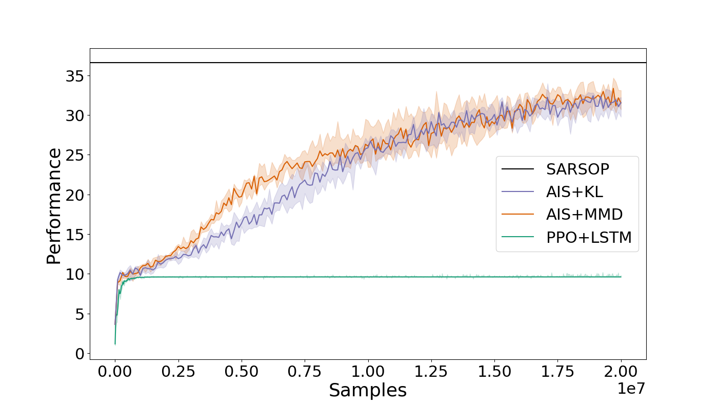
(a) Rock Sampling

(b) Drone Surveillance

Figure 6: Comparison of AIS-based actor only PORL algorithm with LSTM+PPO baseline for moderate-dimensional environments (for 10 random seeds).

In these environments, the size of the unobserved state is moderately large (of the order of $10^{2}$ to $10^{3}$ unobserved states) and the optimal planning solution cannot be easily obtained using standard POMDP solvers. However, an approximate planning solution can be easily obtained using standard approximation algorithms for POMDPs.

1. 

   RockSample: RockSample is a scalable POMDP environment introduced in Smith and Simmons (2004) which models the rover science exploration. The RockSample$(n,k)$ environment consists of a $n\times n$ grid with $k$ rocks. The rocks are at known positions. Some of the rocks which are labeled as good rocks have scientific values; other rocks which are labeled as bad rocks do not. Sampling a rock is expensive and the agent has a noisy long-range sensor to help determine if a rock is good before choosing to approach and sample it. At each stage, the agent can choose from $k+5$ actions: north, south, east, west, sample, check₁, …, check_$k$. The first four are deterministic single-step motion actions. The sample action samples the rock at the current location; if the rock is good, there is a reward of $+20$ and the rock becomes bad (so that no further reward can be gained from sampling it); if the rock is bad, there is a negative reward of $-10$. The right edge of the map is a terminal state and reaching it gives a reward of $+10$. In our experiments, we use a RockSample$(5,3)$ environment.

2. 

   DroneSurveillance: DroneSurveillance is a POMDP model of deploying an autonomous aerial vehicle in a partially observed, dynamic, indoor environment introduced in Svoreňová et al. (2015). The environment is a $5\times 5$ grid with two agents: a ground agent which moves randomly and an aerial agent, whose motion has to be controlled. The aerial agent starts at the bottom-left cell and has to reach the upper-right cell (the goal state) without being in the same location as the ground agent. The ground agent cannot enter the start or goal states. The aerial agent has a downward facing camera which can view a $3\times 3$ grid centered at its current location and it can perfectly see the location of the ground agent if it is in this view. At each stage, the aerial agent may choose from $5$ actions: north, south, east, west, hover. The first four are deterministic single-step motion actions and the hover action keeps the aerial vehicle at its current position. Reaching the goal gives a reward of $+1$ and ends the episode. If both agents are in the same cell, there is a negative reward of $-1$ and the episode ends.

The visualizations above are taken from the JuliaPOMDP environments (Egorov et al., 2017). For both environments, we compare the performance of AIS-based PORL with the LSTM+PPO baseline described earlier. We also compare with the best performing planning solution from the JuliaPOMDP repository (Egorov et al., 2017). The results are shown in Fig. 6 which shows that both AIS-based PORL algorithms converge close to the best planning solution in both environments. The performance of LSTM+PPO is similar in DroneSurveillance but LSTM+PPO gets stuck in a local minima in RockSample.

7.3 High-dimensional environments

We use the MiniGrid environments from the BabyAI platform (Chevalier-Boisvert et al., 2018b), which are partially observable 2D grid environments which has tasks of increasing complexity level. The environment has multiple entities (agent, walls, lava, boxes, doors, and keys); objects can be picked up, dropped, and moved around by the agent; doors can be unlocked via keys of the same color (which might be hidden inside boxes). The agents can see a $7\times 7$ view in front of it but it cannot see past walls and closed doors. At each time, it can choose from the following actions: $\{$Move Forward, Turn Left, Turn Right, Open Door/Box, Pick up item, Drop Item, Done$\}$. The agent can only hold one item at a time. The objective is to reach a goal state in the quickest amount of time (which is captured by assigning to the goal state a reward which decays over time).

Most of the environments have a certain theme, and we cluster the environments accordingly. The visualizations below are taken from the Gym Minigrid environments (Chevalier-Boisvert et al., 2018b).

1. 

   Simple Crossing: A simple crossing environment is a 2D grid with columns of walls with an opening (or a crossing). The agent can traverse the wall only through the openings and needs to find a path from the start to the goal state. There are four such environments (MGSCS9N1, MGSCS9N2, MGSCS9N3, and MGSCS11N5) where the label S$n$N$m$ means that the size of the environment is $n\times n$ and there are $m$ columns of walls.

2. 

   Lava Crossing: The lava crossing environments are similar to the simple crossing environments, but the walls are replaced by lava. If the agent steps on to the lava block then it dies and the episode ends. Therefore, exploration is more difficult in lava crossing as compared to simple crossing. There are two such environments (MGLCS9N1 and MGLCS9N2) where the label S$n$N$m$ has the same interpretation as simple crossing.

3. 

   Key Corridor: The key corridor environments consist of a central corridor which has rooms on the left and right sides which can be accessed through doors. When the door is locked it can be opened using a key of the same color. The agent has to move to the location of the key, pick it up, move to the location of the correct door, open the door, drop the key, and pick up the colored ball. There are three such environments (MGKCS3R1, MGKCS3R2, and MGKCS3R3), where the label S$n$R$m$ means that the size of the grid is proportional to $n$ and the number of rooms present is $2m$.

4. 

   Obstructed Maze: The obstructed maze environments are similar to key corridor environments but the key is inside a box and the box has to be opened to find the key. We consider two such environments (MGOM1Dl and MGOM1Dlh). In MGOM1Dl box is already open while in MGOM1Dlh the box is closed. There is an additional such environment in the BabyAI platform (MGOM1Dlhb), which is more suitable for continual learning algorithms so we exclude it here.

The number of observations in a given Minigrid environment is discrete but is too large to model it as a one-hot encoded discrete observation as done in the previous environments. Instead we compress the observations as described in Section 3.7 by using an autoencoder to convert a large discrete space to a continuous space with a tractable size. A separate autoencoder is trained for each environment using a dataset that is created by performing random rollouts. Once the autoencoder is trained over the fixed dataset for several epochs, it is fixed and used to generate the observations for learning the AIS. This is very similar to Ha and Schmidhuber (2018), where they learn the autoencoder in a similar fashion and then fix it, following which their training procedure for the next observation distribution prediction and policy takes place.

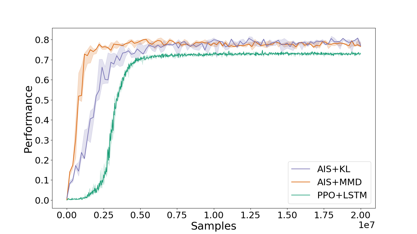
(a) MGSCS9N1

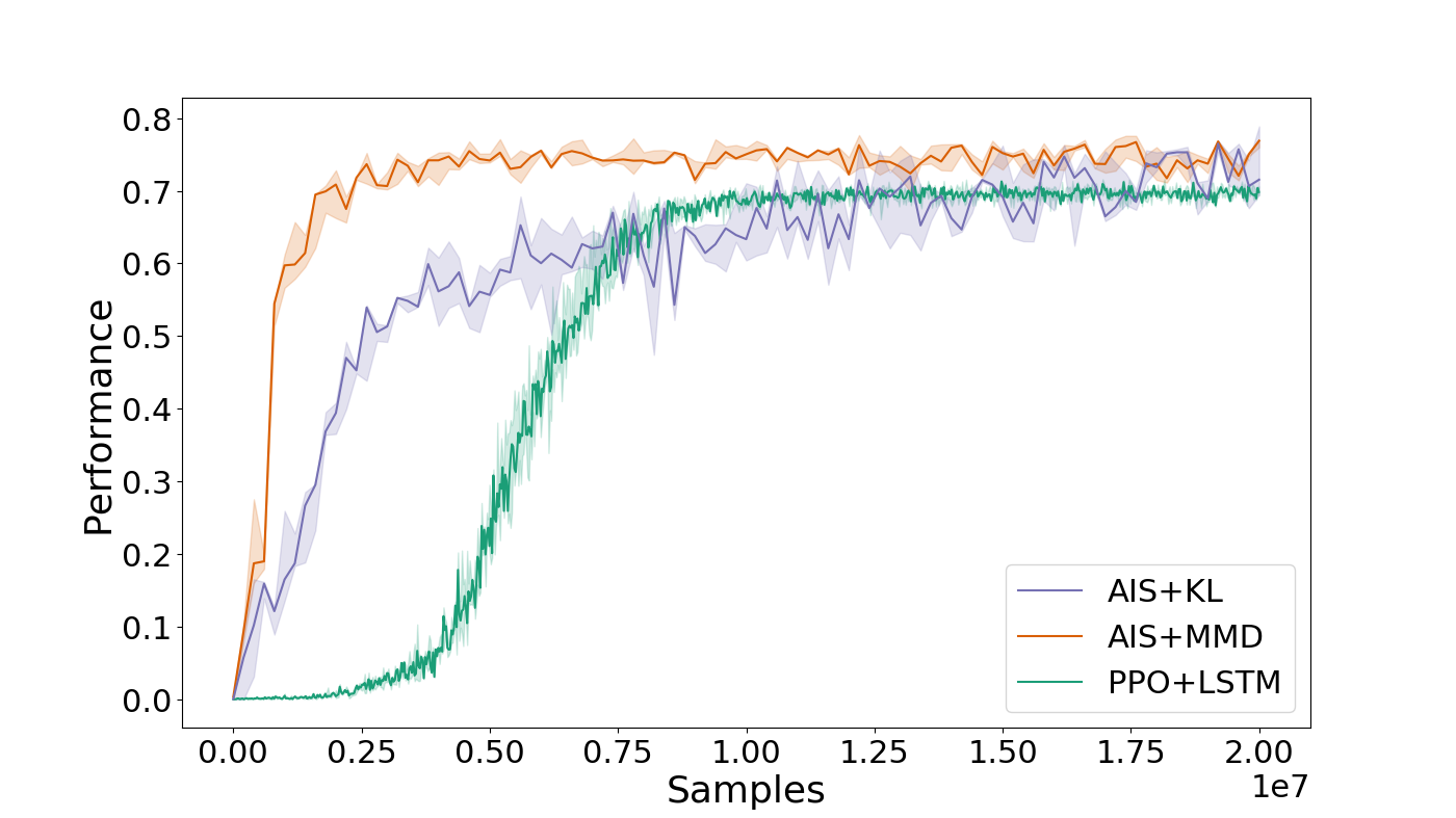
(b) MGSCS9N2

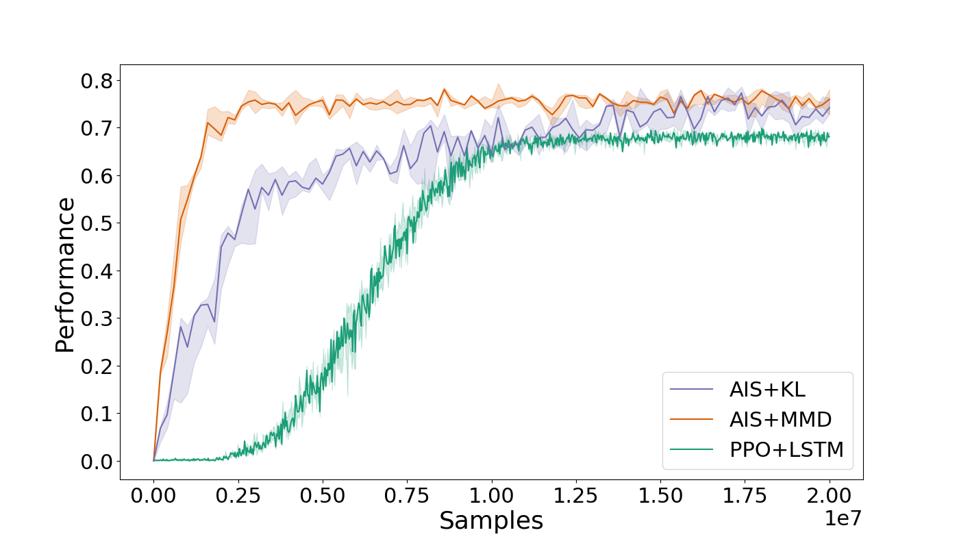
(c) MGSCS9N3

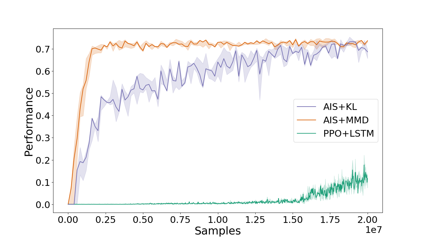
(d) MGSCS11N5

(e) MGLCS9N1

(f) MGLCS9N2

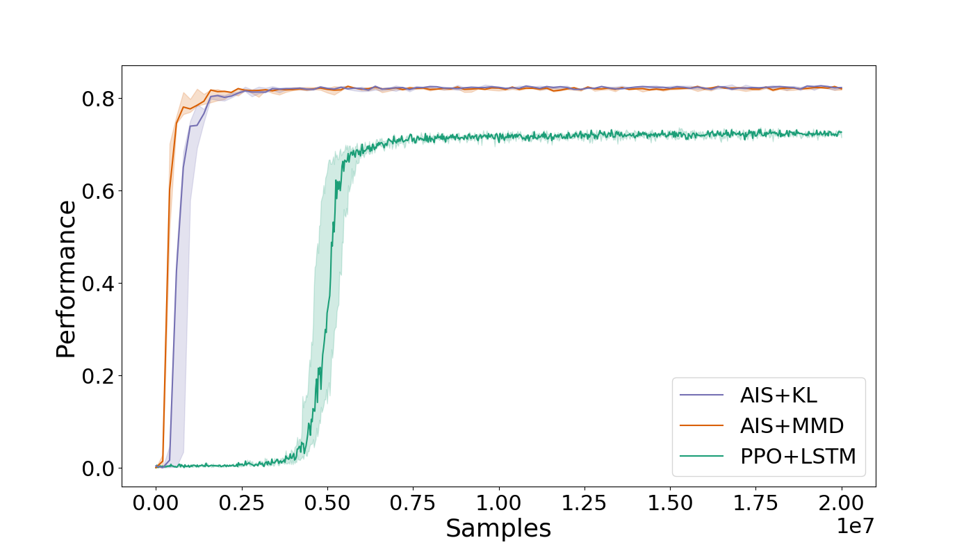
(g) MGKCS3R1

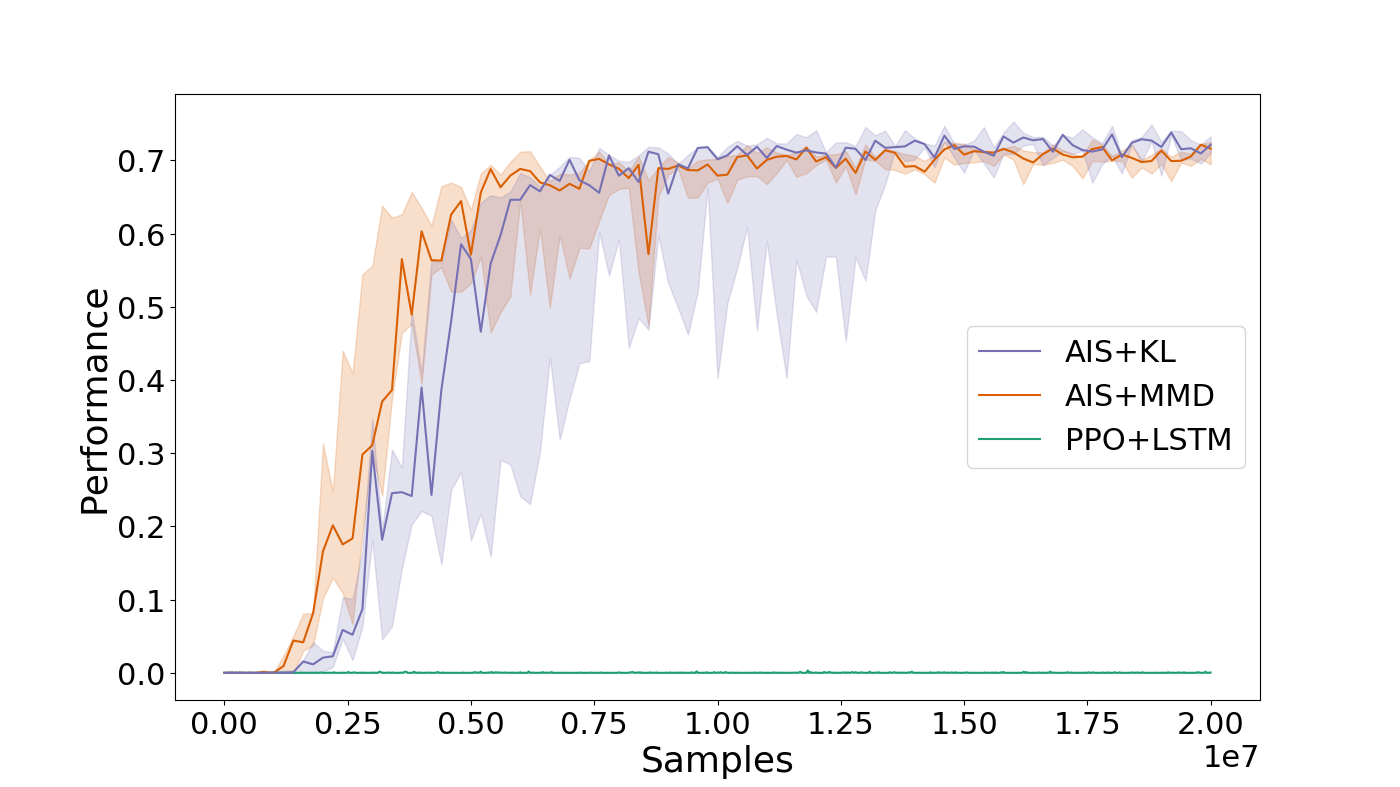
(h) MGKCS3R2

Figure 7: Comparison of AIS-based actor only PORL algorithm with LSTM+PPO baseline for high-dimensional environments (for 5 random seeds).

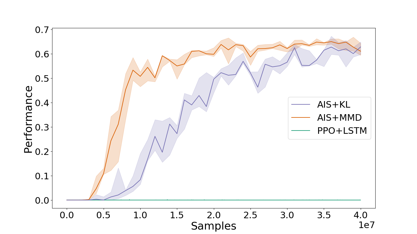
(a) MGKCS3R3

(b) MGOM1Dl

(c) MGOM1Dlh

Figure 7 (continued): Comparison of AIS-based actor only PORL algorithm with LSTM+PPO baseline for high-dimensional environments (for 5 random seeds).

Note that the output of the autoencoder is a continuous variable and we are using MMD with $p=2$ as an IPM. As explained in Section 6.1, $d_{\mathfrak{F}_{2}}(\mu,\nu)^{2}$ only depends on the mean of $\mu$ and $\nu$. So, to simplify the computations, we assume that $\nu$ is a Dirac delta distribution centered at its mean. Thus, effectively, we are predicting the mean of the next observation. In general, simply predicting the mean of the observations may not lead to a good representation, but in the Minigrid environments, the transitions are deterministic and the only source of stochasticity in the observations is due to the initial configuration of the environment. So, in practice, simply predicting the mean of the next observation works reasonably well. We emphasize that for other more general environments with truly stochastic observations, such a choice of IPM may not work well and it may be better to choose the MMD $d_{\mathfrak{F}_{p}}$ defined in Proposition 32 for a different value of $p$, say $p=1$ (which corresponds to the energy distance (Székely and Rizzo, 2004)).

For all minigrid environments, we compare the performance of AIS-based PORL with the LSTM+PPO baseline proposed in Chevalier-Boisvert et al. (2018a). The results are shown in Fig. 7 which shows that for most environments AIS-based PORL converges to better performance values. Note that AIS-based PORL fails to learn in the Lava Crossing environments (MGLCS9N1 and MGLCS9N2) while LSTM+PPO fails to learn in the larger Key Crossing environments (MGKCS3R2 and MGKCS3R3) and in the Obstructed Maze environments (MGOM1Dl and MGOM1Dlh).

The results indicate that one IPM does not necessarily lead to better performance than others in all cases. The performance of a particular IPM depends on whether the observation and AIS spaces are discrete or continuous, on the size of these spaces, and the stochasticity of the environment. The fact that we are approximating the policy using non-linear neural networks makes it difficult to quantify the impact of the choice of IPM on the accuracy of learning. It will be important to understand this impact in more detail and develop guidelines on how to choose an IPM based on the features of the environment.

8 Conclusion

In this paper, we present a theoretical framework for approximate planning and learning in partially observed system. Our framework is based on the fundamental notion of information state. We provide two equivalent definitions of information state. An information state is a function of history which is sufficient to compute the expected reward and predict its next value. Equivalently, an information state is a function of the history which can be recursively updated and is sufficient to compute the expected reward and predict the next observation. We show that an information state always leads to a dynamic programming decomposition and provide several examples of simplified dynamic programming decompositions proposed in the literature which may be viewed as specific instances of information states.

We then relax the definition of an information state to describe an approximate information state (AIS), which is a function of the history that approximately satisfies the properties of the information state. We show that an AIS can be used to identify an approximately optimal policy with the approximation error specified in terms of the “one-step” approximation errors in the definition of the AIS. We present generalizations of AIS to setups with observation and action compression as well as to multi-agent systems. We show that various approximation approaches for both fully and partially observed setups proposed in the literature may be viewed as special cases of AIS.

One of the salient features of the AIS is that it is defined in terms of properties that can be estimated from data, and hence the corresponding AIS generators can be learnt from data. These can then be used as history representations in partially observed reinforcement learning (PORL) algorithms. We build up on this idea to present policy gradient algorithms which learn an AIS representation and an optimal policy and/or action-value function using multi time-scale stochastic gradient descent.

We present detailed numerical experiments which compare the performance of AIS-based PORL algorithms with a state-of-the-art PORL algorithm for three classes of partially observed problems—small, medium and large scale problems—and find out that AIS-based PORL outperforms the state-of-the-art baseline in most cases.

We conclude by observing that in this paper we restricted attention to the simplest classes of algorithms but the same idea can be extended to develop AIS-based PORL algorithms which uses value-based approaches such as Q-learning and its improved variants such as DQN, DDQN, distributional RL, etc. Finally, we note that the AIS representation includes a model of the system, so it can be used as a component of model-based reinforcement learning algorithms such as Dyna (Sutton and Barto, 2018, Sec 8.2, page 161). Such an approach will provide anytime guarantees on the approximation error which will depend on the “one-step” approximation error of the current AIS-representation. Therefore, we believe that AIS presents a systematic framework to reason about learning in partially observed environments.

Appendix A Comparison with the results of Abel et al. (2016) for state aggregation in MDPs

Abel et al. (2016) introduce four models of state aggregation and derive approximation bounds for all four. In this section, we show that one of these models, which they call approximate model similarity may be viewed as an AIS. We also show that the approximation bounds of Theorem 27 for this model are stronger than those derived in Abel et al. (2016) by a factor of $\mathcal{O}(1/(1-\gamma))$.

Since we follow a slightly different notation than Abel et al. (2016) and for the sake of completeness, we start by describing the notion of approximate model similarity defined in Abel et al. (2016).

Consider an infinite horizon finite-state finite-action MDP with state space $\mathsf{S}$, action space $\mathsf{A}$, transition probability matrix $P\colon\mathsf{S}\times\mathsf{A}\to\Delta(\mathsf{S})$, per-step reward function $r\colon\mathsf{S}\times\mathsf{A}\to\mathbb{R}$, and discount factor $\gamma$.

Let $\hat{\mathsf{S}}$ be an aggregated state space and it is assumed that the following two functions are available: a compression function $q\colon\mathsf{S}\to\hat{\mathsf{S}}$ and a weight function $w\colon\mathsf{S}\to[0,1]$ such that for all $\hat{s}\in\hat{\mathsf{S}}$, $\sum_{s\in q^{-1}(\hat{s})}w(s)=1$. Given these functions, define an aggregated MDP with state space $\hat{\mathsf{S}}$, action space $\mathsf{A}$, transition probability function $\hat{P}\colon\hat{\mathsf{S}}\times\mathsf{A}\to\hat{\mathsf{S}}$ given by

$$\hat{P}(\hat{s}^{\prime}|\hat{s},a)=\sum_{s\in q^{-1}(\hat{s})}\sum_{s^{\prime}\in q^{-1}(\hat{s}^{\prime})}P(s^{\prime}|s,a)w(s),\quad\forall\hat{s},\hat{s}^{\prime}\in\hat{\mathsf{S}},a\in\mathsf{A},$$

and a per-step reward $\hat{r}\colon\hat{\mathsf{S}}\times\mathsf{A}\to\mathbb{R}$ given by

$$\hat{r}(\hat{s},a)=\sum_{s\in q^{-1}(\hat{s})}r(s,a)w(s),\quad\forall\hat{s}\in\hat{\mathsf{S}},a\in\mathsf{A}.$$

Definition 34 ($\varepsilon$-approximate model similarity (Abel et al., 2016))

The aggregated MDP is said to be $\varepsilon$-approximate model similar to the original MDP if it satisfies the following two properties:

1. For all $\hat{s}\in\hat{\mathsf{S}}$, $s_{1},s_{2}\in q^{-1}(\hat{s})$, and $a\in\mathsf{A}$, we have

   $$\bigl{|}r(s_{1},a)-r(s_{2},a)\bigr{|}\leq\varepsilon.$$

2. For all $\hat{s},\hat{s}^{\prime}\in\hat{\mathsf{S}}$, $s_{1},s_{2}\in q^{-1}(\hat{s})$, and $a\in\mathsf{A}$, we have

   $$\biggl{|}\sum_{s^{\prime}\in q^{-1}(\hat{s}^{\prime})}P(s^{\prime}|s_{1},a)-\sum_{s^{\prime}\in q^{-1}(\hat{s}^{\prime})}P(s^{\prime}|s_{2},a)\biggr{|}\leq\varepsilon.$$

Proposition 35 (Lemma 2 of Abel et al. (2016))

Let $\hat{\pi}\colon\hat{\mathsf{S}}\to\mathsf{A}$ be the (deterministic) optimal policy for the aggregated MDP. Define $\pi\colon\mathsf{S}\to\mathsf{A}$ by $\pi=\hat{\pi}\circ q$. Let $V\colon\mathsf{S}\to\mathbb{R}$ denote the optimal value function and let $V^{\pi}\colon\mathsf{S}\to\mathbb{R}$ denote the value function for policy $\pi$. Then, for all $s\in\mathsf{S}$

$$\bigl{|}V(s)-V^{\pi}(s)\bigr{|}\leq\frac{2\varepsilon}{(1-\gamma)^{2}}+\frac{2\gamma\varepsilon|\mathsf{S}|\|r\|_{\infty}}{(1-\gamma)^{3}}.$$

Note that the result is presented slightly differently in Abel et al. (2016). They assume that $\|r\|_{\infty}=1$ and simplify the above expression.

We now show an approximate model similarity is also an AIS and directly using the result of Theorem 27 for this model gives a stronger bound than Proposition 35.

Proposition 36

Let $(q,w)$ be such that the aggregated model is $\varepsilon$-approximate model similar to the true model. Then, $(q,\hat{P},\hat{r})$ is an $(\varepsilon,\varepsilon|\hat{\mathsf{S}}|)$-AIS with respect to the total variation distance.

Proof  We first establish (AP1). For any $s\in\mathsf{S}$ and $a\in\mathsf{A}$,

$$\bigl{|}r(s,a)-\hat{r}(q(s),a)\bigr{|} \stackrel{{\scriptstyle(a)}}{{\leq}}\biggl{|}\sum_{\tilde{s}\in q^{-1}(q(s))}w(\tilde{s})r(s,a)-\sum_{\tilde{s}\in q^{-1}(q(s))}w(\tilde{s})r(\tilde{s},a)\biggr{|}$$

$$\stackrel{{\scriptstyle(b)}}{{\leq}}\sum_{\tilde{s}\in q^{-1}(q(s))}w(\tilde{s})\bigl{|}r(s,a)-r(\tilde{s},a)\bigr{|}$$

$$\stackrel{{\scriptstyle(c)}}{{\leq}}\varepsilon$$

where $(a)$ follows from the basic property of the weight function $w$ and the definition of the aggregated reward $\hat{r}$; $(b)$ follows form the triangle inequality; and $(c)$ follows from the definition of approximate model similarity and the basic property of the weight function $w$. This establishes property (AP1).

Now, we establish (AP2). Let $d_{\mathfrak{F}}$ denote the total variation distance. Define probability measures $\mu,\nu$ on $\Delta(\hat{\mathsf{S}})$ in the definition of (AP2), i.e., for any $s\in\mathsf{S}$, $\hat{s}^{\prime}\in\hat{\mathsf{S}}$, and $a\in\mathsf{A}$,

$$\mu(\hat{s}^{\prime}) \coloneqq\sum_{s^{\prime}\in q^{-1}(\hat{s}^{\prime})}P(s^{\prime}|s,a)$$

$$\nu(\hat{s}^{\prime}) \coloneqq\hat{P}(\hat{s}^{\prime}|q(s),a)=\sum_{\tilde{s}\in q^{-1}(q(s))}\sum_{s^{\prime}\in q^{-1}(\hat{s}^{\prime})}P(s^{\prime}|\tilde{s},a)w(\tilde{s})$$

Now consider (see footnote 1 on page 1)

$$d_{\mathfrak{F}}(\mu,\nu) =\sum_{\hat{s}^{\prime}\in\hat{\mathsf{S}}}|\mu(\hat{s}^{\prime})-\nu(\hat{s}^{\prime})|$$

$$=\sum_{\hat{s}^{\prime}\in\hat{\mathsf{S}}}\biggl{|}\sum_{s^{\prime}\in q^{-1}(\hat{s}^{\prime})}P(s^{\prime}|s,a)-\sum_{\tilde{s}\in q^{-1}(q(s))}\sum_{s^{\prime}\in q^{-1}(\hat{s}^{\prime})}P(s^{\prime}|\tilde{s},a)w(\tilde{s})\biggr{|}$$

$$\stackrel{{\scriptstyle(a)}}{{\leq}}\sum_{\hat{s}^{\prime}\in\hat{\mathsf{S}}}\sum_{\tilde{s}\in q^{-1}(q(s))}w(\tilde{s})\biggl{|}\sum_{s^{\prime}\in q^{-1}(\hat{s}^{\prime})}P(s^{\prime}|s,a)-\sum_{s^{\prime}\in q^{-1}(\hat{s}^{\prime})}P(s^{\prime}|\tilde{s},a)\biggr{|}$$

$$\stackrel{{\scriptstyle(b)}}{{\leq}}\sum_{\hat{s}^{\prime}\in\hat{\mathsf{S}}}\sum_{\tilde{s}\in q^{-1}(q(s))}w(\tilde{s})\varepsilon\stackrel{{\scriptstyle(c)}}{{=}}\sum_{\hat{s}^{\prime}\in\hat{\mathsf{S}}}\varepsilon=|\hat{\mathsf{S}}|\varepsilon,$$

where $(a)$ follows from triangle inequality, $(b)$ follows from definition of approximate model similarity and $(c)$ follows from the basic property of the weight function. This proves (AP2).  

Lemma 37

For any MDP

$$\operatorname{span}(V)\leq\frac{\operatorname{span}(r)}{1-\gamma}.$$

Therefore, when $d_{\mathfrak{F}}$ is the total variation distance, $\rho_{\mathfrak{F}}(V)\leq\tfrac{1}{2}\operatorname{span}(r)/(1-\gamma)$.

Proof  This result follows immediately by observing that the per-step cost $r(S_{t},A_{t})\in[\min(r),\max(r)]$. Therefore, $\max(V)\leq\max(r)/(1-\gamma)$ and $\min(V)\geq\min(r)/(1-\gamma)$.  

Proposition 38

Let $\hat{\pi}$, $\pi$, $V$, and $V^{\pi}$ be defined as in Proposition 36. Then, for all $s\in\mathsf{S}$,

$$\bigl{|}V(s)-V^{\pi}(s)\bigr{|}\leq\frac{2\varepsilon}{(1-\gamma)}+\frac{\gamma\varepsilon|\hat{\mathsf{S}}|\operatorname{span}(r)}{(1-\gamma)^{2}}.$$

Proof  This follows immediately from Theorem 27, Proposition 36 and Lemma 37.  

Note that the error bounds of Propositions 36 and 38 have similar structure but the key difference is that the bound of Proposition 38 is tighter than a factor of $1/(1-\gamma)$ as compared to Proposition 36. There are other minor improvements as well ($|\hat{\mathsf{S}}|$ instead of $|\mathsf{S}|$ and $\tfrac{1}{2}\operatorname{span}(r)$ instead of $\|r\|_{\infty}$).

Appendix B Comparison with the results of Gelada et al. (2019) for latent space models for MDPs

Gelada et al. (2019) propose a latent space model for an MDP and show that minimizing the losses in predicting the per-step reward and repredicting the distribution over next latent space provides a bound on the quality of the representation. In this section, we show that latent space representation defined in Gelada et al. (2019) may be viewed as an instance of an AIS and show that the approximation bounds of Theorem 27 are similar to those derived in Gelada et al. (2019).

Since we follow a slightly different notation than Gelada et al. (2019) and for the sake of completeness, we start by describing the notion of latent space representation used in Gelada et al. (2019).

Consider an MDP with infinite horizon, finite-state and finite-action having state space $\mathsf{S}$, action space $\mathsf{A}$, transition probability matrix $P\colon\mathsf{S}\times\mathsf{A}\to\Delta(\mathsf{S})$, per-step reward function $r\colon\mathsf{S}\times\mathsf{A}\to\mathbb{R}$ and discount factor $\gamma$.

Let $(\hat{\mathsf{S}},d)$ be a Banach space and it is assumed that we are given an embedding function $\phi\colon\mathsf{S}\to\hat{\mathsf{S}}$, along with transition dynamics $\hat{P}\colon\hat{\mathsf{S}}\times\mathsf{A}\to\Delta(\hat{\mathsf{S}})$ and reward function $\hat{r}\colon\hat{\mathsf{S}}\times\mathsf{A}\to\mathbb{R}$. The MDP $\widehat{\mathcal{M}}=(\hat{\mathsf{S}},\mathsf{A},\hat{P},\hat{r},\gamma)$ along with the embedding function $\phi$ is called the latent space model of the original MDP.

Definition 39

The MDP $\widehat{\mathcal{M}}$ is said to be $(L_{r},L_{p})$-Lipschitz if for any $\hat{s}_{1},\hat{s}_{2}\in\hat{\mathsf{S}}$ and $a\in A$,

$$\bigl{|}\hat{r}(\hat{s}_{1},a)-\hat{r}(\hat{s}_{2},a)\bigr{|}\leq L_{r}d(\hat{s}_{1},\hat{s}_{2})\quad\text{and}\quad d_{\mathfrak{F}}(\hat{P}(\cdot|\hat{s}_{1},a),\hat{P}(\cdot|\hat{s}_{2},a))\leq L_{p}d(\hat{s}_{1},\hat{s}_{2}),$$

where $d_{\mathfrak{F}}$ denotes the Kantorovich distance.

Given a latent space embedding, define

$$\varepsilon=\sup_{s\in\mathsf{S},a\in\mathsf{A}}\bigl{|}r(s,a)-\hat{r}(\phi(s),a)\bigr{|}\quad\text{and}\quad\delta=\sup_{s\in\mathsf{S},a\in\mathsf{A}}d_{\mathfrak{F}}(\mu,\hat{P}(\cdot|\phi(s),a)),$$

where $\mu\in\Delta(\hat{\mathsf{S}})$ given by $\mu(\mathsf{B})=P(\phi^{-1}(\mathsf{B})|s,a)$ for any Borel subset $\mathsf{B}$ of $\hat{\mathsf{S}}$.

Proposition 40 (Theorem 5 of Gelada et al. (2019))

Let $\hat{\pi}\colon\hat{\mathsf{S}}\to\mathsf{A}$ be the (deterministic) optimal policy of the latent space MDP. Define $\pi\colon\mathsf{S}\to\mathsf{A}$ by $\pi=\hat{\pi}\circ\phi$. Let $V\colon\mathsf{S}\to\mathbb{R}$ denote the optimal value function and let $V^{\pi}\colon\mathsf{S}\to\mathbb{R}$ denote the value function for policy $\pi$.

If the latent space MDP $\widehat{\mathcal{M}}$ is $(L_{r},L_{p})$-Lipschitz, then,

$$\bigl{|}V(s)-V^{\pi}(s)\bigr{|}\leq\frac{2\varepsilon}{1-\gamma}+\frac{2\gamma\delta L_{r}}{(1-\gamma)(1-\gamma L_{p})}.$$

We show that a latent space model is an AIS and directly using the result of Theorem 27 gives the same approximation bound.

Proposition 41

Let $\widehat{\mathcal{M}}=(\hat{\mathsf{S}},\mathsf{A},\hat{P},\hat{r},\gamma)$ be a latent space model with embedding function $\phi$. Then, $(\phi,\hat{P},\hat{r})$ is an $(\varepsilon,\delta)$-AIS with respect to the Kantorovich distance.

Proof  The result is an immediate consequence of the definition of $\varepsilon$ and $\delta$ for latent space model.  

Lemma 42

For any $(L_{r},L_{p})$-Lipschitz MDP, if $\gamma L_{p}<1$, then

$$\|V\|_{\mathrm{Lip}}\leq\frac{L_{r}}{1-\gamma L_{p}}.$$

Therefore, when $d_{\mathfrak{F}}$ is the Kantorovich distance, $\rho_{\mathfrak{F}}(V)=\|V\|_{\mathrm{Lip}}\leq L_{r}/(1-\gamma L_{p})$.

Proof  This result follows immediately from Theorem 4.2 of Hinderer (2005).  

Proposition 43

Let $\hat{\pi}$, $\pi$, $V$, and $V^{\pi}$ be defined in Proposition 40. The, for all $s\in\mathsf{S}$,

$$\bigl{|}V(s)-V^{\pi}(s)\bigr{|}\leq\frac{2\varepsilon}{1-\gamma}+\frac{2\gamma\delta L_{r}}{(1-\gamma)(1-\gamma L_{p})}.$$

Proof  This follows immediately from Theorem 27, Proposition 40, and Lemma 42.  

Note that the error bounds in Propositions 40 and 43 are exactly the same.

Appendix C Comparison with the results of Francois-Lavet et al. (2019) for belief approximation in POMDPs

Francois-Lavet et al. (2019) analyze the trade off between asymptotic bias and overfitting in reinforcement learning with partial observations. As part of their analysis, they express the quality of state representation in terms of the bounds on the $L_{1}$ error of the associated belief states. We show that these approximation bounds may be viewed as an instance of AIS-based bounds of Theorems 9 and 27. We also show that the bounds of Theorem 27 for this model are stronger than those derived in Francois-Lavet et al. (2019) by a factor of $\mathcal{O}(1/(1-\gamma))$.

Since we follow a slightly different notation than Francois-Lavet et al. (2019) and for the sake of completeness, we start by describing the notion of $\varepsilon$-sufficient statistics defined in Francois-Lavet et al. (2019).

Consider an infinite-horizon finite-state finite-action POMDP with state space $\mathsf{S}$, action space $\mathsf{A}$, observation space $\mathsf{Y}$, transition probability matrix $P\colon\mathsf{S}\times\mathsf{A}\to\Delta(\mathsf{S})$, observation matrix $P^{y}\colon\mathsf{S}\to\Delta(\mathsf{Y})$, per-step reward $r\colon\mathsf{S}\times\mathsf{A}\to\mathbb{R}$, and discount factor $\gamma$.

Definition 44 ($\varepsilon$-sufficient statistic (Francois-Lavet et al., 2019))

Given a family of Banach spaces $\{\Phi_{t}\}_{t=1}^{L}$, an $\varepsilon$-sufficient statistic is a collection of history compression function $\{\phi_{t}\colon\mathsf{H}_{t}\to\Phi_{t}\}_{t=1}^{T}$ and belief approximation functions $\{\hat{b}_{t}\colon\Phi_{t}\to\Delta(\mathsf{S})\}_{t=1}^{T}$ such that for any time $t$ and any realization $h_{t}$ of $H_{t}$, we have

$$\|\hat{b}_{t}(\cdot|\phi_{t}(h_{t}))-b_{t}(\cdot|h_{t})\|_{1}\leq\varepsilon.$$

Given an $\varepsilon$-sufficient statistic, Francois-Lavet et al. (2019) define an MDP with state space $\Delta(\mathsf{S})$, action space $\mathsf{A}$, transition probability kernel $\mathbb{P}(\hat{b}_{t+1}(\cdot|\phi(h_{t+1}))\mid\hat{b}_{t}(\cdot|\phi(h_{t})),a_{t})$ computed from the underlying POMDP, and per-step reward given by

$$\hat{r}(\hat{b}_{t}(h_{t}),a_{t})=\sum_{s\in\mathsf{S}}r(s,a_{t})\hat{b}_{t}(s|\phi(h_{t})).$$

Proposition 45 (Theorem 1 of Francois-Lavet et al. (2019))

Let $\{(\hat{b}_{t},\phi_{t})\}_{t=1}^{T}$ be an $\varepsilon$-sufficient statistic and $\hat{\pi}=(\hat{\pi}_{1},\hat{\pi}_{2},\dots)$ be an optimal policy for the MDP described above. Define a policy $\pi=(\pi_{1},\pi_{2},\dots)$ given by $\pi_{t}=\hat{\pi}_{t}\circ\phi_{t}$. Let $V_{t}\colon\mathsf{H}_{t}\to\mathbb{R}$ denote the optimal value functions and $\hat{V}^{\pi}_{t}\colon H_{t}\to\mathbb{R}$ denote the value function for policy $\pi$. Then for any initial history $h_{1}\in\mathsf{H}_{1}$,

$$\bigl{|}V_{1}(h_{1})-V_{1}^{\pi}(h_{1})\bigr{|}\leq\frac{2\varepsilon\|r\|_{\infty}}{(1-\gamma)^{3}}.$$

We now show that an $\varepsilon$-sufficient statistic gives rise to an AIS and directly using the results of Theorem 27 for this model gives a stronger bound than Proposition 45.

Proposition 46

Let $\{(\hat{b}_{t},\phi_{t})\}_{t=1}^{T}$ be an $\varepsilon$-sufficient statistic. Let $\hat{\mathsf{Z}}_{t}=\Delta(\mathsf{S})$ and define the different components of an AIS as follows:

• history compression functions $\hat{\sigma}_{t}=\hat{b}_{t}\circ\phi_{t}$,

• AIS prediction kernels $\hat{P}_{t}(\cdot|\hat{z}_{t},a_{t})$ is given by

  $$\hat{P}_{t}(\mathsf{B}|\hat{z}_{t},a_{t})=\sum_{y_{t+1}\in\mathsf{Y}}\psi(y_{t+1}|\hat{z}_{t},a_{t})\mathds{1}_{\mathsf{B}}\{\hat{\varphi}(\hat{z}_{t},y_{t+1},a_{t})\},$$

  where

  $$\psi(y_{t+1}|\hat{z}_{t},a_{t})=\sum_{s_{t+1}\in\mathsf{S}}\sum_{s_{t}\in\mathsf{S}}P^{y}(y_{t+1}|s_{t+1})P(s_{t+1}|s_{t},a_{t})\hat{z}_{t}(s_{t})$$

  and

  $$\hat{\varphi}(\hat{z}_{t},y_{t+1},a_{t})(s_{t+1})=\frac{\sum_{s_{t}\in\mathsf{S}}P^{y}(y_{t+1}|s_{t+1})P(s_{t+1}|s_{t},a_{t})\hat{z}_{t}(s_{t})}{\psi(y_{t+1}|\hat{z}_{t},a_{t})},$$

  where $\hat{\varphi}$ is the same as the Bayes’-rule based update of the belief state,

• reward approximation functions $\hat{r}(\hat{z}_{t},a_{t})=\sum_{s\in S}\hat{z}_{t}(s)r(s,a_{t})$.

Then, $\{(\hat{\sigma}_{t},\hat{P}_{t},\hat{r}_{t})\}_{t=1}^{T}$ is an $(\varepsilon\|r\|_{\infty},3\varepsilon)$-AIS with respect to the bounded-Lipschitz metric.

Proof  We need to equip $\hat{\mathsf{Z}}=\Delta(\mathsf{S})$ with a metric in order to define a bounded-Lipschitz metric over $\Delta(\hat{\mathsf{Z}})$. We use the total variation as the metric and denote it by $d_{\mathrm{TV}}$. We use $\mathfrak{F}$ to denote $\{f\colon\Delta(\hat{\mathsf{Z}})\to\mathbb{R}:\|f\|_{\infty}+\|f\|_{\mathrm{Lip}}\leq 1\}$ and denote the corresponding bounded-Lipschitz metric over $\Delta(\hat{\mathsf{Z}})$ by $d_{\mathfrak{F}}$.

We first establish (AP1). For any time $t$, realization $h_{t}$ of history $H_{t}$, and action $a_{t}\in\mathsf{A}$, we have

$$\bigl{|}\mathbb{E}[r(S_{t},a_{t}) \mid H_{t}=h_{t},A_{t}=a_{t}]-\hat{r}_{t}(\hat{\sigma}_{t}(h_{t}),a_{t})\bigr{|}$$

$$=\biggl{|}\sum_{s\in\mathsf{S}}r(s,a_{t})b_{t}(s|h_{t})-\sum_{s\in\mathsf{S}}r(s,a_{t})\hat{b}_{t}(s|\phi(h_{t}))\biggr{|}$$

$$\stackrel{{\scriptstyle(a)}}{{\leq}}\|r\|_{\infty}d_{\mathrm{TV}}(b_{t},\hat{b}_{t})$$

$$\stackrel{{\scriptstyle(b)}}{{\leq}}\varepsilon\|r\|_{\infty}$$

where $(a)$ follows from (10) and the fact that for total variation distance $\rho_{\mathrm{TV}}(r)\leq\|r\|_{\infty}$; and $(b)$ follows from definition of $\varepsilon$-sufficient statistic.

Before establishing (AP2), we note that $\hat{\varphi}$ is the Bayes’-rule based update of the true belief; therefore,

$$b_{t+1}(\cdot|h_{t+1})=\hat{\varphi}(b_{t}(\cdot|h_{t}),y_{t+1},a_{t}).$$

For ease of notation, we use $b_{t}(\cdot)$ and $\hat{b}_{t}(\cdot)$ instead of $b_{t}(\cdot|h_{t})$ and $\hat{b}_{t}(\cdot|\phi_{t}(h_{t}))$, when the conditioning is clear from context.

Now consider $\mu_{t}$ and $\nu_{t}$ as defined in the definition of (AP2). In particular, for any Borel set $\mathsf{B}$,

$$\mu_{t}(\mathsf{B}) =\sum_{y_{t+1}\in\mathsf{Y}}\psi(y_{t+1}|b_{t},a_{t})\mathds{1}_{\mathsf{B}}\{\hat{b}_{t+1}(\cdot|\phi(h_{t},y_{t+1},a_{t}))\}$$

$$\nu_{t}(\mathsf{B}) =\hat{P}_{t}(\mathsf{B}|\hat{z}_{t},a_{t}).$$

We also define an additional measure $\xi_{t}$ given by

$$\xi_{t}(\mathsf{B})=\sum_{y_{t+1}\in\mathsf{Y}}\psi(y_{t+1}|b_{t},a_{t})\mathds{1}_{\mathsf{B}}\{\hat{\varphi}(b_{t},y_{t+1},a_{t})\},$$

Now, by the triangle inequality

$$d_{\mathfrak{F}}(\mu_{t},\nu_{t})\leq d_{\mathfrak{F}}(\mu_{t},\xi_{t})+d_{\mathfrak{F}}(\xi_{t},\nu_{t}).$$ (74)

Now consider the first term of (74):

$$d_{\mathfrak{F}}(\mu_{t},\xi_{t}) =\sup_{f\in\mathfrak{F}}\biggl{|}\int_{\hat{\mathsf{Z}}}fd\mu_{t}-\int_{\hat{\mathsf{Z}}}fd\xi_{t}\biggr{|}$$

$$=\sup_{f\in\mathfrak{F}}\biggl{|}\sum_{y_{t+1}\in\mathsf{Y}}f(\hat{b}_{t+1}(\cdot|\phi(h_{t},y_{t+1},a_{t})))\psi(y_{t+1}|b_{t},a_{t})$$

$$\qquad\qquad-\sum_{y_{t+1}\in\mathsf{Y}}f(b_{t+1}(\cdot|h_{t},y_{t+1},a_{t}))\psi(y_{t+1}|b_{t},a_{t})\biggr{|}$$

$$\stackrel{{\scriptstyle(a)}}{{\leq}}\sum_{y_{t+1}\in\mathsf{Y}}d_{\mathrm{TV}}(\hat{b}_{t+1}(\cdot|\phi(h_{t+1})),b_{t+1}(\cdot|h_{t+1}))\psi(y_{t+1}|h_{t},a_{t})$$

$$\stackrel{{\scriptstyle(b)}}{{\leq}}\varepsilon$$ (75)

where $(a)$ follows from triangle inequality and the fact that slope of $f$ is bounded by $1$; and $(b)$ follows from the definition of $\varepsilon$-sufficient statistic (see footnote 1 on page 1). Now consider the second term of (74) (for ease of notation, we use $b_{t}(\cdot)$ instead of $b_{t}(\cdot|h_{t})$):

$$d_{\mathfrak{F}}(\xi_{t},\nu_{t}) =\sup_{f\in\mathfrak{F}}\biggl{|}\int_{\hat{\mathsf{Z}}}fd\xi_{t}-\int_{\hat{\mathsf{Z}}}fd\nu_{t}\biggr{|}$$

$$=\sup_{f\in\mathfrak{F}}\biggl{|}\sum_{y_{t+1}\in\mathsf{Y}}f(\hat{\varphi}(b_{t},y_{t+1},a_{t}))\psi(y_{t+1}|b_{t},a_{t})-\sum_{y_{t+1}\in\mathsf{Y}}f(\hat{\varphi}(\hat{z}_{t},y_{t+1},a_{t}))\psi(y_{t+1}|\hat{z}_{t},a_{t})\biggr{|}$$

$$\stackrel{{\scriptstyle(c)}}{{\leq}}\sup_{f\in\mathfrak{F}}\biggl{|}\sum_{y_{t+1}\in\mathsf{Y}}f(\hat{\varphi}(b_{t},y_{t+1},a_{t}))\psi(y_{t+1}|b_{t},a_{t})-\sum_{y_{t+1}\in\mathsf{Y}}f(\hat{\varphi}(\hat{z}_{t},y_{t+1},a_{t}))\psi(y_{t+1}|b_{t},a_{t})\biggr{|}$$

$$\quad+\sup_{f\in\mathfrak{F}}\biggl{|}\sum_{y_{t+1}\in\mathsf{Y}}f(\hat{\varphi}(\hat{z}_{t},y_{t+1},a_{t}))\psi(y_{t+1}|b_{t},a_{t})-\sum_{y_{t+1}\in\mathsf{Y}}f(\hat{\varphi}(\hat{z}_{t},y_{t+1},a_{t}))\psi(y_{t+1}|\hat{z}_{t},a_{t})\biggr{|}$$

$$\stackrel{{\scriptstyle(d)}}{{\leq}}\sum_{y_{t+1}\in\mathsf{Y}}d_{\mathrm{TV}}(\hat{\varphi}(b_{t},y_{t+1},a_{t}),\hat{\varphi}(\hat{z}_{t},y_{t+1},a_{t}))\psi(y_{t+1}|b_{t},a_{t})$$

$$\quad+\kappa_{\mathfrak{F},\mathrm{TV}}(\hat{\varphi}(\hat{z}_{t},\cdot,a_{t}))\,d_{\mathrm{TV}}(\psi(\cdot|b_{t},a_{t}),\psi(\cdot|\hat{z}_{t},a_{t})),$$ (76)

where $(c)$ follows from the triangle inequality; the first step of $(d)$ follows from an argument similar to step $(a)$ of (75); and the second part of $(d)$ follows from (13).

Now, we obtain bounds for both terms of (76). For $y_{t+1}\in\mathsf{Y}$, define

$$\xi^{y}_{t}(y_{t+1}) \coloneqq\psi(y_{t+1}|b_{t},a_{t})=\sum_{s_{t+1}\in\mathsf{S}}\sum_{s_{t}\in\mathsf{S}}P^{y}(y_{t+1}|s_{t+1})P(s_{t+1}|s_{t},a_{t})b_{t}(s_{t}|h_{t}),$$

$$\nu^{y}_{t}(y_{t+1}) \coloneqq\psi(y_{t+1}|\hat{z}_{t},a_{t})=\sum_{s_{t+1}\in\mathsf{S}}\sum_{s_{t}\in\mathsf{S}}P^{y}(y_{t+1}|s_{t+1})P(s_{t+1}|s_{t},a_{t})\hat{z}_{t}(s_{t}),$$

Total variation is also an $f$-divergence therefore, it satisfies the strong data processing inequality. Note that the definition of both $\xi^{y}_{t}$ and $\nu^{y}_{t}$ may be viewed as outputs of a “channel” from $s_{t}$ to $y_{t+1}$. In case of $\xi^{y}_{t}$, the channel input is distributed according to $b_{t}(\cdot|h_{t})$ and in case of $\nu^{y}_{t}$, the channel input is distributed according to $\hat{z}_{t}$. Therefore, from the data processing inequality,

$$d_{\mathrm{TV}}(\xi^{y}_{t},\nu^{y}_{t})\leq d_{\mathrm{TV}}(b_{t}(\cdot|h_{t}),\hat{z}_{t})\leq\varepsilon$$ (77)

where the last inequality follows from the definition of $\varepsilon$-sufficient statistic.

A similar argument can be used to bound $d_{\mathrm{TV}}(\hat{\varphi}(b_{t},y_{t+1},a_{t}),\hat{\varphi}(\hat{z}_{t},y_{t+1},a_{t}))$. In particular, we can think of $\hat{\varphi}(\cdot,y_{t+1},a_{t})$ as a channel from $s_{t}$ to $s_{t+1}$. Then, by the data processing inequality,

$$d_{\mathrm{TV}}(\hat{\varphi}(b_{t},y_{t+1},a_{t}),\hat{\varphi}(\hat{z}_{t},y_{t+1},a_{t}))\leq d_{\mathrm{TV}}(b_{t},\hat{z}_{t})\leq\varepsilon$$ (78)

where the last inequality follows from the definition of $\varepsilon$-sufficient statistic.

The final part of (76) that needs to be characterized is $\kappa_{\mathfrak{F},\mathrm{TV}}(\hat{\varphi}(\hat{z}_{t},\cdot,a_{t}))$. From (12)

$$\kappa_{\mathfrak{F},\mathrm{TV}}(\hat{\varphi}(\hat{z}_{t},\cdot,a_{t}))=\sup_{f\in\mathfrak{F}}\rho_{\mathrm{TV}}(f\circ\hat{\varphi}(\hat{z}_{t},\cdot,a_{t}))\leq\sup_{f\in\mathfrak{F}}\|f\circ\hat{\varphi}(\hat{z}_{t},\cdot,a_{t})\|_{\infty}\leq 1.$$

Substituting this bound along with (77) and (78) in (76), we get $d_{\mathfrak{F}}(\xi_{t},\nu_{t})\leq 2\varepsilon$. Substituting this along with (75) in (74), we get that $d_{\mathfrak{F}}(\mu_{t},\nu_{t})\leq 3\varepsilon$. Hence (AP2) is satisfied.  

Lemma 47

For any POMDP,

$$\rho_{\mathfrak{F}}(V)=\|V\|_{\infty}+\|V\|_{\mathrm{Lip}}\leq\frac{2\|r\|_{\infty}}{1-\gamma}.$$

Proof  The result follows immediately from the sup norm on the value function (Lemma 37 and the bounds on the Lipschitz constant of the value function (Lemma 1 of Lee et al. (2008)).  

Proposition 48

Let $\hat{\pi}$, $\pi$, $V$, and $V^{\pi}$ be as defined in Proposition 45. Then, for any initial history $h_{1}\in\mathsf{H}_{1}$,

$$\bigl{|}V(h_{1})-V^{\pi}(h_{1})\bigr{|}\leq\frac{2\varepsilon\|r\|_{\infty}}{(1-\gamma)}+\frac{6\gamma\varepsilon\|r\|_{\infty}}{(1-\gamma)^{2}}.$$

Proof  This follows immediately from Theorem 27, Proposition 46, and Lemma 47.  

Note that the error bounds of Propositions 45 and 48 have similar structure but the key difference is that the bound of Proposition 48 is tighter by a factor of $1/(1-\gamma)$.

Appendix D Comparison with the results of Chandak et al. (2020) on lifelong learning for time-varying action spaces

Lifelong learning refers to settings where a reinforcement learning agent adapts to a time-varying environment. There are various models for lifelong learning and Chandak et al. (2020) recently proposed a model where the action spaces change over time. The environment has an underlying finite state space $\mathsf{S}$, finite action space $\mathsf{A}$, and reward $r\colon\mathsf{S}\to\mathbb{R}$. Note that the reward depends only on the current state and not the current action.

It is assumed that there is an underlying finite dimensional representation space $\mathsf{E}$ and for any feasible action $a\in\mathsf{A}$, there is an underlying representation $e\in\mathsf{E}$. This relationship is captured via an invertible map $\phi$, i.e., $a=\phi(e)$. There is a transition kernel $P\colon\mathsf{S}\times\mathsf{E}\to\Delta(\mathsf{S})$ with respect to this representation space. This induces a transition kernel $P^{a}\colon\mathsf{S}\times\mathsf{A}\to\Delta(\mathsf{S})$ with respect to the action, where $P^{a}(s^{\prime}|s,a)=P(s^{\prime}|s,\phi^{-1}(a))$. It is assumed that the transition kernel $P$ is $\rho$-Lipschitz, i.e., for all $s,s^{\prime}\in\mathsf{S}$ and $e_{i},e_{j}\in\mathsf{E}$,

$$\bigl{\|}P(s^{\prime}|s,e_{i})-P(s^{\prime}|s,e_{j})\bigr{\|}_{1}\leq\rho\|e_{i}-e_{j}\|_{1}.$$

Chandak et al. (2020) consider infinite horizon discounted setup with discount factor $\gamma$.

Initially, the RL agent is not aware of the action space and learns about the actions in discrete stages indexed by $k\in\mathbb{Z}_{\geq 0}$. At stage $k$, the agent becomes aware of a subset $\mathsf{U}_{k}$ of $\mathsf{E}$, where $\mathsf{U}_{k}\supseteq\mathsf{U}_{k-1}$. Thus, the environment at stage $k$ may be modelled as an MDP $\mathcal{M}_{k}=\{\mathsf{S},\mathsf{A}_{k},P^{a}_{k},r\}$, where $\mathsf{A}_{k}=\{\phi(e):e\in\mathsf{U}_{k}\}$ and $P^{a}_{k}(s^{\prime}|s,a)=P(s^{\prime}|s,\phi^{-1}(a))$.

Two main results are established in Chandak et al. (2020). The first one is the following.

Proposition 49 (Theorem 1 of Chandak et al. (2020))

Let $\pi_{k}$ and $V^{\pi_{k}}$ denote the optimal policy for MDP $\mathcal{M}_{k}$ and its performance. Let $V$ denote the value function for the hypothetical model when the agent has access to all actions. Let

$$\eta_{k}=\sup_{a_{i},a_{j}\in\mathsf{A}_{k}}\|\phi^{-1}(a_{i})-\phi^{-1}(a_{j})\|_{1}.$$

Then, for any $s\in\mathsf{S}$,

$$V(s)-V^{\pi_{k}}(s)\leq\frac{\gamma\rho\eta_{k}\|r\|_{\infty}}{(1-\gamma)^{2}}.$$

We now show that this result may be viewed as a corollary of Corollary 19. In particular, we have the following.

Lemma 50

The action set $\mathsf{A}_{k}$ may be viewed as a “quantization” of $\mathsf{A}$ using a function $\psi\colon\mathsf{A}\to\mathsf{A}_{k}$, which maps any action $a=\phi(e)\in\mathsf{A}$ to action $a^{\prime}=\phi(e^{\prime})\in\mathsf{A}_{k}$ such that $e^{\prime}=\arg\min_{e^{\prime\prime}\in\mathsf{U}_{k}}\|e-e^{\prime\prime}\|_{1}$. Then, $\psi$ is $(0,\rho\eta_{k})$-action-quantizer with respect to the total variation distance.

Proof  Since the per-step reward does not depend on the action, there is no approximation error in the reward and, therefore, $\varepsilon=0$. Now note that for any $s\in\mathsf{S}$ and $a\in\mathsf{A}$, we have

$$d_{\mathrm{TV}}(P^{a}(\cdot|s,a),P^{a}(\cdot|s,\psi(a)))\leq\sup_{e_{i},e_{j}\in\mathsf{U}_{k}}\|P(\cdot|s,e_{i})-P(\cdot|s,e_{j})\|_{1}\leq\rho\eta_{k}$$

where the last equality follows from the $\rho$-Lipschitz continuity of $P$ and the definition of $\eta_{k}$. Thus, $\delta=\rho\eta_{k}$.  

Proposition 51

Let $\pi_{k}$, $V^{\pi_{k}}$ and $V$ be as defined in Proposition 49. Then, for any $s\in\mathsf{S}$,

$$V(s)-V^{\pi_{k}}(s)\leq\frac{\gamma\rho\eta_{k}\operatorname{span}(r)}{2(1-\gamma)^{2}}$$

Proof  The result can be established from the following observations: (i) The result of Corollary 19 continues to hold in the infinite horizon discount reward setup with $\alpha_{t}$ replaced by $(\varepsilon+\gamma\rho_{\mathfrak{F}}(\hat{V}^{*})\delta)/(1-\gamma)$. This can be established in a manner similar to Theorem 27. (ii) From Lemma 37, we know that for total variation distance $\rho_{\mathfrak{F}}(\hat{V}^{*})\leq\frac{1}{2}\operatorname{span}(r)/(1-\gamma)$. The result follows from substituting the values of $(\varepsilon,\delta)$ from Lemma 50 and the value of $\rho_{\mathfrak{F}}(\hat{V}^{*})$ from (ii) in (i).  

Note that if the rewards $r(s)$ belongs in a symmetric interval, say $[-R_{\max},R_{\max}]$, as is assumed in Chandak et al. (2020), the result of Proposition 51 matches that of Proposition 49.

The second result of Chandak et al. (2020) is for the setting when the mapping $\phi$ is not known. They assume that the agent selects some finite dimensional representation $\hat{\mathsf{E}}$ and, for every $k$, parameterizes the policy using two components: (i) a map $\beta\colon\mathsf{S}\to\Delta(\hat{\mathsf{E}})$ and (ii) an estimator $\hat{\phi}_{k}\colon\hat{\mathsf{E}}\to\Delta(\mathsf{A}_{k})$. Then the action at any state $S_{t}\in\mathsf{S}$ is chosen by first sampling $\hat{e}\sim\beta(s)$ and then choosing the action $a\sim\hat{\phi}_{k}(\hat{e})$. The second main result in Chandak et al. (2020) is the following.

Proposition 52 (Theorem 2 of Chandak et al. (2020))

Let $\hat{\pi}_{k}$ denote the best overall policy that can be represented using the above structure, $V^{\hat{\pi}_{k}}$ denotes its performance, and $V$ denote the value function when the agent has access to the complete model. Suppose there exists a $\zeta\in\mathbb{R}_{\geq 0},\beta\colon\mathsf{S}\to\Delta(\hat{\mathsf{E}})$ and $\hat{\phi}_{k}\colon\hat{\mathsf{E}}\to\Delta(\mathsf{A}_{k})$, such that for

$$\sup_{s\in\mathsf{S},a_{k}\in\mathsf{A}_{k}}\mathrm{KL}(P^{a}(\cdot|s,a_{k})\|P^{a}(\cdot|s,\hat{A}))\leq\zeta_{k}^{2}/2,$$

where $\hat{A}\sim\hat{\phi}_{k}(\hat{E})$ and $\hat{E}\sim\beta(s)$. Then, for any $s\in\mathsf{S}$,

$$V(s)-V^{\pi_{k}}(s)\leq\frac{\gamma(\rho\eta_{k}+\zeta_{k})\|r\|_{\infty}}{(1-\gamma)^{2}}.$$

We now show that this result may be viewed as a corollary of Corollary 19. In particular, we have the following.

Lemma 53

The action set $\hat{\mathsf{E}}$ may be viewed as a “compression” of the “quantized” action set $\mathsf{A}_{k}$. In particular, let $\psi\colon\mathsf{A}\to\mathsf{A}_{k}$ be as defined in Lemma 50. Then, the function $\hat{\phi}_{k}^{-1}\circ\psi$ is a $(0,\rho\eta_{k}+\zeta_{k})$-action- quantizer with respect to the total variation distance.

Proof  As argued in the proof of Lemma 50, since the reward function does not depend on action, $\varepsilon=0$. Now, recall that from Pinsker’s inequality, for any distribution $\mu$ and $\nu$, $d_{\mathrm{TV}}(\mu,\nu)\leq\sqrt{2D_{\mathrm{KL}}(\mu\|\nu)}$. Thus,

$$\sup_{s\in\mathsf{S},a_{k}\in\mathsf{A}_{k}}d_{\mathrm{TV}}(P^{a}(\cdot|s,a_{k}),P^{a}(\cdot|s,\hat{A}))\leq\zeta_{k}$$

where $\hat{A}\sim\hat{\phi}_{k}(\hat{E})$ and $\hat{E}\sim\beta(s)$. Now, by the triangle inequality, for any $s\in\mathsf{S}$ and $a\in\mathsf{A}$

$$d_{\mathrm{TV}}(P^{a}(\cdot|s,a),P^{a}(\cdot|s,\hat{A})) \leq d_{\mathrm{TV}}(P^{a}(\cdot|s,a),P^{a}(\cdot|s,\psi(a)))+d_{\mathrm{TV}}(P^{a}(\cdot|s,\psi(a)),P^{a}(\cdot|s,\hat{A}))$$

$$\leq\rho\eta_{k}+\zeta_{k},$$

Thus, $\delta=\rho\eta_{k}+\zeta_{k}$.  

Proposition 54

Let $\hat{\pi}_{k}$, $V^{\hat{\pi}_{k}}$ and $V$ be as defined in Proposition 49. Then, for any $s\in\mathsf{S}$,

$$V(s)-V^{\hat{\pi}_{k}}(s)\leq\frac{\gamma(\rho\eta_{k}+\zeta_{k})\operatorname{span}(r)}{2(1-\gamma)^{2}}$$

Proof  The proof is similar to the proof of Proposition 51, where we replace the values of Lemma 50 with those of Lemma 53.  

As before, if the rewards $r(s)$ belongs in a symmetric interval, say $[-R_{\max},R_{\max}]$, as is assumed in Chandak et al. (2020), the result of Proposition 54 matches that of Proposition 52.

Appendix E Convergence of the PORL algorithm

In this section, we discuss the convergence of the PORL algorithm presented in Sec. 6.2 and 6.3. The proof of convergence relies on multi-timescale stochastic approximation Borkar (1997) under conditions similar to the standard conditions for convergence of policy gradient algorithms with function approximation stated below:

Assumption 2

The following conditions are satisfied:

1. All network parameters $(\bar{\xi}_{k},\zeta_{k},\theta_{k})$ lie in convex and bounded subsets of Euclidean spaces.

2. The gradient of the loss function $\nabla_{\bar{\xi}}\mathcal{L}(\bar{\xi}_{k})$ of the state approximator is Lipschitz in $\bar{\xi}_{k}$, the gradient of the TD loss $\nabla_{\zeta}\mathcal{L}_{\text{TD}}(\bar{\xi}_{k},\theta_{k},\zeta_{k})$ and the policy gradient $\widehat{\nabla}_{\theta_{k}}J(\bar{\xi}_{k},\theta_{k},\zeta_{k})$ is Lipschitz in $(\bar{\xi}_{k},\theta_{k},\zeta_{k})$ with respect to the sup norm.

3. All the gradients—$\nabla_{\bar{\xi}}\mathcal{L}(\bar{\xi}_{k})$ at the state approximator; $\nabla_{\zeta}\mathcal{L}_{\text{TD}}(\bar{\xi}_{k},\theta_{k},\zeta_{k})$ at the critic; and $\widehat{\nabla}_{\theta_{k}}J(\bar{\xi}_{k},\theta_{k},\zeta_{k})$ at the actor—are unbiased with bounded variance. Furthermore, the critic and the actor function approximators are compatible as given in Sutton et al. (2000), i.e.,

   $$\frac{\partial Q_{\zeta_{k}}(\hat{Z}_{t},A_{t})}{\partial\zeta}=\frac{1}{\pi_{\theta_{k}}(\hat{Z}_{t},A_{t})}\frac{\partial\pi_{\theta_{k}}(\hat{Z}_{t},A_{t})}{\partial\theta}.$$

4. The learning rates are sequences of positive numbers $\{a_{k}\}_{k\geq 0},\{b_{k}\}_{k\geq 0},\{c_{k}\}_{k\geq 0}$ that satisfy: $\sum a_{k}=\infty,$ $\sum b_{k}=\infty,$ $\sum c_{k}=\infty,$ $\sum a_{k}^{2}<\infty,$ $\sum b_{k}^{2}<\infty,$ $\sum c_{k}^{2}<\infty,$ $\lim_{k\to\infty}c_{k}/a_{k}=0,$ and $\lim_{k\to\infty}b_{k}/c_{k}=0.$

Assumption 3

The following regularity conditions hold:

1. The ODE corresponding to $\theta$ in (73) is locally asymptotically stable.

2. The ODEs corresponding to $\bar{\xi}$ and $\zeta$ in (73) are globally asymptotically stable. In addition, the ODE corresponding to $\zeta$ has a fixed point which is Lipschitz continuous in $\theta$.

The proposed RL framework has the following convergence guarantees.

Theorem 55

Under Assumptions 2 and 3, along any sample path, almost surely we have the following:

1. The iteration for $\bar{\xi}$ in (73) converges to a state estimator that minimizes the loss function $\mathcal{L}(\bar{\xi})$;

2. The iteration for $\zeta$ in (73) converges to a critic that minimizes the error with respect to the true $Q$-function;

3. The iteration for $\theta$ in (73) converges to a local maximum of the performance $J(\bar{\xi}^{*},\zeta^{*},\theta)$, where $\bar{\xi}^{*}$ and $\zeta^{*}$ are the converged values of $\bar{\xi}$ and $\zeta$.

Proof  The assumptions satisfy all the four conditions stated in (Leslie, 2004, page 35), (Borkar, 1997, Theorem 23). The proof follows from combining this two-time scale algorithm proof with the fastest third time-scale of learning the state representation. Due to the specific choice of learning rates, the state representation algorithm sees a stationary actor and critic, while the actor and critic in turn see a converged state approximator ietration due to its faster learning rate. The convergence of the state approximator follows from (Borkar, 2008, Theorem 2.2) and the fact that the model satisfies conditions (A1)–(A4) of (Borkar, 2008, pg 10–11). The Martingale difference condition (A3) of Borkar (2008) is satisfied due to the unbiasedness assumption of the state approximator. The result then follows from by combining the theorem given in (Leslie, 2004, page 35), (Borkar, 1997, Theorem 23) along with  (Borkar, 2008, Theorem 2.2) and using a third fastest time scale for the state apparoximator.  

Appendix F Details about the network architecture, training, and hyperparameters

As explained in Sec. 7, the AIS-generator consists of four components: the history compression function $\hat{\sigma}$, the AIS update function $\hat{\varphi}$, the reward prediction function $\hat{r}$, and the observation prediction kernel $\hat{P}^{y}$. We model the first as an LSTM, where the memory update unit of LSTM acts as $\hat{\varphi}$. We model $\hat{r}$, $\hat{P}^{y}$, and the policy $\hat{\pi}$ as feed-forward neural networks. We describe the details for each difficulty class of environment separately. In the description below, we use $\operatorname{Linear}(n,m)$ to denote a linear layer $\operatorname{Tanh}(n,m)$ to denote a tanh layer, $\operatorname{ReLU}(n,m)$ to denote a ReLU layer, and $\operatorname{LSTM}(n,m)$ to denote an LSTM layer, where $n$ denotes the number of inputs and $m$ denotes the number of outputs of each layer. The size of the input of the outputs depend on the size of the observation and action spaces, which we denote by $n_{O}$ and $n_{A}$, respectively as well as on the dimension of AIS and for the case of minigrid environments, the dimension of the latent space for observations, we denote by $d_{\hat{Z}}$ and $d_{O}$. We also use $\operatorname{Conv2d}(IC,OC,(FSx,FSy))$ to denote a 2D convolutional layer with $IC$, $OC$, $(FSx,FSy)$ represent the number of input channels, output channels and kernel size (along $x$ and $y$) respectively. Note that the strides are the same as the kernel size in this case. $\operatorname{ELU}$ represents Exponential Linear Unit and is used to model the prediction of variance. Finally, $\operatorname{GMM}(n_{\textup{comp}})$ represents a Gaussian Mixture Model with $n_{\textup{comp}}$ Gaussian components. Most of the details are common for both the AIS+KL and the AIS+MMD cases, we make a distinction whenever they are different by indicating KL or MMD.

F.1 Details for low dimensional environments:

• Environment Details:

  Environment	Discount	No. of actions	No. of obs.
  	$\gamma$	$n_{A}$	$n_{O}$
  Voicemail	0.95	3	2
  Tiger	0.95	3	2
  CheeseMaze	0.7	4	7

  The discount factor for CheeseMaze is chosen to match with standard value used in that environment (McCallum, 1993).

• AIS and Network details:

  $\bullet$	Dimensions of AIS ($d_{\hat{Z}}$)	:	$40$
  $\bullet$	Weight in AIS loss ($\lambda$) (KL)	:	$0.0001$
  	Weight in AIS loss ($\lambda$) (MMD)	:	$0.001$

  $\hat{\sigma}$	$\hat{r}$	$\hat{P}^{y}$	$\hat{\pi}$
  $\operatorname{Linear}(n_{O}+n_{A}+1,d_{\hat{Z}})$	$\operatorname{Linear}(n_{A}+d_{\hat{Z}},\tfrac{1}{2}d_{\hat{Z}})$	$\operatorname{Linear}(n_{A}+d_{\hat{Z}},\tfrac{1}{2}d_{\hat{Z}})$	$\operatorname{Linear}(d_{\hat{Z}},d_{\hat{Z}})$
  $\Rightarrow$	$\Rightarrow$	$\Rightarrow$	$\Rightarrow$
  $\operatorname{Tanh}(d_{\hat{Z}},d_{\hat{Z}})$	$\operatorname{Tanh}(\tfrac{1}{2}d_{\hat{Z}},\tfrac{1}{2}d_{\hat{Z}})$	$\operatorname{Tanh}(\tfrac{1}{2}d_{\hat{Z}},\tfrac{1}{2}d_{\hat{Z}})$	$\operatorname{Tanh}(d_{\hat{Z}},d_{\hat{Z}})$
  $\Rightarrow$	$\Rightarrow$	$\Rightarrow$	$\Rightarrow$
  $\operatorname{LSTM}(d_{\hat{Z}},d_{\hat{Z}})$	$\operatorname{Linear}(\tfrac{1}{2}d_{\hat{Z}},1)$	$\operatorname{Linear}(\tfrac{1}{2}d_{\hat{Z}},n_{O})$	$\operatorname{Linear}(d_{\hat{Z}},n_{A})$
  		$\Rightarrow$	$\Rightarrow$
  		$\operatorname{Softmax}$	$\operatorname{Softmax}$

• Training details: As explained in Section 6.3, we update the parameters after a rollout of $T$, which we call a training batch. The choice of parameters for the training batch are as follows:

  $\bullet$	Samples per training batch	:	$200$
  $\bullet$	Number of training batches	:	$10^{5}$

  In addition, we use the following learning rates:

  $\bullet$	AIS learning rate	:	ADAM(0.003)
  $\bullet$	Policy learning rate (KL)	:	ADAM(0.0006)
  	Policy learning rate (MMD)	:	ADAM(0.0008)

  In the above description, we use ADAM($\alpha$) to denote the choice of $\alpha$ parameter of ADAM. All other parameters have their default value.

• Evaluation details:

  $\bullet$	No. of batches after which evaluation is done	:	$500$
  $\bullet$	Number of rollouts per evaluation	:	$50$

F.2 Details for moderate dimensional environments:

• Environment Details:

  Environment	Discount	No. of actions	No. of obs.
  	$\gamma$	$n_{A}$	$n_{O}$
  Drone Surveillance	0.99	5	10
  Rock Sampling	0.99	8	3

• AIS and Network details:

  $\bullet$	Dimensions of AIS ($d_{\hat{Z}}$)	:	$128$
  $\bullet$	Weight in AIS loss ($\lambda$) (KL)	:	$0.0001$
  	Weight in AIS loss ($\lambda$) (MMD)	:	$0.001$

  $\hat{\sigma}$	$\hat{r}$	$\hat{P}^{y}$	$\hat{\pi}$
  $\operatorname{LSTM}(n_{O}+n_{A}+1,d_{\hat{Z}})$	$\operatorname{Linear}(n_{A}+d_{\hat{Z}},\tfrac{1}{2}d_{\hat{Z}})$	$\operatorname{Linear}(n_{A}+d_{\hat{Z}},\tfrac{1}{2}d_{\hat{Z}})$	$\operatorname{Linear}(d_{\hat{Z}},n_{A})$
  	$\Rightarrow$	$\Rightarrow$	$\Rightarrow$
  	$\operatorname{ReLU}(\tfrac{1}{2}d_{\hat{Z}},\tfrac{1}{2}d_{\hat{Z}})$	$\operatorname{ReLU}(\tfrac{1}{2}d_{\hat{Z}},\tfrac{1}{2}d_{\hat{Z}})$	$\operatorname{Softmax}$
  	$\Rightarrow$	$\Rightarrow$
  	$\operatorname{Linear}(\tfrac{1}{2}d_{\hat{Z}},1)$	$\operatorname{Linear}(\tfrac{1}{2}d_{\hat{Z}},n_{O})$
  		$\Rightarrow$
  		$\operatorname{Softmax}$

• Training details: As explained in Section 6.3, we update the parameters after a rollout of $T$, which we call a training batch. The choice of parameters for the training batch are as follows:

  $\bullet$	Samples per training batch	:	$200$
  $\bullet$	Number of training batches	:	$10^{5}$

  In addition, we use the following learning rates:

  $\bullet$	AIS learning rate	:	ADAM(0.003)
  $\bullet$	Policy learning rate	:	ADAM(0.0007)

  In the above description, we use ADAM($\alpha$) to denote the choice of $\alpha$ parameter of ADAM. All other parameters have their default value.

• Evaluation details:

  $\bullet$	No. of batches after which evaluation is done	:	$500$
  $\bullet$	Number of rollouts per evaluation	:	$100$

F.3 Details for high dimensional environments:

• Environment Details:

  Note that here $n_{O}$ represents the number of possible observations that a general minigrid environment can have. With the actual rules of the environment plugged in, this number is smaller since some combinations of the encoded observation are not possible. The actual input that we get from the environment is a vector of size $147$ ($d_{O}$) which is basically an observation grid of $7\times 7$ with $3$ channels containing characteristic information about the observation.

  Environment	Discount	No. of actions	No. of obs.	Obs. dimen.
  	$\gamma$	$n_{A}$	$n_{O}$	$d_{O}$
  Minigrid Envs	0.99	7	$(6\times 11\times 3)^{7\times 7}$	$7\times 7\times 3$

• Autoencoder ($q$) details:

  $\bullet$	Latent space dimensions ($d_{L}$)	:	$64$
  $\bullet$	Type of autoencoder used	:	Basic autoencoder
  $\bullet$	Reconstruction Loss Criterion Used	:	Mean Square Error

  $q$

  $\operatorname{Linear}(d_{O},\tfrac{3}{2}d_{L})$

  $\Rightarrow$

  $\operatorname{ReLU}(\tfrac{3}{2}d_{L},\tfrac{3}{2}d_{L})$

  $\Rightarrow$

  $\operatorname{Linear}(\tfrac{3}{2}d_{L},d_{L})$

• AIS and Network details:

  $\bullet$	Dimensions of AIS ($d_{\hat{Z}}$)	:	$128$
  $\bullet$	Weight in AIS loss ($\lambda$)	:	$0.1$
  $\bullet$	Number of GMM components used ($n_{\textup{comp}}$) (only for KL)	:	$5$

  $\hat{\sigma}$	$\hat{r}$	$\hat{P}^{y}$	$\hat{\pi}$
  $\operatorname{LSTM}(d_{L}+n_{A}+1,d_{\hat{Z}})$	$\operatorname{Linear}(n_{A}+d_{\hat{Z}},\tfrac{1}{2}d_{\hat{Z}})$	$\operatorname{Linear}(n_{A}+d_{\hat{Z}},\tfrac{1}{2}d_{\hat{Z}})$	$\operatorname{Linear}(d_{\hat{Z}},d_{\hat{Z}})$
  	$\Rightarrow$	$\Rightarrow$	$\Rightarrow$
  	$\operatorname{ReLU}(\tfrac{1}{2}d_{\hat{Z}},\tfrac{1}{2}d_{\hat{Z}})$	$\operatorname{ReLU}(\tfrac{1}{2}d_{\hat{Z}},\tfrac{1}{2}d_{\hat{Z}})$	$\operatorname{ReLU}(d_{\hat{Z}},d_{\hat{Z}})$
  	$\Rightarrow$	$\Rightarrow$	$\Rightarrow$
  	$\operatorname{Linear}(\tfrac{1}{2}d_{\hat{Z}},1)$	$\operatorname{Linear}(\tfrac{1}{2}d_{\hat{Z}},d_{L})$	$\operatorname{Linear}(d_{\hat{Z}},n_{A})$
  			$\Rightarrow$
  			$\operatorname{Softmax}$

  For KL, $\hat{P}^{y}$ is replaced by the following while other networks remain the same:

  	$\hat{P}^{y}$
  	$\operatorname{Linear}(n_{A}+d_{\hat{Z}},\tfrac{1}{2}d_{\hat{Z}})$
  	$\Rightarrow$
  	$\operatorname{ReLU}(\tfrac{1}{2}d_{\hat{Z}},\tfrac{1}{2}d_{\hat{Z}})$
  $\Rightarrow$	$\Rightarrow$	$\Rightarrow$
  $\operatorname{Linear}(\tfrac{1}{2}d_{\hat{Z}},d_{L}n_{\textup{comp}})$	$\operatorname{ELU}(\operatorname{Linear}(\tfrac{1}{2}d_{\hat{Z}},d_{L}n_{\textup{comp}}))$ + $1$ + $10^{-6}$	$\operatorname{Softmax}(\operatorname{Linear}(\tfrac{1}{2}d_{\hat{Z}},n_{\textup{comp}}))$
  $\Rightarrow$	$\Rightarrow$	$\Rightarrow$
  	$\operatorname{GMM}(n_{\textup{comp}})$

  Note that the third layer generates the mean vector of each component, the diagonal vector for variance of each component and the mixture weights of each component of the GMM model in the last layer.

• Training details: As explained in Section 6.3, we update the parameters after a rollout of $T$, which we call a training batch. The choice of parameters for the training batch are as follows:

  $\bullet$	Samples per training batch	:	$200$
  $\bullet$	Number of training batches	:	$2\times 10^{5}$	(MGKCS3R3, MGOM1Dl, MGOM1Dlh)
  			$10^{5}$	(others)

  In addition, we use the following learning rates:

  $\bullet$	AIS learning rate	:	ADAM(0.001)
  $\bullet$	Policy learning rate	:	ADAM(0.0007)

  In the above description, we use ADAM($\alpha$) to denote the choice of $\alpha$ parameter of ADAM. All other parameters have their default value.

• Evaluation details:

  $\bullet$	No. of batches after which evaluation	:	$5000$	(MGKCS3R3, MGOM1Dl, MGOM1Dlh)
  	is done		$1000$	(others)
  $\bullet$	Number of rollouts per evaluation	:	$20$

F.4 Details for PPO with LSTM and Critic:

• Environment Details:

  The environment details are the same as mentioned previously.

• Network details:

  • Low and moderate dimensionality environments:

    Feature Extractor	Actor Head	Critic Head
    $\operatorname{LSTM}(n_{O},n_{O})$	$\operatorname{Linear}(n_{O},64)$	$\operatorname{Linear}(n_{O},64)$
    	$\Rightarrow$	$\Rightarrow$
    	$\operatorname{Tanh}(64,64)$	$\operatorname{Tanh}(64,64)$
    	$\Rightarrow$	$\Rightarrow$
    	$\operatorname{Linear}(64,n_{A})$	$\operatorname{Linear}(64,1)$
    	$\Rightarrow$
    	Softmax

  • High dimensionality environments:

    $\bullet$	Observation tensor	:	$7\times 7\times 3$
    $\bullet$	Embedding size ($d_{E}$)	:	$64$

    Conv. Feature Extractor	Actor Head	Critic Head
    $\operatorname{Conv2d}(3,\tfrac{1}{4}d_{E},(2,2))$	$\operatorname{Linear}(d_{E},d_{E})$	$\operatorname{Linear}(d_{E},d_{E})$
    $\Rightarrow$	$\Rightarrow$	$\Rightarrow$
    $\operatorname{ReLU}$	$\operatorname{Tanh}(d_{E},d_{E})$	$\operatorname{Tanh}(d_{E},d_{E})$
    $\Rightarrow$	$\Rightarrow$	$\Rightarrow$
    $\operatorname{MaxPool2d}$	$\operatorname{Linear}(d_{E},n_{A})$	$\operatorname{Linear}(d_{E},1)$
    $\Rightarrow$	$\Rightarrow$
    $\operatorname{Conv2d}(\tfrac{1}{4}d_{E},\tfrac{1}{2}d_{E},(2,2))$	Softmax
    $\Rightarrow$
    $\operatorname{ReLU}$
    $\Rightarrow$
    $\operatorname{Conv2d}(\tfrac{1}{2}d_{E},d_{E},(2,2))$
    $\Rightarrow$
    $\operatorname{ReLU}$
    $\Rightarrow$
    $\operatorname{LSTM}(d_{E},d_{E})$

• Training details:

  $\bullet$	Number of parallel actors	:	$64$
  $\bullet$	Number of training batches	:	$4\times 10^{7}$	(MGKCS3R3, MGOM1Dl, MGOM1Dlh)
  			$2\times 10^{7}$	(others)
  $\bullet$	Epochs per training batch	:	$4$
  $\bullet$	Samples per training batch	:	$1280$
  $\bullet$	Frames per parallel actor	:	$40$
  $\bullet$	GAE ($\lambda_{GAE}$)	:	$0.99$
  $\bullet$	Trajectory recurrence length	:	$20$

  In addition, we use ADAM with the following details:

  $\bullet$	Learning rate $\alpha$	:	0.0001
  $\bullet$	ADAM parameter $\epsilon$	:	0.00001

• Evaluation details:

  $\bullet$	No. of batches after which evaluation
  	is done	:	$200$
  $\bullet$	Rollouts used for evaluation	:	All recent episodes completed by all actors

F.5 Details about hyperparameter tuning

Hyperparameter tuning was carried out by searching a grid of values, but exhaustive grid search was not carried out due to the prohibitive computational cost. Instead, coarse values were used initially as starting points and finer tuning was done around promising values, which was essentially an iterative process of performing experiments, observing results and trying similar parameters to the ones generating good results. Hyperparameters observed in each previous environment class (low, moderate, high dimensionality) were used as a starting point for the search in the new environment class.

Performance was quite sensitive to different learning rates used for the AIS and policy in most environments. Performance generally improved or remained the same when a larger AIS State Size was used (values considered were 128, 256, 512 for moderate/high-dimensional environments and 5, 10, 20, 40 for low-dimensional environments), although in some cases, it was more unstable during training. $\lambda$ values considered were between 0 and 1 and generally only made a difference (in terms of performance results) when the rewards were very large. The choice of activation function between ReLU and Tanh did not seem to make a significant difference for the considered environments.

References

• Abel et al. (2016) D. Abel, D. Hershkowitz, and M. Littman. Near optimal behavior via approximate state abstraction. In M. F. Balcan and K. Q. Weinberger, editors, International Conference on Machine Learning (ICML), volume 48, pages 2915–2923, New York, New York, USA, June 2016.
• Adlakha et al. (2012) S. Adlakha, S. Lall, and A. Goldsmith. Networked Markov decision processes with delays. IEEE Transactions on Automatic Control (TAC), 57(4):1013–1018, Apr. 2012.
• Aicardi et al. (1987) M. Aicardi, F. Davoli, and R. Minciardi. Decentralized optimal control of Markov chains with a common past information set. IEEE Trans. Autom. Control, 32(11):1028–1031, 1987.
• Altman and Nain (1992) E. Altman and P. Nain. Closed-loop control with delayed information. ACM SIGMETRICS Performance Evaluation Review, 20(1):193–204, June 1992.
• Amato et al. (2010) C. Amato, D. S. Bernstein, and S. Zilberstein. Optimizing fixed-size stochastic controllers for POMDPs and decentralized POMDPs. Autonomous Agents and Multi-Agent Systems (AAMAS), 21(3):293–320, 2010.
• Arabneydi and Mahajan (2014) J. Arabneydi and A. Mahajan. Team optimal control of coupled subsystems with mean-field sharing. In IEEE Conference on Decision and Control (CDC), pages 1669–1674. IEEE, 2014.
• Arabneydi and Mahajan (2015) J. Arabneydi and A. Mahajan. Reinforcement learning in decentralized stochastic control systems with partial history sharing. In American Control Conference (ACC), pages 5449–5456. IEEE, July 2015.
• Asadi et al. (2018) K. Asadi, D. Misra, and M. Littman. Lipschitz continuity in model-based reinforcement learning. In International Conference on Machine Learning (ICML), pages 264–273, Stockholm, Sweden, 10–15 Jul 2018.
• Aström (1965) K. J. Aström. Optimal control of Markov processes with incomplete state information. Journal of mathematical analysis and applications, 10(1):174–205, 1965.
• Aström (1970) K. J. Aström. Introduction to Stochastic Control Theory. Dover, 1970.
• Azizzadenesheli et al. (2016) K. Azizzadenesheli, A. Lazaric, and A. Anandkumar. Reinforcement learning of POMDPs using spectral methods. In Annual Conference on Learning Theory (COLT), volume 49, pages 193–256, 2016.
• Baisero and Amato (2018) A. Baisero and C. Amato. Learning internal state models in partially observable environments;. Reinforcement Learning under Partial Observability, NeurIPS Workshop, 2018.
• Bakker (2002) B. Bakker. Reinforcement learning with long short-term memory. In Neural Information Processing Systems (NIPS), 2002.
• Bander and White (1999) J. L. Bander and C. C. White. Markov decision processes with noise-corrupted and delayed state observations. Journal of the Operational Research Society, 50(6):660–668, June 1999.
• Baxter and Bartlett (2001) J. Baxter and P. L. Bartlett. Infinite-horizon policy-gradient estimation. Journal of Artificial Intelligence Research, 15:319–350, 2001.
• Bellman (1957) R. Bellman. Dynamic Programming. Princeton University Press, 1957.
• Bernstein et al. (2002) D. S. Bernstein, R. Givan, N. Immerman, and S. Zilberstein. The complexity of decentralized control of markov decision processes. Mathematics of operations research, 27(4):819–840, 2002.
• Bernstein et al. (2005) D. S. Bernstein, E. A. Hansen, and S. Zilberstein. Bounded policy iteration for decentralized pomdps. In International Joint Conference on Artificial Intelligence (IJCAI), pages 52–57, 2005.
• Bertsekas (1975) D. Bertsekas. Convergence of discretization procedures in dynamic programming. IEEE Transactions on Automatic Control (TAC), 20:415–419, 1975.
• Bertsekas and Tsitsiklis (1996) D. Bertsekas and J. Tsitsiklis. Neuro-dynamic Programming. Anthropological Field Studies. Athena Scientific, 1996. ISBN 9781886529106.
• Bismut (1972) J.-M. Bismut. An example of interaction between information and control: The transparency of a game. IEEE Trans. Autom. Control, 18(5):518–522, Oct. 1972.
• Bohlin (1970) T. Bohlin. Information pattern for linear discrete-time models with stochastic coefficients. IEEE Transactions on Automatic Control (TAC), 15(1):104–106, Feb. 1970.
• Boots et al. (2011) B. Boots, S. M. Siddiqi, and G. J. Gordon. Closing the learning-planning loop with predictive state representations. The International Journal of Robotics Research, 30(7):954–966, 2011.
• Borkar (2008) V. Borkar. Stochastic Approximation: A Dynamical Systems Viewpoint. Cambridge University Press, 2008.
• Borkar (1997) V. S. Borkar. Stochastic approximation with two time scales. Systems & Control Letters, 29(5):291–294, 1997.
• Boularias and Chaib-Draa (2008) A. Boularias and B. Chaib-Draa. Exact dynamic programming for decentralized POMDPs with lossless policy compression. In International Conference on Automated Planning and Scheduling (ICAPS), pages 20–27. AAAI Press, 2008.
• Burda et al. (2018) Y. Burda, H. Edwards, A. Storkey, and O. Klimov. Exploration by random network distillation. arXiv preprint arXiv:1810.12894, 2018.
• Carlin and Zilberstein (2008) A. Carlin and S. Zilberstein. Observation compression in Dec-POMDP policy trees. In International Conference on Autonomous Agents and Multi-agent Systems (AAMAS), pages 31–45, 2008.
• Cassandra et al. (1997) A. Cassandra, M. L. Littman, and N. L. Zhang. Incremental pruning: A simple, fast, exact method for partially observable Markov decision processes. In Proceedings of the Thirteenth Conference on Uncertainty in Artificial Intelligence, 1997.
• Cassandra et al. (1994) A. R. Cassandra, L. P. Kaelbling, and M. L. Littman. Acting optimally in partially observable stochastic domains. In AAAI Conference on Artificial Intelligence, 1994.
• Castro et al. (2009) P. S. Castro, P. Panangaden, and D. Precup. Equivalence relations in fully and partially observable Markov decision processes. In International Joint Conference on Artificial Intelligence (IJCAI), pages 1653–1658, 2009.
• Chakravorty and Mahajan (2018) J. Chakravorty and A. Mahajan. Sufficient conditions for the value function and optimal strategy to be even and quasi-convex. IEEE Transactions on Automatic Control (TAC), 63(11):3858–3864, Nov. 2018.
• Chandak et al. (2020) Y. Chandak, G. Theocharous, C. Nota, and P. S. Thomas. Lifelong learning with a changing action set. In AAAI Conference on Artificial Intelligence, pages 3373–3380, 2020.
• Cheng (1988) H.-T. Cheng. Algorithms for Partially Observable Markov Decision Processes. PhD thesis, University of British Columbia, Vancouver, BC, 1988.
• Chevalier-Boisvert et al. (2018a) M. Chevalier-Boisvert, D. Bahdanau, S. Lahlou, L. Willems, C. Saharia, T. H. Nguyen, and Y. Bengio. Babyai: A platform to study the sample efficiency of grounded language learning. In International Conference on Learning Representations (ICLR), 2018a.
• Chevalier-Boisvert et al. (2018b) M. Chevalier-Boisvert, L. Willems, and S. Pal. Minimalistic gridworld environment for openai gym. https://github.com/maximecb/gym-minigrid, 2018b.
• Crutchfield and Young (1989) J. P. Crutchfield and K. Young. Inferring statistical complexity. Physical Review Letters, 63:105–108, July 1989.
• Csiszar and Körner (2011) I. Csiszar and J. Körner. Information theory: coding theorems for discrete memoryless systems. Cambridge University Press, 2011.
• Davis and Varaiya (1972) M. Davis and P. Varaiya. Information states for linear stochastic systems. Journal of Mathematical Analysis and Applications, 37(2):384–402, Feb. 1972.
• Dibangoye et al. (2016) J. S. Dibangoye, C. Amato, O. Buffet, and F. Charpillet. Optimally solving dec-pomdps as continuous-state mdps. Journal of Artificial Intelligence Research, 55:443–497, 2016.
• Eckles (1968) J. E. Eckles. Optimum maintenance with incomplete information. Operations Research, 16(5):1058–1067, 1968.
• Egorov et al. (2017) M. Egorov, Z. N. Sunberg, E. Balaban, T. A. Wheeler, J. K. Gupta, and M. J. Kochenderfer. POMDPs.jl: A framework for sequential decision making under uncertainty. Journal of Machine Learning Research (JMLR), 18(26):1–5, 2017. URL http://jmlr.org/papers/v18/16-300.html.
• Feinberg (2005) E. A. Feinberg. On essential information in sequential decision processes. Mathematical Methods of Operations Research, 62(3):399–410, Nov. 2005.
• Ferns et al. (2004) N. Ferns, P. Panangaden, and D. Precup. Metrics for finite Markov decision processes. In Conference on Uncertainty in Artificial Intelligence (UAI), pages 162–169. AUAI Press, 2004.
• Ferns et al. (2011) N. Ferns, P. Panangaden, and D. Precup. Bisimulation metrics for continuous Markov decision processes. SIAM Journal on Computing, 40(6):1662–1714, 2011.