Subsets and Freezing Sets in the Digital Plane

Abstract

We continue the study of freezing sets for digital images introduced in [4, 2, 3]. We prove methods for obtaining freezing sets for digital images $(X,c_{i})$ for $X\subset\mathbb{Z}^{2}$ and $i\in\{1,2\}$. We give examples to show how these methods can lead to the determination of minimal freezing sets.

2010 Mathematics Subject Classification: 54H25

Key words and phrases: digital topology, fixed point, freezing set, convex

1 Introduction

A digital image is a graph typically used to model an object in Euclidean space that it represents. Researchers in digital topology have had much success using methods inspired by classical topology to show that digital images have properties such as connectedness, continuous function, homotopy, fundamental group, homology, automorphism group, Euler characteristic, et al., analogous to those of the objects represented.

However, the fixed point properties of a Euclidean object and its digital representative are often quite different. If $f:X\to X$ is a continuous function on a Euclidean space, knowledge of the fixed point set of $f$, $\operatorname{Fix}(f)$, often tells us little about $f|_{X\setminus\operatorname{Fix}(f)}$. By contrast, if $f:(X,\kappa)\to(X,\kappa)$ is a digitally continuous function, knowledge of $\operatorname{Fix}(f)$ often tells us much [4, 2, 3] about $f|_{X\setminus\operatorname{Fix}(f)}$.

The study of freezing sets [2, 3] helps us deal with the following question: If $f:(X,\kappa)\to(X,\kappa)$ is a digitally continuous function and $A\subset\operatorname{Fix}(f)$, must $f=\operatorname{id}_{X}$? In this paper, we expand our knowledge of freezing sets in digital images.

2 Preliminaries

Much of this section is quoted or paraphrased from [2, 3] and other references.

We use $\mathbb{Z}$ to indicate the set of integers.

2.1 Adjacencies

The $c_{u}$-adjacencies are commonly used in digital topology. Let $x,y\in\mathbb{Z}^{n}$, $x\neq y$, where we consider these points as $n$-tuples of integers:

$$x=(x_{1},\ldots,x_{n}),~{}~{}~{}y=(y_{1},\ldots,y_{n}).$$

Let $u\in\mathbb{Z}$, $1\leq u\leq n$. We say $x$ and $y$ are $c_{u}$-adjacent if

• there are at most $u$ indices $i$ for which $|x_{i}-y_{i}|=1$, and

• for all indices $j$ such that $|x_{j}-y_{j}|\neq 1$ we have $x_{j}=y_{j}$.

Often, a $c_{u}$-adjacency is denoted by the number of points adjacent to a given point in $\mathbb{Z}^{n}$ using this adjacency. E.g.,

• In $\mathbb{Z}^{1}$, $c_{1}$-adjacency is 2-adjacency.

• In $\mathbb{Z}^{2}$, $c_{1}$-adjacency is 4-adjacency and $c_{2}$-adjacency is 8-adjacency.

• In $\mathbb{Z}^{3}$, $c_{1}$-adjacency is 6-adjacency, $c_{2}$-adjacency is 18-adjacency, and $c_{3}$-adjacency is 26-adjacency.

For $\kappa$-adjacent $x,y$, we write $x\leftrightarrow_{\kappa}y$ or $x\leftrightarrow y$ when $\kappa$ is understood. We write $x\leftrightarroweq_{\kappa}y$ or $x\leftrightarroweq y$ to mean that either $x\leftrightarrow_{\kappa}y$ or $x=y$.

We say $\{x_{n}\}_{n=0}^{k}\subset(X,\kappa)$ is a $\kappa$-path (or a path if $\kappa$ is understood) from $x_{0}$ to $x_{k}$ if $x_{i}\leftrightarroweq_{\kappa}x_{i+1}$ for $i\in\{0,\ldots,k-1\}$, and $k$ is the length of the path.

A subset $Y$ of a digital image $(X,\kappa)$ is $\kappa$-connected [9], or connected when $\kappa$ is understood, if for every pair of points $a,b\in Y$ there exists a $\kappa$-path in $Y$ from $a$ to $b$.

We define

$$N(X,\kappa,x)=\{y\in X\,|\,x\leftrightarrow_{\kappa}y\}.$$

$$N^{*}(X,\kappa,x)=\{y\in X\,|\,x\leftrightarroweq_{\kappa}y\}=N(X,\kappa,x)\cup\{x\}.$$

Definition 2.1.

[3] Let $X\subset\mathbb{Z}^{n}$. The boundary of $X$ with respect to the $c_{i}$ adjacency, $i\in\{1,2\}$, is

$$Bd_{i}(X)=\{x\in X\,|\mbox{ there exists }y\in\mathbb{Z}^{n}\setminus X\mbox{ such that }y\leftrightarrow_{c_{i}}x\}.$$

Note $Bd_{1}(X)$ is what is called the boundary of $X$ in [8]. However, for this paper, $Bd_{2}(X)$ offers certain advantages.

2.2 Digitally continuous functions

Material in this section is quoted or paraphrased from [2].

The following generalizes a definition of [9].

Definition 2.2.

[1] Let $(X,\kappa)$ and $(Y,\lambda)$ be digital images. A function $f:X\rightarrow Y$ is $(\kappa,\lambda)$-continuous if for every $\kappa$-connected $A\subset X$ we have that $f(A)$ is a $\lambda$-connected subset of $Y$. If $(X,\kappa)=(Y,\lambda)$, we say such a function is $\kappa$-continuous, denoted $f\in C(X,\kappa)$. $\Box$

When the adjacency relations are understood, we may simply say that $f$ is continuous. Continuity can be expressed in terms of adjacency of points:

Theorem 2.3.

[9, 1] A function $f:(X,\kappa)\to(Y,\lambda)$ is continuous if and only if $x\leftrightarrow_{\kappa}x^{\prime}$ in $X$ implies $f(x)\leftrightarroweq_{\lambda}f(x^{\prime})$.

Similar notions are referred to as immersions, gradually varied operators, and gradually varied mappings in [5, 6].

For a positive integer $n$ and $i\in\{1,\ldots,n\}$ let $p_{i}:\mathbb{Z}^{n}\to\mathbb{Z}$ be the $i^{th}$ projection function defined as follows. For $x=(x_{1},\ldots,x_{n})\in\mathbb{Z}^{n}$, $p_{i}(X)=x_{i}$.

2.3 Digital disks and bounding curves

Material in this section is largely quoted or paraphrased from [3].

A $c_{2}$-connected set $S=\{x_{i}\}_{i=1}^{n}\subset\mathbb{Z}^{2}$ is a (digital) line segment if the members of $S$ are collinear.

Remark 2.4.

[3] A digital line segment must be vertical, horizontal, or have slope of $\pm 1$. We say a segment with slope of $\pm 1$ is slanted.

A (digital) $\kappa$-closed curve is a path $S=\{s_{i}\}_{i=0}^{m-1}$ such that $s_{0}=s_{m-1}$, and $0<|i-j|<m-1$ implies $s_{i}\neq s_{j}$. If $s_{i}\leftrightarrow_{\kappa}s_{j}$ implies $|i-j|\mod m=1$, $S$ is a (digital) $\kappa$-simple closed curve. For a simple closed curve $S\subset\mathbb{Z}^{2}$ we generally assume

• $m\geq 8$ if $\kappa=c_{1}$, and

• $m\geq 4$ if $\kappa=c_{2}$.

These are necessary for the Jordan Curve Theorem of digital topology, below, as a $c_{1}$-simple closed curve in $\mathbb{Z}^{2}$ must have at least 8 points to have a nonempty finite complementary $c_{2}$-component, and a $c_{2}$-simple closed curve in $\mathbb{Z}^{2}$ must have at least 4 points to have a nonempty finite complementary $c_{1}$-component. Examples in [8] show why it is desirable to consider $S$ and $\mathbb{Z}^{2}\setminus S$ with different adjacencies.

Theorem 2.5.

[8] (Jordan Curve Theorem for digital topology) Let $\{\kappa,\kappa^{\prime}\}=\{c_{1},c_{2}\}$. Let $S\subset\mathbb{Z}^{2}$ be a simple closed $\kappa$-curve such that $S$ has at least 8 points if $\kappa=c_{1}$ and such that $S$ has at least 4 points if $\kappa=c_{2}$. Then $\mathbb{Z}^{2}\setminus S$ has exactly 2 $\kappa^{\prime}$-connected components.

One of the $\kappa^{\prime}$-components of $\mathbb{Z}^{2}\setminus S$ is finite and the other is infinite. This suggests the following.

Definition 2.6.

[3] Let $S\subset\mathbb{Z}^{2}$ be a $c_{2}$-closed curve such that $\mathbb{Z}^{2}\setminus S$ has two $c_{1}$-components, one finite and the other infinite. The union $D$ of $S$ and the finite $c_{1}$-component of $\mathbb{Z}^{2}\setminus S$ is a (digital) disk. $S$ is a bounding curve of $D$. The finite $c_{1}$-component of $\mathbb{Z}^{2}\setminus S$ is the interior of $S$, denoted $Int(S)$, and the infinite $c_{1}$-component of $\mathbb{Z}^{2}\setminus S$ is the exterior of $S$, denoted $Ext(S)$.

Definition 2.7.

[3] Let $X\subset\mathbb{Z}^{2}$ be a digital disk. We say $X$ is thick if the following are satisfied. For some bounding curve $S$ of $X$,

• for every slanted segment $S$ of $Bd_{2}(X)$, if $p\in S$ is not an endpoint of $S$, then there exists $c\in X$ such that (see Figure 1)

  $$c\leftrightarrow_{c_{2}}p\not\leftrightarrow_{c_{1}}c,$$ (1)

  and

• if $p$ is the vertex of a 90^∘ ($\pi/2$ radians) interior angle $\theta$ of $S$, then there exists $q\in Int(X)$ such that

  • if $\theta$ has horizontal and vertical sides then $q\leftrightarrow_{c_{2}}p\not\leftrightarrow_{c_{1}}q$ (see Figure 2);

  • if $\theta$ has slanted sides then $q\leftrightarrow_{c_{1}}p$ (see Figure 3);

  and

• if $p$ is the vertex of a 135^∘ ($3\pi/4$ radians) interior angle $\theta$ of $S$, there exist $b,b^{\prime}\in X$ such that $b$ and $b^{\prime}$ are in the interior of $\theta$ and (see Figure 4)

  $$b\leftrightarrow_{c_{2}}p\not\leftrightarrow_{c_{1}}b~{}~{}~{}\mbox{ and }~{}~{}~{}b^{\prime}\leftrightarrow_{c_{1}}p.$$

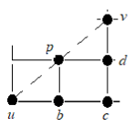
Figure 1: [3] $p\in\overline{uv}$ in a bounding curve, with $\overline{uv}$ slanted. Note $u\not\leftrightarrow_{c_{1}}p\not\leftrightarrow_{c_{1}}v$, $p\leftrightarrow_{c_{2}}c\not\leftrightarrow_{c_{1}}p$, $\{p,c\}\subset N(\mathbb{Z}^{2},c_{1},b)\cap N(\mathbb{Z}^{2},c_{1},d)$. If $X$ is thick then $c\in X$. (Not meant to be understood as showing all of $X$.)

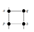
Figure 2: [3] $\angle apb$ is a $90^{\circ}$ ($\pi/2$ radians) angle of a bounding curve of $X$ at $p\in A_{1}$, with horizontal and vertical sides. If $X$ is thick then $q\in Int(X)$. (Not meant to be understood as showing all of $X$.)

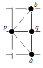
Figure 3: [3] $\angle apb$ is a $90^{\circ}$ ($\pi/2$ radians) angle between slanted segments of a bounding curve. If $X$ is thick then $q\in Int(X)$. (Not meant to be understood as showing all of $X$).

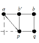
Figure 4: [3] $\angle apq$ is an angle of 135^∘ degrees ($3\pi/4$ radians) of a bounding curve of $X$ at $p$, with $\overline{ap}\cup\overline{pq}$ a subset of the bounding curve. If $X$ is thick then $b,b^{\prime}\in X$. (Not meant to be understood as showing all of $X$.)

2.4 Tools for determining fixed point sets

Material in this section is largely quoted or paraphrased from [3] and other references as indicated.

The following assertions are useful in determining fixed point and freezing sets.

Proposition 2.8.

(Corollary 8.4 of [4]) Let $(X,\kappa)$ be a digital image and $f\in C(X,\kappa)$. Suppose $x,x^{\prime}\in\operatorname{Fix}(f)$ are such that there is a unique shortest $\kappa$-path $P$ in $X$ from $x$ to $x^{\prime}$. Then $P\subset\operatorname{Fix}(f)$.

Lemma 2.9 below is in the spirit of “pulling” as introduced in [7]. We quote [2]:

The following assertion can be interpreted to say that in a $c_{u}$-adjacency, a continuous function that moves a point $p$ also [pulls along] a point that is “behind” $p$. E.g., in $\mathbb{Z}^{2}$, if $q$ and $q^{\prime}$ are $c_{1}$- or $c_{2}$-adjacent with $q$ left, right, above, or below $q^{\prime}$, and a continuous function $f$ moves $q$ to the left, right, higher, or lower, respectively, then $f$ also moves $q^{\prime}$ to the left, right, higher, or lower, respectively.

Lemma 2.9.

[2] Let $(X,c_{u})\subset\mathbb{Z}^{n}$ be a digital image, $1\leq u\leq n$. Let $q,q^{\prime}\in X$ be such that $q\leftrightarrow_{c_{u}}q^{\prime}$. Let $f\in C(X,c_{u})$.

1. If $p_{i}(f(q))>p_{i}(q)>p_{i}(q^{\prime})$ then $p_{i}(f(q^{\prime}))>p_{i}(q^{\prime})$.

2. If $p_{i}(f(q))<p_{i}(q)<p_{i}(q^{\prime})$ then $p_{i}(f(q^{\prime}))<p_{i}(q^{\prime})$.

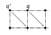
Figure 5: [3] Illustration of Lemma 2.9. Arrows show the images of $q,q^{\prime}$ under $f\in C(X,c_{2})$. Since $f(q)$ is to the right of $q$ and $q^{\prime}\leftrightarrow_{c_{1},c_{2}}q$ with $q^{\prime}$ to the left of $q$, $f$ pulls $q^{\prime}$ to the right so that $f(q^{\prime})$ is to the right of $q^{\prime}$.

Figure 5 illustrates Lemma 2.9.

Theorem 2.10.

[3] Let $D$ be a digital disk in $\mathbb{Z}^{2}$. Let $S$ be a bounding curve for $D$. Then $S$ is a freezing set for $(D,c_{1})$ and for $(D,c_{2})$.

Lemma 2.11.

Let $X\subset\mathbb{Z}^{2}$ and let $a,b\in X$ be such that $a$ and $b$ are endpoints of a slanted digital line segment $P\subset X$. Let $f\in C(X,c_{2})$ such that $\{a,b\}\subset\operatorname{Fix}(f)$. Then $P\subset\operatorname{Fix}(f)$.

Proof.

This assertion was proven in the proof of Theorem 4.2 of [3]. ∎

We will use the following.

Definition 2.12.

[3] Let $(X,\kappa)$ be a digital image. Let $p,q\in X$ such that

$$N(X,p,\kappa)\subset N^{*}(X,q,\kappa).$$

Then $q$ is a close $\kappa$-neighbor of $p$.

We say $X\subset\mathbb{Z}^{2}$ is

• symmetric with respect to the $x$-axis if $(x,y)\in X$ implies $(x,-y)\in X$;

• symmetric with respect to the $y$-axis if $(x,y)\in X$ implies $(-x,y)\in X$;

• symmetric with respect to the origin if $(x,y)\in X$ implies $(-x,-y)\in X$.

Proposition 2.13.

Let $X$ be a digital image.

• Suppose $X\subset\mathbb{Z}^{2}$ is symmetric with respect to the $x$-axis. If $p=(x,y)\in X$ has a close $c_{i}$-neighbor in $X$, then $p^{\prime}=(x,-y)$ has a close $c_{i}$-neighbor, $i\in\{1,2\}$.

• Suppose $X\subset\mathbb{Z}^{2}$ is symmetric with respect to the $y$-axis. If $p=(x,y)\in X$ has a close $c_{i}$-neighbor in $X$, then $p^{\prime}=(-x,y)$ has a close $c_{i}$-neighbor, $i\in\{1,2\}$.

• Suppose $X\subset\mathbb{Z}^{n}$ is symmetric with respect to the origin and $1\leq u\leq n$. If $p=(x,y)\in X$ has a close $c_{u}$ neighbor in $X$, then $p^{\prime}=(-x,-y)$ has a close $c_{u}$ neighbor in $X$.

Proof.

These assertions follow easily from Definition 2.12. ∎

Note these assertions are easily generalized to symmetry with respect to an arbitrary horizontal line, vertical line, or point, respectively.

Example 2.14.

A point $p$ with a close $\kappa$-neighbor $q$ need not be $\kappa$-adjacent to $q$. In the disk shown in Figure 7, $(1,1)$ is a close $c_{1}$-neighbor of $(0,0)$ but $(0,0)$ and $(1,1)$ are not $c_{1}$-adjacent. In the $c_{2}$-curve

$$X=\{(1,0),(0,1),(-1,0),(0,-1)\},$$

$(-1,0)$ is a close $c_{2}$-neighbor of $(1,0)$, but $(1,0)$ and $(-1,0)$ are not $c_{2}$-adjacent.

Lemma 2.15.

[4, 3] Let $(X,\kappa)$ be a digital image. Let $p,q\in X$ such that $q$ is a close $\kappa$-neighbor of $p$. Then $p$ belongs to every freezing set of $(X,\kappa)$.

However, in general a point of a freezing set for $(X,\kappa)$ need not have a close $\kappa$-neighbor in $X$, as shown by the following.

Example 2.16.

Let $X=[0,1]_{\mathbb{Z}}^{3}$. Let

$$A=\{(0,0,0),(0,1,1),(1,0,1),(1,1,0)\}.$$

See Figure 6. Then $A$ is a minimal freezing set for $(X,c_{1})$ [2]. However, it is easily seen that no member of $A$ has a close $c_{1}$-neighbor in $X$.

Figure 6: The unit 3-cube $X$, image of Example 2.16. Circled points make up a minimal $c_{1}$-freezing set, no member of which has a close $c_{1}$-neighbor in $X$.

3 $c_{1}$ results

In this section, we obtain results for freezing sets $(X,c_{1})$, with $X\subset\mathbb{Z}^{2}$.

Theorem 3.1.

[3] Let $X$ be a thick convex disk with a bounding curve $S$. Let $A_{1}$ be the set of points $x\in S$ such that $x$ is an endpoint of a maximal horizontal or a maximal vertical edge of $S$. Let $A_{2}$ be the union of slanted line segments in $S$. Then $A=A_{1}\cup A_{2}$ is a minimal freezing set for $(X,c_{1})$ (see Figure 7(ii)).

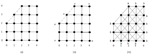
Figure 7: [3] The convex disk $D=[0,4]_{\mathbb{Z}}^{2}\setminus\{(0,3),(0,4),(1,4)\}$. The dashed segment from $(0,2)$ to $(2,4)$ shown in (i) and (ii) indicates part of a bounding curve and not $c_{1}$-adjacencies.
(i) $D$ with a $c_{2}$ bounding curve.
(ii) $(D,c_{1})$ with members of a minimal freezing set $A$ marked “a” - these are the endpoints of the maximal horizontal and vertical segments of the bounding curve, and all points of the slanted segment of the bounding curve, per Theorem 3.1.
(iii) $(D,c_{2})$ with members of a minimal freezing set $B$ marked “b” - these are the endpoints of the maximal slanted edge and all the points of the horizontal and vertical edges of the bounding curve, per Theorem 4.1.

Theorem 3.2.

Let $V_{i}\subset X\subset\mathbb{Z}^{2}$, $i\in\{1,\ldots,n\}$ where each $V_{i}$ is a thick convex disk. Let $X^{\prime}=\bigcup_{i=1}^{n}V_{i}$. Let $C_{i}$ be a bounding curve of $V_{i}$. Let $A_{1,i}$ be the set of endpoints of maximal horizontal or vertical segments of $C_{i}$. Let $A_{2,i}$ be the union of maximal slanted segments of $C_{i}$. Then $A=(X\setminus X^{\prime})\cup\bigcup_{i=1}^{n}(A_{1,i}\cup A_{2,i})$ is a freezing set for $(X,c_{1})$.

Proof.

Let $f\in C(X,c_{1})$ such that $A\subset\operatorname{Fix}(f)$. For each $i$, it follows from Proposition 2.8 that the horizontal and vertical segments whose endpoints are in $A_{1,i}$ belong to $\operatorname{Fix}(f)$; and it follows from our choice of $A_{2,i}$ that $C_{i}\subset\operatorname{Fix}(f)$. It follows from Proposition 2.8 that each horizontal segment joining two points of $C_{i}$ belongs to $\operatorname{Fix}(f)$. Since $V_{i}$ is convex, therefore $V_{i}\subset\operatorname{Fix}(f)$; hence $X^{\prime}\subset\operatorname{Fix}(f)$. Since by hypothesis, $X\setminus X^{\prime}\subset A\subset\operatorname{Fix}(f)$, we must have $Fix(f)=X$, and the assertion follows. ∎

In the following example, we show that the sets $\{V_{i}\}_{i=1}^{n}$ and $A$ of Theorem 3.2 are not in general unique, and $A$ may not be minimal.

Example 3.3.

Let $X=([0,2]_{\mathbb{Z}}\times[0,2]_{\mathbb{Z}})\cup([2,4]_{\mathbb{Z}}\times[0,3]_{\mathbb{Z}})$ (see Figure 8), for which the union above yields from Theorem 3.2 that

$$A=\{(0,0),(0,2),(2,0),(2,2),(2,3),(4,0),(4,3)\}$$

is a $c_{1}$-freezing set of $X$. Notice also that $X$ can be differently described as $X=([0,4]_{\mathbb{Z}}\times[0,2]_{\mathbb{Z}})\cup([2,4]_{\mathbb{Z}}\times[0,3]_{\mathbb{Z}})$ from which Theorem 3.2 yields a different freezing set,

$$F=\{(0,0),(0,2),(2,0),(2,3),(4,0),(4,2),(4,3)\}.$$

A minimal freezing set for $(X,c_{1})$ that is a proper subset of $A$ is

$$A^{\prime}=\{(0,0),(4,0),(4,3),(2,3),(0,2)\}.$$

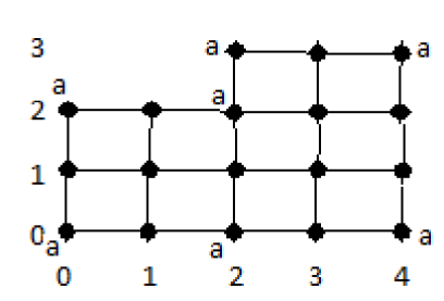
Figure 8: The digital image of Example 3.3. Points of the freezing set $A$ are marked “a”. For the minimal freezing set $A^{\prime}\subset A$, we have $\{(2,0),(2,2)\}\subset A\setminus A^{\prime}$.

Proof.

First, we show $A^{\prime}$ is a freezing set. Let $f\in C(X,c_{1})$ be such that $f|_{A^{\prime}}=\operatorname{id}_{A^{\prime}}$. From Proposition 2.8, the line segments

• from $(0,0)$ to $(0,2)$,

• from $(0,0)$ to $(4,0)$,

• from $(4,0)$ to $(4,3)$, and

• from $(4,3)$ to $(2,3)$

all belong to $\operatorname{Fix}(f)$. Therefore, by Proposition 2.8, the line segments

• from $(3,0)$ to $(3,3)$ and

• from $(2,0)$ to $(2,3)$

belong to $\operatorname{Fix}(f)$. Therefore, by Proposition 2.8, the line segment from $(0,2)$ to $(2,2)$ belongs to $\operatorname{Fix}(f)$. Therefore, by Proposition 2.8, the line segment from $(1,0)$ to $(1,2)$ belongs to $\operatorname{Fix}(f)$. Thus $X=\operatorname{Fix}(f)$, so $A^{\prime}$ is a freezing set for $(X,c_{1})$.

To show $A^{\prime}$ is minimal, observe that for every $p\in A^{\prime}$ there exists $q\in X$ such that $q$ is a close $c_{1}$-neighbor of $p$:

$(1,1)$ is a close $c_{1}$-neighbor of both $(0,0)$ and $(0,2)$:

$(3,1)$ is a close $c_{1}$-neighbor of $(4,0)$; and

$(3,2)$ is a close $c_{1}$-neighbor of both $(2,3)$ and $(4,3)$.

It follows from Lemma 2.15 that $p\in A^{\prime}$ implies $A^{\prime}\setminus\{p\}$ is not a freezing set for $(X,c_{1})$. The assertion follows. ∎

In light of Theorem 3.1, perhaps Theorem 3.2 will be especially useful for $c_{1}$-connected images that are not polygonal, as in the following.

Example 3.4.

Let $X$ be the union of the horizontal segments $[0,8]_{\mathbb{Z}}\times\{0\}$, $[0,3]\times\{1\}$, $[0,3]\times\{2\}$, $[6,8]_{\mathbb{Z}}\times\{1\}$, and $[7,8]_{\mathbb{Z}}\times\{2\}$ (see Figure 9). For the union $D_{1}\cup D_{2}$ of thick convex disks that are subsets of $X$, where

$$D_{1}=\{(x,y)\in X\,|\,x\leq 3\},~{}~{}~{}D_{2}=\{x,y)\in X\,|\,x\geq 6\},$$

with $D_{2}$ considered with a bounding curve including the segment from $(7,2)$ to $(6,1)$ (the dashed segment in Figure 9), Theorem 3.2 gives for $(X,c_{1})$ the freezing set

$$A=\left\{\begin{array}[]{l}(0,0),(0,2),(3,0),(3,2),(4,0),(5,0),\\ (6,0),(6,1),(7,2),(8,0),(8,2)\end{array}\right\}.$$ (2)

A minimal freezing set $A^{\prime}\subset A$ is

$$A^{\prime}=\{(0,0),(0,2),(3,2),(8,0),(8,2)\}.$$

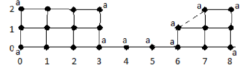
Figure 9: The digital image of Example 3.4. Points of the set $A$ of Theorem 3.2 are marked “a”, where $A$ is based on the union $D_{1}\cup D_{2}$ of thick convex disks that are subsets of $X$, where
$(x,y)\in D_{1}$ implies $x\leq 3$,
$(x,y)\in D_{2}$ implies $x\geq 6$, and
$D_{2}$ is considered with a bounding curve including the slanted segment from $(7,2)$ to $(6,1)$.

Proof.

Let $f\in C(X,c_{1})$ such that $A^{\prime}\subset\operatorname{Fix}(f)$. By (2) and Proposition 2.8, it follows that the horizontal segments $[0,8]_{\mathbb{Z}}\times\{0\}$ and $[0,3]_{\mathbb{Z}}\times\{2\}$ belong to $\operatorname{Fix}(f)$. It follows from Proposition 2.8 that the vertical segments $\{1\}\times[0,2]_{\mathbb{Z}}$ and $\{2\}\times[0,2]_{\mathbb{Z}}$ belong to $\operatorname{Fix}(f)$. By Proposition 2.8, the vertical segment from $(8,0)$ to $(8,2)$ belongs to $\operatorname{Fix}(f)$. This much shows $X\setminus\{(6,1),(7,1),(7,2)\}\subset\operatorname{Fix}(f)$.

Since $(6,1)\leftrightarrow_{c_{1}}(6,0)\in\operatorname{Fix}(f)$, we must have $p_{1}(f(6,1))\in\{5,6,7\}$.

• If $p_{1}(f(6,1))=5$ then by Lemma 2.9, $p_{1}(f(7,1))<7$ and $p_{1}(f(8,1))<8$, a contradiction since $(8,1)\in\operatorname{Fix}(f)$.

• If $p_{1}(f(6,1))=7$ then the continuity of $f$ requires that $(6,0)\not\in\operatorname{Fix}(f)$, a contradiction.

We conclude that $p_{1}(f(6,1))=6$.

Also since $(6,1)\leftrightarrow_{c_{1}}(6,0)\in\operatorname{Fix}(f)$, we must have, by continuity of $f$, $p_{2}(f(6,1))\in\{0,1\}$. If $p_{2}(f(6,1))=0$ then, since $f\in C(X,c_{1})$, either $p_{1}(f(7,1))=6$ or $p_{2}(f(7,1))=0$. In either case, the continuity of $f$ would require $(8,1)\not\in\operatorname{Fix}(f)$, a contradiction. Therefore, we must have $p_{2}(f(6,1))=1$, so $(6,1)\in\operatorname{Fix}(f)$.

Therefore, $(7,1)\in\operatorname{Fix}(f)$, by Proposition 2.8, since $(7,1)$ is on the unique shortest path between the fixed points $(6,1)$ and $(8,1)$.

Now we have $N(X,c_{1},(7,2))\subset\operatorname{Fix}(f)$, so the continuity of $f$ implies that $(7,2)\in\operatorname{Fix}(f)$.

Thus $X=\operatorname{Fix}(f)$, so $A^{\prime}$ is a freezing set.

To show $A^{\prime}$ is minimal, note that every $p\in A^{\prime}$ has a close $c_{1}$-neighbor in $X$:

$$\begin{array}[]{l}(1,1)\mbox{ is a close $c_{1}$-neighbor of both }(0,0)\mbox{ and }(0,2);\\ (2,1)\mbox{ is a close $c_{1}$-neighbor of }(3,2);\mbox{ and }\\ (7,1)\mbox{ is a close $c_{1}$-neighbor of both }(8,0)\mbox{ and }(8,2).\end{array}.$$

From Lemma 2.15 it follows that $A^{\prime}$ is a subset of every $c_{1}$-freezing set of $X$. The assertion follows. ∎

4 $c_{2}$ results

In this section, we derive a result for the $c_{2}$ adjacency that is dual to Theorem 3.2. We use the following.

Theorem 4.1.

[3] Let $X$ be a thick convex disk with a bounding curve $S$. Let $B_{1}$ be the set of points $x\in S$ such that $x$ is an endpoint of a maximal slanted edge in $S$. Let $B_{2}$ be the union of maximal horizontal and maximal vertical line segments in $S$. Let $B=B_{1}\cup B_{2}$. Then $B$ is a minimal freezing set for $(X,c_{2})$ (see Figure 7(iii)).

Theorem 4.2.

Let $V_{i}\subset X\subset\mathbb{Z}^{2}$, $i\in\{1,\ldots,n\}$ where each $V_{i}$ is a thick convex disk. Let $X^{\prime}=\bigcup_{i=1}^{n}V_{i}$. Let $C_{i}$ be a bounding curve of $V_{i}$. Let $B_{1,i}$ be the union of maximal horizontal and maximal vertical segments of $C_{i}$. Let $B_{2,i}$ be the set of endpoints of maximal slanted segments of $C_{i}$. Then $B=(X\setminus X^{\prime})\cup\bigcup_{i=1}^{n}(B_{1,i}\cup B_{2,i})$ is a freezing set for $(X,c_{1})$.

Proof.

Let $f\in C(X,c_{2})$ such that $B\subset\operatorname{Fix}(f)$. By hypothesis $B_{1,i}\subset\operatorname{Fix}(f)$. Let $S$ be a maximal slanted segment of $C_{i}$. Since $B_{2,i}\subset\operatorname{Fix}(f)$, Proposition 2.8 implies $S\subset\operatorname{Fix}(f)$. It follows that $C_{i}\subset\operatorname{Fix}(f)$. Since $V_{i}$ is convex, for every $x\in V_{i}$

• there is a vertical segment joining two members of $C_{i}$ and containing $x$; it follows from Lemma 2.9 that $p_{1}(f(x))=p_{1}(x)$; and

• there is a horizontal segment joining two members of $C_{i}$ and containing $x$; it follows from Lemma 2.9 that $p_{2}(f(x))=p_{2}(x)$. Hence $x\in\operatorname{Fix}(f)$.

Thus, for all $i$, $V_{i}\subset\operatorname{Fix}(f)$. Since by hypothesis, $X\setminus X^{\prime}\subset\operatorname{Fix}(f)$, it follows that $X=\operatorname{Fix}(f)$. Since $f$ is arbitrary, the assertion follows. ∎

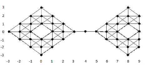
Figure 10: The digital image of Example 4.3. $X=\{(4,0)\}\cup\bigcup_{i=1}^{8}D_{i}$, where the $D_{i}$ are the thick convex disks listed below.
Subsets of $\{(x,y)\in X\,|\,x\leq 3\}$:
$~{}~{}~{}~{}~{}D_{1}$, with hull vertices $\{(-3,0),(0,3),(1,2),(-2,-1)\}$;
$~{}~{}~{}~{}~{}D_{2}$, with hull vertices $\{(1,2),(3,0),(2,-1),(0,1)\}$;
$~{}~{}~{}~{}~{}D_{3}$, with hull vertices $\{(2,-1),(0,-3),(-1,-2),(1,0)\}$; and
$~{}~{}~{}~{}~{}D_{4}$, with hull vertices $\{(-1,-2),(-2,-1),(-1,0),(0,-1)\}$.
Subsets of $\{(x,y)\in X\,|\,x\geq 5\}$:
$~{}~{}~{}~{}~{}D_{5}$, with hull vertices $\{(5,0),(7,2),(8,1),(6,-1)\}$,
$~{}~{}~{}~{}~{}D_{6}$, with hull vertices $\{(7,2),(8,3),(9,2),(9,0)\}$,
$~{}~{}~{}~{}~{}D_{7}$, with hull vertices $\{(9,0),(9,-2),(8,-3),(7,-2)\}$, and
$~{}~{}~{}~{}~{}D_{8}$, with hull vertices $\{(7,-2),(6,-1),(7,0),(8,-1)\}$.

Example 4.3.

Let $X\subset\mathbb{Z}^{2}$ be the digital image shown in Figure 10. The hull vertices listed for disks $D_{i}$ in this figure are all endpoints of maximal slanted bounding edges or members of horizontal or vertical bounding edges of their respective $D_{i}$. By Theorem 4.2, these hull vertices of the $D_{i}$; $(9,1)$ and $(9,-1)$, members of vertical bounding edges of $D_{6}$ and $D_{7}$, respectively; and $(4,0)\in X\setminus\bigcup_{i=1}^{8}D_{i}$, make up a freezing set $B$ for $(X,c_{2})$. Thus a listing of members of $B$ (note there are vertices that belong to more than one $D_{i}$):

$B=$

$$\left\{\begin{array}[]{l}(-3,0),(0,3),(1,2),(-2,-1),(3,0),(2,-1),(0,1),(0,-3),(-1,-2),\\ (1,0),(-1,0),(0,-1),(3,0),(4,0),(5,0),(7,2),(8,1),(6,-1),(8,3),(9,2),\\ (9,1),(9,0),(9,-1),(9,-2),(8,-3),(7,-2),(6,-1),(7,0),(8,-1)\end{array}\right\}$$

Let $B^{\prime}\subset B$ be the set

$$B^{\prime}=\{(-3,0),(0,-3),(0,3),(8,-3),(8,3),(9,-2),(9,-1),(9,1),(9,2)\}.$$

Then $B^{\prime}$ is a minimal freezing set for $(X,c_{2})$.

Proof.

Let $f\in C(X,c_{2})$ such that $B^{\prime}\subset\operatorname{Fix}(f)$. By Proposition 2.8, we have the following.

• The line segment $S_{1}$ from $(-3,0)$ to $(0,-3)$ belongs to $\operatorname{Fix}(f)$.

• The line segment $S_{2}$ from $(-3,0)$ to $(0,3)$ belongs to $\operatorname{Fix}(f)$.

• The path $S_{3}$ consisting of the line segment from $(0,-3)$ to $(3,0)$, the line segment from $(3,0)$ to $(5,0)$, and the line segment from $(5,0)$ to $(8,-3)$, belongs to $\operatorname{Fix}(f)$.

• The path $S_{4}$ consisting of the line segment from $(0,3)$ to $(3,0)$, the line segment from $(3,0)$ to $(5,0)$, and the line segment from $(5,0)$ to $(8,3)$, belongs to $\operatorname{Fix}(f)$.

• The line segment $S_{5}$ from $(8,-3)$ to $(9,-2)$ belongs to $\operatorname{Fix}(f)$.

• The line segment $S_{6}$ from $(8,3)$ to $(9,2)$ belongs to $\operatorname{Fix}(f)$.

Also, by hypothesis, the line segment $S_{7}$ from $(9,-1)$ to $(9,1)$ belongs to $\operatorname{Fix}(f)$. By the convexity of the $V_{i}$, every $x\in B^{\prime}\setminus\bigcup_{k=1}^{7}S_{k}$ belongs to a horizontal line segment between two members of $\bigcup_{k=1}^{7}S_{k}$; hence by Lemma 2.9, $p_{1}(f(x))=p_{1}(x)$. Also by the convexity of the $V_{i}$, every $x\in B^{\prime}\setminus\bigcup_{k=1}^{7}S_{k}$ belongs to a vertical line segment between two members of $\bigcup_{k=1}^{7}S_{k}$; hence by Lemma 2.9, $p_{2}(f(x))=p_{2}(x)$. Thus $x\in\operatorname{Fix}(f)$. Thus $X=\operatorname{Fix}(f)$, so $B^{\prime}$ is a freezing set.

Notice that every $p\in B^{\prime}$ has a close $c_{2}$-neighbor in $X$, as listed below.

$$\begin{array}[]{llc}p\in B^{\prime}&{}{}{}{}{}&\mbox{close }c_{2}\mbox{ neighbor of }p\mbox{ in }(X,c_{2})\\ (-3,0)&{}{}{}{}{}&(-2,0)\\ (0,-3)&{}{}{}{}{}&(0,-2)\\ (0,3)&{}{}{}{}{}&(0,2)\\ (8,-3)&{}{}{}{}{}&(8,-2)\\ (8,3)&{}{}{}{}{}&(8,2)\\ (9,-2)&{}{}{}{}{}&(8,-2)\\ (9,-1)&{}{}{}{}{}&(8,-1)\\ (9,1)&{}{}{}{}{}&(8,1)\\ (9,2)&{}{}{}{}{}&(8,2)\end{array}$$

By Lemma 2.15, $p$ belongs to every freezing set of $(X,c_{2})$. Therefore, $B^{\prime}$ is minimal. ∎

5 Further remarks

Theorems 3.2 and 4.2 give methods for finding a freezing set for $(X,c_{1})\subset\mathbb{Z}^{2}$ or $(X,c_{2})\subset\mathbb{Z}^{2}$, respectively. Roughly, a freezing set is found by filling $X$ as much as possible by thick convex disk subsets, then using the formula of the respective theorem. For both $c_{1}$ and $c_{2}$, the resulting freezing set can be examined, often using tools used in our examples, for a subset that is a minimal freezing set.

References

- [1] L. Boxer, A classical construction for the digital fundamental group, Journal of Mathematical Imaging and Vision 10 (1999), 51-62. https://link.springer.com/article/10.1023/A
- [2] L. Boxer, Fixed point sets in digital topology, 2, Applied General Topology 21(1) (2020), 111-133. https://polipapers.upv.es/index.php/AGT/article/view/12101
- [3] L. Boxer, Convexity and Freezing Sets in Digital Topology, submitted. Available at https://arxiv.org/abs/2005.09713
- [4] L. Boxer and P.C. Staecker, Fixed point sets in digital topology, 1, Applied General Topology 21 (1) (2020), 87-110. https://polipapers.upv.es/index.php/AGT/article/view/12091
- [5] L. Chen, Gradually varied surface and its optimal uniform approximation, SPIE Proceedings 2182 (1994), 300-307. https://www.spiedigitallibrary.org/conference-proceedings-of-spie/2182/0000/Gradually-varied-surface-and-its-optimal-uniform-approximation/10.1117/12.171078.short
- [6] L. Chen, Discrete Surfaces and Manifolds, Scientific Practical Computing, Rockville, MD, 2004. https://www.amazon.com/Discrete-Surfaces-Manifolds-Digital-Discrete-Geometry/dp/0975512218
- [7] J. Haarmann, M.P. Murphy, C.S. Peters, and P.C. Staecker, Homotopy equivalence in finite digital images, Journal of Mathematical Imaging and Vision 53 (2015), 288-302. https://link.springer.com/article/10.1007/s10851-015-0578-8
- [8] A. Rosenfeld, Digital topology, The American Mathematical Monthly 86 (8) (1979), 621-630. https://www.jstor.org/stable/2321290?seq=1
- [9] A. Rosenfeld, ‘Continuous’ functions on digital pictures, Pattern Recognition Letters 4, pp. 177-184, 1986. https://www.sciencedirect.com/science/article/pii/0167865586900176