Sobolev training of thermodynamic-informed neural networks for smoothed elasto-plasticity models with level set hardening

Abstract

We introduce a deep learning framework designed to train smoothed elastoplasticity models with interpretable components, such as a smoothed stored elastic energy function, a yield surface, and a plastic flow that are evolved based on a set of deep neural network predictions. By recasting the yield function as an evolving level set, we introduce a machine learning approach to predict the solutions of the Hamilton-Jacobi equation that governs the hardening mechanism. This machine learning hardening law may recover classical hardening models and discover new mechanisms that are otherwise very difficult to anticipate and hand-craft. This treatment enables us to use supervised machine learning to generate models that are thermodynamically consistent, interpretable, but also exhibit excellent learning capacity. Using a 3D FFT solver to create a polycrystal database, numerical experiments are conducted and the implementations of each component of the models are individually verified. Our numerical experiments reveal that this new approach provides more robust and accurate forward predictions of cyclic stress paths than these obtained from black-box deep neural network models such as a recurrent GRU neural network, a 1D convolutional neural network, and a multi-step feedforward model.

1 Introduction

Plastic deformation of materials is a history-dependent process manifested by irreversible and permanent changes of microstructures, such as dislocation, pore collapses, growth of defects and phase transition. Macroscopic consitutive models designed to capture the history-dependent constitutive responses can be categorized into multiple families. For example, hypoplasticity models often do not distinguish the reversible and irreversible strain (dafalias1986bounding; kolymbas1991outline; wang_identifying_2016). Unlike the classical elastoplasticity models where the plastic flow is normal to the stress gradient of the plastic potential and the evolution of it is governed by a set of hardening rules (rice1971inelastic; hill1998mathematical; sun_unified_2013; bryant2019micromorphically), hypoplasticity models do not employ a yield function to characterize the initial yielding. Instead, the relationship between the strain rate and the stress rate is captured by a set of evolution laws originated from a combination of phenomenological observations and physics constraints. Interestingly, the early design of neural network models such as ghaboussi_knowledge-based_1991; furukawa1998implicit; pernot1999application; lefik_artificial_2009, would often adopt this approach with a purely supervised learning strategy to adjust the weights of neurons to minimize the errors. Using the strain from current and previous time steps to estimate the current stress, these models would essentially predict the stress rate without utilizing a yield function and, hence, can be viewed as hypoplasticity models with machine learning derived evolution laws. The major issue of these machine learning generated evolution laws that, in retrospect, limits the adaptations of neural network constitutive model is the lack of interpretability and the vulnerability to over-fitting. While there are existing regularization techniques such as dropout layers (wang_multiscale_2018), cross-validation (heider2020so; vlassis2020geometric), adversarial attack (wang2020non) and/or increasing the size of the database could be helpful, it remains difficult to assess the credibility without the interpretability of the underlying laws deduced from the neural network. Another approach could involve symbolic regression through reinforcement learning (wang2019cooperative) or genetic algorithms (versino2017data) that may lead to explicitly written evolution laws, however, the fitness of these equations is often at the expense of readability.

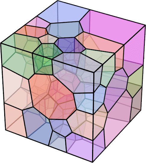
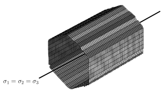
Figure 1: Neural network discovery of isotropic pressure-independent yield surface for polycrystal microstructure.

Another common approach to predict plastic deformation is the classical elasto-plasticity model where an elasticity model is coupled with a yield function that evolves with a set of internal variables that represents the history of the materials. Within the framework of the classical elasto-plasticity model – where constitutive models are driven by the evolution of yield surface and the underlying elastic model, there has been a significant number of works dedicated to refining the initial shapes and forms of the yield functions in the stress space (e.g. mises1913mechanik; prager1955theory; william1974constitutive) and the corresponding hardening laws that govern the evolution of these yield functions with the plastic strain (e.g. drucker1950some; borja1994multiaxial; taiebat2008sanisand; nielsen2010ductile; foster2005implicit; sun2014modeling). There are several key upshots brought by the existence of the yield function. For instance, the existence of a yield function facilitates the geometric interpretation of plasticity and, therefore, enables us to connect mechanics concepts, such as the thermodynamic law, with geometric concepts, such as convexity in the principal stress space (miehe_anisotropic_2002; borja_plasticity_2013; vlassis2020geometric). Furthermore, the existence of a distinctive elastic region in the stress or strain space also allows to introduce a multi-step transfer learning strategy. In this case, the machine learning of the elastic responses can be viewed as a pre-training step for the plasticity machine learning where the predicted elastic responses can help determine the underlying split of the elastic and plastic strain upon the initial yielding and, hence, allows for a more accurate hardening law and plastic flow to be discovered.

1.1 Why Sobolev training for plasticity

Recently, there have been attempts to rectify the limitations of machine learning models that do not distinguish or partition the elastic and plastic strain. xu2020learning, for instance, introduce a differentiable transition function to create a smooth transition between the elastic and plastic range for an incremental constitutive law generated from supervised learning. mozaffar2019deep and later zhang2020using inroduce the machine learning to deduce the yield function and enable linear and distortion hardening using loss functions that minimizing the $L_{2}$ norm of the yield function discrepancy.

While these machine learning exercises are effective in identifying the yield locus, calibrating and even selecting the existing hardening mechanisms ((isotropic, kinematic, rotation….etc)) for predictions, more flexibility and control over capturing the evolution of the yield surface with respect to strain history is needed for more general applications where the dominated hardening mechanisms are not known in advance. Furthermore, since the constitutive laws are updated via a system of linearized constrains, the solvability of the constitutive laws and the resultant global system of equations all depends not only on the accuracy of the predictions of the yield function, but also the gradient and Hessian.

This research is specifically designed to fill this knowledge gap in order to make the machine learning models more robust and practical when incorporating into PDE solvers. In particular, we introduce a set of new supervised learning problems where a family of higher-order norms is used to regularize the predictions of scalar functionals that lead to the elastic and elasto-plastic responses of isotropic path-dependent materials. By adopting the Haigh-Westergaard coordinate system to simplify the parametrization, we introduce a simple training program that can generate accurate and robust stress predictions but also yield the elastic energy and elasto-plastic tangent operator that is sufficiently smooth for numerical predictions – one of the technical barriers that prevent the adoption of neural network models since their inception in the 90s (hashash2004numerical).

1.2 Organization of the content and notations

The organization of the rest of the paper is as follows. We first provide a detailed account of the different designs of Sobolev higher-order training introduced to generate the elastic stored energy functional, yield function, flow rules and hardening models in their corresponding parametric space. The setup of control experiments with other common alternative black-box models is then described. We then demonstrate how to leverage this new design of an interpretable machine learning framework to analyze the thermodynamic behavior of the machine learning derived constitutive laws, while illustrating the geometrical interpretation of the proposed modeling framework. A brief highlight for the adopted return mapping algorithm implementation that leverages automatic differentiation is provided in Section LABEL:sec:return_mapping_algorithm, followed by the numerical experiments and the conclusions that outline this work’s major findings.

As for notations and symbols in this current work, bold-faced letters denote tensors (including vectors which are rank-one tensors); the symbol ’$\cdot$’ denotes a single contraction of adjacent indices of two tensors (e.g. $\boldsymbol{a}\cdot\boldsymbol{b}=a_{i}b_{i}$ or $\boldsymbol{c}\cdot\boldsymbol{d}=c_{ij}d_{jk}$ ); the symbol ‘:’ denotes a double contraction of adjacent indices of tensor of rank two or higher ( e.g. $\boldsymbol{C}:\boldsymbol{\epsilon^{e}}$ = $C_{ijkl}\epsilon_{kl}^{e}$ ); the symbol ‘$\otimes$’ denotes a juxtaposition of two vectors (e.g. $\boldsymbol{a}\otimes\boldsymbol{b}=a_{i}b_{j}$) or two symmetric second order tensors (e.g. $(\boldsymbol{\alpha}\otimes\boldsymbol{\beta})_{ijkl}=\alpha_{ij}\beta_{kl}$). Moreover, $(\boldsymbol{\alpha}\oplus\boldsymbol{\beta})_{ijkl}=\alpha_{jl}\beta_{ik}$ and $(\boldsymbol{\alpha}\ominus\boldsymbol{\beta})_{ijkl}=\alpha_{il}\beta_{jk}$. We also define identity tensors $(\boldsymbol{I})_{ij}=\delta_{ij}$, $(\boldsymbol{I}^{4})_{ijkl}=\delta_{ik}\delta_{jl}$, and $(\boldsymbol{I}^{4}_{\text{sym}})_{ijkl}=\frac{1}{2}(\delta_{ik}\delta_{jl}+\delta_{il}\delta_{kj})$, where $\delta_{ij}$ is the Kronecker delta. As for sign conventions, unless specified otherwise, we consider the direction of the tensile stress and dilative pressure as positive.

2 Framework for Sobolev training of elastoplasticity models

This section presents the framework to train the multiple deep neural networks to predict the three constitutive laws studied in this work – the elastic stored energy functional, the yield function, and the plastic flow.

We discuss the neural network architecture that will allow for smoother predictions and higher-order Sobolev optimization. We introduce how this higher-order training can benefit the data-driven approximation of a hyperelastic energy functional. Continuing with plasticity, we describe how we achieve the dimensionality reduction of our training problem by adopting the $\pi$-plane interpretation of the stress space. The yield function prediction and evolution is presented as a Hamilton-Jacobi extension problem to facilitate the data pre-processing and neural network training. Finally, the training objectives for associative and non-associative plasticity laws that obey thermodynamic constraints are described.

To simplify the proposed constitutive laws, we assume that the deformation is infinitesimal and the plastic deformation is rate independent. Meanwhile, the elastic response and the initial yield function of the materials we considered can both be approximated as isotropic. Extensions that relax these assumptions will be considered in future studies but is out of the scope of this current paper.

2.1 Neural network design for Sobolev training of a smooth scalar functional with physical constraints

Here we will provide a brief account on the design of the neural network that aims to generate a scalar functional with sufficient smoothness and continuity for a variety of mechanics problems where both the functional itself and its derivatives are both of interest (e.g. elasticity energy functional, yield function). The specific data preparation and the loss function required to complete the Sobolev training will be discussed in the next Sections 2.2 and 2.3.

Architecture: ddd	Architecture: dmdd	Architecture: dmdmd	Architecture: dmmdmd

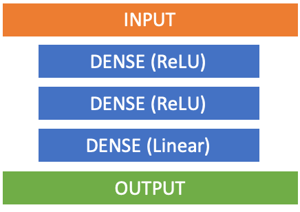
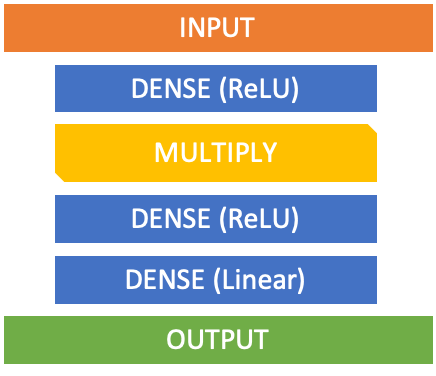
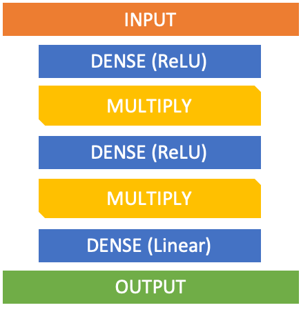
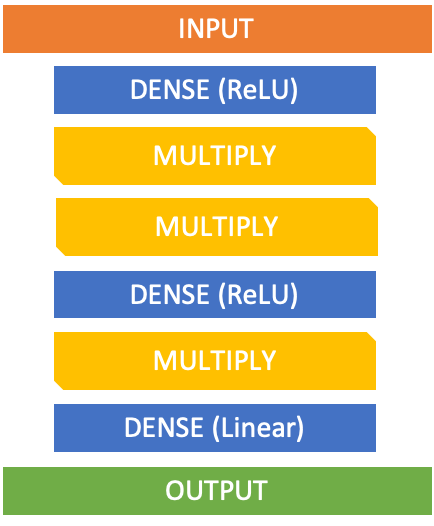
Figure 2: Modification of standard two-layer feed-forward architecture with the introduction of Multiply layers that increase local non-linearity. For brevity, the letters d and m represent the Dense and Multiply layers respectively that form an architecture (e.g. architecture dmdd has the layer structure Dense $\rightarrow$ Multiply $\rightarrow$ Dense $\rightarrow$ Dense).

While many common tasks that employ supervised learning such as classification of images and game playing, rarely mandate accurate predictions of the approximated function’s derivatives, while computational mechanics problems that are based on variational principle often require their determination.

To facilitate the Sobolev training, we must employ a setup to ensure that the learned function is an element of a Sobolev space. First, we must define the norm and loss function to measure the distance between the approximated function and the benchmark. Second, we must introduce the types of activities such that the basis of the learned function spans a Sobolev space. Most feed-forward neural network architectures used for regression utilize a combination of linear or piece-wise linear activation functions. For example, a common architecture for regression may employ the ReLU activation function, $\text{ReLU}(\bullet)=\max(0,\bullet)$, for the intermediate hidden layers of the network and the linear activation function, $\text{Linear}(\bullet)=\bullet$, for the output layer. The second-order derivative of such architecture with respect to the input would be constant and equal to zero and, hence, not suitable for our purpose where the second derivatives of the potentials are essential.

To ensure the degree of continuity of the learned function to gain control of the errors of the higher-order derivatives, we introduce a simple technique of adding Multiply layers. These layers are placed in between two hidden dense layers of the network to modify the output of the preceding layer. The Multiply layer receives as input the output $\boldsymbol{h}^{n-1}$ of the preceding layer and outputs $\boldsymbol{h}^{n}$, such that,

$$\boldsymbol{h}^{n}=\text{Multiply}(\boldsymbol{h}^{n-1})=\boldsymbol{h}^{n-1}\circ\boldsymbol{h}^{n-1},$$ (1)

where $\circ$ is the element-wise product of two-vectors. Conceptually, introducing a Multiply layer is equivalent to modifying the activation function of the preceding layer. By placing the Multiply layers in between dense layers, this simple modification enables us to control the order of continuity of the learned multivariable function. Without the introduction of any additional weights or handcrafting custom activation functions, this simple technique provides a simple solution to overcome the issue of vanishing 2nd-order derivatives that would impede the training and the deployment of machine learning elastoplasticity models that heavily rely on the network’s differentiability.

The placement and the number of intermediate Multiply layers are hyper-parameters that can be fine-tuned along with the rest of the hyperparameters of the neural network (e.g. dropout rate, number of neurons per layer, number of layers). The tuning of these hyperparameters can be performed manually or through automatic hyperparameter tuning algorithms (cf. bergstra2015hyperopt; komer2014hyperopt). Several variations to the standard two-layer architecture we tested for shown in Fig. 2. The performance of these different neural networks that complete the higher-order Sobolev training is demonstrated in the numerical experiments showcased in Section LABEL:sec:small_strain_sobolev.

2.2 Sobolev training of hyperelastic energy functional

The first component of the elastoplastic framework we train is the elastic stored energy $\psi^{e}$. The elasticity energy functional is not only useful for predicting the stress from the elastic strain, but can also be used to re-interpret the experimental data to identify the accumulated plastic strain and the plastic flow directions that are crucial for the training of the yield function and plastic flow.

In the infinitesimal strain regime, the hyperelastic energy functional $\psi^{\mathrm{e}}(\boldsymbol{\epsilon}^{\mathrm{e}})\in\mathbb{R}^{+}$ can be define as a non-negative valued function of elastic infinitesimal strain of which the first derivative is the Cauchy stress tensor $\boldsymbol{\sigma}\in\mathbb{S}$ and the Hessian is the tangential elasticity tensor $\boldsymbol{c}^{e}\in\mathbb{M}$:

$$\boldsymbol{\sigma}=\frac{\partial\psi^{\mathrm{e}}\left(\boldsymbol{\epsilon}^{\mathrm{e}}\right)}{\partial\boldsymbol{\epsilon}^{\mathrm{e}}}\;,\;\boldsymbol{c}^{\mathrm{e}}=\frac{\partial\boldsymbol{\sigma}}{\partial\boldsymbol{\epsilon}^{\mathrm{e}}}=\frac{\partial^{2}\psi^{\mathrm{e}}\left(\boldsymbol{\epsilon}^{\mathrm{e}}\right)}{\partial\boldsymbol{\epsilon}^{\mathrm{e}}\otimes\partial\boldsymbol{\epsilon}^{\mathrm{e}}},$$ (2)

where $\mathbb{S}$ is the space of the second-order symmetric tensors and $\mathbb{M}$ is the space of the fourth-order tensors that possess major and minor symmetries (heider2020so). The true hyperelastic energy functional $\psi^{\mathrm{e}}$ of the material is approximated by the neural network learned function $\widehat{\psi}^{\mathrm{e}}(\boldsymbol{\epsilon}^{\mathrm{e}}|\boldsymbol{W},\boldsymbol{b})$ with the elastic strain tensor $\boldsymbol{\epsilon}^{\mathrm{e}}$ as the input, parametrized by weights $\boldsymbol{W}$ and biases $\boldsymbol{b}$ obtained from a supervised learning procedure.

In a conventional setting, the training often employs the mean square error or the $L_{2}$ norm as the loss function. The $L_{2}$ norm training objective for the training samples $i\in[1,...,N]$ takes the following form:

$$\boldsymbol{W}^{\prime},\boldsymbol{b}^{\prime}=\operatorname*{argmin}_{\boldsymbol{W},\boldsymbol{b}}\left(\frac{1}{N}\sum_{i=1}^{N}\gamma_{1}\left\lVert\psi^{\mathrm{e}}-\widehat{\psi}^{\mathrm{e}}_{i}\right\rVert^{2}_{2}\right),$$ (3)

where $\gamma_{1}$ is a scaling coefficient discussed further in Remark 1.

However, the issue is that the convergence of the stored energy measured by the $L_{2}$ norm does not guarantee the quality and even the existence of the stress and elastic tangent operators stemmed from the learned energy function. To rectify this issue, we introduce the use of an $H^{1}$ norm as the loss function to train a generic anisotropic energy functional that predict the polycrystal elasticity in finite deformation regime vlassis2020geometric. In the infinitesimal regime, the supervised learning procedure is to find the weights and biases for the neural network such that,

$$W^{\prime},\boldsymbol{b}^{\prime}=\underset{\boldsymbol{W},\boldsymbol{b}}{\operatorname{argmin}}\left(\frac{1}{N}\sum_{i=1}^{N}\left(\gamma_{1}\left\|\psi^{\mathrm{e}}_{i}-\widehat{\psi}^{\mathrm{e}}_{i}\right\|_{2}^{2}+\gamma_{2}\left\|\frac{\partial\psi^{\mathrm{e}}_{i}}{\partial\boldsymbol{\epsilon}^{\mathrm{e}}_{i}}-\frac{\partial\widehat{\psi}^{\mathrm{e}}_{i}}{\partial\boldsymbol{\epsilon}^{\mathrm{e}}_{i}}\right\|_{2}^{2}\right)\right),$$ (4)

where we assume that both the energy and the stress measures are sampled together at each data point and the total number of sample is $N$. In this work, our goal is to generate elasto-plastic model that is practical for implicit solvers. This, however, is considered a difficult task in the earlier attempts on using neural network as a replacement for constitutive laws (cf. hashash2004numerical) and, hence, the proposed solution is either to bypass the calculation of tangent with an explicit time integrator or to introduce finite differences on the stress predictions.

By leveraging the differentiability achieved by the Multiply layer and adopting an $H^{2}$ norm as the training objective, we introduce an alternative that renders the neural network model applicable for implicit solver while eliminating the potential spurious oscillations of the tangent operators. The new training objective for the hyperelastic energy functional approximator $\widehat{\psi}^{\mathrm{e}}$ includes constraints for the predicted energy, stress, and stiffness values. This training objective, modeled after an $H^{2}$ norm, for the training samples $i\in[1,...,N]$ would have the following form:

$$W^{\prime},\boldsymbol{b}^{\prime}=\underset{\boldsymbol{W},\boldsymbol{b}}{\operatorname{argmin}}\left(\frac{1}{N}\sum_{i=1}^{N}\left(\gamma_{1}\left\|\psi^{\mathrm{e}}_{i}-\widehat{\psi}^{\mathrm{e}}_{i}\right\|_{2}^{2}+\gamma_{2}\left\|\frac{\partial\psi^{\mathrm{e}}_{i}}{\partial\boldsymbol{\epsilon}^{\mathrm{e}}_{i}}-\frac{\partial\widehat{\psi}^{\mathrm{e}}_{i}}{\partial\boldsymbol{\epsilon}^{\mathrm{e}}_{i}}\right\|_{2}^{2}+\gamma_{3}\left\|\frac{\partial^{2}\psi^{\mathrm{e}}_{i}}{\partial\boldsymbol{\epsilon}^{\mathrm{e}}_{i}\otimes\partial\boldsymbol{\epsilon}^{\mathrm{e}}_{i}}-\frac{\partial^{2}\widehat{\psi}^{\mathrm{e}}_{i}}{\partial\boldsymbol{\epsilon}^{\mathrm{e}}_{i}\otimes\partial\boldsymbol{\epsilon}^{\mathrm{e}}_{i}}\right\|_{2}^{2}\right)\right).$$ (5)

2.2.1 Simplified training for isotropic elasticity

In this work, our primary focus is on small strain isotropic hyperelasticity which can completely be described in spectral form by the principal strain and stress values (without the principal directions). Thus, for isotropic infinitesimal hyperelasticity, the $H_{2}$ training objective of Eq. (5) for the training samples $i\in[1,...,N]$ can be rewritten in terms of principal values as:

$$W^{\prime},\boldsymbol{b}^{\prime}=\underset{\boldsymbol{W},\boldsymbol{b}}{\operatorname{argmin}}\Bigl{(}\frac{1}{N}\sum_{i=1}^{N}\Bigl{(}\gamma_{1}\left\|\psi^{\mathrm{e}}_{i}-\widehat{\psi}^{\mathrm{e}}_{i}\right\|_{2}^{2}+\sum_{A=1}^{3}\gamma_{2}\left\|\frac{\partial\psi^{\mathrm{e}}_{i}}{\partial\epsilon^{\mathrm{e}}_{A,i}}-\frac{\partial\widehat{\psi}^{\mathrm{e}}_{i}}{\partial\epsilon^{\mathrm{e}}_{A,i}}\right\|_{2}^{2}$$

$$+\sum_{A=1}^{3}\sum_{B=1}^{3}\gamma_{3}\left\|\frac{\partial^{2}\psi^{\mathrm{e}}_{i}}{\partial\epsilon^{\mathrm{e}}_{A,i}\partial\epsilon^{\mathrm{e}}_{B,i}}-\frac{\partial^{2}\widehat{\psi}^{\mathrm{e}}_{i}}{\partial\epsilon^{\mathrm{e}}_{A,i}\partial\epsilon^{\mathrm{e}}_{B,i}}\right\|_{2}^{2}\Bigr{)}\Bigr{)},$$ (6)

where $\epsilon^{\mathrm{e}}_{A}$ for $A=1,2,3$ are the principal values of the elastic strain tensor $\boldsymbol{\epsilon}^{\mathrm{e}}$. The approximated energy functional for this training objective is a function of the three input principal strains and not of a full second-order tensor of 6 input components (reduced from 9 by assuming symmetry). This effectively reduces the input parametric space of the learned function and facilitates learning by minimizing complexity.

The training objective can further be simplified to two input variables by adopting an invariant space, commonly used in geotechnical studies when the intermediate principal stress does not exhibit a dominating effect on the elastic response or when the intermediate principal stress is not measured at all due to the limitation of the experiment apparatus (wawersik1997new; haimson2010effect). In this case, a small-strain isotropic hyperelastic law can equivalently be described with two strain invariants (volumetric strain $\epsilon_{v}^{\mathrm{e}}$, deviatoric strain $\epsilon_{s}^{\mathrm{e}}$). The strain invariants are defined as:

$$\epsilon_{v}^{\mathrm{e}}=\operatorname{tr}\left(\boldsymbol{\epsilon}^{\mathrm{e}}\right),\quad\epsilon_{s}^{\mathrm{e}}=\sqrt{\frac{2}{3}}\left\|\boldsymbol{e}^{\mathrm{e}}\right\|,\quad\boldsymbol{e}^{\mathrm{e}}=\boldsymbol{\epsilon}^{\mathrm{e}}-\frac{1}{3}\epsilon_{v}^{\mathrm{e}}\boldsymbol{1},$$ (7)

where $\boldsymbol{\epsilon}^{\mathrm{e}}$ is the small strain tensor and $\boldsymbol{e}^{\mathrm{e}}$ the deviatoric part of the small strain tensor. Using the chain rule, the Cauchy stress tensor can be described in the invariant space as follows:

$$\boldsymbol{\sigma}=\frac{\partial\psi^{\mathrm{e}}}{\partial\epsilon_{v}^{\mathrm{e}}}\frac{\partial\epsilon_{v}^{\mathrm{e}}}{\partial\boldsymbol{\epsilon}^{\mathrm{e}}}+\frac{\partial\psi^{\mathrm{e}}}{\partial\epsilon_{s}^{\mathrm{e}}}\frac{\partial\epsilon_{s}^{\mathrm{e}}}{\partial\boldsymbol{\epsilon}^{\mathrm{e}}}.$$ (8)

In the above, the mean pressure $p$ and deviatoric (von Mises) stress $q$ can be defined as:

$$p=\frac{\partial\psi^{\mathrm{e}}}{\partial\epsilon_{v}^{\mathrm{e}}}\equiv\frac{1}{3}\operatorname{tr}(\boldsymbol{\sigma}),\quad q=\frac{\partial\psi^{\mathrm{e}}}{\partial\epsilon_{s}^{\mathrm{e}}}\equiv\sqrt{\frac{3}{2}}\|\boldsymbol{s}\|,$$ (9)

where $\boldsymbol{s}$ is the deviatoric part of the Cauchy stress tensor. Thus, the Cauchy stress tensor can be expressed by the stress invariants as:

$$\boldsymbol{\sigma}=p\mathbf{1}+\sqrt{\frac{2}{3}}q\widehat{\boldsymbol{n}},$$ (10)

$$\text{where}\>\>\widehat{\boldsymbol{n}}=\boldsymbol{e}^{\mathrm{e}}/\left\|\boldsymbol{e}^{\mathrm{e}}\right\|=\sqrt{2/3}e^{\mathrm{e}}/\epsilon_{s}^{\mathrm{e}}.$$ (11)

The $H_{2}$ training objective of Eq. (6) for the training samples $i\in[1,...,N]$ can now be rewritten in terms of the two strain invariants:

$$\boldsymbol{W}^{\prime},\boldsymbol{b}^{\prime}=\underset{\boldsymbol{W},\boldsymbol{b}}{\operatorname{argmin}}\Bigl{(}\frac{1}{N}\sum_{i=1}^{N}\Bigl{(}\gamma_{1}\left\|\psi^{\mathrm{e}}_{i}-\widehat{\psi}^{\mathrm{e}}_{i}\right\|_{2}^{2}+\gamma_{4}\left\|p_{i}-\widehat{p}_{i}\right\|_{2}^{2}$$

$$+\gamma_{5}\left\|q_{i}-\widehat{q}_{i}\right\|_{2}^{2}+\sum_{\alpha=1}^{2}\sum_{\beta=1}^{2}\gamma_{6}\left\|D_{\alpha\beta,i}^{\mathrm{e}}-\widehat{D}_{\alpha\beta,i}^{\mathrm{e}}\right\|_{2}^{2}\Bigr{)}\Bigr{)},$$ (12)

where:

$$D_{11}^{\mathrm{e}}=\frac{\partial^{2}\psi}{\partial\epsilon_{v}^{\mathrm{e}\,2}},\quad D_{22}^{\mathrm{e}}=\frac{\partial^{2}\psi}{\partial\epsilon_{s}^{\mathrm{e}\,2}},\quad\text{and}\quad D_{12}^{\mathrm{e}}=D_{21}^{\mathrm{e}}=\frac{\partial^{2}\psi}{\partial\epsilon_{v}^{\mathrm{e}}\partial\epsilon_{s}^{\mathrm{e}}}.$$ (13)

Finally, it should be noted that while the loss function listed in Eqs. (6) and (12) is sufficient to control all degree of freedoms for the stored energy, the stress and the tangent simultaneously for the isotropic and two-invariant cases, these two loss functions can also be used for the general anisotropic case if only partial control on the stress and tangent is needed.

Remark 1.

Rescaling of the training data. The terms of the loss functions mentioned in this section constrain measures of different units (energy, stress, stiffness). In every loss function in this work, we have introduced scaling coefficients $\gamma_{\alpha}$ for consistency of the units in the formulation. In practice, as pre-processing step all input and output measures used in neural network training have been scaled to a unitless feature range from 0 to 1. Thus, the use of other scaling unit coefficients was not deemed necessary during training.

2.3 Training of evolving yield function as level set

This section introduces the theoretical framework that regards the evolution of the yield surface as a level set evolution problem. To illustrate the key ideas with a visual geometrical interpretation and without the burden of generating a large database, we restrict our attentions to construct a yield function that remains pressure-insensitive (Fig. 1) but may otherwise evolve in any arbitrary way on the $pi$-plane, including moving, expanding, contracting and deforming the elastic region. The goal of the supervised learning task is to determine the optimal way the yield function should evolve such that it is consistent with the observed experimental data collected after the plastic yielding and obeying the thermodynamic constraints that can be interpreted geometrically in the stress space.

2.3.1 Reducing the dimension of data by leveraging symmetries

Here we provide a brief review of the geometrical interpretation of the stress space and how it can be used to reduce the dimensions of the data and reduce the difficulty of the machine learning tasks. In this work, we consider a convex elastic domain $\mathbb{E}$ defined by a yield surface $f$. This yield function is a function of Cauchy stress $\boldsymbol{\sigma}$ and the internal variable $\xi$ that represent the history-dependent behavior of the material, i.e., (cf. borja_plasticity_2013),

$$\xi=\int_{0}^{t}\dot{\lambda}dt,$$ (14)

where $\xi$ is an monotonically increasing function of time and $\dot{\lambda}$ is the rate of change of the plastic multiplier where $\dot{\boldsymbol{\epsilon}}^{p}=\dot{\lambda}\partial g/\partial\boldsymbol{\sigma}$ and $g$ is the plastic potential. The yield function returns a negative value in the elastic region and equals to zero when the material is yielding. The stress on the boundary $f(\boldsymbol{\sigma},\xi)=0$ is therefore the yielding stress and all admissible stress belong to the closure of the elastic domain, i.e.,

$$\mathbb{E}:=\{(\boldsymbol{\sigma},\xi)\in\mathbb{S}\times\mathbb{R}^{1}|f(\boldsymbol{\sigma},\xi)\leq 0\}.$$ (15)

First, we assume that the yield function depends only on the principal stress. This treatment reduces the dimension of the stress from six to three. Then, we assume that the plastic yielding is not sensitive to the mean pressure. As such, the shape of the yield surface in the principal stress space can be sufficiently described by a projection on the $\pi$-plane and, hence, further reduce the dimensions of the independent stress input from three to two. To further simplify the interpolation of the yield surface, we introduce a polar coordinate system on the $\pi$-plane such that different monotonic stress paths commonly obtained from triaxial tests can be easily described via the Lode’s angle.

Recall that the $\pi$-plane refers to a projection of the principal stress space based on the space diagonal defined by $\sigma_{1}=\sigma_{2}=\sigma_{3}$. More specifically, the $\pi$-plane is defined by the equation:

$$\sigma_{1}+\sigma_{2}+\sigma_{3}=0.$$ (16)

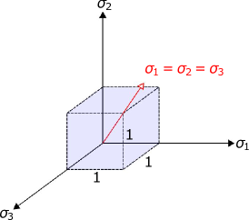
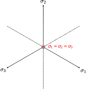
Figure 3: The $\pi$-plane is perpendicular to the space diagonal and is passing through the origin of the principal stress axes. Figure reproduced from borja_plasticity_2013.

The transformation from the original stress space coordinate system $(\sigma_{1},\sigma_{2},\sigma_{3})$ to the $\pi$-plane can be decomposed into two specific rotations $\boldsymbol{R}$ and $\boldsymbol{R^{\prime\prime}}$ of the coordinate system (cf. (borja_plasticity_2013)) such that,

$$\left\{\begin{array}[]{l}\sigma_{1}\\ \sigma_{2}\\ \sigma_{3}\end{array}\right\}=\boldsymbol{R}^{\prime}\boldsymbol{R}^{\prime\prime}\left\{\begin{array}[]{c}\sigma_{1}^{\prime\prime}\\ \sigma_{2}^{\prime\prime}\\ \sigma_{3}^{\prime\prime}\end{array}\right\}=\left[\begin{array}[]{ccc}\sqrt{2}/2&0&\sqrt{2}/2\\ 0&1&0\\ -\sqrt{2}/2&0&\sqrt{2}/2\end{array}\right]\left[\begin{array}[]{ccc}1&0&0\\ 0&\sqrt{2/3}&1/\sqrt{3}\\ 0&-1/\sqrt{3}&\sqrt{2/3}\end{array}\right]\left\{\begin{array}[]{c}\sigma_{1}^{\prime\prime}\\ \sigma_{2}^{\prime\prime}\\ \sigma_{3}^{\prime\prime}\end{array}\right\}$$ (17)

For pressure-insensitive plasticity, $\sigma_{3}^{\prime\prime}$ is not needed, as the principal stress differences are function of $\sigma_{1}^{\prime\prime}$ and $\sigma_{2}^{\prime\prime}$ and are independent of $\sigma_{3}^{\prime\prime}$.

We opt to describe the stress states of the material on the $\pi$-plane using two stress invariants, the polar radius $r$ and the Lode’s angle $\theta$ (lode1926versuche). These invariants are derived by solving the characteristic equation of the deviatoric component $\boldsymbol{s}\in\mathbb{S}$ of the Cauchy stress tensor, following (borja_plasticity_2013):

$$s^{3}-J_{2}s-J_{3}=0,$$ (18)

where $s$ is a principal value of $\boldsymbol{s}$, and

$$J_{2}=\frac{1}{2}\text{tr}(\boldsymbol{s}^{2}),\qquad J_{3}=\frac{1}{3}\text{tr}(\boldsymbol{s}^{3}),$$ (19)

are respectively the second and third invariants of the tensor $\boldsymbol{s}$. Utilizing the identity:

$$\cos^{3}\theta-3/4\cos\theta-1/4\cos 3\theta=0,$$ (20)

and writing $s$ in polar coordinates such that:

$$s=\rho\cos\theta,$$ (21)

and substituting in (18), the polar radius and the Lode’s angle, can be retrieved as:

$$\rho=2\sqrt{J_{2}/3},\qquad\text{and}\qquad\cos 3\theta=\frac{3\sqrt{3}J_{3}}{2J_{2}^{3/2}}.$$ (22)

In terms of the $\pi$-plane coordinates $\sigma_{1}^{\prime\prime}$ and $\sigma_{2}^{\prime\prime}$, the Lode’s coordinates $\rho$ and $\theta$ can be respectively written as:

$$\rho=\sqrt{\sigma_{1}^{\prime\prime\,2}+\sigma_{2}^{\prime\prime\,2}},\qquad\text{and}\qquad\tan\theta=\frac{\sigma_{2}^{\prime\prime}}{\sigma_{1}^{\prime\prime}}.$$ (23)

Thus, for an isotropic pressure-independent plasticity model, the yield surface can equivalently be described by an approximator using either the principal stresses $\sigma_{1}$, $\sigma_{2}$, and $\sigma_{3}$ or the stress invariant $\rho$, and, $\theta$ such that:

$$\overline{f}(\sigma_{1},\sigma_{2},\sigma_{3},\xi)=\widehat{f}(\rho,\theta,\xi)=0.$$ (24)

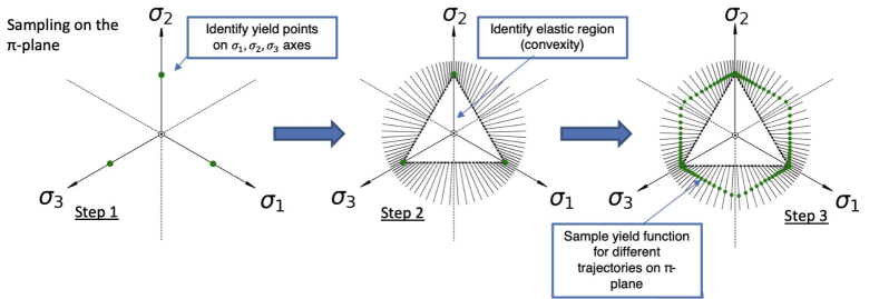
Figure 4: The $\pi$-plane is used as the basis for the polycrystal plasticty dataset generation. The plane is explored radially for different Lode angle inputs. Every Lode angle constitutes a different simulation. The material is first loaded in the direction of $\sigma_{1}$, $\sigma_{2}$, and $\sigma_{3}$ to find the yielding points in these directions. Knowing the elastic domain is convex, the exploration can be reduced to outside of the area delimited by the three yield points in the principal directions.

In this case, both the isotropy of the yield function and the symmetry along the hydrostatic axis offer great opportunity to simplify the training process. First, the reduction of the dimensions may greatly simplify the supervised learning (heider2020so; wang_multiscale_2018). Second, the geometrical interpretation of yield function on the $\pi$-plane provided a visual guidance for more effective data exploration (see Fig. 4 for instance). In our numerical examples, our database consists of results of direct numerical simulations of polycrystals undergoing isochoric plastic deformation. As a result, we simply design experiments that covers stress paths for different Lode’s angle and that will provide a mean for us to determine the initial yield function and the subsequent evolution.

2.3.2 Detecting initial yielding from direct numerical simulations

In the plasticity literature, the accurate prediction of the initial yielding point often does not receive sufficient attention. This may be attributed to the fact that the nonlinearity of the stress-strain curves make it difficult to pinpoint the actual yielding. While predicting the initial yield surface is not necessary crucial for curve-fitting stress-strain curves (as the imprecise elasticity and yield surface can be masked by a overfitting hardening curves), such a practice may significantly reduce the predictive capacity of the model (wang2016identifying). In principle, it is possible to accurately locate the actual initial yielding surface by applying elastic unloading to extrapolate the stress at which plastic strain begins accumulating for different stress paths. However, this technique is not practical due to the cost of experiments and the impossible task of preparing multiple identical specimens. Hence, the alternative is to assume an elasticity model and locate the point at which a departure between the Cauchy stress and the stress assuming no plastic deformation for a given stress path.

In our numerical experiments, we use a FFT solver to generate 3D polycrystal simulations and use these simulated data to constitute the material database. As such, we simply detect the initial yielding by monitoring the RVE and record the stress when at least one location of the RVE develops plastic strain.

2.3.3 Data preparation for training the yield function as a level set

Identifying the set of stress at which the initial plastic yielding occurs is a necessary but not sufficient condition to generate a yield surface. In fact, a yield surface $f(\boldsymbol{\sigma},\xi)$ must be well-defined not just at $f=0$ but also anywhere in the product space $\mathbb{S}\times R^{1}$. Another key observation is that, in order for the yield surface to function properly, the value of $f(\boldsymbol{\sigma},\xi)$ inside and outside the yield surface may vary, provided that the orientation of the stress gradient remains consistent. For instance, consider two classical $J_{2}$ yield functions,

$$f_{1}(\boldsymbol{\sigma},\xi)=\sqrt{2J_{2}}-\kappa\leq 0\;\;;\;\;f_{2}(\boldsymbol{\sigma},\xi)=\sqrt{J_{2}}-\kappa/\sqrt{2}\leq 0.$$ (25)

These two models will yield identical constitutive responses except that, in each incremental step, the plastic multiplier deduced from $f_{1}$ is $\sqrt{2}$ times smaller than that of $f_{2}$, as the stress gradient of $f_{1}$ is $\sqrt{2}$ times larger than that of $f_{2}$. With these observations in mind, we introduce a level set approach where the yield surface is postulated to be a signed distance function and the evolution of the yield function is governed by a Hamilton-Jacobi equation that is not solved but generated from a supervised learning with the following steps.

1. Generate auxiliary data points to train the signed distance yield function. In this first step, we first attempt to construct a signed distance function $\phi$ in the stress space when the internal variable is fixed on a given value, i.e. $\xi=\overline{\xi}$ where $\rho=0$ when yielding. Let $\Omega$ be the solution domain of the stress space of which the signed distance function is defined. Assume that the yield function can be sufficiently described in $\pi-$plane. For simplicity, we will adopt the polar coordinate system to parametrize the signed distance function $\phi$ that is used to train the yield surface , i.e.,

   $$\boldsymbol{x}(\sigma_{11},\sigma_{22},\sigma_{33},\sigma_{12},\sigma_{23},\sigma_{13})=\overline{\boldsymbol{x}}(\sigma_{1},\sigma_{2},\sigma_{3})=\widehat{\boldsymbol{x}}(\rho,\theta).$$ (26)

   

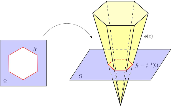
   Figure 5: Based on the level set method, the yield surface interface $f_{\Gamma}$ can be represented as the the zero level set of some higher-dimensional function $\phi(x)$.

   The signed distance function (see, for instance Figure 5) is defined as

   $$\phi(\widehat{\mathbf{x}},t)=\left\{\begin{array}[]{cl}d(\widehat{\mathbf{x}})&\text{ outside }f_{\Gamma}(\text{inadmissible stress})\\ 0&\text{ on }f_{\Gamma}(\text{yielding})\\ -d(\widehat{\mathbf{x}})&\text{ inside }f_{\Gamma}\text{ (elastic region)}\end{array}\right.,$$ (27)

   where $d(\widehat{\boldsymbol{x})}$ is the minimum Euclidean distance between any point $\boldsymbol{x}$ of $\Omega$ and the interface $f_{\Gamma}=\{\widehat{\boldsymbol{x}}\in\mathbb{R}^{2}|f(\widehat{\boldsymbol{x}})=0\}$, defined as:

   $$d(\widehat{\boldsymbol{x}})=\min\left(\left|\widehat{\boldsymbol{x}}-\widehat{\boldsymbol{x}}_{\Gamma}\right|\right).$$ (28)

   where $\boldsymbol{x}_{\Gamma}$ is the yielding stress for a given $\xi$. The signed distance function is obtained by solving the Eikonal equation $|\nabla^{\widehat{\boldsymbol{x}}}\phi|=1$ while prescribing the signed distance function as 0 at $\boldsymbol{x}\in f_{\Gamma}$ In the polar coordinate system, the Eikonal equation reads,

   $$(\frac{\partial{\phi}}{\partial{\rho}})^{2}+\frac{1}{\rho^{2}}((\frac{\partial{\phi}}{\partial{\theta}})^{2}=1.$$ (29)

   Note that the is a singularity at the polar coordinate of the $\pi-$ plane at $\rho=0$ and, hence, the origin point is not used as an auxiliary point to train the yield function. The Eikonal solution can be simply solved by a fast marching solver in the 2D polar coordinate.

   

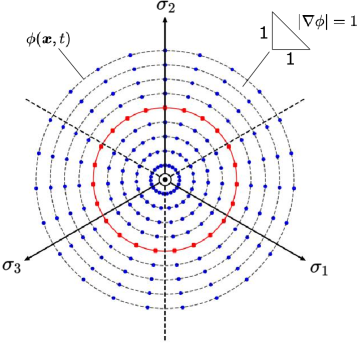
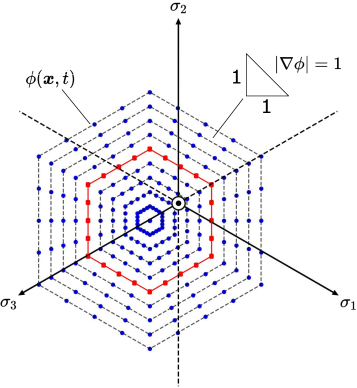
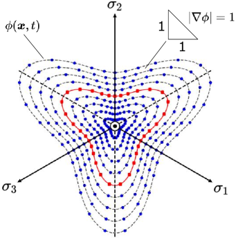
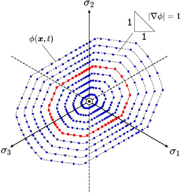
   Figure 6: Generation of auxiliary data points through level set re-initialization.The yield function level set $\phi(\boldsymbol{x},t)$ is created using a signed distance function. The initial yield surface points are given by the experimental results – a level set is constructed for every accumulated plastic strain $\bar{\epsilon}_{p}$ value in the data set. The isocontour curves represent the projection of the signed distance function level set on the $\pi$-plane.

   Figure 6 shows an example of solution a number of signed distance function converted from classical yield surfaces or deduced from direct numerical simulations.
   

2. Obtain the speed function to constitute Hamilton-Jacobi hardening of the yield function After we generate a sequence of signed distance function for different $\xi$, we might introduce an inverse problem to obtain the velocity function for the Hamilton-Jacobi equation that evolves the signed distance function. Recall that the Hamilton-Jacobi equation may take the following forms:

   $$\frac{\partial\phi}{\partial t}+\boldsymbol{v}\cdot\nabla^{\widehat{\boldsymbol{x}}}\phi=0,$$ (30)

   where $\boldsymbol{v}$ is the normal velocity field that defines the geometric evolution of the boundary and, in the case of plasticity, is chosen to describe the observed hardening mechanism. The velocity field is given by:

   $$\boldsymbol{v}=F\boldsymbol{n},$$ (31)

   where $F$ is a scalar function describing the magnitude of the boundary change and $\boldsymbol{n}=\nabla^{\widehat{\boldsymbol{x}}}\phi/|\nabla^{\widehat{\boldsymbol{x}}}\phi|$. Using $\nabla\phi\cdot\nabla\phi=|\nabla\phi|^{2}$ in Eq. (30), the level set Hamilton-Jacobi equation for stationary yield function can be simplified as,

   $$\frac{\partial\phi}{\partial t}+F|\nabla^{\widehat{\boldsymbol{x}}}\phi|=0.$$ (32)

   Note that $t$ is a pseudo-time and since the snapshot of $\phi$ we obtained from Step 1 remains a signed distance function, then $|\nabla^{\widehat{\boldsymbol{x}}}\phi|=1$. Next, we replace the pseudo-time $t$ with $\xi$. Assuming that the experimental data collected from different stress paths are collected data points $N$ times beyond the initial yielding point, each time with the same incremental plastic strain $\Delta\lambda$, then Step 1 will provide us a collection of signed distance function $\{\phi_{0},\phi_{1},....,\phi_{n+1}\}$ corresponding to $\{\xi_{0},\xi_{1},....,\xi_{n+1}\}$. Then, the corresponding velocity function can be obtained via finite difference, i.e.,

   $$F_{i}\approx\frac{\phi_{i}-\phi_{i+1}}{\xi_{i+1}-\xi_{i}},$$ (33)

   where $F_{i}(\rho,\theta)=F(\rho,\theta,\xi_{i})$ and $i=0,1,2,...,n+1$. By setting the signed distance function that fulfills Eq. 32 as the yield function, i.e., $f(\rho,\theta,\xi)=\phi(\rho,\theta,\xi)$ , we may use experimental data generated from the loading paths demonstrated in Fig. 4 to train a neural network to predict a new yield function or velocity function for an arbitrary $\xi$ that represent the history of the strain (see Figure 7).

   

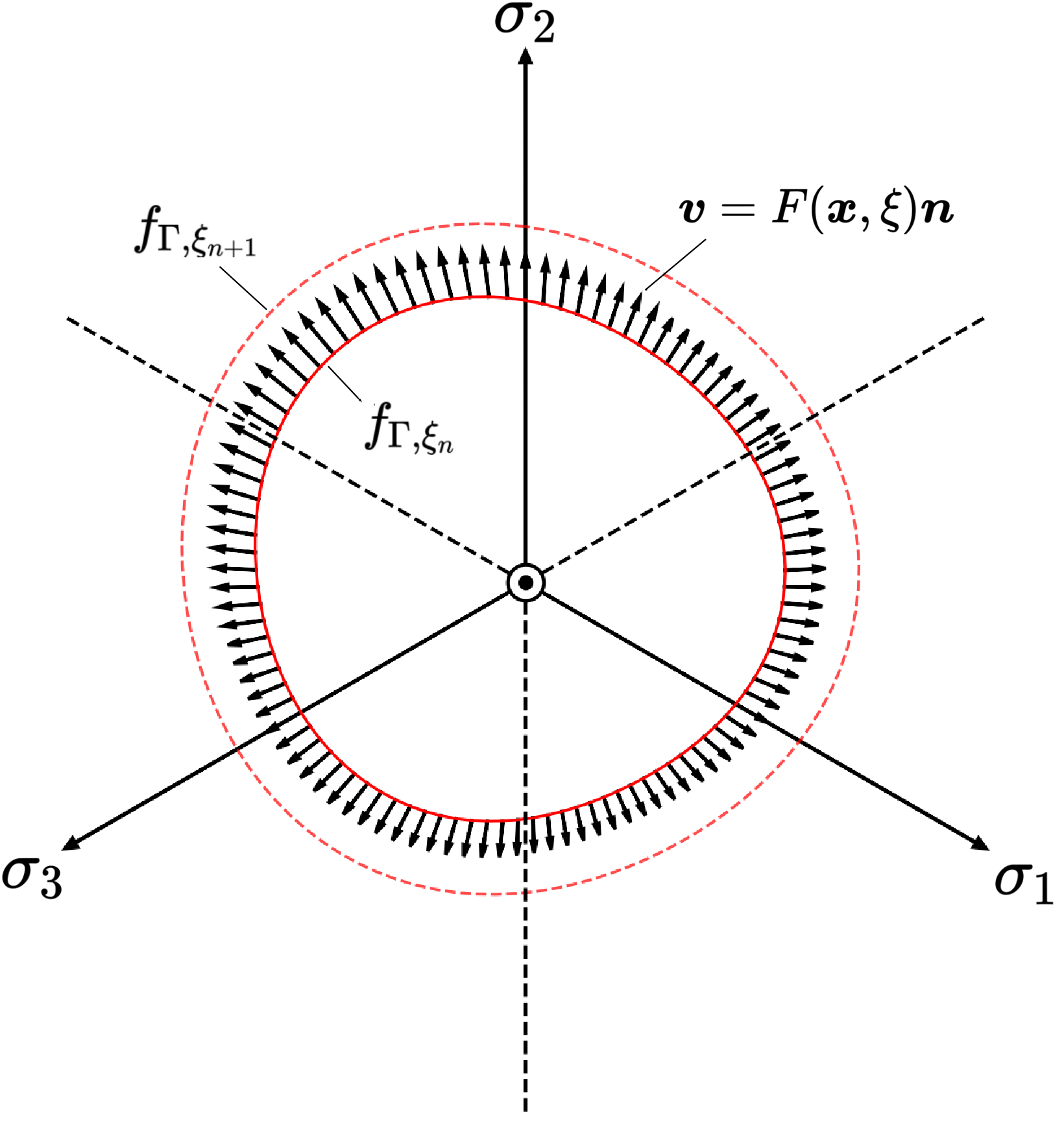
   Figure 7: The evolution of the yield surface $f_{\Gamma}$ is connected to a level set $\phi(\boldsymbol{x},\xi)$ extension problem. The velocity field of the Hamilton-Jacobi equation (32) emulates the material hardening law. The yield surface evolution and the velocity field are inferred from the data through the neural network training.

More importantly, we show that the evolution of the yield function can be modeled as a level set evolving according to a Hamilton-Jacobi equation. This knowledge may open up many new possibilities to capture hardening without any hand-crafted treatment. To overcome the potential cost to solve the Hamilton-Jacobi equation, we will introduce a supervised learning procedure to obtain the updated yield function for a given strain history represented by the internal variable $\xi$ without explicitly solving the Hamilton-Jacobi equation (see the next sub-sections). Consequently, this treatment will enable us to create a generic elasto-plasticity framework that can replace the hard-crafted yield functions and hardening laws without the high computational costs and the burden of repeated modeling trial-and-errors.

2.3.4 Training yield function with associative plastic flow

Assuming an associative flow rule, the generalized Hooke’s law utilizing a yield function neural network approximator $\widehat{f}$ can be written in rate form as:

$$\dot{\boldsymbol{\sigma}}=\boldsymbol{c}^{\mathrm{e}}:\left(\dot{\boldsymbol{\epsilon}}-\dot{\lambda}\frac{\partial\widehat{f}}{\partial\boldsymbol{\sigma}}\right).$$ (34)

And in incremental form, the predictor-corrector scheme is written as:

$$\boldsymbol{\sigma}_{n+1}=\boldsymbol{\sigma}_{n+1}^{\mathrm{tr}}-\Delta\lambda\boldsymbol{c}_{n+1}^{\mathrm{e}}:\left.\frac{\partial\widehat{f}}{\partial\boldsymbol{\sigma}}\right|_{n+1},$$ (35)

where

$$\boldsymbol{\sigma}_{n+1}^{\mathrm{tr}}=\boldsymbol{\sigma}_{n}+\boldsymbol{c}_{n+1}^{\mathrm{e}}:\Delta\boldsymbol{\epsilon}=\boldsymbol{c}_{n+1}^{\mathrm{e}}:\boldsymbol{\epsilon}_{n+1}^{\mathrm{e}\operatorname{tr}},\quad\boldsymbol{\epsilon}_{n+1}^{\mathrm{etr}}=\boldsymbol{\epsilon}_{n}^{\mathrm{e}}+\Delta\boldsymbol{\epsilon}.$$ (36)

The strain and stress tensor predictors can be written in spectral form as follows:

$$\boldsymbol{\sigma}_{n+1}^{\mathrm{tr}}=\sum_{A=1}^{3}\sigma_{A,n+1}^{\mathrm{tr}}\boldsymbol{n}_{n+1}^{\operatorname{tr}(A)}\otimes\boldsymbol{n}_{n+1}^{\operatorname{tr}(A)},\qquad\boldsymbol{\epsilon}_{n+1}^{\mathrm{etr}}=\sum_{A=1}^{3}\epsilon_{A,n+1}^{\mathrm{etr}}\boldsymbol{n}_{n+1}^{\operatorname{tr}(A)}\otimes\boldsymbol{n}_{n+1}^{\operatorname{tr}(A)}.$$ (37)

The predictor-corrector scheme can be rewritten in spectral form, omitting the subscript $(n+1)$

$$\sum_{A=1}^{3}\sigma_{A}\boldsymbol{n}^{(A)}\otimes\boldsymbol{n}^{(A)}=\sum_{A=1}^{3}\sigma_{A}^{\operatorname{tr}}\boldsymbol{n}^{\operatorname{tr}(A)}\otimes\boldsymbol{n}^{\operatorname{tr}(A)}-\Delta\lambda\sum_{A=1}^{3}\left(\sum_{B=1}^{3}a_{AB}^{\mathrm{e}}\widehat{f}_{B}\right)\boldsymbol{n}^{(A)}\otimes\boldsymbol{n}^{(A)}$$ (38)

$$\boldsymbol{n}^{(A)}\otimes\boldsymbol{n}^{(A)}=\boldsymbol{n}^{\operatorname{tr}(A)}\otimes\boldsymbol{n}^{\operatorname{tr}(A)}$$ (39)

By assuming that the plastic flow obeys the normality rule, we may use the observed plastic flow from the data to regularize the shape of the evolving yield function. To do so, we will leverage the fact that we have already obtained an elastic energy functional from the previous training. The plastic deformation mode can then be obtained by the difference between the trial and the true Cauchy stress at each incremental step where the data are recorded in an experiment or directed numerical simulations, i.e.,

$$\sigma_{A} =\sigma_{A}^{\mathrm{tr}}-\Delta\lambda\sum_{B=1}^{3}a_{AB}^{\mathrm{e}}f_{B},$$ (40)

$$f_{A} =\partial f/\partial\sigma_{A}=\frac{\epsilon_{A}^{\mathrm{etr}}-\epsilon_{A}^{\mathrm{e}}}{\Delta\lambda}\text{ for }A=1,2,3.$$

At every incremental step of the data generating simulations, we have information on the total strain and total stress of the material. Having the knowledge of the underlying hyperelastic model, we can utilize an inverse mapping to estimate the elastic strain that would correspond to the current total stress, if there was no plasticity. Thus, we can post-process the available data to gather the plastic flow information necessary for the network training.

The quantities $f_{1},f_{2},f_{3}$ correspond to the amount of plastic flow in the principal directions $A=1,2,3$. A neural network approximator of the yield function should have adequately accurate stress derivatives that are necessary for the implementation of the return mapping algorithm, discussed in Section LABEL:sec:return_mapping_algorithm, and so as to provide an accurate plastic flow, in the case of associative plasticity. The normalized plastic flow direction vector $\boldsymbol{\overline{f}}_{\text{norm}}$ can be defined as

$$\boldsymbol{\overline{f}}_{\text{norm}}=\langle\widehat{f}_{1},\widehat{f}_{2},\widehat{f}_{3}\rangle/\|\langle\widehat{f}_{1},\widehat{f}_{2},\widehat{f}_{3}\rangle\|,$$ (41)

and holds information about the yield function shape in the $\pi$-plane.

In the case of the simple MLP feed-forward network, the network can be seen as an approximator function $\widehat{f}=\widehat{f}(\rho,\theta,\xi|\boldsymbol{W},\boldsymbol{b})$ of the true yield function level set $f$ with input the Lode’s coordinates $\rho$, $\theta$, and the hardening parameter $\xi$, parametrized by weights $\boldsymbol{W}$ and biases $\boldsymbol{b}$. A classical training objective, following an $L_{2}$ norm, would only constrain the predicted yield function values. The corresponding training objective is to minimize the discrepancy measured at $N$ number of sample points $(\widehat{\boldsymbol{x}},\xi)\in\mathbb{S}\times\mathbb{R}^{1}$ reads,

$$\boldsymbol{W}^{\prime},\boldsymbol{b}^{\prime}=\operatorname*{argmin}_{\boldsymbol{W},\boldsymbol{b}}\left(\frac{1}{N}\sum_{i=1}^{N}\gamma_{7}\left\lVert f_{i}-\widehat{f}_{i}\right\rVert^{2}_{2}\right),$$ (42)

where $f_{i}=f((\widehat{\boldsymbol{x}}_{i},\xi_{i})$ and $\widehat{f}_{i}=f((\widehat{\boldsymbol{x}}_{i},\xi_{i})$. A second training objective can be modeled after an $H_{1}$ norm, constraining both $f$ and its first derivative with respect to the stress state $\sigma_{1},\sigma_{2},\sigma_{3}$. For a neural network aprroximator parametrized as $\overline{f}=\overline{f}(\sigma_{1},\sigma_{2},\sigma_{3},\xi|\boldsymbol{W},\boldsymbol{b})$ using the principal stresses as inputs, this training objective for the training samples $i\in[1,...,N]$ would have the following form:

$$\boldsymbol{W}^{\prime},\boldsymbol{b}^{\prime}=\operatorname*{argmin}_{\boldsymbol{W},\boldsymbol{b}}\left(\frac{1}{N}\sum_{i=1}^{N}\left(\gamma_{7}\left\lVert f_{i}-\overline{f}_{i}\right\rVert^{2}_{2}+\sum_{A=1}^{3}\gamma_{8}\left\lVert\frac{\partial f_{i}}{\partial\boldsymbol{\sigma_{A}}_{i}}-\frac{\partial\overline{f}_{i}}{\partial\boldsymbol{\sigma_{A}}_{i}}\right\rVert^{2}_{2}\right)\right).$$ (43)

Utilizing an equivalent representation of the stress state with Lode’s coordinates in the $\pi$-plane, the above training objective can further be simplified. The normalized flow direction vector $\boldsymbol{\overline{f}}_{\text{norm}}$ in Lode’s coordinates can solely be described using an angle $\theta_{f}$ since the vector has a magnitude equal to unity. To constrain the flow direction angle, we modify the loss function of this higher order training objective by adding a distance function metric between two rotation tensors $\boldsymbol{R}_{\theta,i}$, $\boldsymbol{R}_{\widehat{\theta},i}$, corresponding to $\theta_{f,i}$ and $\widehat{\theta}_{f,i}$ – the flow vector directions in the $\pi$-plane for the data and approximated yield function respectively for the $i$-th sample. The two rotation tensors belong to the Special Orthogonal Group, SO(3) and the metric is based on the distance from the identity matrix. For the $i$-th sample, the rotation related term can be calculated as:

$$\overline{\Phi}_{i}=\left\|\boldsymbol{I}-\boldsymbol{R}_{\theta,i}\left(\boldsymbol{R}_{\widehat{\theta},i}\right)^{T}\right\|_{F}=\sqrt{2\left[3-\operatorname{tr}\left[\boldsymbol{R}_{\theta,i}\left(\boldsymbol{R}_{\widehat{\theta},i}\right)^{T}\right]\right]},$$ (44)

where $\|\cdot\|_{F}$ is the Frobenius norm. For a neural network aprroximator parametrized via the Lode’s coordinates as input, i.e. $\widehat{f}=\widehat{f}(\rho,\theta,\xi|\boldsymbol{W},\boldsymbol{b})$, the Sobolev training objective for the training samples $i\in[1,...,N]$ reads,

$$\boldsymbol{W}^{\prime},\boldsymbol{b}^{\prime}=\operatorname*{argmin}_{\boldsymbol{W},\boldsymbol{b}}\left(\frac{1}{N}\sum_{i=1}^{N}\left(\gamma_{7}\left\lVert f_{i}-\widehat{f}_{i}\right\rVert^{2}_{2}+\gamma_{9}\overline{\Phi}_{i}\right)\right),$$ (45)

where we minimize both the discrepancy of the yield function and the direction of the gradient in the stress space.