Improving Audio Anomalies Recognition Using Temporal Convolutional Attention Networks

Abstract

Anomalous audio in speech recordings is often caused by speaker voice distortion, external noise, or even electric interferences. These obstacles have become a serious problem in some fields, such as high-quality dubbing and speech processing. In this paper, a novel approach using a temporal convolutional attention network (TCAN) is proposed to tackle this problem. The use of temporal conventional network (TCN) can capture long range patterns using a hierarchy of temporal convolutional filters. To enhance the ability to tackle audio anomalies in different acoustic conditions, an attention mechanism is used in TCN, where a self-attention block is added after each temporal convolutional layer. This aims to highlight the target related features and mitigate the interferences from irrelevant information. To evaluate the performance of the proposed model, audio recordings are collected from the TIMIT dataset, and are then changed by adding five different types of audio distortions: gaussian noise, magnitude drift, random dropout, reduction of temporal resolution, and time warping. Distortions are mixed at different signal-to-noise ratios (SNRs) (5dB, 10dB, 15dB, 20dB, 25dB, 30dB). The experimental results show that the use of proposed model can yield better classification performances than some strong baseline methods, such as the LSTM and TCN based models, by approximate 3$\sim$ 10% relative improvements.

Index Terms—  Audio anomaly classification, temporal convolutional network, self-attention

1 Introduction

Assessing the quality of audio signals is an important consideration in many audio and multimedia applications, such as speech recognition, high-quality music recording, and machine fault detection. By now, there have been some studies in audio quality assessment [1, 2, 3, 4]. Fu et al.[2] developed a non-intrusive speech quality evaluation model to predict PESQ scores using a BLSTM model. Avila et al., [3] investigated the applicability of three neural network-based approaches for non-intrusive audio quality assessment based on mean opinion score(MOS) estimation [5]. These previous studies mainly focused on quality estimations of audio recordings by predicting a quality score. To our knowledge, few investigated how to identify what type an anomalous distortion is. Moreover, identifying the type of audio anomalies will be useful to anomaly detection and audio quality enhancement, which could benefit various fields in industry. To tackle the audio anomalies classification, it is highly desirable not only to find out whether there exist audio anomalies in audio recordings, but also to identify which type an audio distortion belongs to.

In this work, a Temporal Convolutional Attention Network [6] is proposed and investigated. This is because TCNs have advantages in two aspects. Firstly, TCNs use 1D dilated convolutions [7] to flexibly enlarge their receptive field through increasing their dilation rate. This enables TCN to process long-term sequences by using a wider part of the input data to contribute to the output [8]. Secondly, unlike the RNN-based methods, its computation is performed layer-wise and its weights at every time-step are updated simultaneously [6]. By now, there have been already some applications of TCN in activity detection [9, 10], language processing [11] and event detection [12]. However, it was found in our experiments that the use of TCN did not show satisfying performances on audio anomalies classification in some conditions, e.g. the SNR of distortion corrupted signals is relatively low or high. For this reason, an attention mechanism is integrated into TCN, as attention [13, 14, 15] exhibits a better balance between the ability to model long-range dependencies and the computational and statistical efficiency. Unlike a previous study [16] using an attention block after a TCN block, our work goes deeper into the TCN block by inserting a self attention layer after each 1D conventional layer. The related details of our model will be introduced in the following sections.

The rest of paper is organised as follows: Section 2 introduces the proposed model architecture in detail. Section 3 depicts the used dataset and experimental set up. Section 4 presents and analyses the obtained results, and finally the conclusion and future work are given in Section 5.

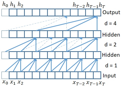
(a)

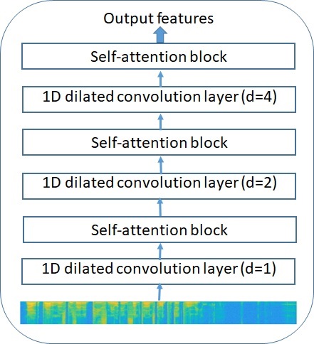
(b)

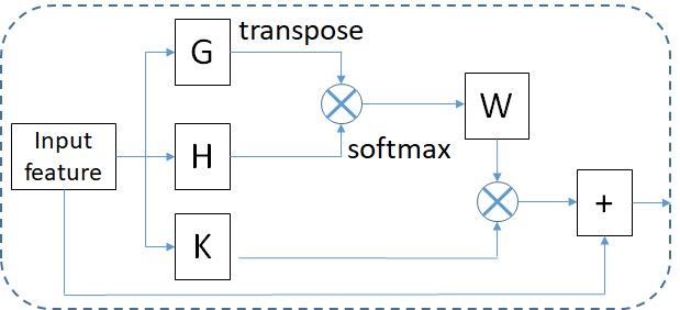
(c)

Fig. 1: Architecture of the Temporal Convolutional Attention Network (TCAN): (a) A 3-layer dilated causal convolution; (b) The basic structure of TCAN; (c) Self-attention block.

2 Model Architecture

Given an input audio feature sequence $\textbf{x}=\{x_{0},\cdots,x_{T}\}$, our aim is to identify the type of audio anomalous distortions $\textbf{A}=\{a_{i},\cdots,a_{M}\}$ in recordings, and M is the number of distortion classes. As aforementioned in Section 1, the use of TCN is to collect dependencies over long spans using dilated convolutional layers. Figure 1 shows the architecture of proposed approach using the temporal convolutional attention network. Figure 1(a) illustrates the structure of a dilated causal convolution with dilation factors $d=\{1,2,4\}$ and filter size $k=3$. Figure 1(b) shows the temporal convolutional attention networks expanded by inserting an attention block between two convolutional layers of a TCN, and Figure 1(c) shows the structure a self-attention block.

2.1 Temporal Convolutional Network

As shown in Figure 1(a), the TCN relies on 1D dilated convolutional layers stacked hierarchically. For a 1D sequence input $\textbf{x}\in\Re^{n}$ and a filter $f:\{0,\cdots,k-1\}\rightarrow\Re$, the dilated convolution operation $F$ on element $s$ of the sequence is defined as:

$$F(s)=\Sigma_{i=0}^{k-1}f(i)\cdot x_{s-d\cdot i}$$ (1)

where $d$ is the dilation factor, $k$ is the filter size, and $s-d\cdot i$ accounts for the direction of the past[6]. It is clear that the TCN is controlled by two parameters, dilation factor ($d$) and filter size ($k$). Dilation is equivalent to introducing a fixed step between every $d$ adjacent filter taps. Increasing its value can lead to the increment of the depth of the network (i.e., $d=O(2^{i})$ at level $i$ of the network). When $d=1$, a dilated convolution reduces to a regular convolution. Using larger dilation enables an output at the top level to represent a wider range of inputs, thus effectively expanding the receptive field of convolutional layers[6]. For choosing larger filter sizes $k$, the effective history of one such layer is $(k-1)d$. With above designs, the TCN model is thus able to take similar inputs and produce similar outputs as RNNs while it is efficient taking advantage of convolution architectures.

2.2 Temporal Convolutional Attention Network

In comparison with the basic structure of TCN, the TCAN aims to find which features are more relevant to the recognition target and which are less or not when search through observed long data streams. As shown in figure 1(b), the basic TCN structure is expanded by adding a self-attention block after a 1D dilated convolutional layer.

The architecture of the used self-attention unit [17] is shown in Figure 1(c). The input features are transformed into $G$ and $H$ via 1D convolution, and then generate the attention weights $W$ from $G$ and $H$ by

$$W=f_{softmax}(G^{T}H)$$ (2)

where $f_{softmax}$ denotes the softmax function. After that, the weighted features $W^{T}K$ are obtained, where $K$ is another set of features transformed from 1D convolution. The output features is the sum of the weighted features and original inputs.

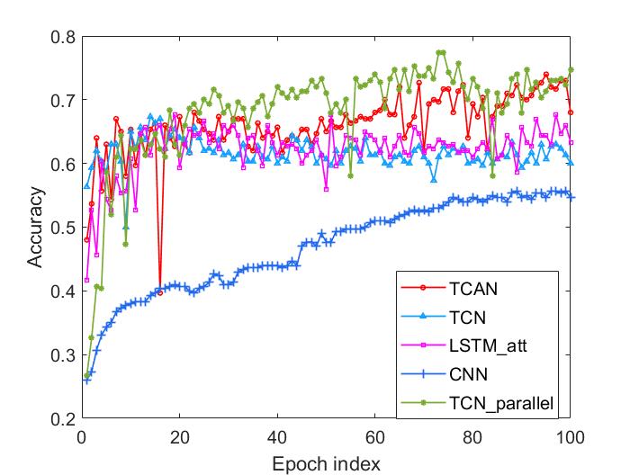
(a) SNR=5dB

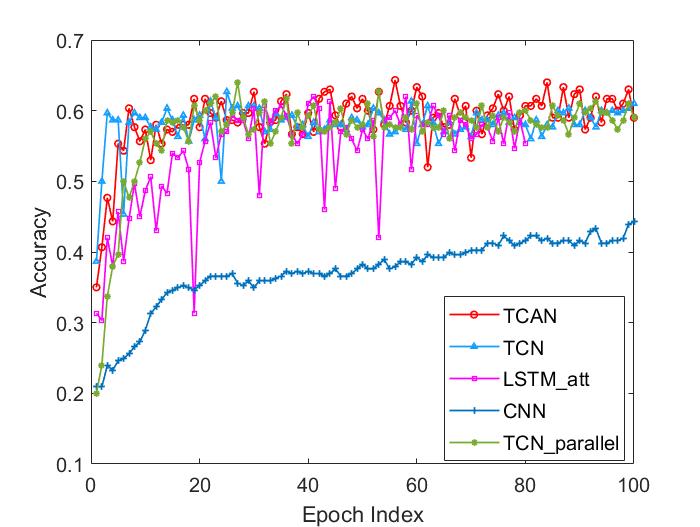
(b) SNR=10dB

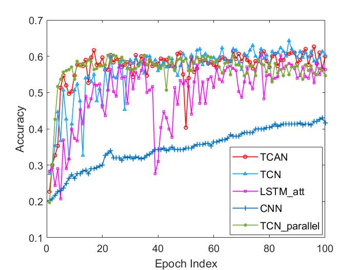
(c) SNR=15dB

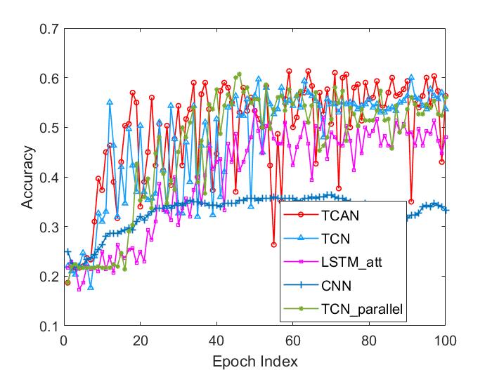
(d) SNR=20dB

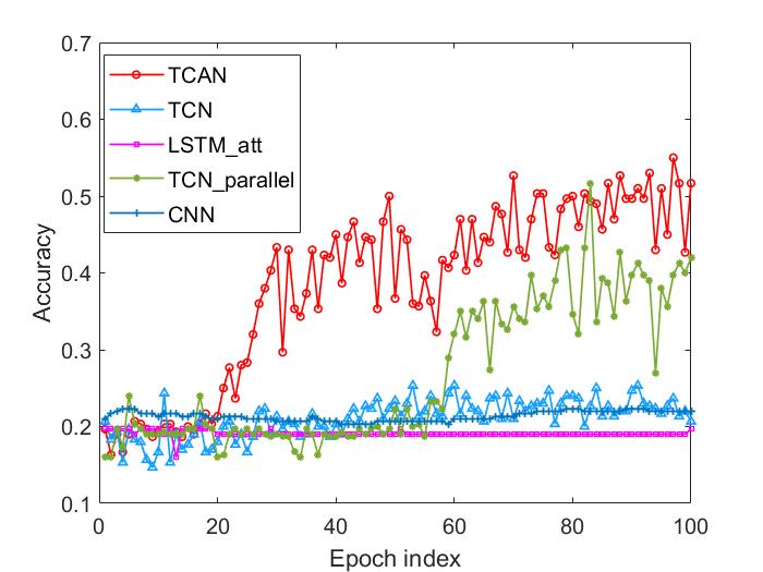
(e) SNR=25dB

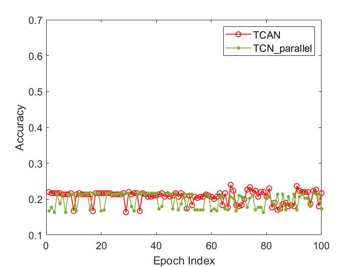
(f) SNR=30dB

Fig. 2: Accuracy comparisons of audio anomalous distortion classification when implementing TCAN and four baseline methods in the condition of different SNRs.

3 Data and Experimental Set Up

3.1 Data

In our experiments, the TIMIT dataset [18] was used. 3436 recordings, longer than 2.5 seconds, were selected from the original TIMIT training set and utilized as the training data in this paper. Meanwhile, 600 recordings selected from the original TIMIT test set in the same condition were used for evaluation. The audio anomalous distortion classes were generated by changing the original signals in five ways [19],

Random time warping (Class1):

The time warping is controlled by the number of speed changes and the maximal ratio of max/min speed.

Pooling time series (Class2):

Reduce the temporal resolution without changing the length.

Dropouting values of time series (Class3):

Some random time points in time series are dropped out.

Drifting the value of time series (Class4):

The values of time series are drifted from its original values randomly and smoothly.

Adding random noise to time series (Class5):

The noise added to every time point of a time series is independent and identically distributed.

As the work in this paper focuses on the distortions assumed to be caused by speakers, external natural sounds were not used as noise signals. The four distortion classes (Class 1 $\sim$ 4) except Class5 are made by only changing the characters of audio signals, such as temporal resolution and speaking speed. In order to evaluate the robustness of the proposed approach, the recordings corrupted by the five types of distortions are generated at six signal-to-noise ratio (SNR) levels (5dB, 10dB, 15dB, 20dB, 25dB, 30dB). The larger SNR is, the more difficult it is to identify audio anomalies.

In all experiments, filter-bank vectors are used to represented input audio features. 2-second audio data is selected from each audio recording and segmented using a 32-ms sliding window with a 16-ms shift. After conducting a 512-point FFT, each segment is converted into a 40D vector with filter banks.

3.2 Structure Configuration and Implementation

In the experiments, the proposed model architecture contains two parts. The first nine layers consisting of 1D dilated CNN and attention layers are used to build TCAN, and the last two layers are fully connected layers used as a classifier. The dimension of input frame vector is 40, and 64 kernels ($k=$6) are used in four 1D dilated CNN layers with $d=\{1,2,4,8\}$.

As a comparison, besides the proposed approach (TCAN), the related experiments were also conducted using another four baseline methods: TCN$\_$parallel[16], TCN[6], CNN[20], and, LSTM$\_$att[21]. The method of TCN$\_$parallel connects three temporal convolutional networks (TCNs) in parallel. Each of TCN is followed by an attention layer and their output are then concatenated before sending to a MLP based classifier. The dilation value (d) and kernel size (k) in TCN$\_$parallel are set to 8 and 6, respectively. The TCN baseline is implemented relying on the model structure given in [6], where its $d$ and $k$ are set to be 32 and 6, respectively. The baseline method of LSTM$\_$att makes use of the Bi-directional LSTM [22] and an attention mechanisms to capture the long-term dependencies. The dimensionality of the output space of the LSTM$\_$att is 200. The baseline method of CNN, originally used for sentence classification, is used for audio recording distortion classification, and its filter number is set to 64.

In all experiments, Adam [23] was used as an optimiser and the initial learning rate was set to 0.001 with 0.95 decay every epoch. Classification accuracy is used as a metric in all experiments to evaluate performances of the proposed approach and four baseline methods.

4 Results Analysis

Figure 2(a)$\sim$2(f) show audio distortion recognition using the proposed approach (TCAN) and four baseline methods in the condition of six SNR. Figure 2(f) only shows the accuracy curves obtained using TCAN and TCN$\_$parallel when SNR is 30dB. This is because other methods have failed to recognise the type of audio distortions when SNR is 25dB, and it is thus unnecessary to run them again when SNR is 30dB. By the first five figures, it can be found that the use of TCAN can clearly outperform LSTM$\_$att and CNN in all SNR conditions. This might be related to the following factors. The CNN relies on kernel size and focuses more on local dependencies in comparison with the use of TCN. Although the LSTM takes into account long spans, the currently observed signals still play relatively important roles than historical observations. The structure of TCN tries to mitigate this impact by viewing all features in a data stream more equally. Moreover, the use of dilation can further expand the search for longer dependencies, and the learned information can be passed to a classifier from bottom to top via a hierarchical structure. This might be effective to enable the TCN to capture both long and short term dependencies of data streams.

In addition, compared to TCN, the proposed approach can yield better performances for most SNR cases. The possible reason is the use of an attention mechanism. The structure of TCN aims to collect long range features, but not all the collected features are useful to the task. Some of them might be irrelevant features and even interferences. The use of attention mechanism can mitigate this impact by allocating different weights to target relevant and irrelevant features.

In comparison with TCN$\_$parallel, it seems that TCAN works better when SNR is increased. The reason might be related to where to use attention mechanism. As audio distortions become quite weak in the condition of high SNR (e.g. SNR=25dB), highlighting target relevant information as early as possible might be useful to mitigate the interferences from strong speech signals. Following the assumption, the use of TCAN can go deeper than TCN$\_$parallel to search for target relevant features to reduce possible information loss.

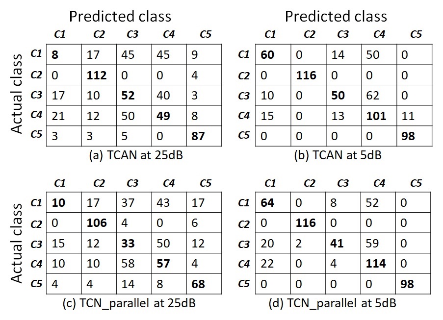
Fig. 3: Confusion matrix for audio anomalies classification using TCAN and TCN$\_$parallel when SNR is 5dB and 25dB.

Figure 3 illustrates four confusion matrix tables obtained by using TCAN and TCN$\_$parallel in the conditions of SNR$=$5dB and SNR$=$25dB, respectively. In the condition of 5dB, both methods can yield good and similar recognition performances. In the condition 25dB, TCAN can better distinguish the five types of audio distortions than TCN$\_$parallel. When SNR is 25dB, the anomalous distortions in recordings are much smaller than those at 5dB. This makes class1(C1) be more easily classified as incorrect classes, such as class3(C3) and class4(C4), than that at 5dB. In the same condition, both methods can well recognise two types of audio distortions, class2(C2) and class4(C4), but failed to recognise class1(C1). For the two cases, the possible reason might be related to what parts of input audio signals are changed. For the audio distortion caused by ”random time warping(C1)”, it has mainly effect on some specific frequencies. This case might also occur within an utterance if the tune of words or phrases is normally changed by a speaker. This might bring some extra interferences and make it difficult to learn distinct features when speech signals are dominant. For “pooling time series(C2)” and “adding random noise(C5)”, both of them can add distortions on the whole data sequence, and thus change the feature values in both time and frequency domains simultaneously. The changes caused by the two types of distortion might be able to bring some salient differences, which enable them to be found more easily than other distortion classes.

d=1	d=2	d=4	d=8	d=16	d=32	d=64
48.6	54.3	52.3	53.6	55.3	56.3	52.3

Table 1: Classification accuracy (%) with different dilation values (SNR=25dB, k=6).

Table 1 shows the change of classification accuracy when different dilation (d) is set. It seems that there is a weak tendency that accuracy is slightly better when increasing $d$. The possible reason might be larger $d$ is able make the model learn information from a longer range.

5 Conclusion and Future Work

A novel structure for audio distortion classification was designed by using the temporal convolutional attention network (TCAN). It can well distinguish five different types of audio distortions in condition of different SNRs. Moreover, the obtained results have shown its robustness to in comparison with several strong baseline methods, especially when SNR is relatively low (5dB) or high (25dB).

In future, work in three aspects will be taken into account. Firstly, some advanced neural network technologies will be used to assess audio quality. Secondly, the classification technologies will be evaluated on large-sized speech datasets and in various acoustic conditions. Thirdly, more audio distortion types and model configurations will be also evaluated to make the system work in some practical applications.

Acknowledgements
This work was supported by Innovate UK Grant number 104264 MAUDIE.

References

- [1] Constantin Spille, Stephan Ewert, Birger Kollmeier, and Bernd Meyer, “Predicting speech intelligibility with deep neural networks,” Computer Speech and Language, vol. 48, pp. 51–66, October 2017.
- [2] Szu-Wei Fu, Yu Tsao, Hsin-Te Hwang, and Hsin-Min Wang, “Quality-net: An end-to-end non-intrusive speech quality assessment model based on blstm,” in Interspeech, 2018, pp. 3168–3172,.
- [3] Neil Shah, Hemant Patil, and Meet Soni, “Time-frequency mask-based speech enhancement using convolutional generative adversarial network,” in Conference: Asia-Pacific Signal and Information Processing Association Annual Summit and Conference, August 2018.
- [4] Meet H. Soni and Hemant A. Patil, “Novel deep autoencoder features for non-intrusive speech quality assessment,” in The 24th European Signal Processing Conference (EUSIPCO), 2016, pp. 2315–2319.
- [5] C. Robert Streijl, Stefan Winkler, and S. David Hands, “Mean opinion score (mos) revisited: methods and applications, limitations and alternatives,” Multimedia Systems, vol. 22, pp. 213–227, 2016.
- [6] Shaojie Bai, J. Kolter, and Vladlen Koltun, “An empirical evaluation of generic convolutional and recurrent networks for sequence modeling,” https://arxiv.org/abs/1803.01271, 03 2018.
- [7] Shaojie Bai, J. Zico Kolter, and Vladlen Koltun, “Convolutional sequence modeling revisited,” in ICLR, 2018.
- [8] van den A. Oord, S. Dieleman, H. Zen, K. Simonyan, O. Vinyals, A. Graves, N. Kalchbrenner, A. Senior, and K. Kavukcuoglu, “Wavenet a generative model for raw audio,” https://arxiv.org/abs/1609.03499, 2016.
- [9] Colin Lea, D. Michael Flynn, Rene Vidal, Austin Reiter, and D. Gregory Hager, “Temporal convolutional networks for action segmentation and detection,” in CVPR, 2017, pp. 156–165.
- [10] A. Yazan Farha and Jurgen Gall, “Ms-tcn: Multi-stage temporal convolutional network for action segmentation,” in CVPR, 2019, pp. 3575–3584.
- [11] Sawsan Alqahtani, Ajay Mishra, and Mona Diab, “Efficient convolutional neural networks for diacritic restoration,” in EMNLP, 2019, pp. 1442–1448.
- [12] Yangdong He and Jiabao Zhao, “Temporal convolutional networks for anomalydetection in time series,” in Journal of Physics, 2019, pp. 1–6.
- [13] Ashish Vaswani, Noam Shazeer, Niki Parmar, Jakob Uszkoreit, Llion Jones, Aidan N. Gomez, Lukasz Kaiser, and Illia Polosukhin, “Attention is all you need,” 2017, pp. 6000–6010.
- [14] Jianpeng Cheng, Li Dong, and Mirella Lapata, “Long short-term memory-networks for machine reading,” in Proceedings of the 2016 Conference on Empirical Methods in Natural Language Processing. Nov. 2016, pp. 551–561, Association for Computational Linguistics.
- [15] Ankur Parikh, Oscar Täckström, Dipanjan Das, and Jakob Uszkoreit, “A decomposable attention model for natural language inference,” in Proceedings of the 2016 Conference on Empirical Methods in Natural Language Processing. Nov. 2016, pp. 2249–2255, Association for Computational Linguistics.
- [16] Junyao Huang, Chenhui Lu, Guolou Ping, Lin Sun, and Xiaojun Ye, “Tcn-att: A non-recurrent model for sequence-based malware detection,” Advances in Knowledge Discovery and Data Mining, vol. 12085, pp. 178 – 190, 2020.
- [17] Kuldeep Purohit and Rajagopalan, “Region-adaptive dense network for efficient motion deblurring,” arXiv:1903.11394, 2019.
- [18] J. Garofolo, Lori Lamel, W. Fisher, Jonathan Fiscus, D. Pallett, N. Dahlgren, and V. Zue, “Timit acoustic-phonetic continuous speech corpus,” Linguistic Data Consortium, November 1992.
- [19] ARUNDO, “https//tsaug.readthedocs.io/en/stable/,” accessed: 01.09.2020.
- [20] Ye Zhang and C. Byron Wallace, “A sensitivity analysis of convolutional neural networks for sentence classification,” in Proceedings of the The 8th International Joint Conference on Natural Language Processing, 2017, pp. 253–263.
- [21] Beakcheol Jang, Myeonghwi Kim, Gaspard Harerimana, Sang-ug Kang, and Jong Wook Kim, “Bi-lstm model to increase accuracy in text classification: Combining word2vec cnn and attention mechanism,” Applied Sciences, pp. 1–14, 08 2020.
- [22] F. Gers, N. Schraudolph, and J. Schmidhuber, “Learning precise timing with lstm recurrent networks,” pp. 115–143, 2002.
- [23] Diederik Kingma and Jimmy Ba, “Adam: A method for stochastic optimization,” in Proceedings of International Conference on Learning Representations, 2014, pp. 253–263.