Modeling Rydberg Gases using Random Sequential Adsorption on Random Graphs

Abstract

The statistics of strongly interacting, ultracold Rydberg gases are governed by the interplay of two factors: geometrical restrictions induced by blockade effects, and quantum mechanical effects. To shed light on their relative roles in the statistics of Rydberg gases, we compare three models in this paper: a quantum mechanical model describing the excitation dynamics within a Rydberg gas, a Random Sequential Adsorption (RSA) process on a Random Geometric Graph (RGG), and a RSA process on a Decomposed Random Intersection Graph (DRIG). The latter model is new, and refers to choosing a particular subgraph of a mixture of two other random graphs. Contrary to the former two models, it lends itself for a rigorous mathematical analysis; and it is built specifically to have particular structural properties of a RGG. We establish for it a fluid limit describing the time-evolution of number of Rydberg atoms, and show numerically that the expression remains accurate across a wider range of particle densities than an earlier approach based on an RSA process on an Erdös–Rényi Random Graph (ERRG). Finally, we also come up with a new heuristic using random graphs that gives a recursion to describe a normalized pair-correlation function of a Rydberg gas. Our results suggest that even without dissipation, on long time scales the statistics are affected most by the geometrical restrictions induced by blockade effects, while on short time scales the statistics are affected most by quantum mechanical effects.

I Introduction

Ultra cold gases with atoms in highly excited states—Rydberg atoms—have attracted substantial interest over recent years for their applications in quantum computing and the study of nonequilibrium phase transitions [1, 2, 3, 4, 5]. Rydberg atoms are significant because a powerful Van der Waals interaction causes the atoms to feel mutual interactions over mesoscopic distances (tens of micrometers); a single Rydberg atom in a gas causes energy level shifts that make it impossible for neighboring atoms to excite to the same state. This dipole blockade leads to intriguing networked and complex spatial behavior, resulting in effects linked to fundamental problems in condensed matter physics [1, 6, 3, 7, 8, 9, 10, 11]. For an overview of applications, we refer the interested reader to [12].

The computational effort to accurately simulate the quantum mechanical behavior of Rydberg gas grows exponentially in the number of atoms. Precise numerical calculations are therefore commonly limited to the order of ten atoms, although approximations can be used to raise this number [13, 14, 15]. Theoretically, there has therefore been focus on models that are more tractable: for example, rate equations were proposed to describe the Rydberg gas [16, 17, 18]; the Mandel Q parameter was studied under reversible dynamics [19] and using RSA processes on ERRGs [20]; and the physics of Rydberg atoms has e.g. been related to a nonlinear optical polarizability model [21] as well as glassy soft-matter models [22, 23]. Also, ties to classical statistics can be found in related Ising models, dissipative approaches, and open quantum systems [24, 25, 26, 27].

The focus of this paper is on a new, generalized variant of the RSA process described in [20], which is setup to mimic the Rydberg gas even more closely. Recall that the canonical, continuum two-dimensional RSA process is that of randomly throwing disks of radius $r>0$ one by one in a two-dimensional box, and in such a way that the disks do not overlap [28, 29]. The spatial correlations in RSA processes are notoriously challenging to analyze on such continuum, there being only an exception for the one-dimensional case (a line) [30]. To bypass this mathematical difficulty, one may opt to conduct RSA on a random graph instead; and in fact, such approach was used to provide a closed-form expression for the Mandel Q parameter of a Rydberg gas as well as a description of the average number of Rydberg atoms over time [20]. The comparison to experiments there shows that such model is capable of describing the statistics of a Rydberg gas accurately.

This accuracy is surprising in light of the facts that RSA and random graphs both belong to the realm of classical probability theory, and the vertices of e.g. the ERRG [31] have no property corresponding to a physical position of a particle. This raises two fundamental questions. First, if we purposely construct a random graph that shares structural properties of the Rydberg gas, how effective can a RSA process on it be at describing the excitation dynamics of the Rydberg gas? If there is a natural graph structure underlying the Rydberg atoms then the random graph should be designed to capture it. This is however challenging to achieve, because most random graphs do not have a geometrical structure (usually in order to remain mathematically tractable), and as we add structure we typically complicate the analysis. Second, which factor dominates the statistics of a Rydberg gas? When a Rydberg gas is carefully created in a laboratory so as to fully maintain its quantum mechanical behavior, the statistics of the Rydberg atoms will be influenced by the interplay of two factors: geometrical restrictions induced by blockade effects, and quantum mechanical effects. If geometrical restrictions primarily dictate the excitation dynamics of Rydberg gases, then even in a regime in which the Rydberg gas behaves completely quantum mechanically and without dissipation, a classical model capturing primarily the geometrical restrictions may still be effective in accurately describing the Rydberg gas’ statistics.

We aim to shed light on these questions by comparing the statistics predicted by different models. Concretely, we implement numerically:

• a Quantum Mechanical Model of a Rydberg Gas (QMMRG); and

• a RSA process on a RGG,

in order to study the influence of quantum mechanical effects relative to the geometrical restrictions induced by blockade effects. We compare then the statistical predictions of models A and B to the statistical prediction of

• a RSA process on a DRIG,

a new type of random graph purposely constructed to more accurately describe a RGG than an ERRG while simultaneously maintaining mathematical tractability. The idea here is that model C is constructed to mimic model B as closely as possible and to have mathematically analyzable features, while in turn model B is constructed to mimic model A.

Models A and B are challenging to mathematically analyze—it is hard, if not impossible, to derive an analytical expression for e.g. the ultimate number of Rydberg atoms. Model C on the other hand lends itself better for a rigorous analysis. For example, Theorem 1 in this paper gives an implicit expression for the ultimate number of excited particles on a DRIG when conducting RSA on it. A fortiori, Theorem 3 proves that the fluid limit of RSA on a DRIG is given by a system of integral equations. Because model C mimics model B more accurately than an ERRG, this automatically also provides an improved approximation (see Figure 3) to the ultimate number of Rydberg atoms in model A when compared to the closed-form expression derived in [20].

Theorems 1–3 also contribute to the mathematical perspective. The study of exploration processes of the RSA type on random graphs has seen interest in recent years [20, 32, 33, 34, 35, 36, 37, 38]. The tools necessary from probability theory to analyze said processes include e.g. random graph couplings, fluid and diffusion limits, stochastic differential equations, and martingale analyses, and the current work extends this framework in two ways. First, we prove a fluid limit of an exploration process on a subgraph of a mixture of two (random) graphs. This new approach requires us to determine a plethora of fluid limits, one for each of the relevant parts of the mixture of (random) graphs, see Theorem 2 and Lemma 3 in its proof in Appendix B.4; and then combine these fluid limits carefully using a nonlinear time transformation that depends on an inverse exploration process, see the explanation above Theorem 3 and its proof in Appendix C. One further technical caveat of mixing exploration processes is that we lose a global Lipschitz’ continuity property of the fluid limit. The canonical approach to prove a fluid limit, that is to utilize Lipschitz’ continuity prior to an application of Grönwell’s inequality, therefore breaks down. Our second contribution is the circumvention of this issue by conditioning only on sample paths that satisfy a local Lipschitz’ continuity, and showing that these sample paths occur with probability one in a large graph limit: see Appendix B.4.

This paper is structured as follows. You have just read Section I, that is, our introduction. Next, Section II introduces models A, B, and C. Thereafter Section III describes a graph exploration algorithm that constructs a mixture of a so-called Random Intersection Graph (RIG) plus a graph of isolated vertices (constituting a DRIG), while simultaneously conducting RSA on it. Section III then gives our theoretical results for model C, that is, Theorems 1–3. Section IV discusses a new heuristic using random graphs to describe a normalized pair correlation function of a Rydberg gas, and Section V numerically compares the statistics of models A, B, and C to each other as well as to the heuristic. Finally, Section VI concludes with a possibility for future research. The Appendices give rigorous mathematical proofs of Theorems 1–3.

II Models

II.1 Quantum Mechanical Model of a Rydberg Gas (QMMRG)

Consider an ensemble of $n\in\mathbb{N}_{+}$ atoms that are distributed uniformly at random over a two-dimensional box $V=[a,b]\times[c,d]\subset\mathbb{R}^{2}$ with periodic boundary conditions (essentially, a torus). Each atom $i\in\{1,\ldots,n\}$ can be in either its ground level, $\sigma_{i}=0$ say; or an excited level, $\sigma_{i}=1$ say. The energy of level $l\in\{0,1\}$ will be denoted by $\epsilon_{l}$. A particular pure quantum mechanical state of the system is e.g. $|\sigma\rangle=|\sigma_{1}\cdots\sigma_{n}\rangle$.

The atoms will undergo a dynamical process driven by a Hamiltonian $\mathcal{H}(t)$. We assume that the Hamiltonian is made up of three contributing terms,

$$\mathcal{H}(t)=\mathcal{H}_{a}+\mathcal{H}_{l}(t)+\mathcal{H}_{\mathrm{vdW}},$$ (1)

say. The first term $\mathcal{H}_{a}$ describes the total energy contribution of the particles being in the ground or excited level. For $\sigma\in\{0,1\}^{n}$, it satisfies

$$\langle\sigma\rvert\mathcal{H}_{a}\lvert\sigma\rangle=\sum_{i}\epsilon_{\sigma_{i}}.$$ (2)

The second term $\mathcal{H}_{l}(t)$ describes the exposure of the atoms to a laser field. The laser facilitates the excitation process from the ground to the excited level, as well as the stimulated emission process from the excited to the ground level. Concretely, for any two states $\sigma,\zeta\in\{0,1\}^{n}$,

$$\langle\sigma\rvert\mathcal{H}_{l}(t)\lvert\zeta\rangle$$

$$=\begin{cases}\frac{\hbar\Omega}{2}\exp{\bigl{(}\mathrm{i}\omega t\sum_{j}(\zeta_{j}-\sigma_{j})\bigr{)}}&\textnormal{if }\sum_{j}|\sigma_{j}-\zeta_{j}|=1,\\ 0&\textnormal{otherwise}.\\ \end{cases}$$ (3)

Here, $\Omega$ denotes the Rabi frequency induced by the laser field, $\hbar$ is the reduced Planck constant, and $\omega$ represents the atom’s natural frequency. Finally, the third term $\mathcal{H}_{\mathrm{vdW}}$ describes a strong Van der Waals interaction between any two atoms in the excited level. For any $\sigma\in\{0,1\}^{n}$, we have

$$\langle\sigma\rvert\mathcal{H}_{\mathrm{vdW}}\lvert\sigma\rangle=\sum_{i}\sum_{j\neq i}\mathds{1}[\sigma_{i}=\sigma_{j}=1]\frac{C_{6}}{2\lVert r_{i}-r_{j}\rVert_{2}^{6}}.$$ (4)

Here, $C_{6}$ denotes the Van der Waals coefficient. Whenever two excited atoms are close, the inverse relationship on the distance in the Van der Waals potential creates states with high energy resulting in a blockade effect. This geometric effect disallows atoms close to an excited atom to populate the excited level [18, 15, 16, 13].

Together with Schrödinger’s equation, the Hamiltonian in (1) yields a system of differential equations

$$\mathrm{i}\hbar\frac{\partial}{\partial t}|\Psi(t)\rangle=\mathcal{H}(t)|\Psi(t)\rangle,\quad|\Psi(0)\rangle=|0\cdots 0\rangle$$ (5)

where $|\Psi(t)\rangle=\sum_{\sigma\in\{0,1\}^{n}}c_{\sigma}(t)|\sigma\rangle,$ which we will solve numerically for the complex coefficients $c_{\sigma}\in\mathbb{C}$, $\sigma\in\{0,1\}^{n}$. To tackle the exponential increase in computational effort, the state space will be truncated to a set of reasonably reachable states depending on the Van der Waals potential of the state. Viz., only states with a Van der Waals potential below a certain threshold have been included in the analysis. Our numerical verification in Appendix D indicates that applying such state truncation has no visible effect on the measured statistics.

II.2 Random Geometric Graphs (RGGs), and Random Sequential Adsorption (RSA)

Consider an ensemble of $n\in\mathbb{N}_{+}$ vertices that are distributed similarly uniformly at random over a two-dimensional box $V$ with periodic boundary conditions. Denote the random position of a vertex $u\in\{1,\ldots,n\}$ by $r_{u}\in V$. A RGG is then constructed by drawing an edge between every pair of vertices that are within a distance of each other less than some fixed blockade radius $r_{b}\geq 0$. In other words, the RGG $G^{\mathrm{RGG}}=(\mathcal{V},\mathcal{E})$, where

$$\mathcal{V}=\{1,\ldots,n\},\enskip\textnormal{and}\enskip\mathcal{E}=\bigl{\{}(u,v)\in\mathcal{V}\big{|}\|r_{u}-r_{v}\|{}_{2}\leq r_{b}\bigr{\}}.$$ (6)

We now consider the process of RSA on such RGG as a model for the excitation process. In RSA, we assign each of the vertices one of the labels ‘unaffected, excited, blocked’. At iteration step $t=0$, we label all of the vertices unaffected. At iteration step $t>0$, we pick a vertex uniformly at random from the set of all vertices labeled unaffected. This vertex is then relabeled excited, and we relabel all of its unaffected neighbors blocked. The relabeling process continues until the random iteration step $T_{n}\in\{1,2,\ldots,n\}$ at which all vertices are either labeled excited or unaffected. Borrowing terminology from [20, 33, 34], the resulting state is called a jamming limit, and $T_{n}$ is a so-called hitting time. Compared to the QMMRG, we note that a vertex that is unaffected within the RSA process corresponds to an atom that is still in a ground state because it has not excited yet, and moreover, this atom has not yet been blocked by another atom.

To ensure that the dynamics of $|\Psi(t)\rangle$ in the QMMRG and the process of RSA on a RGG give a somewhat comparable heuristic, we opt to match model parameters. Concretely, we will look for some function $r_{b}=r_{b}(C_{6})$ that gives similar behavior as follows. Consider the scenario in which there is no interaction in the QMMRG, i.e., when $C_{6}=0$. Each atom in the QMMRG will then undergo a Rabi oscillation, independently of all other atoms. In particular, the long-term mean fraction of excited particles satisfies

$$\lim_{s\to\infty}\frac{1}{s}\int_{0}^{s}\sum_{\sigma\in\{0,1\}^{n}}|c_{\sigma}(t)|^{2}\frac{\sum_{i}\sigma_{i}}{n}\operatorname{d}\!{t}=\tfrac{1}{2}.$$ (7)

Suppose now that we set $r_{b}=0$ in the RGG. Each vertex would eventually be labeled excited in the RSA process. Consequently the long-term mean fraction of excited particles would then equal one, in discrepancy with the QMMRG. Supposing instead that $r_{b}>0$, we would then indeed have that the long-term mean fraction of excited vertices is strictly less than one. We therefore opt for a model blockade radius of the form $r_{b}=\alpha+(C_{6}/\Omega)^{1/6}$ with $\alpha>0$. The physics behind the second term are e.g. discussed in [4]. The parameter $\alpha$ should be chosen such that the long-term mean fraction of excited particles in the RGG is $\tfrac{1}{2}$ if $r_{b}=\alpha$. Recall that for a RGG no closed-form expression is available in literature for this number; hence, we have numerically solved for it and found that $\alpha\approx 2.03$.

II.3 Decomposed Random Intersection Graphs (DRIGs)

We now introduce the DRIG. The idea is to decompose a RIG and replace its set of isolated vertices by a set of isolated vertices of which we control the size precisely. The construction is depicted schematically in Figure 1.

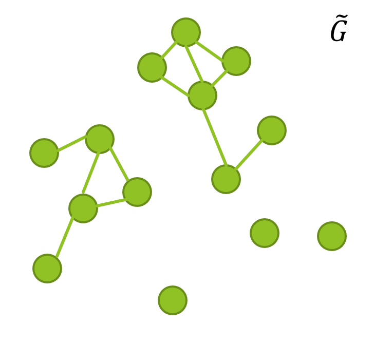
(a)

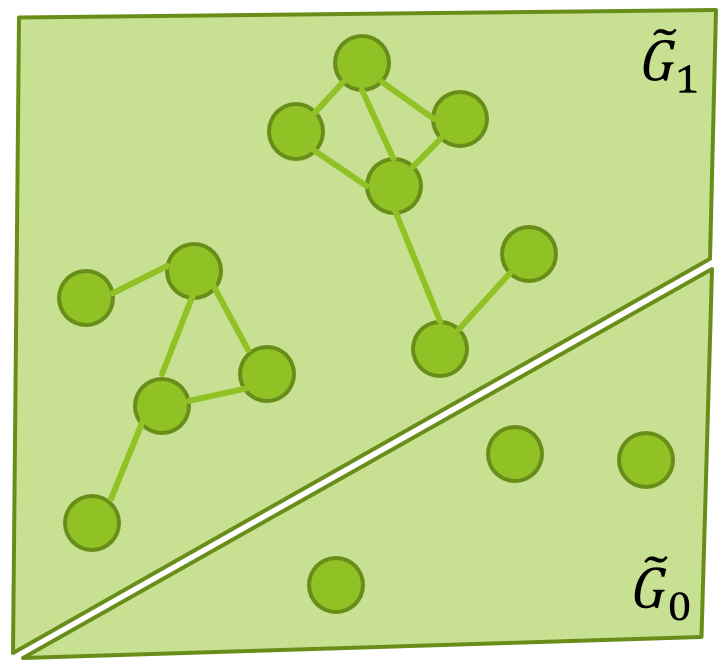
(b)

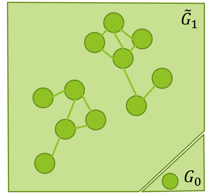
(c)

Figure 1: Schematic depiction of the construction of a DRIG. (a) First, a RIG is constructed, which will usually be oversized. (b) Next, this RIG is decomposed into the subgraph of isolated vertices and the remaining subgraph. (c) Finally, the subgraph of isolated vertices is removed and replaced by a graph of isolated vertices of specified size, which will usually be smaller.

We will denote a RIG by $G^{\mathrm{RIG}}(n^{\mathrm{RIG}},\beta,\gamma)$; it is of size $n^{\mathrm{RIG}}\in\mathbb{N}_{+}$ and has parameters $\beta,\gamma>0$. It has a set of enumerable vertices, e.g. $\mathcal{V}^{\mathrm{RIG}}=\{1,\ldots,n^{\mathrm{RIG}}\}$, and we also associate a set of enumerable attributes $\mathcal{A}^{\mathrm{RIG}}=\{1,\ldots,\lfloor\beta n^{\mathrm{RIG}}\rfloor\}$ to it. To construct the RIG, randomly connect every vertex $u\in\mathcal{V}^{\mathrm{RIG}}$ to each of the individual attributes $a\in\mathcal{A}^{\mathrm{RIG}}$ independently and with probability $\gamma/n^{\mathrm{RIG}}$. For $u\in\mathcal{V}^{\mathrm{RIG}}$, let $\mathcal{A}_{v}\subseteq\mathcal{A}$ be the set of attributes connected to vertex $u$. We now define the edge set of the RIG as $\mathcal{E}^{\mathrm{RIG}}=\{(u,v)\mid\mathcal{A}_{u}\cap\mathcal{A}_{v}\neq\varnothing\}$, i.e., the set of pairs of vertices that have at least one attribute in common.

We will denote a DRIG by $G^{\mathrm{DRIG}}(n^{\mathrm{DRIG}},\beta,\gamma,c)$, to indicate that it is of size $n^{\mathrm{DRIG}}\in\mathbb{N}_{+}$ and has parameters $\beta,\gamma,c>0$. Given values for these parameters, we construct the DRIG as follows. First, set $n^{\mathrm{RIG}}=\sigma n^{\mathrm{DRIG}}$ where we introduce

$$\sigma=\frac{1-e^{-c}}{1-\xi_{0}},\quad\textnormal{and}\quad\xi_{0}=\exp{\bigl{(}-\beta\gamma(1-e^{-\gamma})\bigr{)}},$$ (8)

and then construct $G^{\mathrm{RIG}}(n^{\mathrm{RIG}},\beta,\gamma)$ as described above. Now decompose this RIG into the subgraph $G^{\mathrm{RIG}}_{0}$ that consists of all of its isolated vertices, and the subgraph $G^{\mathrm{RIG}}_{1+}$ that consists of all of its vertices that have at least one neighbor. We now essentially remove the former subgraph and replace it: set $G^{\mathrm{DRIG}}=G^{\mathrm{DRIG}}_{0}\cup G^{\mathrm{RIG}}_{1+}$, where $G^{\mathrm{DRIG}}_{0}$ is a graph consisting of $n_{0}^{\mathrm{DRIG}}=\lfloor e^{-c}n^{\mathrm{DRIG}}\rfloor$ isolated vertices.

The parameters of a DRIG can be chosen to match three major features of the RGG: (i) the mean number of neighbors of a vertex; (ii) the probability that a vertex is isolated; and (iii) the probability that a triangle occurs in the graph. For each of the four types of graphs that we have discussed so far, Table 1 gives the explicit expressions for each of these quantities. The ability to match feature (iii) is new compared to an earlier approach that uses an ERRG [20]. The DRIG therefore captures more structural information of a RGG than an ERRG.

	$\mathbb{E}[N_{v}]$	$\mathbb{P}[\{u,v\},\{v,w\},\{w,u\}\in\mathcal{E}]$	$\mathbb{P}[N_{v}=0]$
RGG	$c$	$2\int\limits_{0}^{1}xI_{1-\frac{x^{2}}{4}}\left(\frac{3}{2},\frac{1}{2}\right)dx$	${\mathrm{e}}^{-c}$
ERRG	$c$	$0$	${\mathrm{e}}^{-c}$
RIG	$\beta\gamma^{2}$	$(1+\beta\gamma)^{-1}$	$\xi_{0}$
DRIG	$\frac{1-e^{-c}}{1-\xi_{0}}\beta\gamma^{2}$	$(1+\beta\gamma)^{-1}$	${\mathrm{e}}^{-c}$

Table 1: Properties (i), (ii), and (iii) of a DRIG compared to the other types of random graphs in the limit of $N\rightarrow\infty$. Here, $u\neq v\neq w$, $N_{v}$ denotes the number of neighbors of a vertex $v$ chosen uniformly at random, and $I_{\cdot}(\cdot,\cdot)$ the normalized incomplete beta integral.

III Results

III.1 Time-dependent evolution of the for a DRIG relevant quantities when conducting RSA on a RIG

We now analyze the time-dependent behavior of a graph exploration algorithm that iteratively simultaneously constructs a mixture of a RIG and a graph consisting solely of isolated vertices, as well as conduct RSA on this graph. The RSA process mimics the excitation process that happens within (a classical counterpart to) the QMMRG. This idea of using a graph exploration algorithm to describe the excitation process in a Rydberg gas was first described in [20], and here we first generalize the approach for application to a mixture of a RIG and a graph consisting solely of isolated vertices, and second lift the results through a time-transformation for application to a DRIG.

III.1.1 Graph exploration algorithm

Suppose that parameters $n^{\mathrm{DRIG}}\in\mathbb{N}_{+}$, $\beta,\gamma,c>0$ are fixed and given. The algorithm will give each vertex one of the labels ‘unaffected, excited, blocked’ iteratively as follows:

Initialization. First, we label all vertices as being unaffected. The initial number of unaffected vertices in $G^{\mathrm{RIG}}=G_{0}^{\mathrm{RIG}}\cup G_{1+}^{\mathrm{RIG}}$ and $G^{\mathrm{DRIG}}_{0}$ are therefore

$$U^{\mathrm{RIG}}(0)=n^{\mathrm{RIG}},\enskip U_{0}^{\mathrm{DRIG}}(0)=\lfloor{\mathrm{e}}^{-c}n^{\mathrm{DRIG}}\rfloor$$ (9)

say, respectively. The initial number of excited vertices in $G_{1+}^{\mathrm{RIG}}$ and $G_{0}^{\mathrm{DRIG}}$ are

$$X_{1+}^{\mathrm{RIG}}(0)=X_{0}^{\mathrm{DRIG}}(0)=0$$ (10)

say, respectively. We will define $n=n^{\mathrm{RIG}}+\lfloor{\mathrm{e}}^{-c}n^{\mathrm{DRIG}}\rfloor$ here for notational convenience, which is the total number of vertices in the mixture of the RIG and the graph consisting solely of isolated vertices that we are about to explore.

Exploration. Consider now iteration $t\in\mathbb{N}_{+}$. For the $t$-th step of the exploration algorithm, select if possible a vertex $V(t)$ uniformly at random from the set of unaffected vertices, which has size

$$U^{\mathrm{RIG}}(t-1)+U_{0}^{\mathrm{DRIG}}(t-1).$$ (11)

Adjust the label of this vertex to excited. Change any label of an unaffected neighbor of $V(t)$ into blocked.

Case 1: Consider now the event that the vertex $V(t)$ was picked from the graph $G^{\mathrm{RIG}}$. If this event occurs, then the number of unaffected vertices will have decreased by one plus its number of unaffected neighbors, i.e.,

$$U^{\mathrm{RIG}}(t)=U^{\mathrm{RIG}}(t-1)-1-N_{V(t)}(t-1),$$ (12)

where $N_{V(t)}(t-1)$ denotes the number of unaffected neighbors of $V(t)$ after iteration $t-1$. Furthermore,

$$U_{0}^{\mathrm{DRIG}}(t)=U_{0}^{\mathrm{DRIG}}(t-1).$$ (13)

The number of excited vertices within $G^{\mathrm{RIG}}_{1+}$ only increases by one if $V(t)$ originated from $G^{\mathrm{RIG}}_{1+}$. In other words,

$$X_{1+}^{\mathrm{RIG}}(t)=X_{1+}^{\mathrm{RIG}}(t-1)+\mathds{1}[N_{V(t)}(t-1)>0],$$

$$X_{0}^{\mathrm{DRIG}}(t)=X_{0}^{\mathrm{DRIG}}(t-1).$$ (14)

Conditional on the history $\mathcal{F}(t)$, the event that $V(t)$ originates from $G^{\mathrm{RIG}}$ occurs with probability

$$\frac{U^{\mathrm{RIG}}(t-1)}{U^{\mathrm{RIG}}(t-1)+U_{0}^{\mathrm{DRIG}}(t-1)}.$$ (15)

Case 2: Consider now the complementary event: viz., the event that the vertex $V(t)$ came from $G^{\mathrm{DRIG}}_{0}$. If this event occurs, then the number of unaffected vertices decreases by one since this particular vertex has no neighbors, i.e.,

$$U^{\mathrm{RIG}}(t)=U^{\mathrm{RIG}}(t-1),\enskip U_{0}^{\mathrm{DRIG}}(t)=U_{0}^{\mathrm{RIG}}(t)-1.$$ (16)

Moreover, the number of excited vertices increases by one, so

$$X_{1+}^{\mathrm{RIG}}(t)=X_{1+}^{\mathrm{RIG}}(t-1),\enskip X_{0}^{\mathrm{DRIG}}(t)=X_{0}^{\mathrm{DRIG}}(t-1)+1.$$ (17)

Conditional on the history $\mathcal{F}(t)$, this event occurs with probability

$$\frac{U_{0}^{\mathrm{DRIG}}(t-1)}{U^{\mathrm{RIG}}(t-1)+U_{0}^{\mathrm{DRIG}}(t-1)}$$ (18)

For the graph exploration algorithm just described, we are able to prove results on its jamming limit and its fluid limit.

III.1.2 Jamming limit

Define for $t\in\mathbb{N}_{0}$,

$$U(t)=U^{\mathrm{RIG}}(t)+U_{0}^{\mathrm{DRIG}}(t),\quad\textnormal{and}$$ (19)

$$X(t)=X_{0}^{\mathrm{RIG}}(t)+X_{1+}^{\mathrm{RIG}}(t)+X_{0}^{\mathrm{DRIG}}(t).$$ (20)

Consider now

$$T^{*}=\min\{t\in\{0,1,\ldots,n\}\mid U(t)=0\},$$ (21)

the hitting time of zero of the stochastic process $\{U(t)\}_{0\leq t\leq n}$. Note that $T^{*}$ is a random variable and in particular that $T^{*}$ equals the number of excited vertices in the jamming limit. Leveraging this insight, we are able to prove convergence in probability of the fraction of excited vertices in the jamming limit to an implicitly characterized constant $\phi$ by conducting a hitting time analysis in Appendix A:

Theorem 1.

Let $T_{n}^{*}=T^{*}/n$. For any $\gamma>0$,

$$\mathbb{P}[|T_{n}^{*}-\phi|\geq\gamma]\to 0$$ (22)

as $n\to\infty$. Here,

$$0\leq\phi=\frac{e^{-c}+\sigma\arg\inf\bigl{\{}0\leq s\leq 1:\tilde{u}(s)=0\bigr{\}}}{e^{-c}+\sigma}\leq 1$$ (23)

where $\tilde{u}$ satisfies the following system of integral equations: for $0\leq s\leq 1$,

$$\tilde{u}(s) =1-s-\int_{0}^{s}\gamma^{2}\tilde{u}(y)\tilde{w}(y)\operatorname{d}\!{y},$$

$$\tilde{w}(s) =\beta-\int_{0}^{s}\gamma\tilde{w}(y)\operatorname{d}\!{y}.$$ (24)

Note that Theorem 1 establishes that in this mixture of a RIG and a graph consisting solely of isolated vertices, the final number of excited vertices satisfies

$$X(n)\approx\phi n.$$ (25)

Theorem 1 implies also that in a DRIG, the final number of excited vertices

$$X^{\mathrm{DRIG}}(n^{\mathrm{DRIG}})=X(n)-X_{0}^{\mathrm{RIG}}(n)$$

$$\approx\phi n-\sigma\xi_{0}n^{\mathrm{DRIG}}=(\phi(\sigma+{\mathrm{e}}^{-c})-\sigma\xi_{0})n^{\mathrm{DRIG}}=\eta n^{\mathrm{DRIG}}$$ (26)

say. Moreover, (23) together with (24) gives an implicit closed-form expression for $\phi$ and $\eta$.

III.1.3 Fluid limits

In fact, we are able to prove stronger fluid limits for the stochastic processes $\{U(t)\}_{0\leq t\leq n}$, $\{X(t)\}_{0\leq t\leq n}$ in Theorem 2. Its proof is relegated to Appendix B. Fluid limits are functional laws of large numbers, and describe the function to which (an appropriately scaled variant of) the process converges to leading order. An example of the convergence of the RSA process is shown in Figure 2. We require these fluid limits to ultimately describe the time-dependent behavior of the RSA process on a DRIG in Theorem 3.

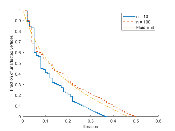
Figure 2: The unaffected number of vertices of the RSA process on the random graph for $n=10$ and $n=100$ vertices and the corresponding fluid limit $u(s)=u^{\mathrm{RIG}}(s)+u^{\mathrm{DRIG}}_{0}(s)$ in Theorem 2.

Theorem 2 (Fluid limits of $U(t),X(t)$ when conducting RSA on the mixture of a RIG and isolated vertices).

For any $0\leq S<\phi\leq 1$, $\varepsilon>0$,

$$\mathbb{P}\Bigl{[}\sup_{s\in[0,S]}\Bigl{|}\frac{U(\lfloor sn\rfloor)}{n}-(u^{\mathrm{RIG}}+u_{0}^{\mathrm{DRIG}})(s)\Bigr{|}>\varepsilon\Bigr{]}\to 0$$ (27)

as $n\to\infty$. Furthermore,

$$\mathbb{P}\Bigl{[}\sup_{s\in[0,S]}\Bigl{|}\frac{X(\lfloor sn\rfloor)}{n}-(x_{0}^{\mathrm{RIG}}+x_{1+}^{\mathrm{RIG}}+x_{0}^{\mathrm{DRIG}})(s)\Bigr{|}>\varepsilon\Bigr{]}\to 0$$ (28)

as $n\to\infty$. Here, the functions $u^{\mathrm{RIG}}$, $u_{0}^{\mathrm{DRIG}}$, $x_{0}^{\mathrm{RIG}}$, $x_{1+}^{\mathrm{RIG}}$, and $x_{0}^{\mathrm{DRIG}}$ satisfy the following system of integral equations: for $0\leq s\leq S<\phi\leq 1$ and $\tilde{\gamma}=(\sigma+e^{-c})\gamma/\sigma$,

$$u^{\mathrm{RIG}}(s) =\frac{\sigma}{\sigma+e^{-c}}-\int\limits_{0}^{s}\frac{u^{\mathrm{RIG}}(y)}{u^{\mathrm{RIG}}(y)+u_{0}^{\mathrm{DRIG}}(y)}\bigl{(}1+\tilde{\gamma}^{2}u^{\mathrm{RIG}}(y)w(y)\bigr{)}\operatorname{d}\!{y},$$ (29)

$$u_{0}^{\mathrm{DRIG}}(s) =\frac{e^{-c}}{\sigma+e^{-c}}-\int\limits_{0}^{s}\frac{u_{0}^{\mathrm{DRIG}}(y)}{u^{\mathrm{RIG}}(y)+u_{0}^{\mathrm{DRIG}}(y)}\operatorname{d}\!{y},$$ (30)

$$w^{\mathrm{RIG}}(s) =\frac{\beta\sigma}{\sigma+e^{-c}}-\int\limits_{0}^{s}\frac{u^{\mathrm{RIG}}(y)}{u^{\mathrm{RIG}}(y)+u_{0}^{\mathrm{DRIG}}(y)}\tilde{\gamma}w^{\mathrm{RIG}}(y)\operatorname{d}\!{y},$$ (31)

$$x_{0}^{\mathrm{RIG}}(s) =\int\limits_{0}^{s}\frac{u^{\mathrm{RIG}}(y)}{u^{\mathrm{RIG}}(y)+u_{0}^{\mathrm{DRIG}}(y)}\exp{\Bigl{(}-\tilde{\gamma}w^{\mathrm{RIG}}(y)\bigl{(}1-e^{-\tilde{\gamma}(\frac{\sigma}{\sigma+e^{-c}}-x_{0}^{\mathrm{RIG}}(y)-x_{1+}^{\mathrm{RIG}}(y))}\bigr{)}\Bigr{)}}\operatorname{d}\!{y},$$ (32)

$$x_{1+}^{\mathrm{RIG}}(s) =\int\limits_{0}^{s}\frac{u^{\mathrm{RIG}}(y)}{u^{\mathrm{RIG}}(y)+u_{0}^{\mathrm{DRIG}}(y)}\Bigl{(}1-\exp{\Bigl{(}-\tilde{\gamma}w^{\mathrm{RIG}}(y)\bigl{(}1-e^{-\tilde{\gamma}(\frac{\sigma}{\sigma+e^{-c}}-x_{0}^{\mathrm{RIG}}(y)-x_{1+}^{\mathrm{RIG}}(y))}\bigr{)}\Bigr{)}}\Bigr{)}\operatorname{d}\!{y},$$ (33)

$$x_{0}^{\mathrm{DRIG}}(s) =\int\limits_{0}^{s}\frac{u_{0}^{\mathrm{DRIG}}(y)}{u^{\mathrm{RIG}}(y)+u_{0}^{\mathrm{DRIG}}(y)}\operatorname{d}\!{y}.$$ (34)

III.2 Time-dependent evolution of the fraction of excited vertices when conducting RSA on a DRIG

The time-evolution of $U(t)$ for $t\in\{0,1,\ldots,n\}$ does not describe the number of unaffected vertices when conducting RSA on a DRIG, $D(t)$ for $t\in\{0,1,\ldots,n^{\mathrm{DRIG}}\}$ say. Recall for instance that $n=n^{\mathrm{RIG}}+\lfloor{\mathrm{e}}^{-c}n^{\mathrm{DRIG}}\rfloor$, which not necessarily equals $n^{\mathrm{DRIG}}$; the graph we are exploring is bigger. To obtain $D(t)$ one can utilize the graph exploration algorithm of Section III.1.1, but must then (i) filter out the vertices from $G^{\mathrm{RIG}}_{0}$, which are by definition not part of the DRIG, and (ii) afterwards apply an appropriate nonlinear time transformation. The latter must be done carefully and is nontrivial because early in the graph exploration, relatively more vertices may have come from $G^{\mathrm{RIG}}_{1+}$. The issue of overcounting and rescaling of iteration time is also illustrated using an example sample path in Table 2.

Sequence	Sample	Remark
$\{U(t-1)-U(t)\}_{t=1,\ldots,n}$	$2,1,2,3,1,5,1,4,2,1,1,1,3,4,1,6,2,1,\ldots,0,0,0,\ldots,0$	Decrements describing the number of unaffected vertices in the RIG. Identically zero after the random hitting time $T_{n}$.
$\{\mathds{1}[V(t)\in\mathcal{V}(G_{1+}^{\mathrm{RIG}})]\}_{t=1,\ldots,n}$	$1,1,1,1,0,1,0,1,1,1,0,1,1,1,0,1,1,1,\ldots,0,0,0,\ldots,0$	Steps at which a vertex was activated from $G_{1+}^{\mathrm{RIG}}$. These vertices are in the DRIG.
$\{\mathds{1}[V(t)\in\mathcal{V}(G_{0}^{\mathrm{DRIG}})]\}_{t=1,\ldots,n}$	$0,0,0,0,1,0,0,0,0,0,1,0,0,0,0,0,0,0,\ldots,0,0,0,\ldots,0$	Steps at which a vertex was activated from $G_{0}^{\mathrm{DRIG}}$. These vertices are in the DRIG.
$\{\mathds{1}[V(t)\in\mathcal{V}(G_{0}^{\mathrm{RIG}})]\}_{t=1,\ldots,n}$	$0,0,0,0,0,0,1,0,0,0,0,0,0,0,1,0,0,0,\ldots,0,0,0,\ldots,0$	Steps at which a vertex was activated from $G_{0}^{\mathrm{RIG}}$. These vertices are not in the DRIG.
$\{D(t-1)-D(t)\}_{t=1,\ldots,n^{\mathrm{DRIG}}}$	$2,1,2,3,1,5,\phantom{1,}\,4,2,1,1,1,3,4,\phantom{1,}\,6,2,1,\ldots,0,0,0,\ldots,0$	Decrements describing the number of unaffected vertices in the DRIG. For sufficiently large $n$, this is a shorter sequence with high probability.

Table 2: A sample sequence of decrements that describes the number of unaffected vertices in the mixture of a RIG with isolated vertices. We show how from it, we can find a coupled sequence of decrements describing the number of unaffected vertices in a DRIG. This illustrates the issue of overcounting and necessity of transforming iteration time when going from a result for the mixture of the RIG with isolated vertices to a result for the DRIG.

Concretely, the filtering out of vertices can be done by setting for $t\in\{0,1,\ldots,n\}$,

$$U^{\mathrm{DRIG}}(t)=U_{0}^{\mathrm{DRIG}}(t)+U_{1+}^{\mathrm{DRIG}}(t)$$

$$=U_{0}^{\mathrm{DRIG}}(t)+U^{\mathrm{RIG}}(t)+X_{0}^{\mathrm{RIG}}(t)-X_{0}^{\mathrm{RIG}}(n).$$ (35)

Rescaling iteration time can then be done appropriately by levering the inverse process

$$(X^{\mathrm{DRIG}})^{\leftarrow}(u)=\inf{\bigl{\{}t\in\mathbb{N}_{0}\big{|}X_{0}^{\mathrm{DRIG}}(t)+X_{1+}^{\mathrm{RIG}}(t)=u\bigr{\}}}$$ (36)

for $u\in\{0,1,\ldots,n^{\mathrm{DRIG}}\}$ to only count those steps that involve excitations from the DRIG. That is, for $t\in\{0,1,\ldots,n^{\mathrm{DRIG}}\}$, we define

$$D^{\mathrm{DRIG}}(t)=U^{\mathrm{DRIG}}((X^{\mathrm{DRIG}})^{\leftarrow}(t)).$$ (37)

Fortunately, all fluid limits necessary for obtaining a fluid limit for (37) are provided by Theorem 2. We prove the following in Appendix C:

Theorem 3 (Fluid limit of $D(t)$ when conducting RSA on a DRIG).

For $0\leq S<\eta\leq 1$, $\varepsilon>0$,

$$\mathbb{P}\Bigl{[}\sup_{s\in[0,S]}\Bigl{|}\frac{D(\lfloor sn^{\mathrm{DRIG}}\rfloor)}{n^{\mathrm{DRIG}}}-d(s)\Bigr{|}\geq\varepsilon\Bigr{]}\to 0$$ (38)

as $n^{\mathrm{DRIG}}\to\infty$. Here, for $0\leq s\leq S<\eta\leq 1$,

$$d(s)=(\sigma+e^{-c})u^{\mathrm{DRIG}}\bigl{(}(x^{\mathrm{DRIG}})^{\leftarrow}((\sigma+e^{-c})^{-1}s)\bigr{)},$$ (39)

and

$$u^{\mathrm{DRIG}}(s) =(u^{\mathrm{RIG}}+u_{0}^{\mathrm{DRIG}}+x_{0}^{\mathrm{RIG}})(s)-\xi_{0},$$

$$x^{\mathrm{DRIG}}(s) =(x_{1+}^{\mathrm{RIG}}+x_{0}^{\mathrm{DRIG}})(s).$$

III.3 Translating from iteration steps to actual time

Finally, if one is interested in translating iteration steps (in the arb. unit) to actual time (in e.g. seconds), then one may proceed as follows. Assume that the time between two steps is exponentially distributed with parameter $\lambda D(m)>0\,[${\mathrm{s}}^{-1}$]$ and independent of the past. Viz., $T_{m+1}-T_{m}\sim\textnormal{Exp}(\lambda D(m))\,$\mathrm{s}$$ for all $m\in\mathbb{N}_{+}$. Define then for $t\geq 0\,[$\mathrm{s}$]$, the process $X^{\prime}(t)=X(\sup\{m\in\mathbb{N}_{0}\mid t\geq T_{m}\})$ whose domain is actual time in seconds. This process satisfies for all $t\geq 0\,[$\mathrm{s}$]$,

$$\frac{\mathbb{E}[X^{\prime}(t)]}{n^{\mathrm{DRIG}}}\,[\mathrm{arb.}]\to\int_{0}^{t}\lambda d(x(s))\operatorname{d}\!{s}\,[\mathrm{arb.}]$$ (40)

as $n^{\mathrm{DRIG}}\to\infty$. This was also discussed in [20].

IV Heuristics

In this section, we come up with a heuristic using random graphs that gives a recursion to describe the following normalized pair-correlation function

$$h_{\varepsilon}(r)=\frac{\mathbb{P}_{N}[v,w\in\hat{X}(\infty)\mid d(v,w)\in(r-\epsilon,r+\epsilon)]}{\mathbb{P}_{N}[v\in\hat{X}(\infty)]^{2}}$$ (41)

say, for a Rydberg gas. Here, $\hat{X}(\infty)$ denotes the set of excited vertices in the jamming limit. We chose this function for comparison purposes to [39, Fig. 2].

Many random graphs are however not built around an explicit notion of distance $d(v,w)$ between two vertices $v,w\in\mathcal{V}$, so evaluation of (41)’s numerator is impossible. Given a random graph without a notion of distance, such as an ERRG, we need to instead use a proxy for the distance between two vertices. Using such a proxy comes at a cost: the following approach is a heuristic, and we have no mathematical results guaranteeing its accuracy. Nonetheless, the approaches will turn out descriptive. As our proxy for a notion of distance, we will specifically use the number of neighbors that two vertices have in common. The idea is that if two vertices have more neighbors in common, then their distance should be smaller.

Heuristic 1 (Recursive system to approximate a normalized pair correlation function of a RGG or the QMMRG).

For all $v,w\in\mathcal{V}$, $r\in(0,2r_{b}]$, $0<\epsilon\ll 1$: the numerator in (41) satisfies

$$\mathbb{P}_{N}[v,w\in\hat{X}(\infty)\mid d(v,w)\in(r-\epsilon,r+\epsilon)] =\begin{cases}0&\textnormal{if }0<r<r_{b}\\ \displaystyle\sum_{i,k}A_{i,k}^{N}(r)B_{i,k}^{N}(r)C_{i}^{N}(r)\approx\displaystyle\sum_{i,k}\hat{A}_{i,k}^{N}(r)\hat{B}_{i,k}(r)\hat{C}_{i}^{N}&\textnormal{otherwise}\\ \end{cases}$$ (42)

Here,

$$A_{i,k}^{N}(r) =\mathbb{P}_{N}[v,w\in\hat{X}(\infty)\mid\lvert\hat{N}_{v}\cap\hat{N}_{w}\rvert=k,N_{v}=i,d(v,w)\in(r-\epsilon,r+\epsilon)],$$

$$B_{i,k}^{N}(r) =\mathbb{P}_{N}[\lvert\hat{N}_{v}\cap\hat{N}_{w}\rvert=k\mid N_{v}=i,d(v,w)\in(r-\epsilon,r+\epsilon)],$$

$$C_{i}^{N}(r) =\mathbb{P}_{N}[N_{v}=i\mid d(v,w)\in(r-\varepsilon,r+\varepsilon)],$$ (43)

and

$$A_{i,k}^{N}(r) \approx\hat{A}_{i,k}^{N}(r)$$

$$=\frac{1}{N}\hat{E}^{N-i-1}(r)+\frac{1}{N}\sum_{j=0}^{N-i-2}\binom{N-i-2}{j}\bigl{(}p(1-F_{1}(r))\bigr{)}^{j}\bigl{(}1-p(1-F_{1}(r))\bigr{)}^{N-i-2-j}\hat{D}_{i-k}^{N-k-j-1}$$ (44)

$$\phantom{=}+\frac{N-i-2}{N}\bigl{(}1-p(1-F_{1}(r))\bigr{)}$$

$$\phantom{=+}\times\sum_{j=0}^{N-i-3}\sum_{l=0}^{k}\sum_{m=0}^{i-k}\binom{N-i-3}{j}(pF_{2}(r))^{j}\bigl{(}1-pF_{2}(r)\bigr{)}^{N-i-3-j}\binom{k}{l}p^{l}(1-p)^{k-l}$$

$$\phantom{=\times\sum_{j=0}^{N-i-3}\sum_{l=0}^{k}\sum_{m=0}^{i-k}}\times\binom{i-k}{m}\bigl{(}p(1-F_{1}(r))\bigr{)}^{m}\bigl{(}1-p(1-F_{1}(r))\bigr{)}^{i-k-m}\hat{A}_{i-l-m,k-l}^{N-j-l-m-1}(r)$$ (45)

as well as

$$B_{i,k}^{N}(r)\approx\hat{B}_{i,k}(r)=\binom{i}{k}(F_{1}(r))^{k}\bigl{(}1-F_{1}(r)\bigr{)}^{i-k},$$ (46)

$$C_{i}^{N}(r)\approx\hat{C}_{i}^{N}=\binom{N-2}{i}p^{i}(1-p)^{N-2-i}.$$ (47)

Here, $p=c/N$,

$$\hat{D}_{i}^{N}(r) =\frac{1}{N}+\frac{N-i-1}{N}\sum_{k=0}^{N-i-2}\sum_{l=0}^{i}\binom{N-i-2}{k}p^{k}(1-p)^{N-i-2-k}$$

$$\phantom{=\frac{1}{N}+\frac{N-i-1}{N}\sum_{k=0}^{N-i-2}\sum_{l=0}^{i}}\times\binom{i}{l}\bigl{(}p(1-F_{1}(r))\bigr{)}^{l}\bigl{(}1-p(1-F_{1}(r))\bigr{)}^{i-l}\hat{D}_{i-l}^{N-k-l-1}(r)$$ (48)

$$\hat{E}^{N}(r) =\frac{1}{N}+\frac{N-1}{N}\bigl{(}1-p(1-F_{1}(r))\bigr{)}\sum_{k=0}^{N-2}\binom{n-2}{k}p^{k}(1-p)^{N-2-k}\hat{E}^{N-k-1}(r);$$ (49)

and finally $F_{1}(r)=\frac{1}{\pi}\bigl{(}2\arccos{\frac{r}{2r_{b}}}-\frac{r}{2r_{b}}\sqrt{4-(\frac{r}{r_{b}})^{2}}\bigr{)}$ and $F_{2}(r)=\frac{\textsc{AREA}(C_{1}\cap C_{2}\cap C_{3})}{\textsc{AREA}(C_{1})}$, where $C_{1}$, $C_{2}$ and $C_{3}$ are circles with radii $r_{b}$, the distance between $C_{1}$ and $C_{2}$ is $r$, the distance between $C_{1}$ and $C_{3}$ is $r_{b}$ and the distance between $C_{2}$ and $C_{3}$ is $r_{b}$ (see [40] for a closed-form expression).

To understand how Heuristic 1 is established, start by noting that the first equality in (42) follows from the law of total probability and is still exact; essentially, we have partitioned the sample space according to the conditional events implicitly defined in (43). Next, we approximate each of these terms by relating them to a mathematical expression obtained from a random graph. For each term we use a random graph for which we believe the exploration process behaves similar to a classical counterpart of the excitation process of a QMMRG.

1. For the terms $A_{i,k}^{N}(r)$ and $C_{i}^{N}(r)$, we use what would be their explicit recursions in a random graph with one geometric feature and four classes of distances, that is, the expressions for $\hat{A}_{i,k}(r)$ and $\hat{C}_{i}^{N}$ in (44) and (47). Concretely, in this random graph:

• none of the vertices have an explicit position;

• vertices $v$ and $w$ are considered to be at exactly a distance $r$ of each other;

• all other vertices are either

  • – within a distance $r_{b}$ of $v$ but not $w$; or

  • – within a distance $r_{b}$ of $w$ but not $v$; or

  • – within a distance $r_{b}$ of both $v,w$; or

  • – outside of a distance $r_{b}$ of both $v,w$.

Depending on which class a vertex belongs to, the vertex’s probability of creating an edge with vertices of its own class and of other classes changes. For example (ignoring the precise conditioning for a moment), once $w$ is explored before $v$, then from that point onward, class 1 vertices will connect to $v$ with reduced probability $p(1-F_{1}(r))$ instead of the originally higher probability $p$. Here, the function $F_{1}(r)$ describes the fraction of surface area of one circle of radius $r_{b}$ that overlaps with the surface area of a second circle also of radius $r_{b}$ and that is a distance $r$ away from the first circle. As a consequence, $r$ can be at most $2r_{b}$ for the heuristic to work, otherwise the surface areas of the two circles would not overlap. A similar argument is used for all other cases, and for each case a suitable edge probability is chosen. It must be noted that these choices do not correspond exactly to the edge probabilities in e.g. a RGG—this is in fact impossible because there is almost no geometry in the present random graph—and are chosen instead for them being reasonable proxies (usually, they are upper bounds). The recursions are then found by conditioning on the first excitation.

2. For the term $B_{i,k}^{N}(r)$ we use what would be its explicit expressions in a RGG, viz., the expression $\hat{B}_{i,k}(r)$ in (46).

The resulting formula in Heuristic 1 is not particularly attractive. However, the right-hand side of (42) combined with the expressions in (43)–(48) do constitute a recursive system of expressions that can be evaluated. In particular, have a look at Figure 5 in Section V.2 as well as the surrounding discussion.

V Numerics

V.1 Comparison: RSA on (a DRIG vs an ERRG)

For a range of atomic densities, Figure 3 shows the relative difference between the ultimate mean number of excited atoms as predicted by: 1. RSA on an ERRG, 2. RSA on a DRIG, and 3. RSA on a RGG. Note that a closed-form expression is available in literature for this number in model 1 [20]; that we have derived an implicit expression for this number in model 2 in Theorem 1 in this paper; and that no analytical expression is available in literature for this number in model 3. Hence, the results for model 3 displayed here were obtained via numerical simulation only. Observe that the predictive power of model 2 for model 3 is improved across a wider range of atomic densities when compared to the predictive power of model 1 for model 3. Since model 3 mimics the excitation process in the QMMRG, we conclude that a RSA process on a DRIG allows for more accurate prediction of the statistics of the excitation dynamics in a Rydberg gas, than what was achieved by RSA on an ERRG [20]. From the mathematical perspective, it is also noteworthy that this observation indicates that the graph structure of a DRIG matches the graph structure of a RGG better.

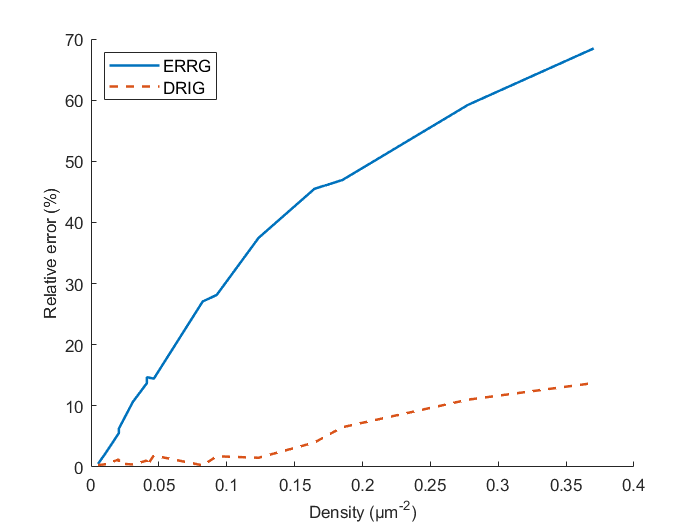
Figure 3: The relative difference between the mean ultimate number of excited atoms as predicted by RSA on an ERRG, a DRIG, and a RGG; as a function of atomic density.

V.2 Comparison:
QMMRG vs RSA on a (RGG vs DRIG)

For two different atomic densities, Figure 4 shows the mean number of excited atoms as a function of time as predicted by: A. the QMMRG, B. RSA on a RGG, and C. RSA on a DRIG. These curves were obtained numerically for models A and B through simulation, while for model C we implemented Theorem 3. Recall that, as discussed in Section II, these three models have been matched to each other using only a linear model for the blockade radius; $r_{b}=\alpha+(C_{6}/\Omega)^{1/6}$. Observe from Figure 5 that the Rydberg blockade is clearly at play in each model, since ultimately only a fraction of atoms reaches the excited level. The stable period that is entered after approximately $2.5\text{\,}\mathrm{\SIUnitSymbolMicro s}$ indicates the jamming limit. Note that in the jamming limit, the prediction by each model is near identical. Prior to the jamming limit, the mean number of excited atoms as predicted by models B, C also follows the mean number of excited atoms as predicted by model A roughly; the key difference are the observed quantum oscillations. We can imagine from an experimental viewpoint that if there is a large level of uncertainty in the timestamps of measurements compared to the period of these quantum oscillations, then the measurement curve will resemble the prediction of models B, C. The difference between the predictions of models A and B was 10% on average in all numerical experiments performed. The difference between the predictions of models A and C was 12% on average.

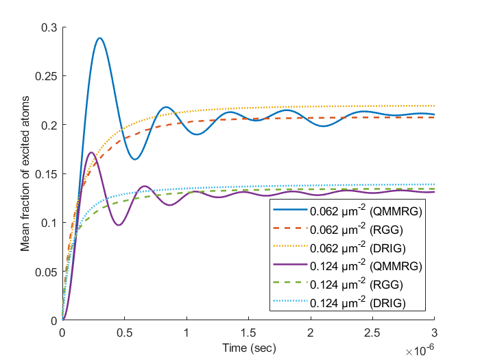
Figure 4: The mean fraction of atoms in their excited level for typical values of $\Omega=$5.8\text{\,}\mathrm{MHz}$$, $C_{6}=$50\text{\,}\mathrm{G}\mathrm{Hz}\mathrm{\SIUnitSymbolMicro}\mathrm{m}^{6}$$ as a function of time, and for two atomic densities, for models A, B and C. These curves were obtained numerically for models A and B through simulation, while for model C we implemented Theorem 3.

Figure 5 compares a normalized pair correlation function when measured in the jamming limit of: A. the QMMRG, B. a RSA process on a RGG, and D. our heuristic of Section IV. Here, we have temporarily replaced the hard blockade radius in model B specifically with a range-dependent blockade probability that takes the shape $p(r)=1/(1+\exp{(k(r-r_{b})))}$. Also, the linear model for the blockade radius has not been used here since we are interested in spatial correlations. Observe that the normalized pair correlation functions are quite similar: the random graph approaches are able to predict the normalized pair-correlation of the quantum mechanical model accurately over the displayed domain. Hence, Figure 5 also implies that the eventual spatial ordering of excited atoms resulting from either model A or B are similar. The displayed normalized pair-correlation function’s shape here is also roughly the same as in e.g. [39, Fig. 2]; as it should be.

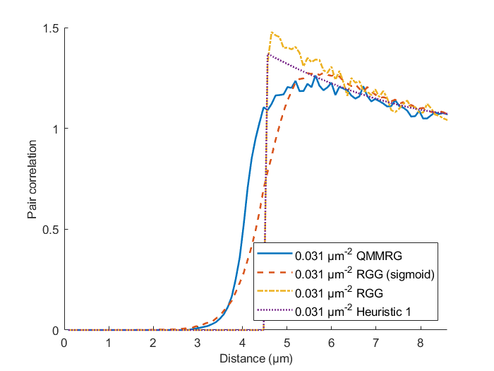
Figure 5: A normalized pair correlation function in the jamming limit for the QMMRG as compared to the RGG and Heuristic 1. Here, the density $\rho=$0.031\text{\,}\mathrm{\SIUnitSymbolMicro}\mathrm{m}^{-2}$$.

One remaining, open question raised by Figure 5 is whether these findings generalize to higher atomic densities. Our goal here was namely to simulate the quantum behavior as accurately as possible, and we forbade ourselves from applying advanced techniques to tackle the numerical complexities inherent in solving the Schrödinger equation. This meant that the number of simulated atoms was limited by our computer memory. Another open question is how these results compare to experimental measurements. A quick comparison of our results to e.g. the measured pair-correlation function in [41, Fig. 3] is unfortunately inconclusive. Firstly, the formula for the displayed pair-correlation function there in [41, (2)] differs from (41) which we display in Figure 5. In particular, their denominator is radius dependent, which ties in with this next point: their experimental setup differs from our model setups. The atoms were fixed in position using a square optical lattice instead of being distributed uniformly at random in two-dimensional space, and this affects the statistics.

VI Conclusion and Future work

We now revisit the question of the relative roles of geometrical restrictions induced by blockade effects and quantum mechanical effects, in the statistics of Rydberg gases. Our numerical comparison of the mean number of excitations over time shows that RSA processes on random graphs accurately predict the mean behavior of a quantum mechanical system over time but not the detailed oscillations induced by Schrödinger’s equation. We conclude that even without dissipation, on long time scales the statistics are affected most by the geometrical restrictions induced by blockade effects, while on short time scales the statistics are affected most by quantum effects. Our heuristic for describing a normalized pair correlation function shows that classical models can even predict the spatial statistics of Rydberg atoms to a considerable degree. We emphasize that no experimental averaging is taking place here: geometrical restrictions are the primary cause. The better mathematical tractability of classical models is an added boon.

If we take a wider viewpoint, we believe that incorporating geometrical restrictions into classical stochastic processes on simpler random graph models may allow for quantitative descriptions of also other statistical phenomena in strongly interacting, ultracold Rydberg gases. For example, Rydberg aggregates are networks of Rydberg atoms $\boldsymbol{X}^{[1]},\ldots,\boldsymbol{X}^{[n]}$ that define a region $S^{[n]}\subseteq\mathbb{R}^{3}$ that can nucleate, grow, and eventually reach a long-lived metastable arrangement when the atoms are off-resonantly excited [42]. The off-resonant excitation specifically causes that new Rydberg atoms shift the energy levels of atoms at a specific distance into resonance, and as a consequence after the nucleation of one Rydberg atom, regular arrangements of Rydberg atoms start to grow. We can model the growth mathematically by allowing only particles on the perimeter to become Rydberg atoms: $\boldsymbol{X}^{[n+1]}\sim\mathrm{Unif}(\partial S^{[n]})$. The stochastic recursions for this growth process will then be reminiscent of those in Section III and Appendix B but more complex due to $S^{[n]}$’s shape and the correlations between $\boldsymbol{X}^{[1]},\boldsymbol{X}^{[2]}$, etc. We anticipate that the mathematical framework of exploration processes on random graphs may suitably be adapted to quantitatively describe the growth of Rydberg aggregates.

Appendix A Proof of Theorem 1

The proof of Theorem 1 follows from two observations. First, the jamming limit $T^{*}$ equals the total time needed by an exploration process on a RIG of the random adsorption type plus an exploration process on a graph with isolated vertices. Second, establishing a fluid limit for the former exploration process can be done with a proof almost identical to the proof of Theorem 2, which is given in Appendix B. The only difference is that the argumentation of Appendix B.4 simplifies: the resulting fluid limit is namely Lipschitz continuous. Having established a fluid limit result for the exploration process on a RIG of the random adsorption type—for any $0\leq S\leq 1,\varepsilon>0$,

$$\mathbb{P}\Bigl{[}\sup_{s\in[0,S]}\Bigl{|}\frac{\tilde{U}^{\mathrm{RIG}}(\lfloor sn^{\mathrm{RIG}}\rfloor)}{n^{\mathrm{RIG}}}-\tilde{u}(s)\Bigr{|}>\varepsilon\Bigr{]}\to 0$$ (50)

as $n\to\infty$ say—one then proceeds as follows. Fix $\varepsilon>0,S\in[0,1]$ and suppose that at $t=\lfloor Sn^{\mathrm{RIG}}\rfloor$, $\tilde{U}(\lfloor Sn^{\mathrm{RIG}}\rfloor)\geq n^{\mathrm{RIG}}\varepsilon\geq 1$ for otherwise $\tilde{T}^{*}<\lfloor Sn^{\mathrm{RIG}}\rfloor$. Regardless, this implies that at $t=\lfloor Sn^{\mathrm{RIG}}+1\rfloor$, the hitting time $\tilde{T}^{*}$ satisfies the bound

$$(\lfloor Sn^{\mathrm{RIG}}\rfloor+1)\mathds{1}[n^{\mathrm{RIG}}\varepsilon\geq 1]\leq\tilde{T}^{*}\leq\lfloor Sn^{\mathrm{RIG}}\rfloor+\tilde{U}^{\mathrm{RIG}}(\lfloor Sn^{\mathrm{RIG}}\rfloor)\mathds{1}[n^{\mathrm{RIG}}\varepsilon\geq 1]\quad\textnormal{w.p.\ one}.$$ (51)

This is because either the exploration process finishes immediately in the next step (represented by the left-hand side), or finishes in at most $\tilde{U}(\lfloor Sn^{\mathrm{RIG}}\rfloor)$ more iteration steps (represented by the right-hand side). Note now that

$$\frac{\lfloor Sn^{\mathrm{RIG}}\rfloor}{n^{\mathrm{RIG}}}\mathds{1}[n^{\mathrm{RIG}}\varepsilon\geq 1]-\tilde{u}^{\leftarrow}(0)=\frac{\lfloor Sn^{\mathrm{RIG}}\rfloor}{n^{\mathrm{RIG}}}-\tilde{u}^{\leftarrow}(0)-\frac{\lfloor Sn^{\mathrm{RIG}}\rfloor}{n^{\mathrm{RIG}}}\mathds{1}[n^{\mathrm{RIG}}\varepsilon<1],$$ (52)

so that the scaled hitting time $\tilde{T}_{n^{\mathrm{RIG}}}^{*}=\tilde{T}^{*}/n^{\mathrm{RIG}}$ in particular satisfies the bound

$$\frac{\lfloor Sn^{\mathrm{RIG}}\rfloor}{n^{\mathrm{RIG}}}-\tilde{u}^{\leftarrow}(0)-\frac{\lfloor Sn^{\mathrm{RIG}}\rfloor}{n^{\mathrm{RIG}}}\mathds{1}[n^{\mathrm{RIG}}\varepsilon<1]+\frac{1}{n^{\mathrm{RIG}}}\mathds{1}[n^{\mathrm{RIG}}\varepsilon\geq 1]$$

$$\leq\tilde{T}_{n^{\mathrm{RIG}}}^{*}-\tilde{u}^{\leftarrow}(0)\leq\frac{\lfloor Sn^{\mathrm{RIG}}\rfloor}{n^{\mathrm{RIG}}}-\tilde{u}^{\leftarrow}(0)+\tilde{u}_{n^{\mathrm{RIG}}}(S)\mathds{1}[n^{\mathrm{RIG}}\varepsilon\geq 1],$$ (53)

w.p. one, and consequently

$$\frac{Sn^{\mathrm{RIG}}-1}{n^{\mathrm{RIG}}}-\tilde{u}^{\leftarrow}(0)-\mathds{1}[n^{\mathrm{RIG}}\varepsilon<1]\leq\tilde{T}_{n^{\mathrm{RIG}}}^{*}-\tilde{u}^{\leftarrow}(0)\leq\frac{Sn^{\mathrm{RIG}}}{n^{\mathrm{RIG}}}-\tilde{u}^{\leftarrow}(0)+\tilde{u}_{n^{\mathrm{RIG}}}(S)\quad\textnormal{w.p.\ one}.$$ (54)

We can now prove immediately that for any $\gamma>0$,

$$\lim_{n^{\mathrm{RIG}}\to\infty}\mathbb{P}[|\tilde{T}_{n^{\mathrm{RIG}}}^{*}-\tilde{u}^{\leftarrow}(0)|>\gamma]=0.$$ (55)

To see this, let $\gamma>0$. Bound the probability in (55) using (54), specify e.g. $\varepsilon<\gamma/2$ and $0<S=\tilde{u}^{\leftarrow}(\gamma/2)$, and finally take the limit (while utilizing (50)):

$$\mathbb{P}[|T_{n^{\mathrm{RIG}}}^{*}-\tilde{u}^{\leftarrow}(0)|>\gamma] \overset{\textnormal{(\ref{eqn:Intermediate_bound_for_hitting_time_RIG_only})}}{\leq}\mathbb{P}\Bigl{[}\frac{1}{n^{\mathrm{RIG}}}+\mathds{1}[n^{\mathrm{RIG}}\varepsilon<1]+\tilde{u}_{n^{\mathrm{RIG}}}(S)>\gamma\Bigr{]}$$

$$=\mathbb{P}\Bigl{[}\frac{1}{n^{\mathrm{RIG}}}+\mathds{1}[n^{\mathrm{RIG}}\varepsilon<1]+\tilde{u}(S)+\tilde{u}_{n^{\mathrm{RIG}}}(S)-\tilde{u}(S)>\gamma\Bigr{]}$$

$$\leq\mathbb{P}\Bigl{[}\frac{1}{n^{\mathrm{RIG}}}+\mathds{1}[n^{\mathrm{RIG}}\varepsilon<1]+\frac{\gamma}{2}+\varepsilon>\gamma\Bigr{]}+\mathbb{P}\Bigl{[}\sup_{s\in[0,S]}\Bigl{|}\frac{\tilde{U}(\lfloor sn^{\mathrm{RIG}}\rfloor)}{n^{\mathrm{RIG}}}-\tilde{u}(s)\Bigr{|}>\varepsilon\Bigr{]}\overset{\textnormal{(\ref{eqn:Fluid_limit_of_a_RIG_only})}}{\to}0$$ (56)

as $n^{\mathrm{RIG}}\to\infty$. This completes the proof.

Appendix B Proof of Theorem 2

Appendix B proves a fluid limit for the number of unaffected vertices in a mixture of a RIG and a graph consisting solely of isolated vertices. The idea here is to track both the number of unaffected vertices, as well as the number of unaffected attributes in the RIG and the number of unaffected vertices in an isolated graph. Their appropriately scaled counterparts can be decomposed in a drift part, which converges to a deterministic function; and a martingale part which vanishes as $n$ tends to infinity when scaled by $n$.

This method finds its roots in [20, 32, 33, 34, 35], but the approach differs here in that we study an exploration process on a subgraph of a mixture of two (random) graphs. This new approach requires us to determine a plethora of fluid limits, one for each of the relevant subgraphs of the mixture of (random) graphs, see Appendix B.4; and then combine these fluid limits using a nonlinear time transformation that depends on an inverse exploration process, see Appendix C. One further caveat is that because we mix two random graphs, a global Lipschitz’ continuity property of the fluid limit is lost. This therefore prevents application of the canonical approach of proving a fluid limit by utilizing global Lipschitz’ continuity prior to an application of Grönwell’s inequality. We circumvent this issue by conditioning only on sample paths that satisfy a local Lipschitz’ continuity, and subsequently showing that these sample paths occur with probability one in a large graph limit; see Appendix B.4.

Preliminaries

Recall that we are given parameters $n^{\mathrm{DRIG}}\in\mathbb{N}_{+}$, $\beta,\gamma,c>0$ according to which we conduct the graph exploration algorithm.

Definitions.

Let $G^{\mathrm{RIG}}=G_{0}^{\mathrm{RIG}}\cup G_{1+}^{\mathrm{RIG}}$ be a RIG with $n^{\mathrm{RIG}}=\lfloor(1-e^{-c})n^{\mathrm{DRIG}}/(1-\xi_{0})\rfloor$ vertices for $\xi_{0}=e^{-\beta\gamma(1-e^{-\gamma})}$ and parameters $m=\lfloor\beta n^{\mathrm{RIG}}\rfloor$ and $p=\gamma/n^{\mathrm{RIG}}$. Let $G_{0}^{\mathrm{DRIG}}$ be an isolated graph with $\lfloor{\mathrm{e}}^{-c}n^{\mathrm{DRIG}}\rfloor$ vertices. Define $n=n^{\mathrm{RIG}}+\lfloor{\mathrm{e}}^{-c}n^{\mathrm{DRIG}}\rfloor$ for convenience. For any vertex $v\in\mathcal{V}(G^{\mathrm{RIG}})\cup\mathcal{V}(G_{0}^{\mathrm{DRIG}})$, let $N_{v}$ be the set of neighbors of vertex $v$, i.e.,

$$\hat{N}_{v}=\begin{cases}\{w\in\mathcal{V}(G^{\mathrm{RIG}})\mid\hat{A}_{v}\cap\hat{A}_{w}\neq\emptyset,v\neq w\}&\text{if}\quad v\in\mathcal{V}(G^{\mathrm{RIG}}),\\ \emptyset&\text{if}\quad v\in\mathcal{V}(G_{0}^{\mathrm{DRIG}}).\end{cases}$$ (57)

Simultaneously with the RSA process, the DRIG and following objects will be iteratively constructed:

• Let $\hat{X}_{0}^{\mathrm{RIG}}(t)\subseteq\mathcal{V}(G_{0}^{\mathrm{RIG}})$ be the set of isolated, excited vertices at iteration $t$ from $G_{0}^{\mathrm{RIG}}$.

• Let $\hat{X}_{1+}^{\mathrm{RIG}}(t)\subseteq\mathcal{V}(G_{1+}^{\mathrm{RIG}})$ be the set of nonisolated, excited vertices at iteration $t$ from $G_{1+}^{\mathrm{RIG}}$.

• Let $\hat{X}_{0}^{\mathrm{DRIG}}(t)\subseteq\mathcal{V}(G_{0}^{\mathrm{DRIG}})$ be the set of excited vertices at iteration $t$ from $G_{0}^{\mathrm{DRIG}}$.

• Let $\hat{U}^{\mathrm{RIG}}(t)\subseteq\mathcal{V}(G^{\mathrm{RIG}})$ be the set of all unaffected vertices at iteration $t$ from $G^{\mathrm{RIG}}$. A vertex is unaffected if it is neither blocked nor excited.

• Let $\hat{U}_{0}^{\mathrm{DRIG}}(t)\subseteq\mathcal{V}(G_{0}^{\mathrm{DRIG}})$ be the set of unaffected vertices at iteration $t$ from $G_{0}^{\mathrm{DRIG}}$.

• Let $\hat{W}^{\mathrm{RIG}}(t)\subseteq\mathcal{A}$ be the set of all unaffected attributes at iteration $t$ from $G^{\mathrm{RIG}}$. An attribute is unaffected if no vertex connected to it has been excited.

Graph exploration algorithm.

Initially, at iteration $t=0$, set

$$\hat{X}_{0}^{\mathrm{RIG}}(0)=\emptyset,\enskip\hat{X}_{1+}^{\mathrm{RIG}}(t)(0)=\emptyset,\enskip\hat{X}_{0}^{\mathrm{DRIG}}(0)=\emptyset,\enskip\hat{U}^{\mathrm{RIG}}(0)=\mathcal{V}(G^{\mathrm{RIG}}),\enskip\hat{U}_{0}^{\mathrm{DRIG}}(0)=\mathcal{V}(G_{0}^{\mathrm{DRIG}}),\enskip\hat{W}^{\mathrm{RIG}}(0)=\mathcal{A}.$$ (58)

At each iteration $t\in\{1,2,\ldots,n\}$, a vertex $V(t)\in\hat{U}^{\mathrm{RIG}}(t-1)\cup\hat{U}_{0}^{\mathrm{DRIG}}(t-1)$ is selected uniformly at random from $\hat{U}^{\mathrm{RIG}}(t-1)\cup\hat{U}_{0}^{\mathrm{DRIG}}(t-1)$ as long as this set is nonempty. This vertex $V(t)$ is then labeled excited. Thus if $\hat{U}^{\mathrm{RIG}}(t-1)\cup\hat{U}_{0}^{\mathrm{DRIG}}(t-1)$ is nonempty, then the sets update:

$$\hat{X}_{0}^{\mathrm{RIG}}(t) =\begin{cases}\hat{X}_{0}^{\mathrm{RIG}}(t-1)\cup\{v\}&\textnormal{if }v\in\mathcal{V}(G^{\mathrm{RIG}}),\hat{N}_{v}=\emptyset,\\ \hat{X}_{0}^{\mathrm{RIG}}(t-1)&\text{otherwise},\end{cases}$$ (59)

$$\hat{X}_{1+}^{\mathrm{RIG}}(t) =\begin{cases}\hat{X}_{1+}^{\mathrm{RIG}}(t-1)\cup\{v\}&\textnormal{if }v\in\mathcal{V}(G^{\mathrm{RIG}}),\hat{N}_{v}\neq\emptyset,\\ \hat{X}_{1+}^{\mathrm{RIG}}(t-1)&\text{otherwise},\end{cases}$$ (60)

$$\hat{X}_{0}^{\mathrm{DRIG}}(t) =\begin{cases}\hat{X}_{0}^{\mathrm{DRIG}}(t-1)\cup\{v\}&\text{if }v\in\mathcal{V}(G_{0}^{\mathrm{DRIG}}),\\ \hat{X}_{0}^{\mathrm{DRIG}}(t-1)&\text{otherwise},\end{cases}$$ (61)

$$\hat{U}^{\mathrm{RIG}}(t) =\hat{U}^{\mathrm{RIG}}(t-1)\setminus(\{v\}\cup\hat{N}_{v}),$$ (62)

$$\hat{U}_{0}^{\mathrm{DRIG}}(t) =\hat{U}_{0}^{\mathrm{DRIG}}(t-1)\setminus\{v\},$$ (63)

$$\hat{W}^{\mathrm{RIG}}(t) =\hat{W}^{\mathrm{RIG}}(t-1)\setminus\hat{A}_{v}.$$ (64)

If otherwise $\hat{U}^{\mathrm{RIG}}(t-1)\cup\hat{U}_{0}^{\mathrm{DRIG}}(t-1)$ is empty, then the jamming limit has been reached and we set $\hat{X}_{0}^{\mathrm{RIG}}(t)=\hat{X}_{0}^{\mathrm{RIG}}(t-1)$, $\hat{X}_{1+}^{\mathrm{RIG}}(t)=\hat{X}_{0}^{\mathrm{RIG}}(t-1)$, et cetera, $\hat{W}^{\mathrm{RIG}}(t+1)=\hat{W}^{\mathrm{RIG}}(t)$.

B.1 The vector of set sizes constitutes a Markov chain

In this paper, we only need to investigate the stochastic evolution of the size of each set. We therefore define for $t\in\{0,1,\ldots,n\}$,

$$X_{0}^{\mathrm{RIG}}(t)=\lvert\hat{X}_{0}^{\mathrm{RIG}}(t)\rvert,\enskip X_{1+}^{\mathrm{RIG}}(t)=\lvert\hat{X}_{1+}^{\mathrm{RIG}}(t)\rvert,\enskip\textnormal{\emph{et cetera}},\enskip W^{\mathrm{RIG}}(t)=\lvert\hat{W}^{\mathrm{RIG}}(t)\rvert,$$ (65)

and for $t\in\{1,\ldots,n\}$,

$$X_{0}^{\mathrm{RIG}}(t)=X_{0}^{\mathrm{RIG}}(t-1)+\operatorname{d}\!{X_{0}^{\mathrm{RIG}}(t)},\enskip\textnormal{\emph{et cetera}},\enskip W^{\mathrm{RIG}}(t)=W^{\mathrm{RIG}}(t-1)+\operatorname{d}\!{W^{\mathrm{RIG}}(t)}.$$ (66)

Now: for $t\in\{0,1,\ldots,n\}$, consider the random vector

$$E(t)=\bigl{(}X_{0}^{\mathrm{RIG}}(t),X_{1+}^{\mathrm{RIG}}(t),X_{0}^{\mathrm{DRIG}}(t),U^{\mathrm{RIG}}(t),U_{0}^{\mathrm{DRIG}}(t),W^{\mathrm{RIG}}(t)\bigr{)},$$ (67)

for which we prove the following.

Lemma 1 (Markov chain and its drift).

The process $\{E(t)\}_{t\geq 0}$ is a Markov chain. Furthermore for $t\in\{1,\ldots,n\}$: if $U^{\mathrm{RIG}}(t-1)+U_{0}^{\mathrm{DRIG}}(t-1)\geq 1$, then

$$\mathbb{E}[E(t)| E(t-1)]-E(t-1)=$$

$$\Bigl{(}\phantom{-}\frac{U^{\mathrm{RIG}}(t-1)}{U^{\mathrm{RIG}}(t-1)+U_{0}^{\mathrm{DRIG}}(t-1)}\bigl{(}1-p+p(1-p)^{n^{\mathrm{RIG}}-X_{0}^{\mathrm{RIG}}(t-1)-X_{1+}^{\mathrm{RIG}}(t-1)}\bigr{)}^{W^{\mathrm{RIG}}(t-1)},$$ (68)

$$\phantom{-}\frac{U^{\mathrm{RIG}}(t-1)}{U^{\mathrm{RIG}}(t-1)+U_{0}^{\mathrm{DRIG}}(t-1)}\bigl{(}1-(1-p+p(1-p)^{n^{\mathrm{RIG}}-X_{0}^{\mathrm{RIG}}(t-1)-X_{1+}^{\mathrm{RIG}}(t-1)})^{W^{\mathrm{RIG}}(t-1)}\bigr{)},$$ (69)

$$\phantom{-}\frac{U_{0}^{\mathrm{DRIG}}(t-1)}{U^{\mathrm{RIG}}(t-1)+U_{0}^{\mathrm{DRIG}}(t-1)},$$ (70)

$$-\frac{U^{\mathrm{RIG}}(t-1)}{U^{\mathrm{RIG}}(t-1)+U_{0}^{\mathrm{DRIG}}(t-1)}(1+(U^{\mathrm{RIG}}(t-1)-1)(1-(1-p^{2})^{W^{\mathrm{RIG}}(t-1)})),$$ (71)

$$-\frac{U_{0}^{\mathrm{DRIG}}(t-1)}{U^{\mathrm{RIG}}(t-1)+U_{0}^{\mathrm{DRIG}}(t-1)},$$ (72)

$$-\frac{U^{\mathrm{RIG}}(t-1)}{U_{0}^{\mathrm{DRIG}}(t-1)+U^{\mathrm{RIG}}(t-1)}pW^{\mathrm{RIG}}(t-1)\Bigr{)};$$ (73)

otherwise, if $U^{\mathrm{RIG}}(t-1)+U_{0}^{\mathrm{DRIG}}(t-1)=0$, then $\mathbb{E}[E(t)|E(t-1)]=E(t-1)$ because a fortiori $E(t)=E(t-1)$.

Proof.

To prove that $\{E(t)\}_{t\geq 0}$ is a Markov chain, we need to show that for all trajectories $e(1),\ldots,e(t+1)$,

$$\mathbb{P}[E(t+1)=e(t+1)|E(1)=e(1),E(2)=e(2),\ldots,E(t)=e(t)]=\mathbb{P}[E(t+1)=e(t+1)|E(t)=e(t)].$$ (74)

We will split the task of showing (74) into examinations of the individual probability density functions describing the components of the vector $E(t)$. Let $\mathds{1}[\mathcal{E}]$ be the random variable that takes the value one if the event $\mathcal{E}$ is true, and zero otherwise. Substitute (64) into (66), and note that: if $U^{\mathrm{RIG}}(t)+U_{0}^{\mathrm{DRIG}}(t)>0$, then

$$\operatorname{d}\!{X_{0}^{\mathrm{RIG}}(t)} =\mathds{1}[V(t)\in\mathcal{V}(G^{\mathrm{RIG}})]\mathds{1}[N_{V(t)}=0],$$ (75)

$$\operatorname{d}\!{X_{1+}^{\mathrm{RIG}}(t)} =\mathds{1}[V(t)\in\mathcal{V}(G^{\mathrm{RIG}})](1-\mathds{1}[N_{V(t)}=0]),$$ (76)

$$\operatorname{d}\!{X_{0}^{\mathrm{DRIG}}(t)} =1-\mathds{1}[V(t)\in\mathcal{V}(G^{\mathrm{RIG}})],$$ (77)

$$\operatorname{d}\!{U^{\mathrm{RIG}}(t)} =-\mathds{1}[V(t)\in\mathcal{V}(G^{\mathrm{RIG}})](1+N_{V(t)}),$$ (78)

$$\operatorname{d}\!{U_{0}^{\mathrm{DRIG}}(t)} =-(1-\mathds{1}[V(t)\in\mathcal{V}(G^{\mathrm{RIG}})]),$$ (79)

$$\operatorname{d}\!{W^{\mathrm{RIG}}(t)} =-A_{V(t)}\mathds{1}[V(t)\in\mathcal{V}(G^{\mathrm{RIG}})];$$ (80)

otherwise $\operatorname{d}\!{X_{0}^{\mathrm{RIG}}(t)}=\cdots=\operatorname{d}\!{W^{\mathrm{RIG}}(t)}=0$. We now proceed component-wise.

Proof that $\operatorname{d}\!{X_{0}^{\mathrm{RIG}}(t)}|E(1),\ldots,E(t-1)\overset{\textnormal{(d)}}{=}\operatorname{d}\!{X_{0}^{\mathrm{RIG}}(t)}|E(t-1)$: First note that by construction,

$$\mathbb{P}[V(t)\in\mathcal{V}(G^{\mathrm{RIG}})|E(1),\ldots,E(t)]=\frac{U^{\mathrm{RIG}}(t-1)}{U^{\mathrm{RIG}}(t-1)+U_{0}^{\mathrm{DRIG}}(t-1)}\mathds{1}[U^{\mathrm{RIG}}(t-1)+U_{0}^{\mathrm{DRIG}}(t-1)\geq 1]$$ (81)

because $V(t)$ is selected uniformly at random from $\hat{U}_{0}^{\mathrm{DRIG}}(t-1)\cup\hat{U}^{\mathrm{RIG}}(t-1)$, independently. Note in particular that (81) also implies that $\mathbb{P}[V(t)\in\mathcal{V}(G^{\mathrm{RIG}})\mid E(1),\ldots,E(t)]=\mathbb{P}[V(t)\in\mathcal{V}(G^{\mathrm{RIG}})\mid E(t)]$—a fact that we will use later—but that this is not sufficient for proving the current claim.

To prove the current claim, note that $\operatorname{d}\!{X_{0}^{\mathrm{RIG}}(t)}\in\{0,1\}$. Therefore, using (80) and (i) the law of total probability, we find that

$$\mathbb{P}[\operatorname{d}\!{X_{0}^{\mathrm{RIG}}(t)}=1|E(1),\ldots,E(t-1)]$$

$$\overset{\textnormal{(\ref{eqn:Intermediate_expressions_for_dX_dU_dW_etc})}}{=}\mathbb{P}[V(t)\in\mathcal{V}(G^{\mathrm{RIG}}),N_{V(t)}=0|E(1),\ldots,E(t-1)]$$

$$\overset{\textnormal{(i)}}{=}\mathbb{P}[V(t)\in\mathcal{V}(G^{\mathrm{RIG}}),N_{V(t)}=0|E(1),\ldots,E(t-1),V(t)\in\mathcal{V}(G^{\mathrm{RIG}})]\mathbb{P}[V(t)\in\mathcal{V}(G^{\mathrm{RIG}})|E(1),\ldots,E(t-1)]$$

$$\phantom{=}+\mathbb{P}[V(t)\in\mathcal{V}(G^{\mathrm{RIG}}),N_{V(t)}=0|E(1),\ldots,E(t-1),V(t)\not\in\mathcal{V}(G^{\mathrm{RIG}})]\mathbb{P}[V(t)\not\in\mathcal{V}(G^{\mathrm{RIG}})|E(1),\ldots,E(t-1)]$$

$$=\mathbb{P}[V(t)\in\mathcal{V}(G^{\mathrm{RIG}})|E(1),\ldots,E(t-1)]\mathbb{P}[N_{V(t)}=0|E(1),\ldots,E(t-1),V(t)\in\mathcal{V}(G^{\mathrm{RIG}})].$$ (82)

Now by construction of the graph exploration algorithm, we have that

$$\mathbb{P}[N_{V(t)}=0|E(1),\ldots,E(t-1),V(t)\in\mathcal{V}(G^{\mathrm{RIG}})]$$

$$=\mathbb{E}\Bigl{[}(1-p)^{A_{V(t)}(n-X_{0}^{\mathrm{RIG}}(t-1)-X_{1+}^{\mathrm{RIG}}(t-1))}\Big{|}E(1),\ldots,E(t-1),V(t)\in\mathcal{V}(G^{\mathrm{RIG}})\Bigr{]}$$

$$=\bigl{(}1-p+p(1-p)^{n^{\mathrm{RIG}}-X_{0}^{\mathrm{RIG}}(t-1)-X_{1+}^{\mathrm{RIG}}(t-1)}\bigr{)}^{W^{\mathrm{RIG}}(t-1)}.$$ (83)

Substituting (81) and (83) into (82) implies that

$$\mathbb{P}[\operatorname{d}\!{X_{0}^{\mathrm{RIG}}(t)}=1|E(1),\ldots,E(t-1)]=\mathbb{P}[\operatorname{d}\!{X_{0}^{\mathrm{RIG}}(t)}=1|E(t-1)],$$ (84)

with the right-hand side here being equal to (68) because $\operatorname{d}\!{X_{0}^{\mathrm{RIG}}(t)}\in\{0,1\}$. Hence, this substitution also proves (68).

Proofs that $\operatorname{d}\!{X_{0}^{\mathrm{DRIG}}(t)}|E(1),\ldots,E(t-1)\overset{\textnormal{(d)}}{=}\operatorname{d}\!{X_{0}^{\mathrm{DRIG}}(t)}|E(t-1)$ and $\operatorname{d}\!{U_{0}^{\mathrm{DRIG}}(t)}|E(1),\ldots,E(t-1)\overset{\textnormal{(d)}}{=}\operatorname{d}\!{U_{0}^{\mathrm{DRIG}}(t)}|E(t-1)$: The first claim follows immediately from (81); see the discussion below it. Because $\operatorname{d}\!{X_{0}^{\mathrm{DRIG}}(t)}\in\{0,1\}$, (81) also implies (70). Combined with linearity, the exact same argumentation also proves the second claim as well as (72).

Proof that $\operatorname{d}\!{X_{1+}^{\mathrm{RIG}}(t)}|E(1),\ldots,E(t-1)\overset{\textnormal{(d)}}{=}\operatorname{d}\!{X_{1+}^{\mathrm{RIG}}(t)}|E(t-1)$: Combine the two previous arguments; linearity proves the current claim. On account of $\operatorname{d}\!{X_{1+}^{\mathrm{RIG}}(t)}\in\{0,1\}$, this approach also proves (69).

Proof that $\operatorname{d}\!{U^{\mathrm{RIG}}(t)}|E(1),\ldots,E(t-1)\overset{\textnormal{(d)}}{=}\operatorname{d}\!{U^{\mathrm{RIG}}(t)}|E(t-1)$: Let $k\in\mathbb{N}_{+}$. By (i) the law of total probability,

$$\mathbb{P}[\operatorname{d}\!{U^{\mathrm{RIG}}(t)}=-k|E(1),\ldots,E(t-1)]$$

$$\overset{\textnormal{(\ref{eqn:Intermediate_expressions_for_dX_dU_dW_etc})}}{=}\mathbb{P}[V(t)\in\mathcal{V}(G^{\mathrm{RIG}}),N_{V(t)}=k-1|E(1),\ldots,E(t-1)]$$

$$\overset{\textnormal{(i)}}{=}\mathbb{P}[V(t)\in\mathcal{V}(G^{\mathrm{RIG}}),N_{V(t)}=k-1|E(1),\ldots,E(t-1),V(t)\in\mathcal{V}(G^{\mathrm{RIG}})]\mathbb{P}[V(t)\in\mathcal{V}(G^{\mathrm{RIG}})|E(1),\ldots,E(t-1)]$$

$$\phantom{=}+\mathbb{P}[V(t)\in\mathcal{V}(G^{\mathrm{RIG}}),N_{V(t)}=k-1|E(1),\ldots,E(t-1),V(t)\not\in\mathcal{V}(G^{\mathrm{RIG}})]\mathbb{P}[V(t)\not\in\mathcal{V}(G^{\mathrm{RIG}})|E(1),\ldots,E(t-1)]$$

$$=\mathbb{P}[N_{V(t)}=k-1|E(1),\ldots,E(t-1),V(t)\in\mathcal{V}(G^{\mathrm{RIG}})]\mathbb{P}[V(t)\in\mathcal{V}(G^{\mathrm{RIG}})|E(1),\ldots,E(t-1)].$$ (85)

Note now that by construction, for $v\in\hat{U}^{\mathrm{RIG}}(t-1)$,

$$\mathbb{P}[N_{V(t)}=k-1|E(1),\ldots,E(t-1),V(t)\in\mathcal{V}(G^{\mathrm{RIG}}),V(t)=v]$$

$$=\sum_{a=0}^{W^{\mathrm{RIG}}(t-1)}\mathbb{P}[N_{V(t)}=k-1|E(1),\ldots,E(t-1),V(t)=v,|A_{v}|=a]\mathbb{P}[|A_{v}|=a|E(1),\ldots,E(t-1),v\in\mathcal{V}(G^{\mathrm{RIG}})]$$

$$=\sum_{a=0}^{W^{\mathrm{RIG}}(t-1)}\binom{U^{\mathrm{RIG}}(t-1)-1}{k-1}(1-(1-p)^{a})^{k-1}(1-p)^{a(U^{\mathrm{RIG}}(t-1)-k)}\binom{W^{\mathrm{RIG}}(t-1)}{a}p^{a}(1-p)^{W^{\mathrm{RIG}}(t-1)-a}.$$ (86)

Substituting (81) and (86) into (85), we find that for all $k\in\mathbb{N}_{+}$,

$$\mathbb{P}[\operatorname{d}\!{U^{\mathrm{RIG}}(t)}=k|E(1),\ldots,E(t-1)]=\mathbb{P}[\operatorname{d}\!{U^{\mathrm{RIG}}(t)}=k|E(t-1)].$$ (87)

Here, the right-hand side is implicitly given by the expression that results after the substitution.

We now proceed and calculate the drift. By (i) symmetry, and (ii) after substitution of (86) and algebraic manipulation, we find that

$$\mathbb{E}[\operatorname{d}\!{U^{\mathrm{RIG}}(t)}|E(t-1)]$$

$$=-\frac{U^{\mathrm{RIG}}(t-1)}{U^{\mathrm{RIG}}(t-1)+U_{0}^{\mathrm{DRIG}}(t-1)}$$

$$\phantom{=}\times\sum_{k=1}^{U^{\mathrm{RIG}}(t-1)}k\sum_{v\in\hat{U}^{\mathrm{RIG}}(t-1)}\mathbb{P}[N_{V(t)}=k-1|E(1),\ldots,E(t-1),V(t)\in\mathcal{V}(G^{\mathrm{RIG}}),V(t)=v]$$

$$\overset{\textnormal{(i,ii)}}{=}-\frac{U^{\mathrm{RIG}}(t-1)}{U^{\mathrm{RIG}}(t-1)+U_{0}^{\mathrm{DRIG}}(t-1)}\bigl{(}1-\bigl{(}U^{\mathrm{RIG}}(t-1)-1\bigr{)}\bigl{(}1-(1-p^{2})^{W^{\mathrm{RIG}}(t-1)}\bigr{)}\bigr{)}.$$ (88)

This proves (71).

Proof that $\operatorname{d}\!{W^{\mathrm{RIG}}(t)}|E(1),\ldots,E(t-1)\overset{\textnormal{(d)}}{=}\operatorname{d}\!{W^{\mathrm{RIG}}(t)}|E(t-1)$: Let $k\in\mathbb{N}_{0}$. By (i) the law of total probability, and (ii) symmetry of the vertices $v\in\hat{U}^{\mathrm{RIG}}(t-1)$,

$$\mathbb{P}[\operatorname{d}\!{W^{\mathrm{RIG}}(t)}=-k|E(1),\ldots,E(t-1)]$$

$$\overset{\textnormal{(\ref{eqn:Intermediate_expressions_for_dX_dU_dW_etc})}}{=}\mathbb{P}[A_{V(t)}=k,V(t)\in\mathcal{V}(G^{\mathrm{RIG}})|E(1),\ldots,E(t-1)]$$

$$\overset{\textnormal{(i)}}{=}\sum_{v\in\hat{U}^{\mathrm{RIG}}(t-1)\cup\hat{U}_{0}^{\mathrm{DRIG}}(t-1)}\mathbb{P}[A_{V(t)}=k,V(t)\in\mathcal{V}(G^{\mathrm{RIG}})|E(1),\ldots,E(t-1),V(t)=v]\mathbb{P}[V(t)=v|E(1),\ldots,E(t-1)]$$

$$\overset{\textnormal{(ii)}}{=}\frac{U^{\mathrm{RIG}}(t-1)}{U^{\mathrm{RIG}}(t-1)+U_{0}^{\mathrm{DRIG}}(t-1)}\binom{W^{\mathrm{RIG}}(t-1)}{k}p^{k}(1-p)^{W^{\mathrm{RIG}}(t-1)-k}.$$ (89)

Consequently, for all $k\in\mathbb{N}_{0}$,

$$\mathbb{P}[\operatorname{d}\!{W^{\mathrm{RIG}}(t)}=-k,|E(1),\ldots,E(t-1)]=\mathbb{P}[\operatorname{d}\!{W^{\mathrm{RIG}}(t)}=-k|E(t-1)].$$ (90)

This proves the current claim.

Inspecting (89), we can conclude that

$$-\operatorname{d}\!{W^{\mathrm{RIG}}(t)}|E(t-1),V(t)\in\mathcal{V}(G^{\mathrm{RIG}})\overset{\textnormal{(d)}}{=}\mathrm{Binomial}(W^{\mathrm{RIG}}(t-1),p),\quad\textnormal{and}$$

$$-\operatorname{d}\!{W^{\mathrm{RIG}}(t)}|E(t-1),V(t)\not\in\mathcal{V}(G^{\mathrm{RIG}})\overset{\textnormal{(d)}}{=}0\textnormal{ w.p.\ one}.$$ (91)

These two observations imply (73), which concludes the proof. ∎

B.2 Martingale decompositions and integral representations of the elements of $X_{0}^{\mathrm{RIG}}(t),X_{1+}^{\mathrm{RIG}}(t),\ldots,W^{\mathrm{RIG}}(t)$

For $s\in[0,1]$, define scaled variants of the set sizes by

$$x_{0,n}^{\mathrm{RIG}}(s)=\frac{X_{0}^{\mathrm{RIG}}(\lfloor sn\rfloor)}{n},\enskip x_{1+,n}^{\mathrm{RIG}}(s)=\frac{X_{1+}^{\mathrm{RIG}}(\lfloor sn\rfloor)}{n},\enskip x_{0,n}^{\mathrm{DRIG}}(s)=\frac{X_{0}^{\mathrm{DRIG}}(\lfloor sn\rfloor)}{n},\enskip\textnormal{\emph{et cetera}},\enskip w_{n}^{\mathrm{RIG}}(s)=\frac{W^{\mathrm{RIG}}(\lfloor sn\rfloor)}{n}.$$ (92)

Integral representation of $X_{0}^{\mathrm{RIG}}(t)$. Using Doob–Meyer’s decomposition theorem [43] on e.g. $X_{0}^{\mathrm{RIG}}(t)$, we find the martingale decomposition

$$X_{0}^{\mathrm{RIG}}(t) =\sum\limits_{i=1}^{t}\operatorname{d}\!{X_{0}^{\mathrm{RIG}}(t)}$$ (93)

$$=M_{n}^{X_{0}^{\mathrm{RIG}}}(t)+\sum\limits_{i=1}^{t}\frac{U^{\mathrm{RIG}}(i-1)\mathds{1}[U^{\mathrm{RIG}}(i-1)+U_{0}^{\mathrm{DRIG}}(i-1)\geq 1]}{U^{\mathrm{RIG}}(i-1)+U_{0}^{\mathrm{DRIG}}(i-1)}$$

$$\phantom{=M_{n}^{X_{0}^{\mathrm{RIG}}}(t)+\sum\limits_{i=1}^{t}}\times\bigl{(}1-p+p(1-p)^{n^{\mathrm{RIG}}-X_{0}^{\mathrm{RIG}}(i-1)-X_{1+}^{\mathrm{RIG}}(i-1)}\bigr{)}^{W^{\mathrm{RIG}}(i-1)},$$

with $M_{n}^{X_{0}^{\mathrm{RIG}}}(t)$ a square-integrable martingale. To see why, note that

$$M_{n}^{X_{0}^{\mathrm{RIG}}}(t)=\sum_{i=1}^{t}\bigl{(}X_{0}^{\mathrm{RIG}}(i)-X_{0}^{\mathrm{RIG}}(i-1)-\mathbb{E}[\operatorname{d}\!{X_{0}^{\mathrm{RIG}}(i)}|Z_{i-1}]\bigr{)}=\sum_{i=1}^{t}\bigl{(}\operatorname{d}\!{X_{0}^{\mathrm{RIG}}(i)}-\mathbb{E}[\operatorname{d}\!{X_{0}^{\mathrm{RIG}}(i)}|Z_{i-1}]\bigr{)}.$$ (94)

by telescoping. Clearly $\mathbb{E}[(M_{n}^{X_{0}^{\mathrm{RIG}}}(t))^{2}]\leq 4t^{2}\leq 4n^{2}<\infty$ by construction of the exploration algorithm, and hypothesis. Substituting (93) into (92), we find that the scaled process $x_{0,n}^{\mathrm{RIG}}(s)$ can be written to leading order as an integral:

$$x_{0,n}^{\mathrm{RIG}}(s)$$

$$=\frac{M_{n}^{X_{0}^{\mathrm{RIG}}}(\lfloor sn\rfloor)}{n}+\frac{1}{n}\sum\limits_{i=1}^{\lfloor sn\rfloor}\frac{\frac{U^{\mathrm{RIG}}(i-1)}{n}\cdot\mathds{1}[U^{\mathrm{RIG}}(i-1)+U_{0}^{\mathrm{DRIG}}(i-1)\geq 1]}{\frac{U^{\mathrm{RIG}}(i-1)}{n}+\frac{U_{0}^{\mathrm{DRIG}}(t-1)}{n}}$$

$$\phantom{=\frac{M_{n}^{X_{0}^{\mathrm{RIG}}}(\lfloor sn\rfloor)}{n}+\frac{1}{n}\sum\limits_{i=1}^{\lfloor sn\rfloor}}\times\bigl{(}1-p+p(1-p)^{n(\frac{\sigma}{\sigma+e^{-c}}-\frac{X_{0}^{\mathrm{RIG}}(i-1)}{n}-\frac{X_{1+}^{\mathrm{RIG}}(i-1)}{n})}\bigr{)}^{W^{\mathrm{RIG}}(i-1)}$$

$$=\frac{M_{n}^{X_{0}^{\mathrm{RIG}}}(\lfloor sn\rfloor)}{n}+\int\limits_{0}^{s}\frac{u_{n}^{\mathrm{RIG}}(x)\mathds{1}[u_{n}^{\mathrm{RIG}}(x)+u_{0,n}^{\mathrm{DRIG}}(x)\geq 1/n]}{u_{n}^{\mathrm{RIG}}(x)+u_{0,n}^{\mathrm{DRIG}}(x)}$$

$$\phantom{=\frac{M_{n}^{X_{0}^{\mathrm{RIG}}}(\lfloor sn\rfloor)}{n}+\int\limits_{0}^{s}}\times\exp{\Bigl{(}-\tilde{\gamma}w_{n}^{\mathrm{RIG}}(x)\bigl{(}1-{\mathrm{e}}^{-\tilde{\gamma}(\frac{\sigma}{\sigma+{\mathrm{e}}^{-c}}-x_{0,n}^{\mathrm{RIG}}(t)-x_{1+,n}^{\mathrm{RIG}}(t))}\bigr{)}\Bigr{)}}\operatorname{d}\!{x}+o_{\mathbb{P}}(1),$$ (95)

where $\tilde{\gamma}=(\sigma+{\mathrm{e}}^{-c})\gamma/\sigma$.

Integral representations of $X_{1+}^{\mathrm{RIG}}(t)$ and $X_{0}^{\mathrm{DRIG}}(t)$. Similarly, we can directly obtain integral representations of $X_{1+}^{\mathrm{RIG}}(t)$ and $X_{0}^{\mathrm{DRIG}}(t)$’s scaled processes up to leading order. That is

$$x_{1+,n}^{\mathrm{RIG}}(s) =\frac{M_{n}^{X_{1+}^{\mathrm{RIG}}}(\lfloor sn\rfloor)}{n}+\int\limits_{0}^{s}\frac{u_{n}^{\mathrm{RIG}}(x)\mathds{1}[u_{n}^{\mathrm{RIG}}(x)+u_{0,n}^{\mathrm{DRIG}}(x)\geq 1/n]}{u_{n}^{\mathrm{RIG}}(x)+u_{0,n}^{\mathrm{DRIG}}(x)}$$

$$\phantom{=\frac{M_{n}^{X_{1+}^{\mathrm{RIG}}}(\lfloor sn\rfloor)}{n}+\int\limits_{0}^{s}}\times\Bigl{(}1-\exp{\bigl{(}-\tilde{\gamma}w_{n}^{\mathrm{RIG}}(x)(1-{\mathrm{e}}^{-\tilde{\gamma}(\frac{\sigma}{\sigma+{\mathrm{e}}^{-c}}-x_{0,n}^{\mathrm{RIG}}(t)-x_{1+,n}^{\mathrm{RIG}}(t))})\bigr{)}}\Bigr{)}\operatorname{d}\!{x}+o_{\mathbb{P}}(1),$$

$$x_{0,n}^{\mathrm{DRIG}}(s) =\frac{M_{n}^{X_{0}^{\mathrm{DRIG}}}(\lfloor sn\rfloor)}{n}+\int\limits_{0}^{s}\frac{u_{0,n}^{\mathrm{DRIG}}(x)\mathds{1}[u_{n}^{\mathrm{RIG}}(x)+u_{0,n}^{\mathrm{DRIG}}(x)\geq 1/n]}{u_{n}^{\mathrm{RIG}}(x)+u_{0,n}^{\mathrm{DRIG}}(x)}\operatorname{d}\!{x},$$ (96)

where $M_{n}^{X_{1+}^{\mathrm{RIG}}}(t)$ and $M_{n}^{X_{0}^{\mathrm{DRIG}}}(t)$ are again square-integrable martingales.

Integral representation of $U^{\mathrm{RIG}}(t)$. Executing the same methodology for $U^{\mathrm{RIG}}(t)$ yields

$$U^{\mathrm{RIG}}(t) =n^{\mathrm{RIG}}+\sum\limits_{i=1}^{t}\operatorname{d}\!{U^{\mathrm{RIG}}(t)}$$

$$=n^{\mathrm{RIG}}+M_{n}^{U^{\mathrm{RIG}}}(t)-\sum\limits_{i=1}^{t}\frac{\frac{U^{\mathrm{RIG}}(i-1)}{n}\cdot\mathds{1}[U^{\mathrm{RIG}}(i-1)+U_{0}^{\mathrm{DRIG}}(i-1)\geq 1]}{\frac{U^{\mathrm{RIG}}(i-1)}{n}+\frac{U_{0}^{\mathrm{DRIG}}(t-1)}{n}}$$

$$\phantom{=n^{\mathrm{RIG}}+M_{n}^{U^{\mathrm{RIG}}}(t)-\sum\limits_{i=1}^{t}}\times\bigl{(}1+(U^{\mathrm{RIG}}(i-1)-1)(1-(1-p^{2})^{W^{\mathrm{RIG}}(i-1)})\bigr{)},$$ (97)

where $M_{n}^{U^{\mathrm{RIG}}}(t)$ is once more a square-integrable martingale. Now, expand the multiplicative term in the summand, and note that $W^{\mathrm{RIG}}(t)\leq\lfloor\beta n\rfloor$ w.p. one, to conclude that

$$1-(1-p^{2})^{W^{\mathrm{RIG}}(i-1)}=1-(1-p^{2}W^{\mathrm{RIG}}(i-1)+O_{\mathbb{P}}(p^{4}W^{\mathrm{RIG}}(i-1)^{2}))=\frac{\tilde{\gamma}^{2}W^{\mathrm{RIG}}(i-1)}{n^{2}}+O_{\mathbb{P}}(n^{-2}).$$ (98)

Consequently, $U^{\mathrm{RIG}}$’s scaled process $u_{n}^{\mathrm{RIG}}(s)$ has, to leading order, the integral representation

$$u_{n}^{\mathrm{RIG}}(s) =\frac{\sigma}{\sigma+e^{-c}}+\frac{M_{n}^{U^{\mathrm{RIG}}}(\lfloor sn\rfloor)}{n}-\frac{1}{n}\sum\limits_{i=1}^{\lfloor sn\rfloor}\frac{\frac{U^{\mathrm{RIG}}(i-1)}{n}\cdot\mathds{1}[U^{\mathrm{RIG}}(i-1)+U_{0}^{\mathrm{DRIG}}(i-1)\geq 1]}{\frac{U^{\mathrm{RIG}}(i-1)}{n}+\frac{U_{0}^{\mathrm{DRIG}}(t-1)}{n}}$$

$$\phantom{=\frac{\sigma}{\sigma+e^{-c}}+\frac{M_{n}^{U^{\mathrm{RIG}}}(\lfloor sn\rfloor)}{n}-\frac{1}{n}\sum\limits_{i=1}^{\lfloor sn\rfloor}}\times\Bigl{(}1+\frac{U_{i-1}}{n}\frac{\tilde{\gamma}^{2}W^{\mathrm{RIG}}_{i-1}}{n}\Bigr{)}+O_{\mathbb{P}}(n^{-1})$$

$$=\frac{\sigma}{\sigma+e^{-c}}+\frac{M_{n}^{U^{\mathrm{RIG}}}(\lfloor sn\rfloor)}{n}-\int\limits_{0}^{s}\frac{u_{n}^{\mathrm{RIG}}(x)\mathds{1}[u_{n}^{\mathrm{RIG}}(x)+u_{0,n}^{\mathrm{DRIG}}(x)\geq 1/n]}{u_{n}^{\mathrm{RIG}}(x)+u_{0,n}^{\mathrm{DRIG}}(x)}(1+\tilde{\gamma}^{2}u_{n}(x)w_{n}^{\mathrm{RIG}}(x))\operatorname{d}\!{x}+O_{\mathbb{P}}(n^{-1}).$$ (99)

Integral representation of $U_{0}^{\mathrm{DRIG}}(t)$. It will now be little surprise that the scaled process $u_{0,n}^{\mathrm{DRIG}}(s)$ is given by

$$u_{0,n}^{\mathrm{DRIG}}(s)=\frac{e^{-c}}{\sigma+e^{-c}}=+\frac{M_{n}^{U_{0}^{\mathrm{DRIG}}}(\lfloor sn\rfloor)}{n}-\int\limits_{0}^{s}\frac{u_{0,n}^{\mathrm{DRIG}}(x)\mathds{1}[u_{n}^{\mathrm{RIG}}(x)+u_{0,n}^{\mathrm{DRIG}}(x)\geq 1/n]}{u_{n}^{\mathrm{RIG}}(x)+u_{0,n}^{\mathrm{DRIG}}(x)}\operatorname{d}\!{x},$$ (100)

where $M_{n}^{U^{\mathrm{RIG}}}(t)$ is another square-integrable martingale.

Integral representation of $W^{\mathrm{RIG}}(t)$. Finally, the Doob–Meyer decomposition of $W^{\mathrm{RIG}}(t)$ yields the martingale decomposition

$$W^{\mathrm{RIG}}(t)=m+\sum\limits_{i=1}^{t}\operatorname{d}\!{W^{\mathrm{RIG}}(t)}=m+M_{n}^{w}(t)-\sum\limits_{i=1}^{t}\frac{U^{\mathrm{RIG}}(i-1)\mathds{1}[U^{\mathrm{RIG}}(i-1)+U_{0}^{\mathrm{DRIG}}(i-1)\geq 1]}{U^{\mathrm{RIG}}(i-1)+U_{0}^{\mathrm{DRIG}}(i-1)}pW^{\mathrm{RIG}}(i-1),$$ (101)

where $M_{n}^{w}(t)$ is (one more time) a square-integrable martingale. Its scaled partner variable is therefore given by

$$w_{n}^{\mathrm{RIG}}(s) =\frac{m}{n}+\frac{M_{n}^{w}(\lfloor sn\rfloor)}{n}-\frac{1}{n}\sum\limits_{i=1}^{\lfloor sn\rfloor}pW^{\mathrm{RIG}}(t-1)$$

$$=\frac{\beta\sigma}{\sigma+e^{-c}}+\frac{M_{n}^{w}(\lfloor sn\rfloor)}{n}-\int\limits_{0}^{s}\frac{u_{0,n}^{\mathrm{DRIG}}(x)\mathds{1}[u_{n}^{\mathrm{RIG}}(x)+u_{0,n}^{\mathrm{DRIG}}(x)\geq 1/n]}{u_{n}^{\mathrm{RIG}}(x)+u_{0,n}^{\mathrm{DRIG}}(x)}\tilde{\gamma}w_{n}^{\mathrm{RIG}}(x)\operatorname{d}\!{x}.$$ (102)

B.3 Quadratic variation and convergence of the martingales

To prove the almost sure convergence of the scaled processes $x_{0,n}^{\mathrm{RIG}},x_{1+,n}^{\mathrm{RIG}},\ldots$ to $x_{0}^{\mathrm{RIG}},x_{1+}^{\mathrm{RIG}},\ldots$ as claimed in Theorem 2, we will investigate the quadratic variation of each of the martingales $M_{n}^{x_{0}^{\mathrm{RIG}}},M_{n}^{x_{1+}^{\mathrm{RIG}}},\ldots$. These quadratic variations are given by

$$\langle M_{n}^{x_{0}^{\mathrm{RIG}}}\rangle(t)=\sum\limits_{i=1}^{t}\mathbb{V}_{i-1}[\operatorname{d}\!{X_{0}^{\mathrm{RIG}}(i)}],\enskip\textnormal{\emph{et cetera}},\enskip\langle M_{n}^{w}\rangle(t)=\sum\limits_{i=1}^{t}\mathbb{V}_{i-1}[\operatorname{d}\!{W^{\mathrm{RIG}}(i)}]$$ (103)

where we have introduced the short-hand notations $\mathbb{V}_{t}[\cdot]\triangleq\mathbb{V}[\cdot|E(t)]$, $\mathbb{E}_{t}[\cdot]\triangleq\mathbb{E}[\cdot|E(t)]$ for these conditional expectations.

Concretely, we prove the following in this section:

Lemma 2 (Convergence of martingales).

For any $\alpha>1/2$ it holds that

$$\frac{1}{n^{\alpha}}\sup_{s\in[0,1]}\lvert M_{n}^{x_{0}^{\mathrm{RIG}}}(\lfloor sn\rfloor)\rvert\xrightarrow{\mathbb{P}}0,\quad\frac{1}{n^{\alpha}}\sup_{s\in[0,1]}\lvert M_{n}^{x_{1+}^{\mathrm{RIG}}}(\lfloor sn\rfloor)\rvert\xrightarrow{\mathbb{P}}0,\quad\textnormal{\emph{et cetera}},\quad\frac{1}{n^{\alpha}}\sup_{s\in[0,1]}\lvert M_{n}^{w}(\lfloor sn\rfloor)\rvert\xrightarrow{\mathbb{P}}0$$ (104)

as $n\to\infty$.

Proof.

We are going to prove that for any $s\in[0,1]$,

$$\langle M_{n}^{x_{0}^{\mathrm{RIG}}}\rangle(\lfloor sn\rfloor)\leq n,\enskip\langle M_{n}^{x_{1+}^{\mathrm{RIG}}}\rangle(\lfloor sn\rfloor)\leq n,\enskip\langle M_{n}^{x_{0}^{\mathrm{DRIG}}}\rangle(\lfloor sn\rfloor)\leq n,$$

$$\langle M_{n}^{u^{\mathrm{RIG}}}\rangle(\lfloor sn\rfloor)\leq\beta\gamma^{2}(1+\gamma)n,\enskip\langle M_{n}^{u_{0}^{\mathrm{DRIG}}}\rangle(\lfloor sn\rfloor)\leq n,\enskip\langle M_{n}^{w}\rangle(\lfloor sn\rfloor)\leq{\color[rgb]{0.75,0,0}\beta\gamma(1+\beta\gamma)}n$$ (105)

with probability one. The result then follows after an application of Doob’s inequality [44], because e.g.

$$\mathbb{P}\Bigl{[}\frac{1}{n^{\alpha}}\sup_{s\in[0,1]}\lvert M_{n}^{x_{0}^{\mathrm{RIG}}}(\lfloor sn\rfloor)\rvert\geq\varepsilon\Bigr{]}\leq\frac{1}{\varepsilon^{2}n^{2\alpha}}\mathbb{E}[(M_{n}^{gi}(n))^{2}]=\frac{1}{\varepsilon^{2}n^{2\alpha}}\mathbb{E}[\langle M_{n}^{gi}(n)\rangle]$$ (106)

and therefore, under (105), for all $\varepsilon>0$

$$\lim_{n\to\infty}\mathbb{P}\Bigl{[}\frac{1}{n^{\alpha}}\sup_{s\in[0,1]}\lvert M_{n}^{x_{0}^{\mathrm{RIG}}}\rvert\geq\varepsilon\Bigr{]}\leq\lim_{n\to\infty}\frac{1}{n^{2\alpha-1}\varepsilon^{2}}=0.$$ (107)

The remaining claims follow mutatis mutandis.

Proof that $\langle M_{n}^{x_{0}^{\mathrm{RIG}}}(\lfloor sn\rfloor)\rangle$, $\langle M_{n}^{x_{1+}^{\mathrm{RIG}}}(\lfloor sn\rfloor)\rangle$, $\langle M_{n}^{x_{0}^{\mathrm{DRIG}}}(\lfloor sn\rfloor)\rangle$, $\langle M_{n}^{u_{0}^{\mathrm{DRIG}}}(\lfloor sn\rfloor)\rangle\leq n$ w.p. one. Note that

$$\mathbb{V}_{i-1}[\operatorname{d}\!{X_{0}^{\mathrm{RIG}}(i)}],\mathbb{V}_{i-1}[\operatorname{d}\!{x_{1+}^{\mathrm{RIG}}(i)}],\mathbb{V}_{i-1}[\operatorname{d}\!{X_{0}^{\mathrm{DRIG}}(i)}],\mathbb{V}_{i-1}[\operatorname{d}\!{U_{0}^{\mathrm{DRIG}}(i)}]\leq 1\quad\textnormal{w.p.\ one}$$ (108)

because $\operatorname{d}\!{X_{0}^{\mathrm{RIG}}(t)},\operatorname{d}\!{X_{1+}^{\mathrm{RIG}}(t)},\operatorname{d}\!{X_{0}^{\mathrm{DRIG}}(t)}$, $\operatorname{d}\!{U_{0}^{\mathrm{DRIG}}(t)}\in\{0,1\}$. Bound (103) directly and the claim follows.

Proof that $\langle M_{n}^{u^{\mathrm{RIG}}}(\lfloor sn\rfloor)\rangle\leq\beta\gamma^{2}(1+\gamma)n$ w.p. one. Consider a summand in the quadratic variation of $M_{n}^{u^{\mathrm{RIG}}}(t)$ in (103). The law of total variance implies for it that

$$\mathbb{V}_{t-1}[\operatorname{d}\!{U^{\mathrm{RIG}}(t)}]=\mathbb{E}_{t-1}[\,\mathbb{V}_{t-1}[\operatorname{d}\!{U^{\mathrm{RIG}}(t)}\mid A_{V(t)}]]\,+\mathbb{V}_{t-1}[\mathbb{E}_{t-1}[\,\operatorname{d}\!{U^{\mathrm{RIG}}(t)}\mid A_{V(t)}]\,].$$ (109)

Recall now that by construction of the exploration algorithm, $\operatorname{d}\!{U^{\mathrm{RIG}}(t)}|E(t-1),A_{V(t)}$ is binomially distributed with parameters $U^{\mathrm{RIG}}(t-1)-1$ and $(1-p)^{A_{V(t)}}$ if $U^{\mathrm{RIG}}(t-1)+U_{0}^{\mathrm{DRIG}}(t-1)\geq 1$. Recollect in addition that for $n\in\mathbb{N}_{0},p\in[0,1]$, $\mathbb{E}[\mathrm{Binomial}(n,p)]=np$ and $\mathbb{V}[\mathrm{Binomial}(n,p)]=np(1-p)$. If $U^{\mathrm{RIG}}(t-1)+U_{0}^{\mathrm{DRIG}}(t-1)\geq 1$, then the first term in (109) expands therefore as

$$\mathbb{E}_{t-1}[\,\mathbb{V}_{t-1}[\operatorname{d}\!{U^{\mathrm{RIG}}(t)}\mid A_{V(t)}]]\, =(U^{\mathrm{RIG}}(t-1)-1)\mathbb{E}_{t-1}[\,(1-p)^{A_{V(t)}}(1-(1-p)^{A_{V(t)}})]\,$$

$$=(U^{\mathrm{RIG}}(t-1)-1)\bigl{(}\mathbb{E}_{t-1}[\,(1-p)^{A_{V(t)}}]\,-\mathbb{E}_{t-1}[\,(1-p)^{2A_{V(t)}}]\,\bigr{)}$$

$$=(U^{\mathrm{RIG}}(t-1)-1)\bigl{(}(1-p+p(1-p))^{W^{\mathrm{RIG}}(t-1)}-(1-p+p(1-p)^{2})^{W^{\mathrm{RIG}}(t-1)}\bigr{)}$$

$$=(U^{\mathrm{RIG}}(t-1)-1)\bigl{(}(1-p^{2})^{W^{\mathrm{RIG}}(t-1)}-(1-2p^{2}+p^{3})^{W^{\mathrm{RIG}}(t-1)}\bigr{)},$$ (110)

and the second term in (109) as

$$\mathbb{V}_{t-1}[\mathbb{E}_{t-1}[\,\operatorname{d}\!{U^{\mathrm{RIG}}(t)}\mid A_{V(t)}]\,] =(U^{\mathrm{RIG}}(t-1)-1)^{2}\mathbb{V}_{t-1}[(1-p)^{A_{V(t)}}]$$

$$=(U^{\mathrm{RIG}}(t-1)-1)^{2}\bigl{(}\mathbb{E}_{t-1}[\,(1-p)^{2A_{V(t)}}]\,-\mathbb{E}_{t-1}[\,(1-p)^{A_{V(t)}}]\,^{2}\bigr{)}$$

$$=(U^{\mathrm{RIG}}(t-1)-1)^{2}\bigl{(}(1-2p^{2}+p^{3})^{W^{\mathrm{RIG}}(t-1)}-(1-p^{2})^{2W^{\mathrm{RIG}}(t-1)}\bigr{)}$$

$$=(U^{\mathrm{RIG}}(t-1)-1)^{2}\bigl{(}(1-2p^{2}+p^{3})^{W^{\mathrm{RIG}}(t-1)}-(1-2p^{2}+p^{4})^{W^{\mathrm{RIG}}(t-1)}\bigr{)}.$$ (111)

Note now the algebraic (in)equalities that (i) for all $a,b\in\mathbb{R}$ and $m\in\mathbb{N}_{+}$, $a^{m}-b^{m}=(a-b)\sum_{i=1}^{m}a^{m-i}b^{i-1}$, $U^{\mathrm{RIG}}(t-1)\leq n$ w.p. one, (ii) $0\leq 1-2p^{2}+p^{3}\leq 1-p^{2}\leq 1$, and finally (iii) $W^{\mathrm{RIG}}(t-1)\leq\lfloor\beta n^{\mathrm{RIG}}\rfloor$ w.p. one. We therefore have

$$\mathbb{E}_{t-1}[\,\mathbb{V}_{t-1}(\operatorname{d}\!{U^{\mathrm{RIG}}(t)}\mid A_{V(t)})]\, \overset{\textnormal{(i)}}{\leq}n^{\mathrm{RIG}}\mathds{1}[W^{\mathrm{RIG}}(t)>0]p^{2}(1-p)\sum_{i=1}^{W^{\mathrm{RIG}}(t)}(1-p^{2})^{W^{\mathrm{RIG}}(t)-i}(1-2p^{2}+p^{3})^{i-1}$$

$$\overset{\textnormal{(ii)}}{\leq}n^{\mathrm{RIG}}p^{2}(1-p)W^{\mathrm{RIG}}(t)\overset{\textnormal{(iii)}}{\leq}\frac{\gamma^{2}\lfloor\beta n^{\mathrm{RIG}}\rfloor}{n^{\mathrm{RIG}}}\leq\gamma^{2}\beta\quad\textnormal{w.p.\ one}.$$ (112)

Similarly $\mathbb{V}_{t-1}[\mathbb{E}_{t-1}[\,\operatorname{d}\!{U^{\mathrm{RIG}}(t)}\mid A_{V(t)}]\,]\leq\gamma^{3}\beta$ with probability one. This proves the claim.

Proof that $\langle M_{n}^{w}(\lfloor sn\rfloor)\rangle\leq\beta\gamma(1+\beta\gamma)n$ w.p. one. Finally, if $U^{\mathrm{RIG}}(t-1)+U_{0}^{\mathrm{DRIG}}(t-1)\geq 1$, the summand in the quadratic variation of $M_{n}^{w}(t)$ in (103) satisfies

$$\mathbb{V}_{t-1}[\operatorname{d}\!{W^{\mathrm{RIG}}(t)}]$$

$$\overset{\textnormal{(\ref{eqn:Intermediate_expressions_for_dX_dU_dW_etc})}}{=}\mathbb{E}_{t-1}[\,\mathrm{Var}_{t-1}[\operatorname{d}\!{W^{\mathrm{RIG}}(t)}|V(t)\in\mathcal{V}(G^{\mathrm{RIG}})]]\,+\mathrm{Var}_{t-1}[\mathbb{E}_{t-1}[\,\operatorname{d}\!{W^{\mathrm{RIG}}(t)}|V(t)\in\mathcal{V}(G^{\mathrm{RIG}})]\,]$$

$$=\mathbb{E}_{t-1}[\,\mathrm{Var}_{t-1}[-A_{V(t)}\mathds{1}[V(t)\in\mathcal{V}(G^{\mathrm{RIG}})]|V(t)\in\mathcal{V}(G^{\mathrm{RIG}})]]\,$$

$$\phantom{=}+\mathrm{Var}_{t-1}[\mathbb{E}_{t-1}[\,-A_{V(t)}\mathds{1}[V(t)\in\mathcal{V}(G^{\mathrm{RIG}})]|V(t)\in\mathcal{V}(G^{\mathrm{RIG}})]\,]$$

$$=\mathbb{E}_{t-1}[\,\mathds{1}[V(t)\in\mathcal{V}(G^{\mathrm{RIG}})]W^{\mathrm{RIG}}(t-1)p(1-p)]\,+\mathrm{Var}_{t-1}[-\mathds{1}[V(t)\in\mathcal{V}(G^{\mathrm{RIG}})]W^{\mathrm{RIG}}(t-1)p]$$

$$=\frac{U^{\mathrm{RIG}}(t-1)}{U_{0}^{\mathrm{DRIG}}(t-1)+U^{\mathrm{RIG}}(t-1)}W^{\mathrm{RIG}}(t-1)p(1-p)+(W^{\mathrm{RIG}}(t-1))^{2}p^{2}\mathrm{Var}_{t-1}[\operatorname{d}\!{X_{0}^{\mathrm{DRIG}}}(t)-1]$$

$$\leq\frac{\gamma}{n^{\mathrm{RIG}}}\Bigl{(}1-\frac{\gamma}{n^{\mathrm{RIG}}}\Bigr{)}\lfloor\beta n^{\mathrm{RIG}}\rfloor+\Bigl{(}\frac{\gamma}{n^{\mathrm{RIG}}}\Bigr{)}^{2}\lfloor\beta n^{\mathrm{RIG}}\rfloor^{2}\leq\frac{\gamma\lfloor\beta n^{\mathrm{RIG}}\rfloor}{n^{\mathrm{RIG}}}+\frac{\gamma^{2}\lfloor\beta n^{\mathrm{RIG}}\rfloor^{2}}{(n^{\mathrm{RIG}})^{2}}\leq\beta\gamma(1+\beta\gamma)\quad\textnormal{w.p.\ one}.$$ (113)

This completes the proof. ∎

B.4 Uniform convergence in probability of the scaled processes

Recall our definitions for $x_{0}^{\mathrm{RIG}},x_{1+}^{\mathrm{RIG}},x_{0}^{\mathrm{DRIG}},u^{\mathrm{RIG}},u_{0}^{\mathrm{DRIG}},w$ in (34). We are going to prove the following:

Lemma 3 (Uniform convergence in probability).

For any $0\leq S<\phi$, $\varepsilon>0$:

$$\mathbb{P}[\sup_{s\in[0,S]}|x_{0,n}^{\mathrm{RIG}}(s)-x_{0}^{\mathrm{RIG}}(s)|\geq\varepsilon]\to 0,\enskip\textnormal{\emph{et cetera}},\enskip\mathbb{P}[\sup_{s\in[0,S]}|w_{n}^{\mathrm{RIG}}(s)-w(s)|\geq\varepsilon]\to 0$$ (114)

as $n\to\infty$.

Proof that for $0\leq S<\phi$, $u_{n}^{\mathrm{RIG}}\to u^{\mathrm{RIG}}$, $u_{0,n}^{\mathrm{DRIG}}\to u_{0}^{\mathrm{DRIG}}$ and $w_{n}^{\mathrm{RIG}}\to w$ uniformly on $[0,S]$ in probability. Start by noting that the vector-valued function $f(x_{1},x_{2},x_{3})=\bigl{(}x_{1}(1+\tilde{\gamma}^{2}x_{1}x_{3}),x_{2},\tilde{\gamma}x_{1}x_{3}\bigr{)}/(x_{1}+x_{2})$ is Lipschitz continuous on $\mathcal{D}_{\varepsilon}=\{(x_{1},x_{2})\in[0,1]|x_{1}+x_{2}\geq\varepsilon\}\times[0,{\beta\sigma}/{\sigma+e^{-c}}]$ for all $\varepsilon>0$. Viz.,

$$\forall\varepsilon>0\,\exists L_{\varepsilon}>0:\|f(x_{1},x_{2},x_{3})-f(y_{1},y_{2},y_{3})\|{}_{1}\leq L_{\varepsilon}\|(x_{1},x_{2},x_{3})-(y_{1},y_{2},y_{3})\|{}_{1}\,\forall x,y\in\mathcal{D}_{\varepsilon}.$$ (115)

Also note that consequently, for the vector-valued function $h_{n}(x_{1},x_{2},x_{3})=f(x_{1},x_{2},x_{3})\mathds{1}[x_{1}\geq 1/n]$, it holds that

$$\forall\varepsilon>0\exists L_{\varepsilon}>0:\|h_{n}(x)-f(y)\|{}_{1} \leq\|h_{n}(x)-f(x)\|{}_{1}+\|f(x)-f(y)\|{}_{1}$$

$$\leq C_{\beta,\tilde{\gamma}}\mathds{1}[x_{1}+x_{2}\in[\varepsilon,1/n)]+L_{\varepsilon}\|x-y\|{}_{\,}\forall x,y\in\mathcal{D}_{\varepsilon}.$$ (116)

for some absolute constant $C_{\beta,\tilde{\gamma}}$ (i.e., independent of $n$).

Now let $0\leq S<\phi$, and choose $0<\delta<(u^{\mathrm{RIG}}+u_{0}^{\mathrm{DRIG}})(S)$, and $0<\varepsilon_{\delta}\leq(u^{\mathrm{RIG}}+u_{0}^{\mathrm{DRIG}})(S)-\delta$. Consider the events

$$\Delta_{n}(\delta)=\bigl{\{}\sup_{s\in[0,S]}\|(u_{n}^{\mathrm{RIG}},u_{0,n}^{\mathrm{DRIG}},w_{n}^{\mathrm{RIG}})(s)-(u^{\mathrm{RIG}},u_{0}^{\mathrm{DRIG}},w)(s)\|{}_{1}<\delta\bigr{\}},\quad\mathcal{E}_{n}(\varepsilon)=\bigl{\{}\inf_{s\in[0,S]}(u_{n}^{\mathrm{RIG}}+u_{0,n}^{\mathrm{DRIG}})(s)\geq\varepsilon\bigr{\}}.$$ (117)

Critically, note that $\forall\omega\in\Delta_{n}(\delta):\forall s\in[0,S],(u_{n}^{\mathrm{RIG}}+u_{0,n}^{\mathrm{DRIG}})(s)=u_{n}^{\mathrm{RIG}}(s)-u^{\mathrm{RIG}}(s)+u_{0,n}^{\mathrm{DRIG}}(s)-u_{0}^{\mathrm{DRIG}}(s)+u^{\mathrm{RIG}}(s)+u_{0}^{\mathrm{DRIG}}(s)\geq-|u_{n}^{\mathrm{RIG}}(s)-u^{\mathrm{RIG}}(s)|-|u_{0,n}^{\mathrm{DRIG}}(s)-u_{0}^{\mathrm{DRIG}}(s)|+u^{\mathrm{RIG}}(s)+u_{0}^{\mathrm{DRIG}}(s)\geq u^{\mathrm{RIG}}(s)+u_{0}^{\mathrm{DRIG}}(s)-\delta\geq(u^{\mathrm{RIG}}+u_{0}^{\mathrm{DRIG}})(S)-\delta\geq\varepsilon_{\delta}>0$ since $u^{\mathrm{RIG}}+u_{0}^{\mathrm{DRIG}}$ is nonincreasing, and by hypothesis. Hence $\Delta_{n}(\delta)\subseteq\mathcal{E}_{n}(\varepsilon_{\delta})$.

Because of (99), (100), (102), and (116), we have that for arbitrary $\varepsilon>0$, it holds on the event $\mathcal{E}_{n}(\varepsilon)$ that

$$\sup_{s\in[0,S]}\|(u_{n}^{\mathrm{RIG}},u_{0,n}^{\mathrm{DRIG}},w_{n}^{\mathrm{RIG}})(s)-(u^{\mathrm{RIG}},u_{0}^{\mathrm{DRIG}},w)(s)\|{}_{1}$$

$$\overset{\textnormal{(\ref{eqn:Prelimit_integral_representation_of_unRIG},\ref{eqn:Prelimit_integral_representation_of_u0nDRIG},\ref{eqn:Prelimit_integral_representation_of_wnRIG})}}{\leq}\sup_{s\in[0,S]}\frac{\lvert M_{n}^{u^{\mathrm{RIG}}}(\lfloor ns\rfloor)\rvert}{n}+\sup_{s\in[0,S]}\frac{\lvert M_{n}^{u_{0}^{\mathrm{DRIG}}}(\lfloor ns\rfloor)\rvert}{n}+\sup_{s\in[0,S]}\frac{\lvert M_{n}^{w}(\lfloor ns\rfloor)\rvert}{n}$$

$$\phantom{\leq}+\sup_{s\in[0,S]}\int\limits_{0}^{s}\Bigl{\lVert}\Bigl{(}\frac{u_{n}^{\mathrm{RIG}}(s)(1+\tilde{\gamma}^{2}u_{n}^{\mathrm{RIG}}(s)w_{n}^{\mathrm{RIG}}(s))\mathds{1}[u_{n}^{\mathrm{RIG}}(s)+u_{0,n}^{\mathrm{DRIG}}(s)\geq 1/n]}{u_{n}^{\mathrm{RIG}}(s)+u_{0,n}^{\mathrm{DRIG}}(s)}-\frac{u^{\mathrm{RIG}}(s)(1+\tilde{\gamma}^{2}u^{\mathrm{RIG}}(s))}{u^{\mathrm{RIG}}(s)+u_{0}^{\mathrm{DRIG}}(s)},$$

$$\phantom{\leq+\sup_{s\in[0,S]}\int\limits_{0}^{s}\Bigl{\lVert}\Bigl{(}}\frac{u_{n}^{\mathrm{RIG}}(s)\mathds{1}[u_{n}^{\mathrm{RIG}}(s)+u_{0,n}^{\mathrm{DRIG}}(s)\geq 1/n]}{u_{n}^{\mathrm{RIG}}(s)+u_{0,n}^{\mathrm{DRIG}}(s)}-\frac{u^{\mathrm{RIG}}(s)}{u^{\mathrm{RIG}}(s)+u_{0}^{\mathrm{DRIG}}(s)},$$

$$\phantom{\leq+\sup_{s\in[0,S]}\int\limits_{0}^{s}\Bigl{\lVert}\Bigl{(}}\frac{u_{n}^{\mathrm{RIG}}(s)\mathds{1}[u_{n}^{\mathrm{RIG}}(s)+u_{0,n}^{\mathrm{DRIG}}(s)\geq 1/n]}{u_{n}^{\mathrm{RIG}}(s)+u_{0,n}^{\mathrm{DRIG}}(s)}\tilde{\gamma}w_{n}^{\mathrm{RIG}}(s)-\frac{u^{\mathrm{RIG}}(s)}{u^{\mathrm{RIG}}(s)+u_{0}^{\mathrm{DRIG}}(s)}\tilde{\gamma}w(s)\Bigr{)}\Bigr{\rVert}_{1}\operatorname{d}\!{x}$$

$$\leq\textnormal{martingale terms}+\int_{0}^{S}\sup_{s\in[0,x]}\|h_{n}(u_{n}^{\mathrm{RIG}}(s),u_{0,n}^{\mathrm{DRIG}}(s),w_{n}^{\mathrm{RIG}}(s))-f(u^{\mathrm{RIG}}(s),u_{0}^{\mathrm{DRIG}}(s),w^{\mathrm{RIG}}(s))\|{}_{1}\operatorname{d}\!{x}$$

$$\overset{\textnormal{(\ref{eqn:Lipschitz_continuity_and_one_over_n_difference})}}{\leq}\textnormal{martingale terms}+C_{\beta,\tilde{\gamma}})\mathds{1}[(u_{n}^{\mathrm{RIG}}+u_{0,n}^{\mathrm{DRIG}})(S)\in[\varepsilon,1/n)]$$

$$\phantom{\overset{\textnormal{(\ref{eqn:Lipschitz_continuity_and_one_over_n_difference})}}{\leq}}+L_{\varepsilon}\int_{0}^{S}\sup_{s\in[0,x]}\|(u_{n}^{\mathrm{RIG}},u_{0,n}^{\mathrm{DRIG}},w_{n}^{\mathrm{RIG}})(s)-(u^{\mathrm{RIG}},u_{0}^{\mathrm{DRIG}},w^{\mathrm{RIG}})(s)\|{}_{1}\operatorname{d}\!{x},$$ (118)

where the last inequality also relies on the fact that $u_{n}^{\mathrm{RIG}}+u_{0,n}^{\mathrm{DRIG}}$ is nonincreasing and $S\leq 1$. Applying Grönwall’s inequality to (118) reveals that on the event $\mathcal{E}_{n}(\varepsilon)$,

$$\sup_{s\in[0,S]}\|(u_{n}^{\mathrm{RIG}},u_{0,n}^{\mathrm{DRIG}},w_{n}^{\mathrm{RIG}})(s)-(u^{\mathrm{RIG}},u_{0}^{\mathrm{DRIG}},w^{\mathrm{RIG}})(s)\|{}_{1}$$

$$\leq\bigl{(}\textnormal{martingale terms}+C_{\beta,\tilde{\gamma}}\mathds{1}[(u_{n}^{\mathrm{RIG}}+u_{0,n}^{\mathrm{DRIG}})(S)\in[\varepsilon,1/n)]\bigr{)}{\mathrm{e}}^{L_{\varepsilon}}.$$ (119)

We now tie the arguments up to (119) together: for any $0\leq S<\phi$, $0<\delta<(u^{\mathrm{RIG}}+u_{0}^{\mathrm{DRIG}})(S)$ and $0<\varepsilon_{\delta}\leq\delta$, all independent of $n$,

$$\mathbb{P}[\sup_{s\in[0,S]}\|(u_{n}^{\mathrm{RIG}},u_{0,n}^{\mathrm{DRIG}},w_{n}^{\mathrm{RIG}})(s)-(u^{\mathrm{RIG}},u_{0}^{\mathrm{DRIG}},w^{\mathrm{RIG}})(s)\|{}_{1}<\delta]$$

$$\overset{\textnormal{(\ref{eqn:ug_ui__Gronwall_on_event_En})}}{\geq}\mathbb{P}\Bigl{[}\textnormal{martingale terms}+C_{\beta,\tilde{\gamma}}\mathds{1}[(u_{n}^{\mathrm{RIG}}+u_{0,n}^{\mathrm{DRIG}})(S)\in[\varepsilon_{\delta},1/n)]<\delta{\mathrm{e}}^{-L_{\varepsilon_{\delta}}}\Bigr{]}\quad\because\Delta_{n}(\delta)\subseteq\mathcal{E}_{n}(\varepsilon_{\delta})$$

$$\to 1$$ (120)

as $n\to\infty$ by Lemma 2 if $\mathbb{P}[\mathcal{E}_{n}(\varepsilon_{\delta})]\to 1$.

One final step therefore remains, that is, to prove that $\mathbb{P}[\mathcal{E}_{n}(\varepsilon_{\delta})]\to 1$. Assume that $n\varepsilon>1$. Note that $T^{*}>\lfloor Sn\rfloor+n\varepsilon$ implies $U^{\mathrm{RIG}}(\lfloor Sn\rfloor)+U_{0}^{\mathrm{DRIG}}(\lfloor Sn\rfloor)\geq n\varepsilon.$ Therefore

$$T_{n}^{*}>\frac{\lfloor Sn\rfloor}{n}+\varepsilon\Rightarrow\mathcal{E}_{n}(\varepsilon).$$ (121)

Hence as long as $S+\varepsilon<\phi$, then

$$\mathbb{P}[\mathcal{E}_{n}(\varepsilon)]\geq\mathbb{P}\Bigl{[}T_{n}^{*}>\frac{\lfloor Sn\rfloor}{n}+\varepsilon\Bigr{]}\geq\mathbb{P}[T_{n}^{*}>S+\varepsilon]\to 1$$ (122)

by Theorem 1. This proves the claim.

Proof that for $0\leq S<\phi$, $x_{0,n}^{\mathrm{DRIG}}\to x_{0}^{\mathrm{DRIG}}$ uniformly on $[0,S]$ in probability. Because $x_{0,n}^{\mathrm{DRIG}}=1-u_{0,n}^{\mathrm{DRIG}}$ and $x_{0}^{\mathrm{DRIG}}=1-u_{0}^{\mathrm{DRIG}}$, the claim follows from the arguments above.

Proof that for $0\leq S<\phi$, $x_{0,n}^{\mathrm{RIG}}\to x_{0}^{\mathrm{RIG}}$ and $x_{1+,n}^{\mathrm{RIG}}\to x_{1+}^{\mathrm{RIG}}$ uniformly on $[0,S]$ in probability. The proof approach is almost identical to what was done to prove that $u_{n}^{\mathrm{RIG}}\to u^{\mathrm{RIG}}$ and $u_{0,n}^{\mathrm{DRIG}}\to u_{0}^{\mathrm{DRIG}}$ uniformly on $[0,S]$ in probability. The only necessary change is to observe first that the vector-valued function

$$g(x_{1},x_{2},x_{3},x_{4},x_{5})=\Bigl{(}f(x_{1},x_{2},x_{3}),\frac{x_{1}}{x_{1}+x_{2}}{\mathrm{e}}^{-\gamma x_{3}(1-{\mathrm{e}}^{-\gamma(1-x_{4}-x_{5})})},\frac{x_{1}}{x_{1}+x_{2}}\bigl{(}1-{\mathrm{e}}^{-\gamma x_{3}(1-{\mathrm{e}}^{-\gamma(1-x_{4}-x_{5})})}\bigr{)}\Bigr{)}$$ (123)

is Lipschitz continuous on $\mathcal{D}_{\varepsilon}^{g}=\{x_{1},x_{2}\in[0,1]|x_{1}+x_{2}\geq\varepsilon\}\times\left[0,\frac{\beta\sigma}{\sigma+e^{-c}}\right]\times[0,1]^{2}$, say with constant $K_{\varepsilon}^{g}$, and continue the arguments from there (mutatis mutandis). This concludes the proof. ∎

Appendix C Proof of Theorem 3

Appendix C converts the fluid limit results of Appendix B to a fluid limit result for RSA on a DRIG by applying a nonlinear time transformation. Recall that for $t\in\{0,1,\ldots,n\}$,

$$X^{\mathrm{DRIG}}(t)=X_{1+}^{\mathrm{RIG}}(t)+X_{0}^{\mathrm{DRIG}}(t),\quad U^{\mathrm{DRIG}}(t)=U_{0}^{\mathrm{DRIG}}(t)+U^{\mathrm{RIG}}(t)+X_{0}^{\mathrm{RIG}}(t)-X_{0}^{\mathrm{RIG}}(n),$$ (124)

and

$$D^{\mathrm{DRIG}}(t)=U^{\mathrm{DRIG}}((X^{\mathrm{DRIG}})^{\leftarrow}(t)).$$ (125)

First, Lemma 3 implies that for $0\leq S<\phi$, $X^{\mathrm{DRIG}}(\lfloor sn\rfloor)/n$ converges to $x(s)=(x_{1+}^{\mathrm{RIG}}+x_{0}^{\mathrm{DRIG}})(s)$ uniformly on $[0,S]$ in probability as $n\to\infty$. Note furthermore that because $x$ is continuous and nondecreasing, its inverse exists; denote it by $x^{\leftarrow}$. Recall that

$$(X^{\mathrm{DRIG}})^{\leftarrow}(u)=\inf\{t\in\{0,1,\ldots,n\}|X^{\mathrm{DRIG}}(t)=u\}\quad\textnormal{for}\quad u\in\{0,1,\ldots,n^{\mathrm{DRIG}}\}.$$ (126)

Let $r\in[0,1]$, and observe that

$$(X^{\mathrm{DRIG}})^{\leftarrow}(\lfloor rn^{\mathrm{DRIG}}\rfloor) =\inf\{t\in\{0,1,\ldots,n\}|X^{\mathrm{DRIG}}(t)=\lfloor rn^{\mathrm{DRIG}}\rfloor\}$$

$$=\inf\{\lfloor fn\rfloor|X^{\mathrm{DRIG}}(\lfloor fn\rfloor)=\lfloor rn^{\mathrm{DRIG}}\rfloor,f\in[0,1]\}$$

$$=\Bigl{\lfloor}n\inf\Bigl{\{}f\in[0,1]\Big{|}\frac{X^{\mathrm{DRIG}}(\lfloor fn\rfloor)}{n}=\frac{\lfloor r(n^{\mathrm{DRIG}}/n)n\rfloor}{n}\Bigr{\}}\Bigr{\rfloor}.$$ (127)

This implies that for any $0\leq R\leq 1$, $\varepsilon>0$,

$$\mathbb{P}\Bigl{[}\sup_{r\in[0,R]}\left\lvert\frac{(X^{\mathrm{DRIG}})^{\leftarrow}(\lfloor rn^{\mathrm{DRIG}}\rfloor)}{n}-x^{\leftarrow}(rn^{\mathrm{DRIG}}/n)\right\rvert\geq\varepsilon\Bigr{]}\to 0$$ (128)

as $n^{\mathrm{DRIG}}\to\infty$. Second, note that Lemma 3 implies that for $0\leq S<\phi$, $U^{\mathrm{DRIG}}(\lfloor sn\rfloor)/n$ converges to $u^{\mathrm{DRIG}}(s)=(u_{0}^{\mathrm{DRIG}}+u^{\mathrm{RIG}}+x_{0}^{\mathrm{RIG}})(s)-\xi_{0}$ uniformly on $[0,S]$ in probability as $n\to\infty$.

Let $0\leq R<\eta$ and $r\in[0,R]$. Using the triangle inequality,

$$\Bigl{|}\frac{D(\lfloor rn^{\mathrm{DRIG}}\rfloor)}{n^{\mathrm{DRIG}}}-d(r)\Bigl{|} =\Bigl{|}\frac{U^{\mathrm{DRIG}}((X^{\mathrm{DRIG}})^{\leftarrow}(\lfloor rn^{\mathrm{DRIG}}\rfloor))}{n^{\mathrm{DRIG}}}-\frac{u^{\mathrm{DRIG}}(x^{\leftarrow}(rn^{\mathrm{DRIG}}/n)}{n^{\mathrm{DRIG}}/n}\Bigr{|}$$

$$\leq\Bigl{|}\frac{U^{\mathrm{DRIG}}((X^{\mathrm{DRIG}})^{\leftarrow}(\lfloor rn^{\mathrm{DRIG}}\rfloor))}{n^{\mathrm{DRIG}}}-\frac{U^{\mathrm{DRIG}}(nx^{\leftarrow}(rn^{\mathrm{DRIG}}/n)}{n^{\mathrm{DRIG}}})\Bigr{|}$$

$$\phantom{\leq}+\Bigl{|}\frac{U^{\mathrm{DRIG}}(nx^{\leftarrow}(rn^{\mathrm{DRIG}}/n))}{n(n^{\mathrm{DRIG}}/n)}-\frac{u^{\mathrm{DRIG}}(x^{\leftarrow}(rn^{\mathrm{DRIG}}/n))}{n^{\mathrm{DRIG}}/n}\Bigr{|}.$$ (129)

By (128) and continuity of $U^{\mathrm{DRIG}}(\cdot)$, the first term converges to zero in probability as $n^{\mathrm{DRIG}}\to\infty$; recall that $n^{\mathrm{DRIG}}\leq n$. The second term converges to zero by uniform convergence of $U^{\mathrm{DRIG}}(\lfloor sn\rfloor)/n$ to $u^{\mathrm{DRIG}}(s)$ as $n^{\mathrm{DRIG}}\to\infty$ since then also $n\to\infty$. This last step is allowed, because $x^{\leftarrow}(rn^{\mathrm{DRIG}}/n)<\phi$ as long as $r<\eta$.

Appendix D Simulation of the quantum mechanical system

Here, we briefly summarize our numerical implementation of the QMMRG model. The simulation was created implemented in Matlab in order to efficiently solve the system of differential equations (5).

First of all, we uniformly random distribute the $N$ atoms over a two-dimensional torus. The positions of the atoms are saved in a matrix $r\in\mathbbm{R}^{N\times 2}$. The next step is to compute the state space. A state is represented by a logical vector $s\in\{0,1\}^{N}$. The state space is then truncated to a set of reasonably reachable states to tackle the exponential increase of memory consumption in the number of atoms. Our numerical experiments have shown that only a fraction of the states in the state space actually contribute in the solution of the Schrödinger equation as Figure 6(a) exemplifies. Consider for example the simulation with 8 atoms which has $2^{8}=256$ states in total. The state with the highest contribution has a probability of 10% of occurring in the jamming limit. Moreover, with probability at least 99% the system is in one of the first 44 states, which is only 17% of the total number of states. To capture the majority of the behavior of the quantum system it therefore seems enough to only use a fraction of the state space.

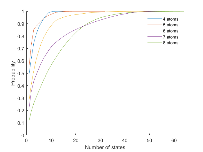
(a)

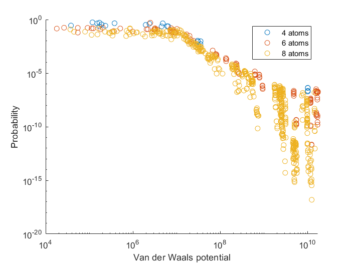
(b)

Figure 6: Figure (a) shows the cumulative probability of states in the solution of the Schrödinger equation in the jamming limit without using state truncation for $\Omega=$5.8\text{\,}\mathrm{MHz}$$, $C_{6}=$50\text{\,}\mathrm{G}\mathrm{Hz}\mathrm{\SIUnitSymbolMicro}\mathrm{m}^{6}$$, and $\rho=$0.031\text{\,}\mathrm{\SIUnitSymbolMicro}\mathrm{m}^{-2}$$. The states are in order of decreasing probability. Figure (b) shows the probability of a state in the solution of the Schrödinger equation in the jamming limit without using state truncation over its Van der Waals potential.

We also observe that the probability a state occurs is negatively correlated with its contribution to the Hamiltonian due to the Van der Waals interaction. Figure 6(b) shows the probability a state occurs as a function of its Van der Waals potential. Clearly the probability diminishes for larger values of the Van der Waals potential. For our simulation we have truncated all states with a Van der Waals potential higher than $10^{8}$ resulting in a truncation of states with a probability of less than $10^{-4}$ of occurring. To verify we computed the maximum absolute difference between the mean number of excitations over time for a small truncated system and the statistics obtained without truncation and observed only fractional differences in all cases, confirming that the truncation does not influence our observations in any significant way.

After truncating the state space, each state is ordered lexicographically in the truncated state space such that it can equivalently be represented by an index $\pi(s)\in\mathbbm{N}$. We then compute the Hamiltonian matrix $H$. An element in the matrix $H_{i,j}$ is computed by determining the interaction energy of the states $s,s^{\prime}\in S$ corresponding to the indices $i,j$. To compute the interaction energy the input parameters and the position matrix $r$ are used as stated in the main text. The Hamiltonian matrix results in the Schrödinger equation which we solve numerically as an ordinary system of differential equations.

References

• [1] M. D. Lukin, M. Fleischhauer, R. Cote, L. M. Duan, D. Jaksch, J. I. Cirac, and P. Zoller, “Dipole blockade and quantum information processing in mesoscopic atomic ensembles,” Phys. Rev. Lett., vol. 87, p. 037901, 6 2001.
• [2] D. Jaksch, J. I. Cirac, P. Zoller, S. L. Rolston, R. Côté, and M. D. Lukin, “Fast quantum gates for neutral atoms,” Phys. Rev. Lett., vol. 85, pp. 2208–2211, 9 2000.
• [3] H. Weimer, R. Löw, T. Pfau, and H. P. Büchler, “Quantum critical behavior in strongly interacting Rydberg gases,” Phys. Rev. Lett., vol. 101, p. 250601, 12 2008.
• [4] D. Comparat and P. Pillet, “Dipole blockade in a cold Rydberg atomic sample,” J. Opt. Soc. Am. B, vol. 27, no. 6, pp. A208–A232, 2010.
• [5] M. Saffman, T. G. Walker, and K. Mølmer, “Quantum information with Rydberg atoms,” Rev. Mod. Phys., vol. 82, pp. 2313–2363, 8 2010.
• [6] T. Cubel Liebisch, A. Reinhard, P. R. Berman, and G. Raithel, “Atom counting statistics in ensembles of interacting Rydberg atoms,” Phys. Rev. Lett., vol. 95, p. 253002, 12 2005.
• [7] M. Viteau, P. Huillery, M. G. Bason, N. Malossi, D. Ciampini, O. Morsch, E. Arimondo, D. Comparat, and P. Pillet, “Cooperative excitation and many-body interactions in a cold Rydberg gas,” Phys. Rev. Lett., vol. 109, p. 053002, 7 2012.
• [8] C. S. Hofmann, G. Günter, H. Schempp, M. Robert-de-Saint-Vincent, M. Gärttner, J. Evers, S. Whitlock, and M. Weidemüller, “Sub-poissonian statistics of Rydberg-interacting dark-state polaritons,” Phys. Rev. Lett., vol. 110, p. 203601, 5 2013.
• [9] N. Malossi, M. M. Valado, S. Scotto, P. Huillery, P. Pillet, D. Ciampini, E. Arimondo, and O. Morsch, “Full counting statistics and phase diagram of a dissipative Rydberg gas,” Phys. Rev. Lett., vol. 113, p. 023006, 7 2014.
• [10] P. Schauß, J. Zeiher, T. Fukuhara, S. Hild, M. Cheneau, T. Macrì, T. Pohl, I. Bloch, and C. Gross, “Crystallization in ising quantum magnets,” Science, vol. 347, no. 6229, pp. 1455–1458, 2015.
• [11] F. Letscher, O. Thomas, T. Niederprüm, M. Fleischhauer, and H. Ott, “Bistability vs. metastability in driven dissipative rydberg gases,” arXiv preprint arXiv:1611.00627, 2016.
• [12] IOPScience, “Special issue on Rydberg atomic physics,” Journal of Physics B, 2016.
• [13] F. Robicheaux and J. V. Hernández, “Many-body wave function in a dipole blockade configuration,” Phys. Rev. A, vol. 72, p. 063403, 12 2005.
• [14] M. Höning, D. Muth, D. Petrosyan, and M. Fleischhauer, “Steady-state crystallization of Rydberg excitations in an optically driven lattice gas,” Phys. Rev. A, vol. 87, p. 023401, Feb. 2013.
• [15] D. Petrosyan, “Dynamics and equilibration of Rydberg excitations in dissipative atomic ensembles,” arXiv e-print 1305.2341, 2013.
• [16] C. Ates, T. Pohl, T. Pattard, and J. M. Rost, “Many-body theory of excitation dynamics in an ultracold Rydberg gas,” Phys. Rev. A, vol. 76, p. 013413, 7 2007.
• [17] C. Ates, S. Sevinçli, and T. Pohl, “Electromagnetically induced transparency in strongly interacting Rydberg gases,” Phys. Rev. A, vol. 83, p. 041802, Apr. 2011.
• [18] D. Petrosyan, M. Höning, and M. Fleischhauer, “Spatial correlations of Rydberg excitations in optically driven atomic ensembles,” Physical Review A, vol. 87, no. 5, p. 053414, 2013.
• [19] C. Ates and I. Lesanovsky, “Entropic enhancement of spatial correlations in a laser-driven Rydberg gas,” Phys. Rev. A, vol. 86, p. 013408, 7 2012.
• [20] J. Sanders, M. Jonckheere, and S. Kokkelmans, “Sub-Poissonian statistics of jamming limits in ultracold rydberg gases,” Physical Review Letters, vol. 115, no. 4, p. 043002, 2015.
• [21] H. Wu, Y. Li, Z.-B. Yang, and S.-B. Zheng, “Quantum signature for laser-driven correlated excitation of Rydberg atoms,” Physical Review A, vol. 95, no. 1, p. 013842, 2017.
• [22] C. Pérez-Espigares, I. Lesanovsky, J. P. Garrahan, and R. Gutiérrez, “Glassy dynamics due to a trajectory phase transition in dissipative rydberg gases,” Physical Review A, vol. 98, no. 2, p. 021804, 2018.
• [23] R. Gutiérrez, J. P. Garrahan, and I. Lesanovsky, “Physical swap dynamics, shortcuts to relaxation, and entropy production in dissipative rydberg gases,” Physical Review E, vol. 100, no. 1, p. 012110, 2019.
• [24] V. R. Overbeck, M. F. Maghrebi, A. V. Gorshkov, and H. Weimer, “Multicritical behavior in dissipative ising models,” Physical Review A, vol. 95, no. 4, p. 042133, 2017.
• [25] M. Foss-Feig, J. T. Young, V. V. Albert, A. V. Gorshkov, and M. F. Maghrebi, “Solvable family of driven-dissipative many-body systems,” Physical review letters, vol. 119, no. 19, p. 190402, 2017.
• [26] K. Macieszczak, D. C. Rose, I. Lesanovsky, and J. P. Garrahan, “Theory of classical metastability in open quantum systems,” arXiv preprint arXiv:2006.01227, 2020.
• [27] T. Pistorius, J. Kazemi, and H. Weimer, “Quantum many-body dynamics of driven-dissipative rydberg polaritons,” arXiv preprint arXiv:2003.10463, 2020.
• [28] J. W. Evans, “Random and cooperative sequential adsorption,” Rev. Mod. Phys., vol. 65, pp. 1281–1329, 10 1993.
• [29] B. Senger, J.-C. Voegel, and P. Schaaf, “Irreversible adsorption of colloidal particles on solid substrates,” Colloids and Surfaces A: Physicochemical and Engineering Aspects, vol. 165, no. 1-3, pp. 255–285, 2000.
• [30] A. Rényi, “On a one-dimensional random space-filling problem,” MTA Mat Kut. Int. Kzl, vol. 3, pp. 109–127, 1958.
• [31] P. Erdös and A. Rényi, “On random graphs, I,” Publicationes Mathematicae (Debrecen), vol. 6, pp. 290–297, 1959.
• [32] S. Dhara, J. S. van Leeuwaarden, and D. Mukherjee, “Generalized random sequential adsorption on erdős–rényi random graphs,” Journal of Statistical Physics, vol. 164, no. 5, pp. 1217–1232, 2016.
• [33] P. Bermolen, M. Jonckheere, and P. Moyal, “The jamming constant of uniform random graphs,” Stochastic Processes and their Applications, vol. 127, no. 7, pp. 2138–2178, 2017.
• [34] P. Bermolen, M. Jonckheere, and J. Sanders, “Scaling limits and generic bounds for exploration processes,” Journal of Statistical Physics, vol. 169, no. 5, pp. 989–1018, 2017.
• [35] S. Dhara, J. S. van Leeuwaarden, and D. Mukherjee, “Corrected mean-field model for random sequential adsorption on random geometric graphs,” Journal of Statistical Physics, vol. 173, no. 3-4, pp. 872–894, 2018.
• [36] M. Jonckheere and M. Sáenz, “Asymptotic optimality of degree-greedy discovering of independent sets in configuration model graphs,” arXiv preprint arXiv:1808.10358, 2018.
• [37] T. M. Meyfroyt, “Degree-dependent threshold-based random sequential adsorption on random trees,” Advances in Applied Probability, vol. 50, no. 1, p. 302, 2018.
• [38] P. Bermolen, M. Jonckheere, F. Larroca, and M. Saenz, “Sequential algorithms and independent sets discovering on large sparse random graphs,” arXiv preprint arXiv:2009.14574, 2020.
• [39] F. Robicheaux and J. Hernández, “Many-body wave function in a dipole blockade configuration,” Physical Review A, vol. 72, no. 6, p. 063403, 2005.
• [40] M. P. Fewell, “Area of common overlap of three circles,” tech. rep., Maritime Operations Division, Defence Science and Technology Organisation, Edinburgh (Australia), 2006.
• [41] P. Schauß, M. Cheneau, M. Endres, T. Fukuhara, S. Hild, A. Omran, T. Pohl, C. Gross, S. Kuhr, and I. Bloch, “Observation of spatially ordered structures in a two-dimensional Rydberg gas,” Nature, vol. 491, no. 7422, p. 87, 2012.
• [42] I. Lesanovsky and J. P. Garrahan, “Out-of-equilibrium structures in strongly interacting Rydberg gases with dissipation,” Phys. Rev. A, vol. 90, p. 011603, 7 2014.
• [43] I. Karatzas and S. Shreve, Brownian motion and stochastic calculus, vol. 113. Springer Science & Business Media, 2012.
• [44] R. Liptser and A. N. Shiryayev, Theory of martingales, vol. 49. Springer Science & Business Media, 2012.