TUM-HEP-1291/20

Anomalous Dimensions of Effective Theories
from Partial Waves

Pietro Baratella^a, Clara Fernandez^b, Benedict von Harling^b and Alex Pomarol^b,c

^aTechnische Universität München, Physik-Department, 85748 Garching
^bIFAE and BIST, Universitat Autònoma de Barcelona, 08193 Bellaterra, Barcelona
^cDepartament de Física, Universitat Autònoma de Barcelona, 08193 Bellaterra, Barcelona

1 Introduction

Approaching physical systems by using effective field theories has proven to be quite successful in order to describe their low-energy physical properties. The anomalous dimensions $\gamma_{i}$ play an important role in this approach, since they determine how the parameters of the theory (the Wilson coefficients) vary with the energy scale at which the experiments are carried out. Their calculation is therefore important to extract the relevant properties of the systems, as shown in many examples in hadron physics, the SM or gravity.

Recently, there has been certain activity to show how to calculate anomalous dimensions from on-shell methods [1, 2, 3, 4, 5], following the earlier work of [6, 7, 8]. These methods are equivalent to the ordinary operator approach of effective field theories, since amplitudes can be related one-to-one to higher-dimensional operators. Nevertheless, on-shell methods have been shown to be simpler and more efficient, and also more manageable when going beyond the one-loop order (see for example [2, 9, 4]).

In particular, in Ref. [3] a simple formula was presented for computing anomalous dimensions from a product of tree-level amplitudes, integrated over some phase space. In this paper, we will gain a deeper understanding of the properties of this formula by performing a partial-wave decomposition of the amplitudes. This will allow us to effectively capture the information contained in the conservation of angular momentum (see also [10] for related work). As we will see in detail, angular-momentum analysis allows us to reduce the phase-space integrals in [3] to a product of two partial-wave coefficients, $a^{J}_{L}a^{J}_{R}$, summed over the angular momenta $J$. The key observation is that, for contact interactions (in particular, those related to higher-dimensional operators), only one or a few $J$s contribute to the decomposition, so that the sum over $J$ has a reduced number of terms. In other words, the non-trivial information necessary to obtain the anomalous dimension is contained in a few partial-wave coefficients.

The traditional arena for using partial-wave analysis is two-to-two scatterings or, equivalently, 4-point amplitudes, where the method is already quite developed [11]. In this article, we will restrict ourselves to these amplitudes, as they are also the important ones in many theories of interest. The generalization to higher-point amplitudes can however be easily obtained by following the lines of [10]. The presence of IR divergencies in the renormalization of amplitudes will also be considered, and we will see that this requires a regularization of the partial-wave coefficients.

We will present various applications of our results. First, we will consider the SM EFT and calculate several anomalous dimensions. We will see that, in a class of 4-point amplitudes with equal total helicity, the partial-wave coefficient which is needed to calculate the one-loop mixings is essentially the same. After that, we will see that our approach also allows us to obtain a generic formula for the anomalous dimensions of nonlinear sigma models at any order in the energy expansion. Finally, we will show how the calculations in gravity are even simpler than in the previous examples, and definitely much simpler than in the ordinary Feynman approach.

2 Anomalous dimensions from partial-wave amplitudes

In this work, we follow the on-shell amplitude approach, and define a theory by its particle content and scattering amplitudes. Higher-point amplitudes are constructed from lower-point ones, with the ones with the least points playing the role of building-blocks of the theory. In low-energy EFfective Theories (EFTs), the set of “building-block” amplitudes ${\cal A}_{i}$ is constructed according to an expansion in $E/\Lambda$, where $\Lambda$ is some UV cut-off of the EFT. Here, we will be considering EFTs with only massless states, and follow the spinor-helicity notation [12]. For scalars, fermions, gauge bosons and gravitons, the leading term in the $E/\Lambda$ expansion is given by 3-point amplitudes (which can in general be non-local) defined at complex momenta. From these, one can build for example all amplitudes of gauge theories. At higher order in $E/\Lambda$, the amplitudes ${\cal A}_{i}$ correspond to contact interactions, which will be the subject of our interest. Among them, we will focus on 3-point and 4-point amplitudes.

The independent coefficients of the building-block amplitudes ${\cal A}_{i}$, which we denote as $C_{i}$, are the “couplings” of the EFT, which must of course be determined experimentally. They are renormalized at the loop level, receiving anomalous dimensions $\gamma_{i}$. We want to show that these anomalous dimensions at the one-loop level can easily be determined from products of partial-wave amplitudes.

2.1 One-loop anomalous dimensions via on-shell amplitudes

Let us start by considering the case in which there are no IR divergencies. It was shown in [3] that, in this situation, the one-loop anomalous dimension of an amplitude $\gamma_{i}$ can be written as a product of tree-level amplitudes under a phase-space integration. Defining $\gamma_{i}=dC_{i}/d\ln\mu$, we find for the particular case of 4-point amplitudes that [3]

$$\gamma_{i}\frac{{\cal A}_{i}(1,2,3,4)}{C_{i}}=-\frac{1}{4\pi^{3}}\int d{\rm LIPS}\sum_{1^{\prime},2^{\prime}}\sigma_{1^{\prime}2^{\prime}}\Big{[}{\cal A}_{L}(1,2,{\bar{2}^{\prime}},{\bar{1}^{\prime}}){\cal A}_{R}(1^{\prime},2^{\prime},3,4)\Big{]}+(2\leftrightarrow 3)+(2\leftrightarrow 4)\,.$$ (1)

Here ${\cal A}_{L,R}$ are 4-point tree-level amplitudes (with all states incoming), which are constructed using the building-block amplitudes ${\cal A}_{j}$. Their exponent in $1/\Lambda$, which we denote as $w$, i.e. ${\cal A}\propto 1/\Lambda^{w}$, must satisfy

$$w_{i}=w_{L}+w_{R}\,.$$ (2)

The three terms in Eq. (1) arise from 2-cuts of the one-loop amplitude in respectively the $s$-, $t$- and $u$-channel. The sum $\sum_{1^{\prime},2^{\prime}}$ in Eq. (1) is taken over amplitudes ${\cal A}_{L,R}$ with all possible internal states $1^{\prime},2^{\prime}$ (and over quantum numbers such as color or flavor). The bar over a state (e.g. $\bar{1}$) indicates that it carries opposite-sign momentum, helicity and all other quantum numbers with respect to the state without a bar (e.g. $1$). When writing down amplitudes in the spinor-helicity formalism (as we do here), one needs a prescription for $\left|-p\right\rangle$ and $\left|-p\right]$. Here we take $\left|-p\right\rangle=i|p\rangle$ and $\left|-p\right]=i|p]$ [3]. In this convention, the factor $\sigma_{1^{\prime}2^{\prime}}$ is defined by $\sigma_{i_{1}i_{2}}\equiv(-i)^{F_{i_{1}i_{2}}}$, where $F_{i_{1}i_{2}}$ counts the number of fermions in the list $\{i_{1}i_{2}\}$. A factor 1/2 must also be included in Eq. (1) when the internal particles are indistinguishable.

Before proceeding, let us point out simple generalizations of Eq. (1) which we will use in the examples of Sec. 3. Firstly, it is quite common to have more than one independent amplitude ${\cal A}_{i}$ with the same 4 external states. In this case, we have a sum over the corresponding indices $i$ on the LHS of Eq. (1). Secondly, the ${\cal A}_{i}$ in Eq. (1) does not necessarily have to be a building-block amplitude. Instead, it can be a 4-point amplitude made from 3-point building-blocks. In this case, we will denote it as $\widehat{\cal A}_{i}$. We will see an example of this in the context of gravity, where we will study the renormalization of the 3-point amplitude made of equal-helicity gravitons, ${\cal A}_{R^{3}}$, from the renormalization of a 4-point amplitude containing it, which we call $\widehat{\cal A}_{R^{3}}$.

As a next step, we will perform a decomposition into the angular momenta $J$ of the internal state, the particle pair $1^{\prime},2^{\prime}$ (and, similarly, decompose it according to its other quantum numbers such as isospin). For a given $J$ of the $1^{\prime},2^{\prime}$-system, angular momentum conservation implies that also the external states of ${\cal A}_{L,R}$ must be in the same $J$, and the same for ${\cal A}_{i}$.

The interesting point is that, for contact interactions like ${\cal A}_{i}$ with $w_{i}>0$, only a few $J$-channels contribute, as we will show with some examples. This means that the anomalous dimension in Eq. (1) is determined by only a few $J$-channels, simplifying then its computation. The purpose of the following analysis is to make these statements quantitative, finding out explicitly what angular momenta $J$ mediate the anomalous dimensions.

2.2 Partial-wave decomposition

In order to perform the angular-momentum decomposition of an amplitude ${\cal A}(1_{h_{1}},2_{h_{2}},3_{h_{3}},4_{h_{4}})$, with $h_{i}$ denoting the helicity of particle $i$, it is convenient to specify the pair of incoming and outgoing states. Let us for concreteness consider the $s$-channel, i.e. $1_{h_{1}},2_{h_{2}}\to 3_{-h_{3}},4_{-h_{4}}$. We define

$${\cal A}(1_{h_{1}},2_{h_{2}}\to 3_{-h_{3}},4_{-h_{4}})\equiv\sigma_{34}\,{\cal A}(1_{h_{1}},2_{h_{2}},-4_{h_{4}},-3_{h_{3}})\,,$$ (3)

where the factor $\sigma_{34}$ when crossing fermions arises in our convention where $\left|-p\right\rangle=i|p\rangle$ and $\left|-p\right]=i|p]$. Notice that, in terms of the ‘bar’ notation previously introduced, one has for example $\overline{(1_{h_{1}})}=-1_{-h_{1}}$. By going to the center-of-momentum frame and aligning the $z$-axis with the direction of particles 1 and 2 (with $\vec{p}_{1}$ pointing downwards), we can parametrize the direction of the outgoing particle $4$ by the polar coordinates $(\theta,\phi)$. The amplitude can then be written as a function of the two polar angles and the Mandelstam variable $s$:

$${\cal A}(1_{h_{1}},2_{h_{2}}\to 3_{-h_{3}},4_{-h_{4}})={\cal A}(s,\theta,\phi)\,.$$ (4)

When the amplitude is given in spinor-helicity notation, this frame corresponds to taking (notice that here $p_{1}+p_{2}=p_{3}+p_{4}$)

$$\begin{array}[]{l}|3\rangle=c_{\theta/2}|1\rangle-s_{\theta/2}e^{-i\phi}|2\rangle\\ |4\rangle=s_{\theta/2}e^{i\phi}|1\rangle+c_{\theta/2}|2\rangle\end{array},\quad\ \ \begin{array}[]{l}|3]=c_{\theta/2}|1]-s_{\theta/2}e^{i\phi}|2]\\ |4]=s_{\theta/2}e^{-i\phi}|1]+c_{\theta/2}|2]\end{array},$$ (5)

where $s_{\theta/2}\equiv\sin\theta/2$ and $c_{\theta/2}\equiv\cos\theta/2$. Furthermore, we have $\langle 12\rangle=[21]=\sqrt{s}$, while the Mandelstam variables $t=-\langle 13\rangle[31]$ and $u=-\langle 14\rangle[41]$ become

$$t=-s\,\frac{1-c_{\theta}}{2}\ ,\quad\quad u=-s\,\frac{1+c_{\theta}}{2}\,.$$ (6)

To exploit the information contained in the conservation of angular momentum, we can now perform a partial-wave decomposition of the initial and final states of ${\cal A}$ in Eq. (4) (on a basis having definite angular momentum, quantized along the $z$-axis). This gives [11] (see details in Appendix B)

$${\cal A}(s,\theta,\phi)=e^{i\phi(h_{12}-h_{43})}\left(\frac{\sqrt{s}}{\Lambda}\right)^{w}\sum_{J}n_{J}\,d_{h_{12}h_{43}}^{J}(\theta)\,a^{J},$$ (7)

where $n_{J}=2J+1$, $h_{12}=h_{1}-h_{2}$ (and similarly for $h_{43}$), and where $d_{hh^{\prime}}^{J}(\theta)$ are the Wigner $d$-functions. Notice that we have factored out the dependence of the amplitude on $\sqrt{s}/\Lambda$. The partial-wave expansion, Eq. (7), can be inverted to give the coefficients $a^{J}$ for the amplitude:

$$a^{J}=\frac{1}{2}\left(\frac{\sqrt{s}}{\Lambda}\right)^{-w}\int_{0}^{\pi}d\theta\,s_{\theta}\,d_{h_{12}h_{43}}^{J}(\theta)\,{\cal A}(s,\theta,\phi=0)\,,$$ (8)

where we have used the orthogonality of the Wigner $d$-functions (see Eq. (74) in Appendix B). The above derivation implicitly assumes the existence of well-defined coefficients $a^{J}$, which is not always guaranteed, as we will see in Sec. 2.3.

In the same way as for the $s$-channel, we can perform a partial-wave decomposition for the $t$-channel $1,3\to{2,4}$ and the $u$-channel $1,4\to{3,2}$. This leads to the same expression as Eq. (7), with the replacements $(2\leftrightarrow 3)$ and $(2\leftrightarrow 4)$ respectively. In this case, the polar angles give the direction of the outgoing pairs $2,4$ and $3,2$ respectively. The coefficients $a^{J}$, either derived in the $s$-, $t$- or $u$-channel, completely characterize the amplitude ${\cal A}(1,2,3,4)$. Depending on the problem under consideration, we can use one or another. We can also write Eq. (7) in a manifestly Lorentz-invariant form by inverting Eq. (6), which leads to $c_{\theta}=(t-u)/s$, while in the $t$- and $u$-channel we have $c_{\theta}=(s-u)/t$ and $c_{\theta}=(t-s)/u$, respectively.

Let us now consider the phase-space integrations in Eq. (1), and apply a partial-wave decomposition to ${\cal A}_{L}$ and ${\cal A}_{R}$ with respect to the $J$ of the two external states. This corresponds to decomposing ${\cal A}_{L,R}$ in the first term of Eq. (1) in the $s$-channel, specifically $1,2\to 1^{\prime},2^{\prime}$ and $1^{\prime},2^{\prime}\to\bar{4},\bar{3}$. Let us show in detail how this proceeds. We denote the polar angles which give the $1^{\prime},2^{\prime}$-direction as $(\theta^{\prime},\phi^{\prime})$, and those for the $\bar{4},\bar{3}$-direction as $(\theta,\phi)$. The phase-space integral for $1^{\prime},2^{\prime}$ in Eq. (1) then reduces to an angular integration over the primed polar coordinates, that is $\int d{\rm LIPS}=\int d\theta^{\prime}s_{\theta^{\prime}}d\phi^{\prime}/8$. Using Eq. (71) of Appendix B, we find

$$\int d{\rm LIPS}~{}\sigma_{1^{\prime}2^{\prime}}{\cal A}_{L}(1,2,\bar{2}^{\prime},\bar{1}^{\prime}){\cal A}_{R}(1^{\prime},2^{\prime},3,4)=\int d{\rm LIPS}~{}{\cal A}_{L}(1,2\to 1^{\prime},2^{\prime})\,\sigma_{34}^{-1}{\cal A}_{R}(1^{\prime},2^{\prime}\to\bar{4},\bar{3})$$

$$=\frac{1}{8}\,\sigma_{34}^{-1}\left(\frac{\sqrt{s}}{\Lambda}\right)^{w_{L}+w_{R}}\int_{0}^{\pi}d\theta^{\prime}s_{\theta^{\prime}}\int_{0}^{2\pi}d\phi^{\prime}\,\sum_{J^{\prime}}n_{J^{\prime}}\,e^{i\phi^{\prime}(h_{12}-h^{\prime}_{12})}d_{h_{12}h^{\prime}_{12}}^{J^{\prime}}(\theta^{\prime})\,a_{L}^{J^{\prime}}$$

$$\hskip 96.73918pt\times\sum_{JM}n_{J}\,e^{i\phi(M-h_{34})}d_{Mh_{34}}^{J}(\theta)e^{-i\phi^{\prime}(M-h^{\prime}_{12})}d_{Mh^{\prime}_{12}}^{J}(\theta^{\prime})\,a_{R}^{J}$$

$$=\frac{\pi}{2}\,\sigma_{34}^{-1}\,e^{i\phi(h_{12}-h_{34})}\left(\frac{\sqrt{s}}{\Lambda}\right)^{w_{L}+w_{R}}\sum_{J}n_{J}\,d^{J}_{h_{12}h_{34}}(\theta)\,a_{L}^{J}a_{R}^{J}\,,$$ (9)

where in the last step we have performed a trivial $d\phi^{\prime}$ integration and used the orthogonality condition of the Wigner $d$-functions (Eq. (74) of Appendix B). Similarly, we can proceed as above for the second and third term of Eq. (1), which in this case must be decomposed in the $t$- and $u$-channel respectively. Inserting the result in Eq. (1), we obtain

$$\gamma_{i}\frac{{\cal A}_{i}}{C_{i}}=-\frac{1}{8\pi^{2}}\,\sigma_{34}^{-1}\,e^{i\phi(h_{12}-h_{34})}\,\left(\frac{\sqrt{s}}{\Lambda}\right)^{w_{L}+w_{R}}\sum_{J}n_{J}\,d^{J}_{h_{12}h_{34}}(\theta)\sum_{1^{\prime}2^{\prime}}a_{L}^{J}a_{R}^{J}+t\text{-channel}+u\text{-channel}\,.$$ (10)

The sum over $J$ can in principle be infinite. Nevertheless, 4-point amplitudes ${\cal A}_{i}$ with $w>0$ (which are contact interactions) have a finite number of partial waves (the incoming states can only be in a few $J$s), implying that also the RHS of Eq. (10) consists of a finite number of nonzero terms. In most of the cases this is true because only a few coefficients $a^{J}_{L}$ or $a^{J}_{R}$ are nonzero, which makes Eq. (10) a very simple formula to calculate anomalous dimensions. But this is not always the case. Indeed, it is still possible that an infinite series in $J$ appears on the RHS of Eq. (10). When this happens, a non-trivial cancellation between the 3 different channels takes place, such that only a finite number of $J$ contributions remain on the RHS as expected. This occurs however only in a few circumstances, as we will discuss at the end of Sec. 3.1.

Eq. (10) simplifies enormously in certain cases. For example, if there are only contributions from one channel, say the $s$-channel, we can expand the amplitude ${\cal A}_{i}$ on the LHS of Eq. (10) into partial waves in the same channel. From this we get

$$\gamma_{i}\frac{a_{i}^{J}}{C_{i}}=-\frac{1}{8\pi^{2}}\sum_{1^{\prime}2^{\prime}}\,a_{L}^{J}a_{R}^{J}\,.$$ (11)

When several ${\cal A}_{i}$ contribute on the LHS of Eq. (10), we instead have a sum over the corresponding indices $i$ on the LHS of Eq. (11), leading to a system of equations (obtained by projecting on the corresponding quantum numbers of the ${\cal A}_{i}$) that must be solved to obtain the individual $\gamma_{i}$. We will see an example in Sec. 3.2. We further note that $\sigma_{34}^{-1}$ drops out in Eq. (11).

A similar simplification arises when the contribution from each channel is independently proportional to a single ${\cal A}_{i}$. This occurs, for example, when each channel gives a contribution that is parametrically independent from the others (because each depends on different couplings). In this case, we can write

$$\gamma_{i}=\gamma^{s}_{i}+\gamma^{t}_{i}+\gamma^{u}_{i}\,,$$ (12)

where $\gamma_{i}^{s,t,u}$ is the contribution from the $s$-,$t$-,$u$-channel respectively. For the $s$-channel, this contribution is given by

$$\gamma^{s}_{i}\frac{{\cal A}_{i}}{C_{i}}=-\frac{1}{8\pi^{2}}\,\sigma_{34}^{-1}\,e^{i\phi(h_{12}-h_{34})}\left(\frac{\sqrt{s}}{\Lambda}\right)^{w_{L}+w_{R}}\sum_{J}n_{J}\,d^{J}_{h_{12}h_{34}}(\theta)\sum_{1^{\prime}2^{\prime}}\,a_{L}^{J}a_{R}^{J}\,.$$ (13)

After expanding ${\cal A}_{i}$ into partial waves in the $s$-channel, Eq. (13) leads to

$$\gamma^{s}_{i}=-\frac{C_{i}}{8\pi^{2}}\sum_{1^{\prime}2^{\prime}}\frac{a_{L}^{J}a_{R}^{J}}{a_{i}^{J}}\,.$$ (14)

In a similar way, we can proceed for the contributions from the other channels.

Although these particular cases could look very special, they are actually quite common. For example, in the SM EFT most of the renormalizations of 4-point amplitudes at $O(E^{2}/\Lambda^{2})$ can only proceed through one partial wave in one channel, as we will see in the examples of Sec. 3.1. On the other hand, for EFTs of Goldstone bosons or gravitons, we will have to add the three channels together as in Eq. (10). Nevertheless, we will only need to calculate the $s$-channel contribution, since the other channels are determined by crossing symmetry.

2.3 IR divergencies

There are certain cases in which the $d$LIPS integral in Eq. (1) is divergent and must be regulated. This is due to the singular behavior of either $\mathcal{A}_{L}$ or $\mathcal{A}_{R}$ in the limit $\theta\to 0$ or $\theta\to\pi$ (or both), with the amplitude going respectively like $\mathcal{A}\sim s_{\theta/2}^{-2}~{}{\rm or~{}}c_{\theta/2}^{-2}~{}{\rm(or~{}}s_{\theta}^{-2})$. We will focus for the moment on the first case, and later on will comment on the last case. The second case, with singularities only for $\theta\to\pi$, can always be excluded by a reordering of legs.

These singularities are intimately related to soft IR divergencies of the loop integral, as explained in Appendix A. There, we show that in the presence of $\theta\to 0$ soft IR divergencies, Eq. (1) must be corrected by adding the following expression:

$$\Delta\gamma_{i}\,\frac{{\cal A}_{i}(1^{a},2^{b},3^{c},4^{d})}{C_{i}}\,=\,-\frac{1}{4\pi^{3}}\left[({\bm{T}}_{\rm soft}^{12})_{\hat{a}\,\hat{b}}^{a\,b}\,{\cal A}_{R}(1^{\hat{a}},2^{\hat{b}},3^{c},4^{d})\,\int d{\rm LIPS}_{12}\,\frac{1}{s_{\theta^{\prime}\!/2}^{2}}\right.\\ \left.+\,({\bm{T}}_{\rm soft}^{34})_{\hat{c}\,\hat{d}}^{c\,d}\,{\cal A}_{L}(1^{{a}},2^{{b}},3^{\hat{c}},4^{\hat{d}})\,\int d{\rm LIPS}_{34}\,\frac{1}{s_{\theta^{\prime}\!/2}^{2}}\right]+(2\leftrightarrow 3)+(2\leftrightarrow 4)\,,$$ (15)

where the $d$LIPS_ij integrals are over the $i^{\prime}j^{\prime}$-state phase space. Eq. (15) acts as a regulator for the small-angle divergencies contained in Eq. (1). The soft operator ${\bm{T}}_{\rm soft}^{ij}$ can in general act on color/flavor indices $a,b,c,d$ and contains couplings and powers of $s_{ij}=(p_{i}+p_{j})^{2}$. In the simplest cases, like QED or gravity, it is diagonal in color/flavor, i.e. ${\bm{T}}_{\rm soft}\propto\delta_{a\hat{a}}\,\delta_{b\hat{b}}$ (see Appendix A for explicit expressions and the example at the end of Sec. 3.1).

When an amplitude features small-angle singularities, its coefficients $a^{J}$ are logarithmically divergent. Nevertheless, there is a natural generalization of Eq. (8) which consists in defining “regularized” partial-wave coefficients as

$$a^{J}|_{\rm reg}=\frac{1}{2}\left(\frac{\sqrt{s}}{\Lambda}\right)^{-w}\int^{\pi}_{0}d\theta\,s_{\theta}\left(d^{J}_{h_{12}h_{43}}(\theta){\cal A}(1_{h_{1}}^{a},2_{h_{2}}^{b}\to{3}_{-h_{3}}^{c},{4}_{-h_{4}}^{d})|_{\theta,\phi=0}+\frac{\left({\bm{T}}_{\rm soft}\right)^{a\,b}_{c\,d}}{s^{2}_{\theta/2}}\right)\,.$$ (16)

In terms of these coefficients, the anomalous dimensions can still be written as in Eq. (10). Eq. (16) can be inferred in the following way. Let us assume that one of the amplitudes, either $\mathcal{A}_{L}$ or $\mathcal{A}_{R}$, has divergent coefficients $a^{J}$, while for the other one all partial-wave coefficients are finite. Notice that the latter assumption is always fulfilled for contact interactions like the EFT amplitudes ${\cal A}_{i}$ described above. For concreteness, we take $\mathcal{A}_{R}$ to have all coefficients finite. In this case, the $d$LIPS integrals of Eq. (1), together with those of Eq. (15), can be written as

$$\int d{\rm LIPS}\left(\sigma_{1^{\prime}2^{\prime}}\,{\cal A}_{L}(1,2,\bar{2}^{\prime},\bar{1}^{\prime}){\cal A}_{R}(1^{\prime},2^{\prime},3,4)+\frac{{\bm{T}}_{\rm soft}}{s^{2}_{\theta^{\prime}\!/2}}{\cal A}_{R}(1,2,3,4)\right)$$

$$\ \ =\frac{\pi}{2}\,\sigma_{34}^{-1}\,e^{i\phi(h_{12}-h_{34})}\!\left(\frac{\sqrt{s}}{\Lambda}\right)^{w_{R}}\!\sum_{J}n_{J}\,d_{h_{12}h_{34}}^{J}(\theta)\,a_{R}^{J}~{}\frac{1}{2}\!\int_{0}^{\pi}\!d\theta^{\prime}s_{\theta^{\prime}}\!\left(d^{J}_{h_{12}h^{\prime}_{12}}(\theta^{\prime}){\cal A}_{L}\smash{(s,\theta^{\prime},0)}+\frac{{\bm{T}}_{\rm soft}}{s^{2}_{\theta^{\prime}\!/2}}\right)$$

$$\ \ =\frac{\pi}{2}\,\sigma_{34}^{-1}\,e^{i\phi(h_{12}-h_{34})}\left(\frac{\sqrt{s}}{\Lambda}\right)^{w_{R}+w_{L}}\sum_{J}n_{J}\,d_{h_{12}h_{34}}^{J}(\theta)\,a_{R}^{J}\,a_{L}^{J}|_{\rm reg}\,,$$ (17)

where we have left color/flavor indices implicit. Eq. (17) gives the generalization of Eq. (2.2) when there are soft IR divergencies. In other words, when the coefficients $a^{J}$ of an amplitude are ill-defined, signaling the presence of soft IR divergencies, we can still use Eq. (10), but with the regularized coefficients given in Eq. (16). We will see examples in the next section.

We comment now on the possibility that amplitudes have singularities for both $\theta\to 0$ and $\theta\to\pi$, i.e. ${\cal A}\sim 1/s^{2}_{\theta}$, which happens when the particles $1^{\prime}$ and $2^{\prime}$ are identical. In this case, the divergent integral $\int s^{-2}_{\theta^{\prime}\!/2}$ in Eq. (16) must be replaced by $2\int s^{-2}_{\theta^{\prime}}$ to make the integrand well-behaved (see Appendix A). Moreover, Eq. (16) has to be evaluated only for even $J$, since the coefficients $a^{J}$ for odd $J$ are zero and do not need a subtraction.

When also collinear IR divergencies are present in the one-loop amplitude, one must add the extra contribution (see Appendix A)

$$\Delta\gamma_{i}\,\frac{{\cal A}_{i}(1,2,3,4)}{C_{i}}=\gamma_{\rm coll}\,{\cal A}_{i}(1,2,3,4)\,.$$ (18)

This is always diagonal in amplitude space and depends only on the external legs, so that $\gamma_{\rm coll}=\sum_{n=1}^{4}\gamma_{\rm coll}^{(n)}$, where the $\gamma_{\rm coll}^{(n)}$ are given for example in [2, 5].

3 Applications

3.1 The Standard Model EFT

In Refs. [3, 2, 4, 5], several examples of the calculation of the anomalous dimensions in the SM EFT via on-shell amplitude methods were presented. In particular, in [3] the renormalization of the electron dipole operator was provided, and a similarity was shown in the contributions to the anomalous dimension coming from very different Feynman diagrams. As we will see, the angular-momentum analysis clarifies the origin of this similarity.

As a first example, let us consider the one-loop mixing between 4-point amplitudes of total helicity $h=-2$ at $O(E^{2}/\Lambda^{2})$:

$${\cal A}_{WHle}(1_{e},2_{l_{j}},3_{W^{a}_{-}},4_{H^{\dagger}_{i}}) =\frac{C_{WHle}}{\Lambda^{2}}\langle 31\rangle\langle 32\rangle(T^{a})_{ij}\,,$$ (19)

$${\cal A}_{eluq,0}(1_{e},2_{l_{i}},3_{u},4_{q_{j}}) =\frac{C_{eluq,0}}{\Lambda^{2}}\langle 12\rangle\langle 34\rangle\,\epsilon_{ij}\,,$$

$${\cal A}_{eluq,1}(1_{e},2_{l_{i}},3_{u},4_{q_{j}}) =\frac{C_{eluq,1}}{\Lambda^{2}}\frac{1}{2}\left(\langle 23\rangle\langle 41\rangle+\langle 13\rangle\langle 42\rangle\right)\epsilon_{ij}\,,$$

$${\cal A}_{W^{2}H^{2}}(1_{W_{-}^{a}},2_{H_{j}},3_{W_{-}^{b}},4_{H^{\dagger}_{i}}) =\frac{C_{W^{2}H^{2}}}{\Lambda^{2}}\langle 13\rangle^{2}\delta_{ab}\delta_{ij}\,.$$

Notice that we have chosen ${\cal A}_{eluq,0}$ (${\cal A}_{eluq,1}$) to be antisymmetric (symmetric) with respect to $1\leftrightarrow 2$. As we will see, its only non-vanishing partial-wave component then has $J=0$ ($J=1$). In Eq. (19) there are 3 types of amplitudes which differ by the number of fermions involved, $n_{F}=0,2,4$. We will study the one-loop mixing between these 3 types. Although from the ordinary Feynman approach the anomalous dimensions of Eq. (19) arise from very different diagrams, from on-shell methods we can easily understand that the different mixings are in fact related. Indeed, from Eq. (1) one can realize that the mixings between amplitudes with different $n_{F}$ in Eq. (19) can only proceed through the same type of SM amplitude. This is given by [3]

$${\cal A}_{\rm SM}(1_{\bar{\psi}_{R}},2_{\bar{\psi}_{L_{i}}},3_{W^{a}_{-}},4_{H_{j}})=y_{\psi}\,g_{2}\,(T^{a})_{ij}\frac{\langle 13\rangle\langle 43\rangle}{\langle 14\rangle\langle 12\rangle}\,,$$ (20)

or its complex conjugate, where $\psi_{L}\left(\psi_{R}\right)$ refers to the SM $SU(2)_{L}$-doublet (singlet) lepton, or to the up-type quark upon the replacement $H_{j}\to H^{\dagger}_{j}$ and $(T^{a})_{ij}\to(T^{a})_{ij^{\prime}}\epsilon_{j^{\prime}j}$.

The partial-wave decomposition can tell us even more. First, we notice that the mixing between amplitudes with different $n_{F}$ in Eq. (19) proceeds only through the $s$-channel (no product of amplitudes can be found in the $t$- and $u$-channel which can generate these mixings). The only exception is the renormalization of ${\cal A}_{W^{2}H^{2}}$ by ${\cal A}_{WHle}$, which occurs through both the $s$- and the $t$-channel, but these are trivially related by the crossing of the external $W$ bosons. In the $s$-channel, the partial-wave coefficients of Eq. (20) are given (using Eq. (5)) by

$$a^{J=0}_{\rm SM}=0\,,\ \ \ \ \ a^{J\geq 1}_{\rm SM}={y_{\psi}}g_{2}(T^{a})_{ij}\frac{1}{2}\int_{0}^{\pi}d\theta s_{\theta}\,d_{0,1}^{J}(\theta)\frac{s_{\theta/2}}{c_{\theta/2}}=\frac{{y_{\psi}}g_{2}(T^{a})_{ij}}{\sqrt{J(J+1)}}\,,$$ (21)

while for the amplitudes of Eq. (19) we report them in Table 1. Notice that ${\cal A}_{eluq,0}$, having only a $J=0$ partial-wave component, cannot mix with the rest of the amplitudes which have only $J=1$ components (this angular momentum selection rule was already pointed out in Refs. [10, 3]). The other amplitudes of Eq. (19) can mix among themselves, but always through the $J=1$ partial wave. Therefore all mixings are proportional to $a^{J=1}_{\rm SM}$.

We can explicitly calculate these mixing using Eq. (14). We obtain

$$\begin{pmatrix}\gamma_{WHle}\ C^{-1}_{WHle}a^{1}_{WHle}\\ \gamma_{eluq,1}\ C^{-1}_{eluq,1}a^{1}_{eluq,1}\\ \gamma_{W^{2}H^{2}}\ C^{-1}_{W^{2}H^{2}}a^{1}_{W^{2}H^{2}}\end{pmatrix}=-\frac{\widetilde{a}^{J=1}_{\rm SM}}{8\pi^{2}}\begin{pmatrix}\times&-N_{c}y_{u}&y_{e}\\ -y_{u}&\times&0\\ y_{e}&0&\times\end{pmatrix}\begin{pmatrix}a^{1}_{WHle}\\ a^{1}_{eluq,1}\\ a^{1}_{W^{2}H^{2}}\end{pmatrix}{+\ \text{crossing}}\,,$$ (22)

where we have defined $a^{J}_{\rm SM}=y_{\psi}\widetilde{a}^{J}_{\rm SM}$, and omitted the diagonal entries as they correspond to self-renormalizations which we do not consider here. The crossing accounts for the renormalization of ${\cal A}_{W^{2}H^{2}}$ by ${\cal A}_{WHle}$ in the $t$-channel. This can be easily obtained by just interchanging $W^{a}\leftrightarrow W^{b}$ as the kinematics turns out to be invariant under this crossing. Therefore, in Eq. (22), the matrix in the RHS is trivially determined by color factors, signs due to fermion permutations and different Yukawa couplings. The non-trivial part of the one-loop calculation has gone into the product of the coefficients $a^{1}$ of the amplitudes of Eq. (19) with that of the SM amplitude in Eq. (20). By plugging the values of Table 1 into Eq. (22), we obtain

$$\begin{pmatrix}\gamma_{WHle}\\ \gamma_{eluq,1}\\ \gamma_{W^{2}H^{2}}\end{pmatrix}=\frac{g_{2}}{16\pi^{2}}\begin{pmatrix}\times&N_{c}y_{u}&-2y_{e}\\ \frac{3}{2}y_{u}&\times&0\\ -\frac{1}{2}y_{e}&0&\times\end{pmatrix}\begin{pmatrix}C_{WHle}\\ C_{eluq,1}\\ C_{W^{2}H^{2}}\end{pmatrix}.$$ (23)

This property of all one-loop anomalous dimensions being proportional to the same coefficient $a^{J}_{\rm SM}$ occurs at $O(E^{2}/\Lambda^{2}$) for mixings between 4-point amplitudes with different number of fermions $n_{F}$ and same total helicity $h$. Here, we have shown it for $h=-2$, but the same is true for 4-point amplitudes with $h=0$. In this case, the mixings between amplitudes with different $n_{F}$ are proportional to the $J=1$ partial wave of the SM $\psi\bar{\psi}HH^{\dagger}$ amplitude.

	$J=0$	$J=1$
${\cal A}_{\rm SM}(1_{\bar{\psi}_{R}},2_{\bar{\psi}_{Li}},3_{W^{a}_{-}},4_{H_{j}})$	$0$	$\frac{1}{\sqrt{2}}$	$\times\,y_{\psi}g_{2}\,(T^{a})_{ij}$
${\cal A}^{I=0}_{\rm SM}(1_{H},2_{H^{\dagger}},3_{H^{\dagger}},4_{H})$	$-\frac{3}{8}$	$-\frac{3}{2}$	$\times\,g_{2}^{2}$
${\cal A}_{WHle}(1_{e},2_{l_{j}},3_{W^{a}_{-}},4_{H^{\dagger}_{i}})$	$0$	$\frac{1}{3\sqrt{2}}$	$\times\,C_{WHle}(T^{a})_{ij}$
${\cal A}_{eluq,0}(1_{e},2_{l_{i}},3_{u},4_{q_{j}})$	1	$0$	$\times\,C_{eluq,0}\,\epsilon_{ij}$
${\cal A}_{eluq,1}(1_{e},2_{l_{i}},3_{u},4_{q_{j}})$	$0$	$\frac{1}{6}$	$\times\,C_{eluq,1}\,\epsilon_{ij}$
${\cal A}_{W^{2}H^{2}}(1_{W_{-}^{a}},2_{H_{j}},3_{W_{-}^{b}},4_{H^{\dagger}_{i}})$	$0$	$\frac{1}{3}$	$\times\,C_{W^{2}H^{2}}\delta_{ab}\delta_{ij}$
$\mathcal{A}_{B^{2}H^{2}}(1_{B_{-}},2_{B_{-}},3_{H_{i}},4_{H_{i}^{\dagger}})$	1	0	$\times\,C_{B^{2}H^{2}}$

Table 1: Values of the coefficients $a^{J}$ in the $s$-channel for the different SM amplitudes (up to $J=1$) and SM EFT amplitudes at $O(E^{2}/\Lambda^{2})$ discussed in the text. For ${\cal A}^{I=0}_{\rm SM}$ we give the regularized coefficient $a^{J}|_{\rm reg}$ (see main text).

Let us now consider an example in the SM EFT in which IR divergences are present. In particular, let us calculate the self-renormalization of

$$\mathcal{A}_{B^{2}H^{2}}(1_{B_{-}},2_{B_{-}},3_{H_{i}},4_{H_{i}^{\dagger}})\,=\frac{C_{B^{2}H^{2}}}{\Lambda^{2}}\langle 12\rangle^{2}\,.$$ (24)

We focus on the corrections proportional to $g_{2}$, which arise purely from the $s$-channel. The amplitude Eq. (24) only contributes with $J=0$ and $SU(2)_{L}$ isospin $I=0$ in the $s$-channel. When studying the contributions to the self-renormalization of Eq. (24), we therefore just need to consider the amplitude $\mathcal{A}_{\rm SM}(1_{H},2_{H^{\dagger}},3_{H^{\dagger}},4_{H})$ projected into the zero-isospin channel (due to isospin conservation). This reads

$$\mathcal{A}^{I=0}_{\rm SM}(1_{H},2_{H^{\dagger}},3_{H^{\dagger}},4_{H})=\frac{3}{4}\,g_{2}^{2}\left(\frac{1}{2}+\frac{u}{t}\right).$$ (25)

From Eq. (6), we see that the last term of Eq. (25), which comes from $t$-channel exchanges of $W$s, has a $\theta\to 0$ singularity. Therefore, we have to use the regularized partial-wave coefficients defined in Eq. (16). ${\bm{T}}_{\rm soft}$, once projected into the $I=0$-channel, is given by

$${\bm{T}}^{I=0}_{\rm soft}=-\frac{3}{4}\,g_{2}^{2}\,.$$ (26)

Plugging Eqs. (25) and (26) into Eq. (16), we get $a_{\rm SM}^{J=0}|_{\rm reg}=-3g_{2}^{2}/8$ and $a_{\rm SM}^{J\geq 1}|_{\rm reg}=2H_{J}{\bm{T}}^{I=0}_{\rm soft}$, with $H_{J}$ being the $J$-th harmonic number. Using Eq. (14) together with the collinear contributions in Eq. (18), we obtain

$$\gamma_{B^{2}H^{2}}=-\frac{1}{8\pi^{2}}\,a^{J=0}_{\rm SM}|_{\rm reg}\,C_{B^{2}H^{2}}+\gamma_{\rm coll}C_{B^{2}H^{2}}=-\frac{9}{64\pi^{2}}\,g_{2}^{2}\,C_{B^{2}H^{2}}\,,$$ (27)

where we have also used that $\gamma_{\rm coll}=2\gamma_{\rm coll}^{H}=-3g_{2}^{2}/16\pi^{2}$ [2, 5].

We finish by commenting on certain cases in the SM EFT in which the partial-wave decomposition is not so useful, since the number of terms in the sum in Eq. (10) is infinite. This can occur in the calculation of the renormalization of a 4-point amplitude from a 3-point amplitude. An example can be found in [3]: the renormalization of ${\cal A}_{WHle}$ from ${\cal A}_{W^{3}}(1_{W^{a}_{-}},2_{W^{b}_{-}},3_{W^{c}_{-}})$, given by the amplitudes shown in Fig. 8 of [3]. In this case, both $a^{J}_{L}$ and $a^{J}_{R}$ are nonzero for infinitely many $J$s, a fact which is related to the presence of a logarithm in each channel [3]. When the infinite sums of the different channels are added, only the contribution from a few $J$s remains nonzero, while the rest cancels. This is due to the fact that the logarithms cancel when adding all channels, leaving a constant term proportional to ${\cal A}_{WHle}$. We therefore see that in this particular case, Eq. (10) is not very efficient to calculate the anomalous dimension.

3.2 Nonlinear sigma models

Let us now apply our methods to study the renormalization of nonlinear sigma models. Our analysis will allow us to easily obtain a very general analytic expression for the anomalous-dimension matrix.

From the amplitude perspective, the model is defined as an EFT of real scalars, transforming under some symmetry group, and with amplitudes satisfying Adler’s zero condition [14]: the amplitudes vanish in the limit in which any of the external momenta is taken to zero. For definiteness, we focus on scalars in the fundamental representation of $SO(N)$, and only study 4-point amplitudes in an expansion in $E/\Lambda$. Any 4-point amplitude involving (positive) powers of the external momenta automatically satisfies Adler’s zero condition. Therefore, by starting at $O(E^{2}/\Lambda^{2})$, we can easily obtain the 4-point amplitudes of this EFT by just requiring that they are invariant under $SO(N)$. Higher-point amplitudes can be constructed from these 4-point amplitudes by demanding proper factorization. As shown in [15, 16], imposing Adler’s zero condition on the higher-point amplitudes then requires to introduce additional higher-point contact interactions whose coefficients are completely fixed as a function of the Wilson coefficients $C_{i}$. In this sense the 4-point amplitudes play the role of “building-blocks”.

Notice that we have only specified the unbroken group $SO(N)$ (and its representation) but not the broken group of the nonlinear sigma model. Remarkably, information about the coset structure can be obtained by studying the double soft limit of the amplitudes, where two external momenta are taken to zero simultaneously [6, 17]. The relevant coset in our case is $SO(N+1)/SO(N)$.

Let us find the building-block 4-point amplitudes for this EFT. To this end, we first notice that any 4-point amplitude of $N$ real scalars transforming in the fundamental representation of $SO(N)$ can be written as

$${\cal A}(1^{i},2^{j},3^{k},4^{l})\,=\,f_{s}(t,u)\,\delta_{s}\,+\,f_{t}(u,s)\,\delta_{t}\,+\,f_{u}(s,t)\,\delta_{u}\,,$$ (28)

where $s,t,u$ are the Mandelstam variables and $i,j,k,l$ are flavor indices. The flavor-$SO(N)$ invariant tensors read

$$\delta_{s}=\delta_{ij}\delta_{kl}\,,\quad\delta_{t}=\delta_{ik}\delta_{jl}\,,\quad\delta_{u}=\delta_{il}\delta_{jk}\,,$$ (29)

and they transform under crossing like $s$, $t$ and $u$, respectively. Imposing crossing invariance, one finds that $f_{s}=f_{t}=f_{u}\equiv f$, and that $f$ is symmetric in its two arguments. We can then obtain the set of all independent amplitudes at order $w$ in $E/\Lambda$ by finding all linearly-independent functions $f(t,u)$ which are symmetric in $t$ and $u$ and are polynomials of degree $w/2$ in these variables ($w$ is always even here). For later convenience, we choose the basis for these functions as

$$f_{wr}(t,u)\,\equiv\,P_{r}\left(\frac{t-u}{s}\right)s^{w/2}\,\ \ \ (w=2,4,...)\,,$$ (30)

where $r=0,2,4,\dots,w/2$ $(r=0,2,4,\dots,w/2-1)$ if $w/2$ is even (odd). $P_{r}$ is the $r$-th Legendre polynomial. We then find that the building-block 4-point amplitudes for this EFT are

$${\cal A}_{wr}(1^{i},2^{j},3^{k},4^{l})=\ \frac{C_{wr}}{F_{\pi}^{w}}\bigl{(}f_{wr}(t,u)\,\delta_{s}\,+\,f_{wr}(u,s)\,\delta_{t}\,+\,f_{wr}(s,t)\,\delta_{u}\bigr{)}\,,$$ (31)

where $C_{wr}$ are Wilson coefficients. We have traded the scale $\Lambda$ for the pion decay constant $F_{\pi}$ which is defined by fixing the Wilson coefficient of the leading amplitude at $O(E^{2})$ to one, i.e. $C_{2\,0}=1$.

We will perform a decomposition into angular momentum in the $s$-channel, which will allow us to considerably simplify the computation. In the same spirit, it is also convenient to perform an “isospin” decomposition of the amplitude:

$${\cal A}_{wr}=\sum_{I=0}^{2}{\cal A}_{wr}^{I}\,\Delta_{I}\,,$$ (32)

with flavor structures defined as

$$\Delta_{0}\equiv\frac{\delta_{s}}{N}\,,\quad\ \Delta_{1}\equiv\frac{1}{2}\left(\delta_{t}-\delta_{u}\right)\,,\quad\ \Delta_{2}\equiv\frac{1}{2}\left(\delta_{t}+\delta_{u}-\frac{2}{N}\delta_{s}\right)\,.$$ (33)

For $N=3$, projecting to one of these basis elements corresponds to taking the initial (and final) state with definite isospin $I$. For generic $N$, it amounts to choosing states in singlet, anti-symmetric or traceless symmetric configurations of flavor, respectively. The flavor basis is orthonormalized, in the sense that

$$\sum_{i^{\prime}j^{\prime}}(\Delta_{I})_{iji^{\prime}j^{\prime}}(\Delta_{I^{\prime}})_{i^{\prime}j^{\prime}kl}\,=\,\delta_{II^{\prime}}\,(\Delta_{I})_{ijkl}\,,$$ (34)

where the orthogonality reflects the conservation of isospin.

After the decomposition according to isospin, we next decompose the amplitudes into components with fixed angular momentum. Using Eq. (7), we can write

$${\cal A}_{wr}\,=\,\left(\frac{s}{F_{\pi}^{2}}\right)^{w/2}\sum_{IJ}n_{J}\,P_{J}(c_{\theta})\,a^{IJ}_{wr}\,\Delta_{I}\,,$$ (35)

where we have used that $d_{00}^{J}(\theta)=P_{J}(c_{\theta})$ with $P_{J}$ being the $J$-th Legendre polynomial. Inverting this, the coefficients are given by

$$a^{IJ}_{wr}=\frac{1}{2}\left(\frac{s}{F_{\pi}^{2}}\right)^{-w/2}\int_{0}^{\pi}d\theta\,s_{\theta}\,P_{J}(c_{\theta})\,{\cal A}_{wr}^{I}\,.$$ (36)

Obtaining ${\cal A}^{I}_{wr}$ from Eq. (31) and Eq. (32), and inserting it into Eq. (36), we get

$$a^{IJ}_{wr}=C_{wr}\left(2\,\kappa^{J}_{wr}\,+\,\frac{N}{n_{J}}\delta_{0I}\,\delta_{rJ}\right),$$ (37)

if $I,J$ are both even or both odd, and $a^{IJ}_{wr}=0$ otherwise. We have introduced

$$\kappa^{J}_{wr}\,\equiv\,\frac{(-1)^{w/2+J}\,[(w/2)!]^{2}}{(w/2-J)!\,(w/2+J+1)!}\ {}_{4}F_{3}\left(-r,1+r,-1-J-\frac{w}{2},J-\frac{w}{2};1,-\frac{w}{2},-\frac{w}{2};1\right),$$ (38)

where ${}_{4}F_{3}$ is a generalized hypergeometric function. We find that $a^{IJ}_{wr}=0$ for $J>w/2$. This means that only a finite number of angular-momentum states contribute in ${\cal A}_{wr}$.

We now consider the one-loop correction involving amplitudes ${\cal A}_{w_{L}r_{L}}$ on the left and ${\cal A}_{w_{R}r_{R}}$ on the right of Eq. (10). Let us denote the resulting contribution to the anomalous dimension of the amplitude ${\cal A}_{wr}$ by $\Delta\gamma_{r}$. We suppress the dependence of $\Delta\gamma_{r}$ on $w_{L},r_{L},w_{R},r_{R}$ to avoid clutter. Since there are no IR divergencies, the total anomalous dimension $\gamma_{r}$ is obtained by summing the different $\Delta\gamma_{r}$ for all $w_{L}$ and $w_{R}$ such that $w=w_{L}+w_{R}$ and for the ranges of $r_{L}$ and $r_{R}$ as given below Eq. (30).

The $s$-channel contribution to the anomalous dimensions follows from Eq. (10), with a factor 1/2 to account for the case of identical particles in the internal legs (this factor is compensated by the sum over flavors if they are not identical). The $t$- and $u$-channel contributions can be obtained from this by crossing. We then find that the anomalous dimensions satisfy

$$\sum_{r}\Delta\gamma_{r}\frac{{\cal A}_{wr}}{C_{wr}}\,=\,-\frac{1}{16\pi^{2}}\left(\frac{s}{F_{\pi}^{2}}\right)^{w/2}\sum_{IJ}n_{J}\,\Delta_{I}\,a_{w_{L}r_{L}}^{IJ}\,a_{w_{R}r_{R}}^{IJ}\,P_{J}\left(\frac{t-u}{s}\right)+\,(s\leftrightarrow t)\,+\,(s\leftrightarrow u)\,.$$ (39)

It is important to remark that the flavor structures $\Delta_{I}$ also change under crossing, as follows from Eq. (33). Also note that the LHS generically contains a sum over all amplitudes of $O(E^{w})$.

In order to solve for the $\Delta\gamma_{r}$, we next choose flavors such that $\delta_{s}=1,\delta_{t}=\delta_{u}=0$. Then, we act with $\int_{0}^{\pi}d\theta s_{\theta}\,P_{r}(c_{\theta})$ on both sides of Eq. (39). This gives

$$\Delta\gamma_{r}=-\frac{C_{w_{L}r_{L}}C_{w_{R}r_{R}}}{16\pi^{2}}\left(\frac{N}{n_{r}}\delta_{r_{L}r}\,\delta_{r_{R}r}+2\,\delta_{r_{L}r}\,\kappa^{r}_{w_{R}r_{R}}+2\,\delta_{r_{R}r}\,\kappa^{r}_{w_{L}r_{L}}+4\sum_{J=0}^{\smash{\min(\frac{w_{L}}{2},\frac{w_{R}}{2})}}n_{J}n_{r}\,\kappa^{J}_{w_{L}r_{L}}\kappa^{J}_{w_{R}r_{R}}\kappa^{r}_{wJ}\right),$$ (40)

where $n_{r}=2r+1$. Notice that in the chosen basis, the dependence on $N$ only enters via the contributions with $r_{L}=r_{R}=r$. The $\Delta\gamma_{r}$ therefore become very simple in the large-$N$ limit.

As an application of Eq. (40), we next present the anomalous dimensions for amplitudes up to $O(E^{6})$. The two amplitudes at $O(E^{4})$ are renormalized by the (single) amplitude at $O(E^{2})$, corresponding to $w_{L}=w_{R}=2$ and $r_{L}=r_{R}=0$ in Eq. (40). This gives (recall that $C_{2\,0}=1$)

$$\gamma_{0}\,=\,\frac{\frac{17}{9}-N}{16\pi^{2}}\,,\quad\quad\,\gamma_{2}\,=\,-\frac{1}{72\pi^{2}}\,.$$ (41)

Similarly, the two amplitudes at $O(E^{6})$ receive corrections from the product of an amplitude at $O(E^{4})$ and the one at $O(E^{2})$. The corresponding contributions to the anomalous dimensions in Eq. (40) either have $w_{L}=2,w_{R}=4$ with $r_{L}=0$ and $r_{R}=0,2$, or $w_{L}=4,w_{R}=2$ with $r_{L}=0,2$ and $r_{R}=0$. Summing over all contributions we find

$$\begin{gathered}\gamma_{0}\,=\,C_{4\,0}\,\frac{\frac{11}{36}-N}{8\pi^{2}}\,-\,C_{4\,2}\,\frac{325}{288\pi^{2}}\,,\\ \gamma_{2}\,=\,-C_{4\,0}\frac{5}{288\pi^{2}}\,-\,C_{4\,2}\,\frac{65}{288\pi^{2}}\,,\end{gathered}$$ (42)

where $C_{4\,0}$ and $C_{4\,2}$ are the Wilson coefficients of the two amplitudes at $O(E^{4})$. Using the fact that $\smash{SU(2)\times SU(2)/SU(2)\sim SO(4)/SO(3)}$, we can compare our results for the case $N=3$ with existing calculations for pions. Upon translating to our basis Eq. (30), we find that the anomalous dimensions of [18] agree with the above results.

Let us also make an observation. Using Eqs. (31) and (41), we find that

$$\sum_{r=0,2}\gamma_{r}\,\frac{{\cal A}_{2\,r}}{C_{2\,r}}\,=\,-\frac{1}{48\pi^{2}F_{\pi}^{4}}\left((3N-7)s^{2}+2t^{2}+2u^{2}\right)\delta_{s}\,+\,(s\leftrightarrow t)\,+\,(s\leftrightarrow u)\,.$$ (43)

For the case $N=3$, this has the interesting property that the only linear combination of ${\cal A}_{2\,0}$ and ${\cal A}_{2\,2}$ that is renormalized is crossing symmetric separately in kinematics and flavor, ${\cal A}\sim(s^{2}+t^{2}+u^{2})(\delta_{s}+\delta_{t}+\delta_{u})$.

Finally, let us comment on the connection to the Lagrangian description of the nonlinear sigma model with coset $SO(N+1)/SO(N)$. The series of amplitudes necessary to satisfy Adler’s zero condition discussed above are equivalent to the series of contact interactions in the Lagrangian description that arise from expanding $SO(N+1)$-invariant operators in the number of fields [16]. Each 4-point amplitude is thus in a one-to-one correspondence to an operator in the Lagrangian approach. Similarly, the anomalous-dimension matrix for the 4-point amplitudes that we have determined is equivalent to the anomalous-dimension matrix for the corresponding operators.

3.3 Gravity

We present here some examples of the use of Eq. (10) to calculate anomalous dimensions in the EFT of spin-2 states. Although these calculations are quite lengthy with an ordinary Feynman-diagrammatic approach, with the help of Eq. (10) this is as easy as for the nonlinear sigma model (or even simpler, since there are no complications with flavor).

Following the same approach as in the previous examples, the EFT of gravitons is defined by the building-block amplitudes obtained in an expansion of $E/\Lambda$. Einstein theory (General Relativity) corresponds to the first possible amplitude in this expansion. This is a 3-point graviton interaction, which is fully determined by the little group:

$${\cal A}_{\rm GR}(1_{-},2_{-},3_{+})=\frac{1}{M_{P}}\left(\frac{\langle 12\rangle^{3}}{\langle 13\rangle\langle 23\rangle}\right)^{2}\,.$$ (44)

From this, we can calculate higher-point amplitudes. For example, the tree-level 4-point amplitude, which we will use later, is given by

$${\cal A}_{\rm GR_{+-}}\equiv{\cal A}_{\rm GR}(1_{+},2_{+},3_{-},4_{-})=\frac{1}{M_{P}^{2}}\frac{[12]^{4}\langle 34\rangle^{4}}{stu}\,.$$ (45)

This can be determined just from little-group scaling and by demanding proper factorization into the 3-point amplitudes in Eq. (44). For the calculation of renormalization effects, we will later also need an amplitude with all gravitons having the same helicity. No such amplitude can be constructed from Eq. (44) at tree-level. We must go to the one-loop level, where we have [9]

$${\cal A}_{\rm GR_{-}}\equiv\,{\cal A}_{\rm GR}(1_{-},2_{-},3_{-},4_{-})\,=\,\frac{r}{16\pi^{2}M_{P}^{4}}\frac{\langle 12\rangle^{4}\langle 34\rangle^{4}}{s^{2}}+{\rm crossing}\,=\,\frac{r{\cal T}^{2}}{16\pi^{2}M_{P}^{4}}(s^{2}+t^{2}+u^{2})\,,$$ (46)

(and the corresponding complex conjugate), with $r=(N_{F}-N_{B})/240$, $N_{F,B}$ being the number of fermions and bosons in the loop. Furthermore, we have defined

$${\cal T}\equiv\frac{\langle 12\rangle\langle 34\rangle}{[12][34]}\,.$$ (47)

At higher order in $E/\Lambda$, going beyond Einstein theory, the first possible building-block amplitude arises at order $E^{5}/\Lambda^{5}$. It is the 3-point amplitude

$${\cal A}_{R^{3}}(1_{-},2_{-},3_{-})=\frac{C_{R^{3}}}{M_{P}^{5}}\langle 12\rangle^{2}\langle 23\rangle^{2}\langle 31\rangle^{2}\,,$$ (48)

where we have traded $\Lambda$ for $M_{P}$ by redefining $C_{R^{3}}$. We will do the same for the other amplitudes in the following. In the field theory of gravity, Eq. (48) arises from the $R^{3}$ higher-dimensional term, i.e. a contraction of three Riemann tensors. To get new contact interactions, we have to go to order $E^{8}/\Lambda^{8}$. Indeed, at this order we can have two 4-point amplitudes:

$${\cal A}_{R^{4}}(1_{-},2_{-},3_{-},4_{-})=\frac{C_{R^{4}}}{M_{P}^{8}}\langle 12\rangle^{4}\langle 34\rangle^{4}+{\rm crossing}=\frac{C_{R^{4}}{\cal T}^{2}}{M_{P}^{8}}(s^{4}+t^{4}+u^{4})\,,$$ (49)

and

$${\cal A}^{\prime}_{R^{4}}(1_{-},2_{-},3_{+},4_{+})=\frac{C^{\prime}_{R^{4}}}{M_{P}^{8}}\langle 12\rangle^{4}[34]^{4}\,.$$ (50)

	$J=0$	$J=2$	$J=4$
${\cal A}_{\rm GR_{+-}}$	$0$	$-6$	$-\frac{25}{3}$
${\cal A}_{\rm GR_{-}}$	$\frac{5}{3}$	$\frac{1}{15}$	0	$\times\,\frac{r}{16\pi^{2}}$
$\widehat{\cal A}_{R^{3}}$	$\frac{1}{6}$	$-\frac{1}{30}$	0	$\times\,C_{R^{3}}$
${\cal A}_{R^{4}}$	$\frac{7}{5}$	$\frac{4}{35}$	$\frac{1}{315}$	$\times\,C_{R^{4}}$

Table 2: Values of the coefficients $a^{J}$ in the $s$-channel for the different 4-graviton amplitudes defined in the text. For the tree-level GR amplitude ${\cal A}_{\rm GR_{+-}}={\cal A}_{\rm GR}(1_{+},2_{+},3_{-},4_{-})$ we give the regularized quantity defined in Eq. (53) up to $J=4$.

We are now in a position to calculate the anomalous dimensions of the coefficients $C_{R^{3}}$, $C_{R^{4}}$ and $C^{\prime}_{R^{4}}$ at leading order. We start with $C_{R^{3}}$. Its renormalization will be obtained from the renormalization of the 4-graviton amplitude with equal helicities which arises from the 3-graviton amplitudes in Eqs. (44) and (48) at $O(E^{6}/\Lambda^{6})$:

$$\widehat{\cal A}_{R^{3}}(1_{-},2_{-},3_{-},4_{-})=\frac{C_{R^{3}}}{M_{P}^{6}}{\cal T}^{2}stu\,.$$ (51)

By simple dimensional analysis, one can realize that this amplitude cannot be renormalized at the one-loop level, since no products of tree-level amplitudes can generate an amplitude of four gravitons of equal helicity at order $E^{6}/\Lambda^{6}$. Indeed, it was shown in [9] that the leading nonzero contribution to the renormalization of Eq. (51) arises from the product of the one-loop amplitude in Eq. (46) and the amplitude in Eq. (45). The calculation has IR divergencies which must be taken into account, as explained in Sec. 2.3, by using the regularized coefficients Eq. (16). From Eq. (10) we then get

$$\gamma_{R^{3}}\widehat{\cal A}_{R^{3}}=-\frac{C_{R^{3}}}{8\pi^{2}}\left(\frac{s}{M_{P}^{2}}\right)^{3}\sum_{J}n_{J}\,a^{J}_{\rm GR_{-}}a^{J}_{\rm GR_{+-}}|_{\rm reg}\,P_{J}\left(\frac{t-u}{s}\right)+{\rm crossing}\,,$$ (52)

where the coefficients $a^{J}_{\rm GR_{+-}}|_{\rm reg}$ are defined in Eq. (16), with ${\bm{T}}_{\rm soft}={-2s}/{M_{P}^{2}}$ and the replacement $\int s_{\theta/2}^{-2}\to 2\int s_{\theta}^{-2}$ due to the identical particles in the internal lines. Using Eq. (45), we find

$$a^{J}_{\rm GR_{+-}}|_{\rm reg}=-4H_{J}\,,$$ (53)

where $H_{J}$ is the $J$-th harmonic number. The values of the coefficients $a^{J}_{\rm GR_{-}}$ and $a^{J}_{\rm GR_{+-}}|_{\rm reg}$ are given in Table 2, where we see that they are simultaneously nonzero only for $J=2$. We then get

$$\gamma_{R^{3}}\widehat{\cal A}_{R^{3}}=\frac{C_{R^{3}}}{4\pi^{2}}\frac{r}{16\pi^{2}}\frac{s^{3}}{M_{P}^{6}}P_{2}\left(\frac{t-u}{s}\right)+{\rm crossing}\,.$$ (54)

One can check that adding the crossed terms in Eq. (54) makes the RHS proportional to $\widehat{\cal A}_{R^{3}}$, as it should be. Nevertheless, since we are only interested in the value of $\gamma_{R^{3}}$, it is simpler to project both sides of Eq. (54) into some specific kinematics, e.g. $t=u=-s/2$. This gives

$$\gamma_{R^{3}}=\frac{r}{16\pi^{4}}\left(P_{2}(0)-\frac{1}{4}P_{2}(3)\right)=-\frac{60r}{(4\pi)^{4}}\,.$$ (55)

Although this result was already obtained in [9] by on-shell methods, our formula allows us to understand the dependence of Eq. (54) on the Mandelstam variables: this is indeed determined by the fact that, in the $s$-channel, only internal states with $J=2$ contribute to $\gamma_{R^{3}}$.

Recycling the above result, we can easily obtain the anomalous dimension of $C_{R^{4}}$. It can again only arise from the partial waves of $\widehat{\cal A}_{R^{3}}$ and ${\cal A}_{\rm GR_{+-}}$ with $J=2$, leading to

$$\gamma_{R^{4}}{\cal A}_{R^{4}}=-C_{R^{4}}\frac{5}{8\pi^{2}}\left(\frac{s}{M_{P}^{2}}\right)^{4}a^{J=2}_{R^{3}}\,a^{J=2}_{\rm GR_{+-}}|_{\rm reg}\,P_{2}\left(\frac{t-u}{s}\right)+{\rm crossing}\,.$$ (56)

Using Table 2, this gives

$$\gamma_{R^{4}}=-\frac{{C_{R^{3}}}}{8\pi^{2}}\,.$$ (57)

At the one-loop level, we do not find any contribution to the anomalous dimension of $C^{\prime}_{R^{4}}$, due to the helicities in ${\cal A}^{\prime}_{R^{4}}$.

4 Conclusions

We have here exploited the power of angular-momentum analysis to reduce the computation of one-loop anomalous dimensions to a sum of products of partial-wave coefficients, Eq. (10). For the anomalous dimensions of contact interactions (higher-order amplitudes in EFTs), the sum reduces to a few terms, making the calculation quite straightforward. We have also shown that Eq. (10) remains valid in the presence of IR divergencies, once the partial-wave coefficients are regularized according to Eq. (16).

The classification of the possible angular momenta $J$ contributing to the renormalization of the EFT amplitudes ${\cal A}_{i}$ has turned out to be useful since it tells us about the origin of the anomalous dimensions $\gamma_{i}$, possible selection rules, and potential relations between different $\gamma_{i}$, not only inside the same theory but also between different theories. In this sense, the angular-momentum analysis has provided a rational for the “universality” of some anomalous dimensions, hinted at in [3, 5], which remains hidden when performing calculations with ordinary Feynman diagrams.

We have shown this explicitly in several examples for the SM EFT, where a class of one-loop mixings were found to be proportional to the same coefficient $a_{\rm SM}^{J}$ (see Eq. (22)). We have also analyzed the renormalization of nonlinear sigma models, and shown how to use Eq. (10) to easily calculate the anomalous dimensions of 4-point amplitudes at any order in $E/\Lambda$. As a last example, we have applied Eq. (10) to obtain anomalous dimensions in the EFT of gravity, where the simplicity of the on-shell method has no competitor. In particular, we have seen that only the $J=2$ partial wave contributes to $\gamma_{R^{3}}$, explaining the dependence of Eq. (54) on the Mandelstam variables found in [9].

Similarly as for the angular momentum, it can also be useful to decompose the amplitudes according to other conserved quantum numbers. For the case of isospin, we have already seen an example in the SM EFT in the renormalization of Eq. (24), and another one in nonlinear sigma models. This decomposition leads also to very useful selection rules, as the amplitudes ${\cal A}_{L,R}$ must have the same isospin as the one that they renormalize, ${\cal A}_{i}$.

We have focused here on the one-loop renormalization of 4-point amplitudes. But we do not see any obstacle to the extension of this method to higher-point amplitudes or higher-loop order, since we have mainly relied on angular-momentum conservation and the fact that the anomalous dimension can be obtained from the product of two amplitudes $\gamma{\cal A}\sim\int d{\rm LIPS}\,{\cal A}_{L}\,{\cal A}_{R}$, obtained from cutting loop diagrams. These extensions are left for the future.

Appendix A IR divergencies in the Passarino-Veltman
decomposition

The purpose of this Appendix is to prove the validity of Eq. (1) for computing anomalous dimensions, corrected with Eqs. (15) and (18) in the presence of IR divergencies. The strategy consists in using the Passarino-Veltman (PV) decomposition. In particular, we will discuss the structure of IR divergencies of one-loop amplitudes from the PV point of view. For simplicity, we will only consider 4-point amplitudes.

A one-loop amplitude can be decomposed in the PV basis in the following way:

$$\mathcal{A}_{\rm loop}=\sum_{a}C_{2}^{(a)}I_{2}^{(a)}+\sum_{b}C_{3}^{(b)}I_{3}^{(b)}+\sum_{c}C_{4}^{(c)}I_{4}^{(c)}+R\,,$$ (58)

where the scalar integrals $I_{2,3,4}$, corresponding to bubbles, triangles and boxes respectively, are defined e.g. in [3], and $R$ is a rational term. In general, $\mathcal{A}_{\rm loop}$ can contain IR divergencies, which we want to subtract to obtain an IR-finite result. The IR-divergent part of $\mathcal{A}_{\rm loop}$, which is well-known for gauge theories and gravity [20, 21, 22], has the following structure:

$$\mathcal{A}_{\rm loop}^{\rm IR}=\sum_{a}\hat{C}_{2}^{(a)}I_{2}^{(a)}+\sum_{b}\hat{C}_{3}^{(b)}I_{3}^{(b)}\,.$$ (59)

The difference

$$\mathcal{A}_{\rm loop}-\mathcal{A}_{\rm loop}^{\rm IR}=\sum_{a}\left[{C}_{2}^{(a)}-\hat{C}_{2}^{(a)}\right]I_{2}^{(a)}+\sum_{b}\left[{C}_{3}^{(b)}-\hat{C}_{3}^{(b)}\right]I_{3}^{(b)}+\sum_{c}C_{4}^{(c)}I_{4}^{(c)}+R\,,$$ (60)

is then guaranteed to be IR safe. To compute anomalous dimensions $\gamma$ at the one-loop order, we need to extract the coefficient of the $\epsilon^{-1}$ UV-divergent part, which is simply proportional to the sum over bubble coefficients:

$$\gamma\mathcal{A}=-2\,\mathcal{A}_{\rm loop}^{\rm UV}=-\frac{1}{8\pi^{2}}\sum_{a}\left[{C}_{2}^{(a)}-\hat{C}_{2}^{(a)}\right].$$ (61)

For this purpose we follow the generalized unitarity method, which consists in performing 2-cuts of Eq. (60):

$${\rm cut}^{(a)}\left[\mathcal{A}_{\rm loop}-\mathcal{A}_{\rm loop}^{\rm IR}\right]=-\frac{C_{2}^{(a)}-\hat{C}_{2}^{(a)}}{8\pi^{2}}\,+{\rm cut}^{(a)}\left[\sum_{b}C_{3}^{(b)}|_{\rm reg}\,I^{(b)}_{3}+\sum_{c}C^{(c)}_{4}I^{(c)}_{4}\right],$$ (62)

where $C_{3}|_{\rm reg}=C_{3}-\hat{C}_{3}$. The terms involving 2-cuts of triangles and boxes are in general different from zero, but it was shown in [3] that, for IR-safe amplitudes like Eq. (60), they cancel in the sum over all 2-cuts. We then obtain, by summing over all possible 2-cuts,

$$\sum_{a}{\rm cut}^{(a)}\left[\mathcal{A}_{\rm loop}-\mathcal{A}_{\rm loop}^{\rm IR}\right]=\gamma\mathcal{A}\,.$$ (63)

In the absence of IR divergencies ($\mathcal{A}_{\rm loop}^{\rm IR}=0$), Eq. (63) matches with Eq. (1).

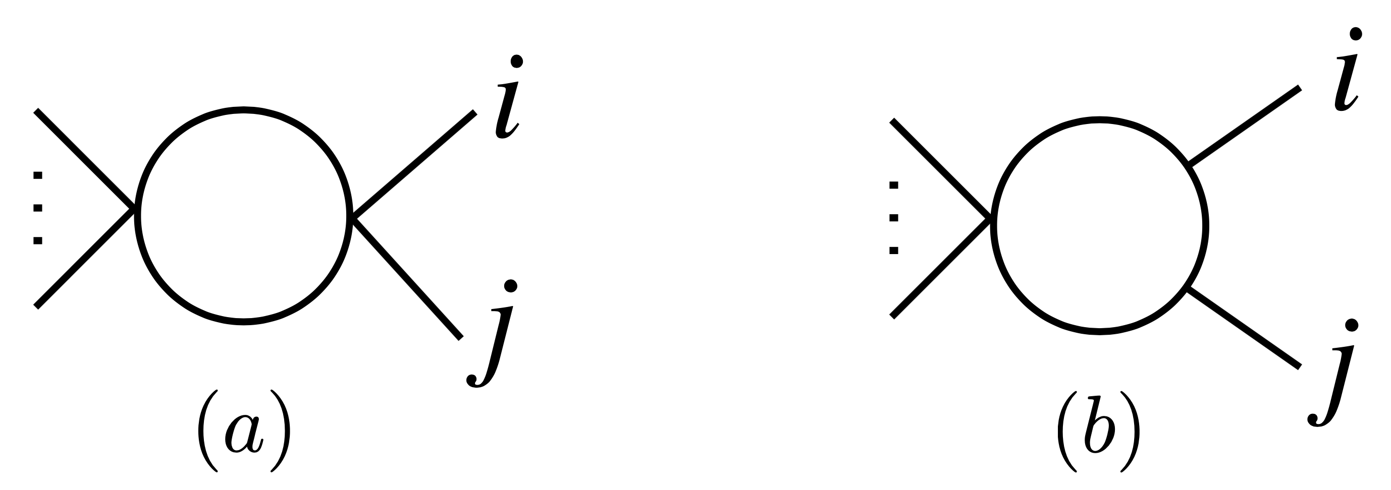
Figure 1: Bubble (a) and triangle (b) topologies which appear in the PV decomposition of $\mathcal{A}_{\rm loop}^{\rm IR}$ in gauge and gravity theories.

To treat the case in which IR divergencies are present, we need to know the explicit form of $\mathcal{A}_{\rm loop}^{\rm IR}$. For definiteness, we first consider gauge theories, and comment later on the case of gravity. By expanding the one-loop expressions given in [20, 21] on the PV basis, we find nonzero bubble coefficients related to collinear IR divergencies:

$$\hat{C}_{2}^{(ij)}=-8\pi^{2}\,\gamma_{\rm coll}^{(i)}\,\frac{{\bm{T}}_{i}\cdot{\bm{T}}_{j}}{{\bm{T}}_{i}^{2}}{\cal A}_{\rm tree}+(i\leftrightarrow j)\,,$$ (64)

where the external legs $i$ and $j$ are as shown in Fig. 1 ($a$), and we follow the color-space notation usually adopted, with color/flavor indices left implicit [20, 21]. When we unfold them, we have

$${\cal A}_{\rm tree}\to{\cal A}_{\rm tree}^{abcd}\ \ {\rm and}\ \ {\bm{T}}_{i}\to(T_{i}^{A})_{a}^{a^{\prime}}\,,$$ (65)

where the generator $T_{i}$ is in the representation appropriate for particle $i$. The dot-product is ${\bm{T}}_{i}\cdot{\bm{T}}_{j}\equiv{\bm{T}}_{i}^{A}{\bm{T}}_{j}^{A}$ (see e.g. [20] for more details). We then sum over all ${\rm cut}^{(ij)}$ with $i<j$, where the indices $i,j$ label the two legs that are cut out from the rest of the states. The bubble contributions then reduce to a sum over particle legs:

$$-\sum_{i<j}{\rm cut}^{(ij)}\left[\mathcal{A}_{\rm loop}^{\rm IR}\right]|_{\rm bubble}=\frac{1}{8\pi^{2}}\sum_{i<j}\hat{C}_{2}^{(ij)}=\sum_{i}\gamma_{\rm coll}^{(i)}{\cal A}_{\rm tree}=\gamma_{\rm coll}{\cal A}_{\rm tree}\,,$$ (66)

thanks to the property of color/flavor conservation, $\sum_{j}{\bm{T}}_{j}{\cal A}_{\rm tree}=0$. This reproduces Eq. (18).

On the other hand, soft IR divergencies give contributions to 1-mass triangles, with coefficients

$$\hat{C}_{3}^{(ij)}=-g^{2}s_{ij}\,{\bm{T}}_{i}\cdot{\bm{T}}_{j}\,{\cal A}_{\rm tree}\,,$$ (67)

where $i$ and $j$ label the external legs, as shown in Fig. 1 ($b$). In this case, a 2-cut gives

$${\rm cut}^{(ij)}\left[\mathcal{A}_{\rm loop}^{\rm IR}\right]|_{\rm triangle}=\hat{C}_{3}^{(ij)}{\rm cut}[I_{3}^{(ij)}]=\frac{1}{4\pi^{3}}\,g^{2}\,{\bm{T}}_{i}\cdot{\bm{T}}_{j}\,{\cal A}_{\rm tree}\int d{\rm LIPS}\,\frac{1}{s_{\theta^{\prime}\!/2}^{2}}\,.$$ (68)

In the last step, we could have equally well expressed the cut of the triangle as $\int{c_{\theta^{\prime}\!/2}^{-2}}$, which is the same after the substitution $\theta^{\prime}\to(\pi-\theta^{\prime})$, or as $2\int{s_{\theta^{\prime}}^{-2}}$, obtained by symmetrization over the interval $[0,\pi]$. We will use Eq. (68) when either ${\cal A}_{L}$ or ${\cal A}_{R}$ is singular for $\theta\to 0$. In this case we have ${\cal A}_{L,R}\sim s^{-2}_{\theta/2}$, and the integrand in Eq. (16) is well-behaved. When ${\cal A}_{L,R}\sim s^{-2}_{\theta}$, as it happens when the two incoming/outgoing particles are identical, we need to replace $\int s^{-2}_{\theta^{\prime}\!/2}$ in Eq. (68) by $2\int{s_{\theta^{\prime}}^{-2}}$, and similarly for Eq. (16).

Using Eq. (68) in Eq. (63), we obtain Eq. (15), with the identification ${\bm{T}}_{\rm soft}^{ij}=g^{2}\,{\bm{T}}_{i}\cdot{\bm{T}}_{j}$. Notice that in QED we simply have ${\bm{T}}_{\rm soft}^{ij}=e^{2}q_{i}q_{j}$. For gravity, IR divergencies have the same PV structure as for gauge theories, with $\gamma_{\rm coll}=0$ and ${\bm{T}}_{\rm soft}^{ij}=-2s_{ij}/M_{P}^{2}$ [22].

Soft singularities are also present in scalar amplitudes involving the exchange of a massless scalar. The methods discussed here and in Sec. 2.3 can be easily extended to this case. Instead, 4-point amplitudes involving Yukawa interactions never feature $\theta\to 0$ singularities, as they go at worst like $\theta^{-1}$ (and the same for $\theta\to\pi$).

Appendix B Partial-wave decomposition

Let us consider the process $1,2\to 3,4$, where the incoming pair $1,2$ lies in the direction defined by the polar angles $(\psi,\omega)$ and the outgoing pair $3,4$ in the direction defined by the angles $(\theta,\phi)$. By using the completeness of the angular momentum basis, the amplitude can be written as

$${\cal A}(s,\theta,\phi;\psi,\omega)\equiv\langle\theta\phi;h_{3}h_{4}|\mathcal{T}|\psi\omega;h_{1}h_{2}\rangle$$ (69)

$$= \sum_{JJ^{\prime}MM^{\prime}}\langle\theta\phi;h_{3}h_{4}|J^{\prime}M^{\prime};h_{3}h_{4}\rangle\langle J^{\prime}M^{\prime};h_{3}h_{4}|\mathcal{T}|JM;h_{1}h_{2}\rangle\langle JM;h_{1}h_{2}|\psi\omega;h_{1}h_{2}\rangle\,.$$

Due to angular momentum conservation, we have

$$\langle J^{\prime}M^{\prime};h_{3}h_{4}|\mathcal{T}|JM;h_{1}h_{2}\rangle=\delta_{MM^{\prime}}\,\delta_{JJ^{\prime}}\left(\frac{\sqrt{s}}{\Lambda}\right)^{w}a^{J}.$$ (70)

Applied to Eq. (69), this gives

$${\cal A}(s,\theta,\phi;\psi,\omega)=\left(\frac{\sqrt{s}}{\Lambda}\right)^{w}\sum_{JM}n_{J}\,e^{i\phi(M-h_{34})}d_{Mh_{34}}^{J}(\theta)\,e^{-i\omega(M-h_{12})}d_{Mh_{12}}^{J}(\psi)\,a^{J},$$ (71)

where we have defined $n_{J}=2J+1$ and have introduced the Wigner $d$-functions

$${d}^{J}_{Mh_{12}}(\theta)=\frac{e^{i\phi(M-h_{12})}}{\sqrt{n_{J}}}\langle JM;h_{1}h_{2}|\theta\phi;h_{1}h_{2}\rangle\,.$$ (72)

They can be expressed in terms of trigonometric functions as

$${d}^{J}_{MM^{\prime}}(\theta)=\Bigl{[}(J+M)!\,(J-M)!\,(J+M^{\prime})!\,(J-M^{\prime})!\Bigr{]}^{1/2}\\ \times\sum_{S}\left[\frac{(-1)^{M^{\prime}-M+S}\,c_{\theta/2}^{~{}2J+M-M^{\prime}-2S}\,s_{\theta/2}^{~{}M^{\prime}-M+2S}}{(J+M-S)!\,S!\,(M^{\prime}-M+S)!\,(J-M^{\prime}-S)!}\right],$$ (73)

where the sum is over all $S$ such that the arguments of the factorials in the denominator are nonnegative. The Wigner $d$-functions fulfil an orthogonality condition given by

$$\int_{0}^{\pi}d\theta\,s_{\theta}\,d_{MM^{\prime}}^{J}(\theta)d_{MM^{\prime}}^{J^{\prime}}(\theta)=\frac{2\delta_{JJ^{\prime}}}{n_{J}}.$$ (74)

We always have the freedom to choose a frame such that $\psi=\omega=0$, giving

$${\cal A}(s,\theta,\phi)=e^{i\phi(h_{12}-h_{34})}\left(\frac{\sqrt{s}}{\Lambda}\right)^{w}\sum_{J}n_{J}\,d_{h_{12}h_{34}}^{J}(\theta)\,a^{J},$$ (75)

where we have used the property $d^{J}_{MM^{\prime}}(0)=\delta_{MM^{\prime}}$.

References

- [1] Z. Bern, J. Parra-Martinez and E. Sawyer, Phys. Rev. Lett. 124 (2020) no.5, 051601 [arXiv:1910.05831 [hep-ph]].
- [2] J. Elias Miró, J. Ingoldby and M. Riembau, JHEP 09 (2020), 163 [arXiv:2005.06983 [hep-ph]].
- [3] P. Baratella, C. Fernandez and A. Pomarol, Nucl. Phys. B (2020), 115155 [arXiv:2005.07129 [hep-ph]].
- [4] Z. Bern, J. Parra-Martinez and E. Sawyer, [arXiv:2005.12917 [hep-ph]].
- [5] M. Jiang, T. Ma and J. Shu, [arXiv:2005.10261 [hep-ph]].
- [6] N. Arkani-Hamed, F. Cachazo and J. Kaplan, JHEP 1009 (2010) 016 [arXiv:0808.1446 [hep-th]].
- [7] Y. -t. Huang, D. A. McGady and C. Peng, Phys. Rev. D 87 (2013) no.8, 085028 [arXiv:1205.5606 [hep-th]].
- [8] S. Caron-Huot and M. Wilhelm, JHEP 1612 (2016) 010 [arXiv:1607.06448 [hep-th]].
- [9] Z. Bern, H. H. Chi, L. Dixon and A. Edison, Phys. Rev. D 95 (2017) no.4, 046013 [arXiv:1701.02422 [hep-th]].
- [10] M. Jiang, J. Shu, M. L. Xiao and Y. H. Zheng, [arXiv:2001.04481 [hep-ph]].
- [11] M. Jacob and G. C. Wick, Annals Phys. 7 (1959), 404-428.
- [12] L. J. Dixon, arXiv:1310.5353 [hep-ph].
- [13] Y. Shadmi and Y. Weiss, JHEP 02 (2019), 165 [arXiv:1809.09644 [hep-ph]]; T. Ma, J. Shu and M. L. Xiao, [arXiv:1902.06752 [hep-ph]]; R. Aoude and C. S. Machado, JHEP 12 (2019), 058 [arXiv:1905.11433 [hep-ph]]; G. Durieux, T. Kitahara, Y. Shadmi and Y. Weiss, JHEP 01 (2020), 119 [arXiv:1909.10551 [hep-ph]]; G. Durieux and C. S. Machado, [arXiv:1912.08827 [hep-ph]];
- [14] S. L. Adler, Phys. Rev. 137 (1965) B1022.
- [15] L. Susskind and G. Frye, Phys. Rev. D 1 (1970), 1682-1686.
- [16] I. Low and Z. Yin, JHEP 1911 (2019) 078 [arXiv:1904.12859 [hep-th]]; L. Dai, I. Low, T. Mehen and A. Mohapatra, [arXiv:2009.01819 [hep-ph]].
- [17] K. Kampf, J. Novotny and J. Trnka, JHEP 05 (2013), 032 [arXiv:1304.3048 [hep-th]].
- [18] J. Bijnens, G. Colangelo, G. Ecker, J. Gasser and M. E. Sainio, Phys. Lett. B 374 (1996), 210-216 [arXiv:hep-ph/9511397 [hep-ph]].
- [19] P. Baratella, “Aspects of Chiral Perturbation Theory from an on-shell perspective”, talk at COST Workshop: Probing BSM physics at different scales , Berlin, January 2020.
- [20] S. Catani, Phys. Lett. B 427 (1998), 161-171 [arXiv:hep-ph/9802439 [hep-ph]].
- [21] T. Becher and M. Neubert, Phys. Rev. Lett. 102 (2009), 162001 [arXiv:0901.0722 [hep-ph]].
- [22] D. C. Dunbar and P. S. Norridge, Class. Quant. Grav. 14 (1997), 351-365 [arXiv:hep-th/9512084 [hep-th]].