Covariate-adjusted Fisher randomization tests for the average treatment effect

Abstract

Fisher’s randomization test (frt) delivers exact $p$-values under the strong null hypothesis of no treatment effect on any units whatsoever and allows for flexible covariate adjustment to improve the power. Of interest is whether the resulting covariate-adjusted procedure could also be valid for testing the weak null hypothesis of zero average treatment effect. To this end, we evaluate two general strategies for conducting covariate adjustment in frts: the “pseudo-outcome” strategy that uses the residuals from an outcome model with only the covariates as the pseudo, covariate-adjusted outcomes to form the test statistic, and the “model-output” strategy that directly uses the output from an outcome model with both the treatment and covariates as the covariate-adjusted test statistic. Based on theory and simulation, we recommend using the ordinary least squares (ols) fit of the observed outcome on the treatment, centered covariates, and their interactions for covariate adjustment, and conducting frt with the robust $t$-value of the treatment as the test statistic. The resulting frt is finite-sample exact for testing the strong null hypothesis, asymptotically valid for testing the weak null hypothesis, and more powerful than the unadjusted counterpart under alternatives, all irrespective of whether the linear model is correctly specified or not. We start with complete randomization, and then extend the theory to cluster randomization, stratified randomization, and rerandomization, respectively, giving a recommendation for the test procedure and test statistic under each design. Our theory is design-based, also known as randomization-based, in which we condition on the potential outcomes but average over the random treatment assignment.

Keywords: Finite-population inference; permutation test; randomization distribution; robust standard error; studentization; super-population inference

Fisher’s randomization test with covariate adjustment

Fisher (1935) viewed randomization as a “reasoned basis” for inference and proposed the randomization test as a universal way to generate finite-sample exact $p$-values without imposing modeling assumptions on the experimental outcomes. Fisher’s randomization test (frt) becomes increasingly important with the popularity of field experiments in social sciences in addition to the traditional biomedical experiments. Proschan and Dodd (2019) reviewed the use of frts in randomized clinical trials and highlighted its strength in analyzing complex data. There is an increasing interest in economics and related fields to use frts to analyze various types of empirical data (Freedman and Lane 1983; Kennedy 1995; Lee and Shaikh 2014; Cattaneo et al. 2015; Canay et al. 2017; Ganong and Jäger 2018; Athey et al. 2018; Bugni et al. 2018; Young 2019; Heckman and Karapakula 2021; MacKinnon and Webb 2020; Heckman et al. 2020).

The flexibility of frt enables two natural strategies to incorporate covariate information via statistical modeling. First, we can fit a statistical model of the outcome on the covariates to obtain the residuals as the covariate-adjusted pseudo outcomes, and proceed with the usual frt in a covariate-free fashion. Tukey (1993) used it with linear models, Gail et al. (1988) used it with generalized linear models, Raz (1990) used it with nonparametric regressions, Stephens et al. (2013) used it with the generalized estimating equation for clustered data, and Rosenbaum (2002) reviewed and extended it to not only randomized experiments but also matched observational studies. Second, we can directly fit an outcome model with both the treatment and covariates, and use the model output, such as the coefficient of the treatment or the corresponding $t$-value, as the test statistic. The canonical choice is a linear model on the treatment and covariates, often known as the analysis of covariance (Fisher 1935; Freedman 2008; Lin 2013; Young 2019). Brillinger et al. (1978) gave an early application of this strategy with more complex statistical models. This defines two model-assisted approaches to conducting covariate-adjusted frts.

The strong guarantees of frt hold only under the strong null hypothesis of zero individual treatment effects, which is often criticized for being too restrictive for many practical applications. Adaptation to the weak null hypothesis of zero average treatment effect is one important direction for broadening its application. A natural class of test statistics for this purpose are the coefficients of the treatment from various outcome models, with or without covariate adjustment, along with their classic or robustly-studentized $t$-statistics (Eicker 1967; Huber 1967; White 1980). These coefficients are consistent estimators of the average treatment effect and are thus sensitive to deviations from both the strong and weak null hypotheses (Freedman 2008; Lin 2013). Of interest is whether these intuitive test statistics can preserve the correct type one error rates when only the weak null hypothesis holds (Romano 1990; Chung and Romano 2013; Wu and Ding 2020), and if covariate adjustment delivers additional power under alternatives.

To this end, we extend the discussion by Ding and Dasgupta (2018) and Wu and Ding (2020) on the utility of frt for testing the weak null hypothesis to the presence of covariates under the finite-population framework, and examine the asymptotic operating characteristics of nine covariate-adjusted test statistics as the coefficients from three common outcome models and their respective classic and robustly-studentized $t$-statistics. The results establish the permutational limiting theorems of the ols coefficients and standard errors under the possibly misspecified linear models, and shed light on the utility of model-assisted covariate adjustment for testing the weak null hypothesis via frt. Building upon previous work on using studentized statistics for permutation tests under the super-population (Janssen 1997; Chung and Romano 2013; Pauly et al. 2015; Bugni et al. 2018) and finite-population (Wu and Ding 2020) frameworks, respectively, we extend the discussion to the covariate-adjusted test statistics under the finite-population framework, and show the necessity of robust studentization for ensuring the asymptotic validity of the covariate-adjusted test statistics when only the weak null hypothesis holds. The robustly studentized $t$-statistic based on Lin (2013)’s estimator, as it turns out, guarantees both asymptotic validity and the highest power for testing the weak null hypothesis. The estimator equals the coefficient of the treatment in the ols fit of the outcome on the treatment, centered covariates, and their interactions, but the aforementioned theoretical guarantees hold irrespective of whether the linear model is correctly specified or not. Together with its finite-sample exactness under the strong null hypothesis, it is thus our final recommendation for testing both the strong and weak null hypotheses under complete randomization.

We first focus on complete randomization and then generalize the theory to other types of design. The extension to cluster randomization and stratified randomization is direct whereas that to rerandomization (Morgan and Rubin 2012) has some distinct features. In particular, covariate adjustment becomes more crucial since studentization alone no longer ensures the appropriateness of frt for the weak null hypothesis. In addition, it is common that the designer and analyzer do not communicate (Bruhn and McKenzie 2009; Heckman et al. 2020; Heckman and Karapakula 2021), and if this happens, we recommend using frt pretending that the experiment was completely randomized. In this non-ideal case, the proposed frt is no longer finite-sample exact under the strong null hypothesis unless the original experiment is indeed completely randomized, but at least it preserves the correct type one error rates under the weak null hypothesis. Based on extensive theoretical investigations, we make final recommendations for frt and the test statistic in each experimental design.

We will use the following notation for permutations. Let $\Pi$ be the set of all $N!$ random permutations of $\{1,\dots,N\}$, indexed by $\pi$. For an $N\times 1$ vector $a=(a_{1},\dots,a_{N})^{\mathrm{\scriptscriptstyle T}}$, let $a_{\pi}=(a_{\pi(1)},\dots,a_{\pi(N)})^{\mathrm{\scriptscriptstyle T}}$ be a permutation of its elements. If $b=b(a)$ is a function of $a$, let $b^{\pi}=b(a_{\pi})$ be its value evaluated at $a_{\pi}$. Without introducing new notation, use $\pi$ to also represent a random draw from $\Pi$, namely $\pi\sim\operatorname{Unif}(\Pi)$, with meaning clear from the context. With a slight abuse of notation, assume sets like $\{a_{\pi}:\pi\in\Pi\}$ to contain $|\Pi|=N!$ elements defined by $\pi\in\Pi$ throughout, such that $a_{\pi}$ and $a_{\pi^{\prime}}$ are two distinct elements so long as $\pi\neq\pi^{\prime}$, even if $a_{\pi}=a_{\pi^{\prime}}$.

Basic setup under complete randomization

2.1 Potential outcomes and Fisher’s randomization test

Consider an intervention of two levels, $z=0,1$, and a finite population of $N$ units, $i=1,\ldots,N$. Let $Y_{i}(z)$ be the potential outcome of unit $i$ under treatment $z$ (Neyman 1923/1990). The individual treatment effect is $\tau_{i}=Y_{i}(1)-Y_{i}(0)$, and the finite-population average treatment effect is $\tau=N^{-1}\sum_{i=1}^{N}\tau_{i}$. We focus on the finite-population inference in the main text, and will refer to $\tau$ as the “average treatment effect” when no confusion would arise. Let $x_{i}=(x_{i1},\ldots,x_{iJ})^{\mathrm{\scriptscriptstyle T}}$ be the covariates for unit $i$, concatenated as an $N\times J$ matrix $X=(x_{1},\dots,x_{N})^{\mathrm{\scriptscriptstyle T}}$. Center the covariates at $\bar{x}=N^{-1}\sum_{i=1}^{N}x_{i}=0_{J}$ to simplify the presentation.

The designer assigns $N_{z}$ units to receive level $z$ with $N_{1}+N_{0}=N$ and $(p_{1},p_{0})=(N_{1}/N,N_{0}/N).$ Let $Z_{i}$ denote the treatment level received by unit $i$, with $Z_{i}=1$ for treatment and $Z_{i}=0$ for control, vectorized as $Z=(Z_{1},\dots,Z_{N})^{\mathrm{\scriptscriptstyle T}}$. Complete randomization samples $Z$ uniformly from the set $\mathcal{Z}$ that contains all permutations of $N_{1}$ 1’s and $N_{0}$ 0’s. The observed outcome is $Y_{i}=Z_{i}Y_{i}(1)+(1-Z_{i})Y_{i}(0)$ for unit $i$, vectorized as $Y=(Y_{1},\ldots,Y_{N})^{\mathrm{\scriptscriptstyle T}}$. A test statistic is a function of the treatment vector, observed outcomes, and covariates, denoted by $T=T(Z,Y,X)$.

Write $Y=Y(Z)$ and $T=T(Z,Y(Z),X)$ to highlight the dependence of the observed outcomes and the test statistic on the treatment vector. Complete randomization induces a uniform distribution over $\{T(\bm{z},Y(\bm{z}),X):\bm{z}\in\mathcal{Z}\}$ as the sampling distribution of $T$. Fisher (1935) considered testing the strong null hypothesis

$$H_{0{\textsc{f}}}:Y_{i}(1)=Y_{i}(0)\quad\text{for all $i=1,\ldots,N$}$$

and proposed frt to compute the $p$-value as

$$p_{\textsc{frt}}=|\Pi|^{-1}\sum_{\pi\in\Pi}1\{T(Z_{\pi},Y,X)\geq T(Z,Y,X)\},$$ (1)

assuming a one-sided test. Each $Z_{\pi}$ is a permutation of $Z$, and by symmetry, all possible values of $Z_{\pi}$ over $\pi\in\Pi$ consist of $\mathcal{Z}$. frt thus induces a uniform distribution over $\{T(\bm{z},Y(Z),X):\bm{z}\in\mathcal{Z}\}$ conditioning on the observed $Z$, known as the randomization distribution of $T$. Let $T^{\pi}=T(Z_{\pi},Y(Z),X)$, where $\pi\sim\operatorname{Unif}(\Pi)$, be a random variable from this distribution conditioning on $Z$. The $p_{\textsc{frt}}$ in (1) gives the right-tail probability of the observed value of the test statistic with regard to its randomization distribution. Under $H_{0{\textsc{f}}}$, the randomization distribution equals the sampling distribution, and thereby ensures the finite-sample exactness of frt for arbitrary $T$.

In practice, we need to choose a test statistic that is sensitive to deviations from $H_{0{\textsc{f}}}$. Computationally, frt involves randomly permuting the treatment vector to generate $Z_{\pi}$. This justifies “permutation test” as its other name. If $|\Pi|=N!$ is too large, we can take a simple random sample from $\Pi$ to obtain a Monte Carlo approximation of $p_{\textsc{frt}}$.

Remark 1.

Based on the definition in (1), frt does not require any algebraic group structure of the treatment assignment mechanism. Therefore, it is more general than the usual definition of permutation test which requires certain invariance under group transformations (Hoeffding 1952; Lehmann and Romano 2005). Nevertheless, we will focus on frts that can be implemented by permutations or restricted permutations in this paper. See Basse et al. (2019) for more discussion on the connections and distinctions.

The nice properties of frt under $H_{0{\textsc{f}}}$ inspire endeavors to extend it to other types of hypotheses. Consider the weak null hypothesis of zero average treatment effect (Neyman 1935):

$$H_{0{\textsc{n}}}:\tau=0.$$

We can proceed with frt by permuting the treatment vector $Z$ and report $p_{\textsc{frt}}$ by (1) as if we were testing $H_{0{\textsc{f}}}$. Under $H_{0{\textsc{n}}}$, $Y(\bm{z})$ varies with $\bm{z}\in\mathcal{Z}$ such that the randomization distribution $T^{\pi}$ no longer equals the sampling distribution $T$. Consequently, $p_{\textsc{frt}}$ loses its finite-sample exactness as the basis for controlling the type one error rates in general. Wu and Ding (2020) gave examples in which frt yields invalid type one error rates under $H_{0{\textsc{n}}}$ even asymptotically.

The discrepancy between the distributions of $T$ and $T^{\pi}$ in the absence of $H_{0{\textsc{f}}}$ is at the heart of the loss of finite-sample exactness when applying frt to hypotheses other than $H_{0{\textsc{f}}}$. The sampling distribution of $T$, on the one hand, is induced by the randomization of $Z$ based on the “true finite population” of $\{(Y_{i}(0),Y_{i}(1),x_{i}\}_{i=1}^{N}$. The frt procedure, on the other hand, assumes the observed outcomes $Y=(Y_{1},\dots,Y_{N})^{\mathrm{\scriptscriptstyle T}}$ remain unchanged over all possible assignments, and is essentially using $\{(Y_{i}^{\prime}(0),Y_{i}^{\prime}(1),x_{i}\}_{i=1}^{N}$, where $Y_{i}^{\prime}(0)=Y_{i}^{\prime}(1)=Y_{i}$, as the “pseudo finite population” to generate the randomization distribution of $T$, represented by $T^{\pi}$. This ends up mixing $\{Y_{i}(0)\}_{i=1}^{N}$ and $\{Y_{i}(1)\}_{i=1}^{N}$ with proportions $p_{0}$ and $p_{1}$ in the absence of $H_{0{\textsc{f}}}$, and thereby results in the different distributions of $T$ and $T^{\pi}$.

Despite the possibly liberal type one error rates in general, sensible choice of the test statistic restores the validity of frt for testing $H_{0{\textsc{n}}}$ at least asymptotically. Wu and Ding (2020) showed that frt preserves the correct type one error rates asymptotically with a class of robustly studentized statistics. We extend their discussion to the setting with covariates, and propose a general strategy for covariate-adjusted frt that ensures both asymptotic validity and higher power for testing $H_{0{\textsc{n}}}$.

Assume the finite-population asymptotic framework that embeds $\mathcal{S}=\{Y_{i}(0),Y_{i}(1),x_{i}\}_{i=1}^{N}$ and $Z=(Z_{i})_{i=1}^{N}$ into a sequence of finite populations and assignments for $N=1,\ldots,\infty$. Technically, all quantities depend on $N$, but we omit the subscript $N$ for simplicity.

Definition 1.

A test statistic $T$ is proper for testing $H_{0{\textsc{n}}}$ if under $H_{0{\textsc{n}}}$,

$$\lim_{N\to\infty}{\rm pr}(p_{\textsc{frt}}\leq\alpha)\leq\alpha\qquad\text{for all }\alpha\in(0,1)$$

holds for any $\mathcal{S}$.

Assume a one-sided test and $p$-value as the right-tail probability as in (1). A statistic $T$ is proper for testing $H_{0{\textsc{n}}}$ if under $H_{0{\textsc{n}}}$, the sampling distribution of $T$ is stochastically dominated by its randomization distribution for almost all sequences of $Z$ as $N\to\infty$.

2.2 Two strategies for covariate-adjusted FRT and twelve test statistics

We review two general strategies for covariate adjustment in frt. We focus on test statistics based on estimators of $\tau$ to accommodate both $H_{0{\textsc{f}}}$ and $H_{0{\textsc{n}}}$, and unify them under the ols formulation for easy implementation.

Let $\hat{Y}(z)=N_{z}^{-1}\sum_{i:Z_{i}=z}Y_{i}$ be the sample average of the outcomes under treatment $z$. The difference-in-means estimator $\hat{\tau}_{\textsc{n}}=\hat{Y}(1)-\hat{Y}(0)$ is unbiased for $\tau$ under complete randomization (Neyman 1923/1990), and affords a natural statistic for testing both $H_{0{\textsc{f}}}$ and $H_{0{\textsc{n}}}$. Algebraically, it equals the coefficient of $Z_{i}$ from the ols fit of $Y_{i}$ on $(1,Z_{i})$. It is also common to use $\hat{\tau}_{\textsc{n}}/{\hat{\textup{se}}_{\textsc{n}}}$ or $\hat{\tau}_{\textsc{n}}/\tilde{\textup{se}}_{\textsc{n}}$ as the test statistic, where ${\hat{\textup{se}}_{\textsc{n}}}$ and $\tilde{\textup{se}}_{\textsc{n}}$ are the classic and robust standard errors from the same ols fit:

$$\hat{\textup{se}}_{\textsc{n}}^{2}=\frac{N(N_{1}-1)}{(N-2)N_{1}N_{0}}\hat{S}_{1}^{2}+\frac{N(N_{0}-1)}{(N-2)N_{1}N_{0}}\hat{S}_{0}^{2}\approx\frac{\hat{S}_{1}^{2}}{N_{0}}+\frac{\hat{S}_{0}^{2}}{N_{1}},\quad\tilde{\textup{se}}_{\textsc{n}}^{2}=\frac{N_{1}-1}{N_{1}^{2}}\hat{S}_{1}^{2}+\frac{N_{0}-1}{N_{0}^{2}}\hat{S}_{0}^{2}\approx\frac{\hat{S}_{1}^{2}}{N_{1}}+\frac{\hat{S}_{0}^{2}}{N_{0}}$$

with $\hat{S}_{z}^{2}=(N_{z}-1)^{-1}\sum_{i:Z_{i}=z}\{Y_{i}-\hat{Y}(z)\}^{2}\ (z=0,1)$ (Angrist and Pischke 2009). This yields three unadjusted test statistics as the baseline for discussing the possible improvement via covariate adjustment. The randomization distributions can then be generated by replacing $Z_{i}$ with $Z_{\pi(i)}$ in the above ols fit over all $\pi\in\Pi$. In particular, we can compute $\hat{\tau}_{\textsc{n}}^{\pi}$ as the coefficient of $Z_{\pi(i)}$ from the ols fit of $Y_{i}$ on $(1,Z_{\pi(i)})$ with $(\hat{\tau}_{\textsc{n}}/\hat{\textup{se}}_{\textsc{n}})^{\pi}=\hat{\tau}_{\textsc{n}}^{\pi}/{\hat{\textup{se}}_{\textsc{n}}^{\pi}}$ and $(\hat{\tau}_{\textsc{n}}/\tilde{\textup{se}}_{\textsc{n}})^{\pi}=\hat{\tau}_{\textsc{n}}^{\pi}/{\tilde{\textup{se}}_{\textsc{n}}^{\pi}}$, where ${\tilde{\textup{se}}_{\textsc{n}}^{\pi}}$ and ${\hat{\textup{se}}_{\textsc{n}}^{\pi}}$ are the corresponding classic and robust standard errors. The same intuition extends to the covariate-adjusted variants below as we shall introduce in a minute. Chung and Romano (2013) and Wu and Ding (2020) showed that randomization tests with the robustly studentized $\hat{\tau}_{\textsc{n}}/\tilde{\textup{se}}_{\textsc{n}}$ are asymptotically valid for $H_{0{\textsc{n}}}$ under the super- and finite-population frameworks, respectively. We thus also consider studentization in covariate adjustment.

The first strategy for covariate adjustment is to fit an outcome model with covariates alone and use the residuals as the fixed, covariate-adjusted pseudo outcomes for conducting frt. This appears to be the dominating approach advocated by Rosenbaum (2002); see also Gail et al. (1988), Raz (1990), Tukey (1993) and Ottoboni et al. (2018). Let $e=(e_{1},\dots,e_{N})^{\mathrm{\scriptscriptstyle T}}$ be the residuals from the ols fit of $Y_{i}$ on $(1,x_{i})$, which can be viewed as pseudo outcomes unaffected by the treatment under $H_{0{\textsc{f}}}$. The difference in means of the residuals, $\hat{\tau}_{\textsc{r}}=\hat{e}(1)-\hat{e}(0)$, equals the coefficient of $Z_{i}$ from the ols fit of $e_{i}$ on $(1,Z_{i})$ and affords an intuitive estimator of $\tau$ after adjusting for the covariates. Similar to the discussion of $\hat{\tau}_{\textsc{n}}$, we can use $\hat{\tau}_{\textsc{r}}$, $\hat{\tau}_{\textsc{r}}/\hat{\textup{se}}_{\textsc{r}}$, and $\hat{\tau}_{\textsc{r}}/\tilde{\textup{se}}_{\textsc{r}}$ as the test statistics for testing $H_{0{\textsc{f}}}$ or $H_{0{\textsc{n}}}$ by frt, where $\hat{\textup{se}}_{\textsc{r}}$ and $\tilde{\textup{se}}_{\textsc{r}}$ are the classic and robust standard errors from the ols fit that yields $\hat{\tau}_{\textsc{r}}$. We regress $Y_{i}$ on $(1,x_{i})$ to form the residuals $e$ whereas Rosenbaum (2002) regressed $Y_{i}$ on $x_{i}$ alone without the intercept. The difference does not affect $\hat{\tau}_{\textsc{r}}$ with centered covariates.

The second strategy for covariate adjustment is to directly fit an outcome model with both the treatment and covariates, and use the coefficient or $t$-values of the treatment as the test statistic for frt. Fisher (1935) suggested an estimator $\hat{\tau}_{\textsc{f}}$ for $\tau$, which equals the coefficient of $Z_{i}$ from the ols fit of $Y_{i}$ on $(1,Z_{i},x_{i})$. Lin (2013) recommended an improved estimator, $\hat{\tau}_{\textsc{l}}$, as the coefficient of $Z_{i}$ from the ols fit of $Y_{i}$ on $\{1,Z_{i},x_{i}-\bar{x},Z_{i}(x_{i}-\bar{x})\}$ with centered covariates and treatment-covariates interactions. These two covariate-adjusted estimators, along with their respective studentized variants, afford six additional test statistics, namely $\hat{\tau}_{*}$, $\hat{\tau}_{*}/\hat{\textup{se}}_{*}$, and $\hat{\tau}_{*}/\tilde{\textup{se}}_{*}\ (*={\textsc{f}},{\textsc{l}})$, for testing $H_{0{\textsc{f}}}$ or $H_{0{\textsc{n}}}$ by frt, where $\hat{\textup{se}}_{*}$ and $\tilde{\textup{se}}_{*}$ are the classic and robust standard errors from the respective ols fits.

Table 1: Twelve test statistics where $\hat{\textup{se}}$ and $\tilde{\textup{se}}$ denote the classic and robust standard errors.

	Neyman (1923/1990)	Rosenbaum (2002)	Fisher (1935)	Lin (2013)
unstudentized	$\hat{\tau}_{\textsc{n}}$	$\hat{\tau}_{\textsc{r}}$	$\hat{\tau}_{\textsc{f}}$	$\hat{\tau}_{\textsc{l}}$
studentized by $\hat{\textup{se}}$	$\hat{\tau}_{\textsc{n}}/{\hat{\textup{se}}_{\textsc{n}}}$	$\hat{\tau}_{\textsc{r}}/\hat{\textup{se}}_{\textsc{r}}$	$\hat{\tau}_{\textsc{f}}/\hat{\textup{se}}_{\textsc{f}}$	$\hat{\tau}_{\textsc{l}}/\hat{\textup{se}}_{\textsc{l}}$
studentized by $\tilde{\textup{se}}$	$\hat{\tau}_{\textsc{n}}/\tilde{\textup{se}}_{\textsc{n}}$	$\hat{\tau}_{\textsc{r}}/\tilde{\textup{se}}_{\textsc{r}}$	$\hat{\tau}_{\textsc{f}}/\tilde{\textup{se}}_{\textsc{f}}$	$\hat{\tau}_{\textsc{l}}/\tilde{\textup{se}}_{\textsc{l}}$

This gives us a total of twelve test statistics, three unadjusted and nine adjusted, for testing the treatment effects via frt. Table 1 summarizes them, with the subscripts n, r, f, and l indicating Neyman (1923/1990), Rosenbaum (2002), Fisher (1935), and Lin (2013), respectively. All twelve statistics are finite-sample exact for testing $H_{0{\textsc{f}}}$ irrespective of whether the models are correctly specified or not. Our goal is to evaluate their abilities to preserve the correct type one error rates under $H_{0{\textsc{n}}}$. Without loss of generality, we assume two-sided frt for the rest of the text, or, equivalently, we use the absolute values of the test statistics in Table 1 to compute the $p_{\textsc{frt}}$ in (1).

The two strategies for covariate adjustment unify nicely under the ols formulation yet differ materially with regard to the role of covariates under the permutations induced by the frt procedure. The first strategy, on the one hand, adjusts for the covariates only once to form the pseudo outcomes $e$ and proceeds with the permutations in a covariate-free fashion. The second strategy, on the other hand, adjusts for the covariates in each of the $N!$ permutations of $Z$.

Before giving the formal results on the finite-population asymptotics, we unify below the three covariate-adjusted estimators as the differences in means of distinct adjusted outcomes. Let $S_{x}^{2}=(N-1)^{-1}\sum_{i=1}^{N}x_{i}x_{i}^{\mathrm{\scriptscriptstyle T}}$ and $\hat{S}_{xY}=(N-1)^{-1}\sum_{i=1}^{N}x_{i}Y_{i}$ be the finite-population covariance matrices of the centered $(x_{i})_{i=1}^{N}$ with itself and $(Y_{i})_{i=1}^{N}$, respectively. Let $\hat{\tau}_{x}=\hat{x}(1)-\hat{x}(0)$ be the difference in means of the covariates under treatment and control, where $\hat{x}(z)=N_{z}^{-1}\sum_{i:Z_{i}=z}x_{i}$. Let $\hat{S}_{x(z)}^{2}=(N_{z}-1)^{-1}\sum_{i:Z_{i}=z}\{x_{i}-\hat{x}(z)\}\{x_{i}-\hat{x}(z)\}^{\mathrm{\scriptscriptstyle T}}$ and $\hat{S}_{xY(z)}=(N_{z}-1)^{-1}\sum_{i:Z_{i}=z}\{x_{i}-\hat{x}(z)\}\{Y_{i}-\hat{Y}(z)\}$ be the sample covariance matrices of $x_{i}$ with itself and $Y_{i}$ under treatment $z$. Let $\hat{\gamma}_{\textsc{r}}$ and $\hat{\gamma}_{\textsc{f}}$ be the coefficients of $x_{i}$ from the ols fits of $Y_{i}$ on $(1,x_{i})$ and $(1,Z_{i},x_{i})$, respectively. Let $\hat{\gamma}_{\textsc{l}}=p_{0}\hat{\gamma}_{{\textsc{l}},1}+p_{1}\hat{\gamma}_{{\textsc{l}},0}$, where $\hat{\gamma}_{{\textsc{l}},z}$ is the coefficient of $x_{i}$ from the ols fit of $Y_{i}$ on $(1,x_{i})$ over the units under treatment $z$.

Proposition 1.

We have

$$\hat{\tau}_{*} = N^{-1}_{1}\sum_{i:Z_{i}=1}(Y_{i}-x_{i}^{\mathrm{\scriptscriptstyle T}}\hat{\gamma}_{*})-N^{-1}_{0}\sum_{i:Z_{i}=0}(Y_{i}-x_{i}^{\mathrm{\scriptscriptstyle T}}\hat{\gamma}_{*})=\hat{\tau}_{\textsc{n}}-\hat{\tau}_{x}^{\mathrm{\scriptscriptstyle T}}\hat{\gamma}_{*},\quad(*={\textsc{r}},{\textsc{f}})$$

$$\hat{\tau}_{\textsc{l}} = N^{-1}_{1}\sum_{i:Z_{i}=1}(Y_{i}-x_{i}^{\mathrm{\scriptscriptstyle T}}\hat{\gamma}_{{\textsc{l}},1})-N^{-1}_{0}\sum_{i:Z_{i}=0}(Y_{i}-x_{i}^{\mathrm{\scriptscriptstyle T}}\hat{\gamma}_{{\textsc{l}},0})=\hat{\tau}_{\textsc{n}}-\hat{\tau}_{x}^{\mathrm{\scriptscriptstyle T}}\hat{\gamma}_{\textsc{l}},$$

where $\hat{\gamma}_{\textsc{r}}=(S^{2}_{x})^{-1}\hat{S}_{xY}$, $\hat{\gamma}_{\textsc{f}}=\hat{\gamma}_{\textsc{r}}-(1-1/N)^{-1}p_{1}p_{0}\hat{\tau}_{\textsc{f}}(S_{x}^{2})^{-1}\hat{\tau}_{x}$, and $\hat{\gamma}_{{\textsc{l}},z}=(\hat{S}_{x(z)}^{2})^{-1}\hat{S}_{xY(z)}$.

Proposition 1 entails only the algebraic properties of the ols fits and holds under arbitrary data generating process. It unifies $\hat{\tau}_{*}\ (*={\textsc{r}},{\textsc{f}},{\textsc{l}})$ as the difference-in-means estimators defined on the adjusted outcomes, or, equivalently, as $\hat{\tau}_{\textsc{n}}$ with corrections based on the imbalance in means of the covariates.

Under $H_{0{\textsc{n}}}$, frt with $\hat{\tau}_{\textsc{n}}$ does not preserve the correct type one error rates but frt with $\hat{\tau}_{\textsc{n}}/\tilde{\textup{se}}_{\textsc{n}}$ does (Ding and Dasgupta 2018). In the next section, we will extend the result to the nine covariate-adjusted test statistics in Table 1 and establish the properness of the four robustly studentized $t$-statistics, namely $\hat{\tau}_{*}/\tilde{\textup{se}}_{*}\ (*={\textsc{n}},{\textsc{r}},{\textsc{f}},{\textsc{l}})$, for testing $H_{0{\textsc{n}}}$. Refer to them as the robust $t$-statistics hence. We will further show that among them, $\hat{\tau}_{\textsc{l}}/\tilde{\textup{se}}_{\textsc{l}}$ delivers the highest power under alternative hypotheses.

Remark 2.

Inspired by the distinction between $\hat{\tau}_{\textsc{f}}$ and $\hat{\tau}_{\textsc{l}}$ under the second covariate adjustment strategy, an alternative way to implement the first, pseudo-outcome-based strategy is to fit two separate ols regressions of $Y_{i}$ on $x_{i}$ for the treated and control units, respectively, both without the intercept, and then use the resulting residuals for conducting frt. Despite the computational advantage of this approach in that it adjusts for the covariates only once, the resulting tests lead to distinct sampling and randomization distributions even under $H_{0{\textsc{f}}}$, and are thus not finite-sample exact for testing $H_{0{\textsc{f}}}$. We see the finite-sample exactness under $H_{0{\textsc{f}}}$ the first criterion for a test to qualify as frt, and thus do not pursue this direction. In particular, properness under $H_{0{\textsc{n}}}$ can be a rather weak requirement without the finite-sample exactness under $H_{0{\textsc{f}}}$. See Section S1.3 in the supplementary material for more examples of permutation tests of this type that we do not recommend in general.

Asymptotic theory for FRTs for testing $\tau=0$

3.1 Limiting distributions under complete randomization

We will develop in Theorems 1–4 the limiting distributions of the twelve test statistics in Table 1 under the finite-population framework conditioning on $\mathcal{S}=\{Y_{i}(0),Y_{i}(1),x_{i}\}_{i=1}^{N}$. The theorems assume neither $H_{0{\textsc{f}}}$ nor $H_{0{\textsc{n}}}$ but hold for arbitrary $\mathcal{S}$ that satisfies the regularity conditions specified in Condition 1 below. Applying them to finite populations that actually satisfy $H_{0{\textsc{n}}}$ elucidates the asymptotic validity and power of frt for testing $H_{0{\textsc{n}}}$ in Sections 3.2 and 3.3. Let $\bar{Y}(z)=N^{-1}\sum_{i=1}^{N}Y_{i}(z)$ and $S_{z}^{2}=(N-1)^{-1}\sum_{i=1}^{N}\{Y_{i}(z)-\bar{Y}(z)\}^{2}$ be the finite-population mean and variance of $\{Y_{i}(z)\}_{i=1}^{N}$, respectively. Let $S_{\tau}^{2}=(N-1)^{-1}\sum_{i=1}^{N}(\tau_{i}-\tau)^{2}$ be the finite-population variance of $(\tau_{i})_{i=1}^{N}$. Let $S_{xY(z)}=(N-1)^{-1}\sum_{i=1}^{N}x_{i}Y_{i}(z)$ be the finite-population covariance matrix of $\{x_{i},Y_{i}(z)\}_{i=1}^{N}$. Let $w_{i}(z)=(S_{x}^{2})^{-1}x_{i}Y_{i}(z)$ with $\bar{w}(z)=N^{-1}\sum_{i=1}^{N}w_{i}(z)=(1-1/N)(S_{x}^{2})^{-1}S_{xY(z)}$.

Condition 1.

As $N\to\infty$, for $z=0,1$, (i) $p_{z}$ has a limit in $(0,1)$, (ii) the first two moments of $\{Y_{i}(0),Y_{i}(1),x_{i}\}_{i=1}^{N}$ have finite limits; $S_{x}^{2}$ and its limit are both positive definite; $S_{z}^{2}-S^{\mathrm{\scriptscriptstyle T}}_{xY(z)}(S^{2}_{x})^{-1}S_{xY(z)}$ has a finite positive limit; the second moments of $\{w_{i}(0),w_{i}(1)\}_{i=1}^{N}$ have finite limits, and (iii) there exists a $c_{0}<\infty$ independent of $N$ such that $N^{-1}\sum_{i=1}^{N}Y^{4}_{i}(z)\leq c_{0}$, $N^{-1}\sum_{i=1}^{N}\|x_{i}\|^{4}_{4}\leq c_{0}$, and $N^{-1}\sum_{i=1}^{N}\|w_{i}(z)\|_{4}^{4}\leq c_{0}$.

Condition 1(ii) ensures $S_{\tau}^{2}$ has a finite limit. We also use $p_{z}$, $\bar{Y}(z)$, $\tau$, $S_{z}^{2}$, $S^{2}_{x}$, $S_{xY(z)}$, and $S_{\tau}^{2}$ to denote their limiting values without introducing new symbols. The exact meaning should be clear from the context.

Denote by $P_{Z}\text{-}{\text{a.s.}}$ a statement that holds for almost all sequences of $Z$. We review in Theorem 1 the asymptotic distributions of the three unadjusted test statistics from Ding and Dasgupta (2018), and extend them to the covariate-adjusted cases in Theorems 2–4.

Theorem 1.

Assume Condition 1 and complete randomization.

1. $\sqrt{N}(\hat{\tau}_{\textsc{n}}-\tau)\rightsquigarrow\mathcal{N}(0,v_{\textsc{n}})$, and $\sqrt{N}\hat{\tau}_{\textsc{n}}^{\pi}\rightsquigarrow\mathcal{N}(0,v_{{\textsc{n}}0})\ P_{Z}\text{-}{\text{a.s.}}$, where $v_{\textsc{n}}=p_{1}^{-1}S_{1}^{2}+p_{0}^{-1}S_{0}^{2}-S_{\tau}^{2}$ and $v_{{\textsc{n}}0}=p_{0}^{-1}S_{1}^{2}+p_{1}^{-1}S_{0}^{2}+\tau^{2}$.

2. $(\hat{\tau}_{\textsc{n}}-\tau)/{\hat{\textup{se}}_{\textsc{n}}}\rightsquigarrow\mathcal{N}(0,c^{\prime}_{\textsc{n}})$, and $(\hat{\tau}_{\textsc{n}}/{\hat{\textup{se}}_{\textsc{n}}})^{\pi}\rightsquigarrow\mathcal{N}(0,1)\ P_{Z}\text{-}{\text{a.s.}}$, where $c^{\prime}_{\textsc{n}}=v_{\textsc{n}}/(v_{{\textsc{n}}0}-\tau^{2})$.

3. $(\hat{\tau}_{\textsc{n}}-\tau)/\tilde{\textup{se}}_{\textsc{n}}\rightsquigarrow\mathcal{N}(0,c_{\textsc{n}})$, and $(\hat{\tau}_{\textsc{n}}/\tilde{\textup{se}}_{\textsc{n}})^{\pi}\rightsquigarrow\mathcal{N}(0,1)\ P_{Z}\text{-}{\text{a.s.}}$, where $c_{\textsc{n}}=v_{\textsc{n}}/(v_{\textsc{n}}+S_{\tau}^{2})\leq 1$.

Theorem 1 gives the asymptotic sampling and randomization distributions of $\hat{\tau}_{\textsc{n}}$, $\hat{\tau}_{\textsc{n}}/\hat{\textup{se}}_{\textsc{n}}$, and $\hat{\tau}_{\textsc{n}}/\tilde{\textup{se}}_{\textsc{n}}$. Building up intuitions for Theorem 1 helps to understand Theorems 2–4 for the covariate-adjusted cases below.

First, it clarifies $\sqrt{N}\hat{\tau}_{\textsc{n}}$ and $\sqrt{N}\hat{\tau}_{\textsc{n}}^{\pi}$ as both asymptotically normal with asymptotic variances $v_{\textsc{n}}$ and $v_{{\textsc{n}}0}$ that are in general not equal. Recall from the definition of randomization distribution that the distribution of $\hat{\tau}_{\textsc{n}}^{\pi}$ is always conditional on the assignment vector $Z$. The fact that $\sqrt{N}\hat{\tau}_{\textsc{n}}^{\pi}\rightsquigarrow\mathcal{N}(0,v_{{\textsc{n}}0})\ P_{Z}\text{-}{\text{a.s.}}$ suggests this randomization distribution is asymptotically identical for almost all sequences of $Z$.

Second, the component $S^{2}_{\tau}$ in $v_{\textsc{n}}$ is unique to the finite-population inference and cannot be estimated consistently from the observed outcomes. The resulting inferences are thus necessarily conservative unless $\tau_{i}=\tau$ for all $i=1,\ldots,N$ (Neyman 1923/1990). The classic and robust standard errors afford two convenient estimators of $\operatorname{cov}(\hat{\tau}_{\textsc{n}})$ with

$$N\hat{\textup{se}}^{2}_{\textsc{n}}=v_{{\textsc{n}}0}-\tau^{2}+{o_{P}(1)},\quad N\tilde{\textup{se}}^{2}_{\textsc{n}}=v_{\textsc{n}}+S_{\tau}^{2}+{o_{P}(1)}$$ (2)

by Lemma S6 in the supplementary material. This implies $\tilde{\textup{se}}^{2}_{\textsc{n}}$ is asymptotically conservative for $\operatorname{cov}(\hat{\tau}_{\textsc{n}})$ whereas $\hat{\textup{se}}^{2}_{\textsc{n}}$ in general is not, entailing the asymptotic sampling distributions of the classic and robust $t$-statistics with variances $c_{\textsc{n}}^{\prime}$ and $c_{\textsc{n}}$, respectively. In contrast, the super-population framework has no analog of $S_{\tau}^{2}$ such that $\tilde{\textup{se}}_{\textsc{n}}^{2}$ is consistent for the true sampling variance (Chung and Romano 2013).

Further, Theorem 1 does not assume $H_{0{\textsc{n}}}$ or $H_{0{\textsc{f}}}$ but holds for arbitrary $\mathcal{S}$ that satisfies Condition 1. The null hypotheses $H_{0{\textsc{n}}}$ and $H_{0{\textsc{f}}}$ impose restrictions on $\mathcal{S}$, and thereby enable more informative comparisons between the asymptotic sampling and randomization distributions. The weak null hypothesis $H_{0{\textsc{n}}}$, on the one hand, ensures $\tau=0$ such that all six normal distributions center at zero with $v_{{\textsc{n}}0}=p_{0}^{-1}S_{1}^{2}+p_{1}^{-1}S_{0}^{2}$ and $c_{\textsc{n}}^{\prime}=v_{\textsc{n}}/v_{{\textsc{n}}0}$. Compare the expressions of $v_{\textsc{n}}$ and $v_{{\textsc{n}}0}$ to see that the asymptotic distributions of $\hat{\tau}_{\textsc{n}}$ and $\hat{\tau}_{\textsc{n}}^{\pi}$ still differ unless $(p_{1}-p_{0})(S_{1}^{2}-S_{0}^{2})+S_{\tau}^{2}=0$. This demonstrates that $p_{\textsc{frt}}$ can be invalid even asymptotically. Compare the distributions of $\hat{\tau}_{\textsc{n}}/\tilde{\textup{se}}_{\textsc{n}}$ and $(\hat{\tau}_{\textsc{n}}/\tilde{\textup{se}}_{\textsc{n}})^{\pi}$ to see $|\hat{\tau}_{\textsc{n}}/\tilde{\textup{se}}_{\textsc{n}}|\leq_{\textup{st}}|(\hat{\tau}_{\textsc{n}}/\tilde{\textup{se}}_{\textsc{n}})^{\pi}|$ asymptotically $P_{Z}\text{-}{\text{a.s.}}$. This underpins the asymptotic validity of frt with $\hat{\tau}_{\textsc{n}}/\tilde{\textup{se}}_{\textsc{n}}$ for testing $H_{0{\textsc{n}}}$ as we shall elaborate in more detail in Section 3.2.

The strong null hypothesis $H_{0{\textsc{f}}}$, on the other hand, further entails $S^{2}_{0}=S^{2}_{1}$ and $S^{2}_{\tau}=0$ such that $v_{\textsc{n}}=v_{{\textsc{n}}0}=(p_{0}p_{1})^{-1}S^{2}$ and $c_{\textsc{n}}=c_{\textsc{n}}^{\prime}=1$, where $S^{2}$ denotes the common value of $S^{2}_{0}$ and $S^{2}_{1}$. The resulting identical asymptotic distributions of $\hat{\tau}_{\textsc{n}}$ and $\hat{\tau}_{\textsc{n}}^{\pi}$ are a trivial consequence of their exact equivalence in finite samples. From (2), the strong null hypothesis also ensures the asymptotic equivalence of the classic and robust standard errors.

Last but not least, the way in which frt is conducted ensures $(\hat{\tau}_{\textsc{n}}/\hat{\textup{se}}_{\textsc{n}})^{\pi}$ and $(\hat{\tau}_{\textsc{n}}/\tilde{\textup{se}}_{\textsc{n}})^{\pi}$ converge in distribution to standard normal. Recall the “pseudo finite population” $\{Y_{i}^{\prime}(0),Y_{i}^{\prime}(1),x_{i}\}_{i=1}^{N}$ with $Y_{i}^{\prime}(0)=Y_{i}^{\prime}(1)=Y_{i}$ from which the frt procedure generates the randomization distributions of all three test statistics. It satisfies $H_{0{\textsc{f}}}$, so the same intuition from the last paragraph extends here and ensures the consistency of both $N({\hat{\textup{se}}_{\textsc{n}}^{\pi}})^{2}$ and $N({\tilde{\textup{se}}_{\textsc{n}}^{\pi}})^{2}$ for estimating the asymptotic variance of $\sqrt{N}\hat{\tau}_{\textsc{n}}^{\pi}$. This guarantees the convergence of $(\hat{\tau}_{\textsc{n}}/{\hat{\textup{se}}_{\textsc{n}}})^{\pi}$ and $(\hat{\tau}_{\textsc{n}}/\tilde{\textup{se}}_{\textsc{n}})^{\pi}$ to the standard normal irrespective of the true value of $\tau$. The same intuition carries over to the nine covariate-adjusted test statistics with the original potential outcomes replaced by the adjusted counterparts. We formalize the idea in Theorems 2–4.

Let $\gamma_{z}=(S^{2}_{x})^{-1}S_{xY(z)}$ be the coefficient of $x_{i}$ from the ols fit of $Y_{i}(z)$ on $(1,x_{i})$. Let $a_{i}(z)=Y_{i}(z)-\bar{Y}(z)-x_{i}^{\mathrm{\scriptscriptstyle T}}(p_{1}\gamma_{1}+p_{0}\gamma_{0})$ be the adjusted potential outcomes under treatment $z$, with finite-population mean zero and variance $S_{a(z)}^{2}$. Theorem 2 gives the asymptotic distributions of $\hat{\tau}_{\textsc{r}}$, $\hat{\tau}_{\textsc{r}}/\hat{\textup{se}}_{\textsc{r}}$, and $\hat{\tau}_{\textsc{r}}/\tilde{\textup{se}}_{\textsc{r}}$ from the first, pseudo-outcome-based strategy for covariate adjustment.

Theorem 2.

Assume Condition 1 and complete randomization.

1. $\sqrt{N}(\hat{\tau}_{\textsc{r}}-\tau)\rightsquigarrow\mathcal{N}(0,v_{\textsc{r}})$, and $\sqrt{N}\hat{\tau}_{\textsc{r}}^{\pi}\rightsquigarrow\mathcal{N}(0,v_{{\textsc{r}}0})\ P_{Z}\text{-}{\text{a.s.}}$, where $v_{\textsc{r}}=p_{1}^{-1}S_{a(1)}^{2}+p_{0}^{-1}S_{a(0)}^{2}-S_{\tau}^{2}$ and $v_{{\textsc{r}}0}=p_{0}^{-1}S_{a(1)}^{2}+p_{1}^{-1}S_{a(0)}^{2}+\tau^{2}$.

2. $(\hat{\tau}_{\textsc{r}}-\tau)/\hat{\textup{se}}_{\textsc{r}}\rightsquigarrow\mathcal{N}(0,c^{\prime}_{\textsc{r}})$, and $(\hat{\tau}_{\textsc{r}}/\hat{\textup{se}}_{\textsc{r}})^{\pi}\rightsquigarrow\mathcal{N}(0,1)\ P_{Z}\text{-}{\text{a.s.}}$, where $c^{\prime}_{\textsc{r}}=v_{\textsc{r}}/(v_{{\textsc{r}}0}-\tau^{2})$.

3. $(\hat{\tau}_{\textsc{r}}-\tau)/\tilde{\textup{se}}_{\textsc{r}}\rightsquigarrow\mathcal{N}(0,c_{\textsc{r}})$, and $(\hat{\tau}_{\textsc{r}}/\tilde{\textup{se}}_{\textsc{r}})^{\pi}\rightsquigarrow\mathcal{N}(0,1)\ P_{Z}\text{-}{\text{a.s.}}$, where $c_{\textsc{r}}=v_{\textsc{r}}/(v_{\textsc{r}}+S_{\tau}^{2})\leq 1.$

Interestingly, Theorem 2 also holds for $\hat{\tau}_{\textsc{f}},\hat{\tau}_{\textsc{f}}/\hat{\textup{se}}_{\textsc{f}}$, and $\hat{\tau}_{\textsc{f}}/\tilde{\textup{se}}_{\textsc{f}}$ from the second, model-output-based strategy. This echos the numeric result from Proposition 1, which implies that the difference between $\hat{\gamma}_{\textsc{f}}$ and $\hat{\gamma}_{\textsc{r}}$ is of higher order under complete randomization.

Theorem 3.

Theorem 2 holds if we replace all the subscripts r with f.

The asymptotic equivalence of $\hat{\tau}_{\textsc{r}}$ and $\hat{\tau}_{\textsc{f}}$ is perhaps no surprise after all, despite the distinction in procedure. Both statistics use a common coefficient, namely $\hat{\gamma}_{\textsc{r}}$ and $\hat{\gamma}_{\textsc{f}}$, to adjust the observed outcomes under both treatment and control, and estimate this coefficient using the pooled data. Such practice, despite expeditious, can be problematic in experiments with unequal group sizes and heterogeneous treatment effects with respect to covariates (Freedman 2008).

Lin (2013)’s estimator, on the other hand, accommodates separate adjustments for outcomes under treatment and control evident from Proposition 1. Let $b_{i}(z)=Y_{i}(z)-\bar{Y}(z)-x_{i}^{\mathrm{\scriptscriptstyle T}}\gamma_{z}$ be the adjusted potential outcomes under treatment-specific coefficient $\gamma_{z}$, with mean zero and finite-population variance $S_{b(z)}^{2}$. Let $S_{\xi}^{2}$ be the finite-population variance of $\xi_{i}=b_{i}(1)-b_{i}(0)$ for $i=1,\ldots,N$. Theorem 4 gives the asymptotic distributions of $\hat{\tau}_{\textsc{l}}$, $\hat{\tau}_{\textsc{l}}/\hat{\textup{se}}_{\textsc{l}}$, and $\hat{\tau}_{\textsc{l}}/\tilde{\textup{se}}_{\textsc{l}}$.

Theorem 4.

Assume Condition 1 and complete randomization.

1. $\sqrt{N}(\hat{\tau}_{\textsc{l}}-\tau)\rightsquigarrow\mathcal{N}(0,v_{\textsc{l}})$, and $\sqrt{N}\hat{\tau}_{\textsc{l}}^{\pi}\rightsquigarrow\mathcal{N}(0,v_{{\textsc{l}}0})\ P_{Z}\text{-}{\text{a.s.}}$, where $v_{\textsc{l}}=p_{1}^{-1}S_{b(1)}^{2}+p_{0}^{-1}S_{b(0)}^{2}-S_{\xi}^{2}$ and $v_{{\textsc{l}}0}=v_{{\textsc{r}}0}=v_{{\textsc{f}}0}=p_{0}^{-1}S_{a(1)}^{2}+p_{1}^{-1}S_{a(0)}^{2}+\tau^{2}$.

2. $(\hat{\tau}_{\textsc{l}}-\tau)/\hat{\textup{se}}_{\textsc{l}}\rightsquigarrow\mathcal{N}(0,c^{\prime}_{\textsc{l}}),$ and $(\hat{\tau}_{\textsc{l}}/\hat{\textup{se}}_{\textsc{l}})^{\pi}\rightsquigarrow\mathcal{N}(0,1)\ P_{Z}\text{-}{\text{a.s.}}$, where $c^{\prime}_{\textsc{l}}=v_{\textsc{l}}/(p_{0}^{-1}S_{b(1)}^{2}+p_{1}^{-1}S_{b(0)}^{2}).$

3. $(\hat{\tau}_{\textsc{l}}-\tau)/\tilde{\textup{se}}_{\textsc{l}}\rightsquigarrow\mathcal{N}(0,c_{\textsc{l}}),$ and $(\hat{\tau}_{\textsc{l}}/\tilde{\textup{se}}_{\textsc{l}})^{\pi}\rightsquigarrow\mathcal{N}(0,1)\ P_{Z}\text{-}{\text{a.s.}}$, where $c_{\textsc{l}}=v_{\textsc{l}}/(v_{\textsc{l}}+S_{\xi}^{2})\leq 1.$

The asymptotic variance of $\hat{\tau}_{\textsc{l}}$ is less than or equal to $v_{\textsc{f}}=v_{\textsc{r}}$ (Lin 2013), but those of the randomization distributions are all equal, $v_{{\textsc{l}}0}=v_{{\textsc{r}}0}=v_{{\textsc{f}}0}$. Similar to the comments on the “pseudo finite population” after Theorem 1, this is due to the mixing of the treated and control outcomes in the frt procedure, which effectively results in covariate adjustment based on the pooled data even in constructing Lin (2013)’s estimator. In fact, Lemma S7 in the supplementary material gives a stronger result that $\hat{\tau}_{*}^{\pi}\ (*={\textsc{r}},{\textsc{f}},{\textsc{l}})$ are all asymptotically equivalent.

The asymptotic sampling distributions in Theorems 3 and 4 are not new (Freedman 2008; Lin 2013), but the randomization distributions are. Both the asymptotic sampling and randomization distributions of $\hat{\tau}_{\textsc{r}}$, $\hat{\tau}_{\textsc{r}}/\hat{\textup{se}}_{\textsc{r}}$, and $\hat{\tau}_{\textsc{r}}/\tilde{\textup{se}}_{\textsc{r}}$ in Theorem 2 are new. The analysis of the randomization distributions builds upon the existing sampling distributions but requires additional technical tools, such as the finite-population strong law of large numbers. We unify the existing and new results in the above four theorems to facilitate discussions on the asymptotic validity.

Technically, Condition 1 requires more moments than the usual asymptotic analysis of $\hat{\tau}_{*}\ (*={\textsc{n}},{\textsc{f}},{\textsc{l}})$. This is due to the strong statement of the almost sure convergence of the randomization distributions in Theorems 1–4. This is sufficient but unnecessary for showing that frt controls the asymptotic type one error rates, which only requires that the quantiles of the asymptotic randomization distribution are greater than or equal to those of the asymptotic sampling distribution. We can use the “subsequence argument,” a standard proving device for the bootstrap (van der vaart and Wellner 1996), to relax the moment conditions. However, we keep the current version of Condition 1 to simplify the statements of the theorems and their proofs.

Remark 3.

All results in Theorems 1–4 extend to the super-population framework under independent treatment assignments with minor modifications. A key distinction is that the robust standard error $\tilde{\textup{se}}_{\textsc{l}}$ must be modified to ensure consistency (Berk et al. 2013; Negi and Wooldridge 2021). Motivated by the similarity in procedure, we also evaluate the design-based properties of five existing permutation tests originally for linear models and show the superiority of the proposed frt for testing the treatment effects (DiCiccio and Romano 2017; Freedman and Lane 1983; Kennedy 1995; ter Braak 1992; Manly 1997). We relegate the details to Section S1 in the supplementary material.

3.2 Asymptotic validity for testing $\tau=0$

Theorems 1–4 establish the sampling and randomization distributions for all twelve test statistics in Table 1 as asymptotically normal. A statistic as such is proper under two-sided frt if under $H_{0{\textsc{n}}}$, the asymptotic variance of its randomization distribution is greater than or equal to that of its sampling distribution. In general, $v_{*}/v_{*0}$ and $c^{\prime}_{*}$ can be either greater or less than $1$, suggesting the improperness of $\hat{\tau}_{*}$ and $\hat{\tau}_{*}/\hat{\textup{se}}_{*}$ for $*={\textsc{n}},{\textsc{r}},{\textsc{f}},{\textsc{l}}$. On the other hand, $c_{*}\leq 1$, ensuring the properness of $\hat{\tau}_{*}/\tilde{\textup{se}}_{*}$ for $*={\textsc{n}},{\textsc{r}},{\textsc{f}},{\textsc{l}}$.

Corollary 1.

Assume Condition 1 and complete randomization. The robust $t$-statistics $\hat{\tau}_{*}/\tilde{\textup{se}}_{*}\ (*={\textsc{n}},{\textsc{r}},{\textsc{f}},{\textsc{l}})$ are the only test statistics in Table 1 proper for testing $H_{0{\textsc{n}}}$ via frt.

Corollary 1 highlights the necessity of robust studentization in constructing asymptotically valid frt for testing $H_{0{\textsc{n}}}$. The other eight test statistics may also preserve the correct type one error rates asymptotically with additional conditions on $(p_{0},p_{1})$ or $\mathcal{S}$. The former is within the control of the designer whereas the latter is not.

Corollary 2.

Assume Condition 1 and complete randomization. As $N$ goes to infinity,

1. all twelve test statistics in Table 1 preserve the correct type one error rates if $p_{0}=p_{1}=1/2$ or $\tau_{i}=\tau$ for all $i=1,\ldots,N$;

2. $\hat{\tau}_{\textsc{n}}$ and $\hat{\tau}_{\textsc{n}}/{\hat{\textup{se}}_{\textsc{n}}}$ preserve the correct type one error rates if $S_{0}^{2}=S_{1}^{2}$; $\hat{\tau}_{\textsc{r}}$, $\hat{\tau}_{\textsc{r}}/\hat{\textup{se}}_{\textsc{r}}$, $\hat{\tau}_{\textsc{f}}$, and $\hat{\tau}_{\textsc{f}}/\hat{\textup{se}}_{\textsc{f}}$ do so if $S_{a(0)}^{2}=S_{a(1)}^{2}$; $\hat{\tau}_{\textsc{l}}$ and $\hat{\tau}_{\textsc{l}}/\hat{\textup{se}}_{\textsc{l}}$ do so if $S_{b(0)}^{2}=S_{b(1)}^{2}$.

Corollary 2 states the properness of the unstudentized coefficients and classic $t$-statistics when $p_{0}=p_{1}=1/2$. The result echos the fact that for the usual two-sample $t$-test, one may use either the pooled or unpooled estimate of the variance whenever the ratio of the two sample sizes tends to one. Freedman (2008) and Lin (2013) discovered this result in complete randomization under the finite-population inference; Bugni et al. (2018) discovered parallel results in covariate-adaptive randomization under the super-population inference.

3.3 Insights for power under alternative hypotheses

A natural next question is the relative power of frt with the four robust $t$-statistics under alternative hypotheses. Recall that Theorems 1–4 hold for arbitrary $\tau$. A deviation from $H_{0{\textsc{n}}}$ shifts the center of $\hat{\tau}_{*}/\tilde{\textup{se}}_{*}$ while leaving its asymptotic randomization distribution intact at $\mathcal{N}(0,1)$. With $|\tau|/\tilde{\textup{se}}_{*}$ tending to $\infty$ for any fixed $\tau\neq 0$ as $N$ goes to infinity, all four statistics would have power converging to one under the alternative hypothesis for fixed $\tau\neq 0$, with the relative power determined by $|\hat{\tau}_{*}/\tilde{\textup{se}}_{*}|$ as the distance between the observed value of the test statistics, $\hat{\tau}_{*}/\tilde{\textup{se}}_{*}$, and the center of the reference distribution, namely 0. With $\hat{\tau}_{*}$ converging to $\tau$ in probability for all $*={\textsc{n}},{\textsc{r}},{\textsc{f}},{\textsc{l}}$, a heuristic argument is that the smaller the robust standard error, the higher the asymptotic relative power. We give in Corollary 3 the relative order of the robust standard errors as $N$ goes to infinity, and demonstrate its heuristic relation with the power via simulation in Section 5. Rigorous quantification of the power entails specification of the alternative distributions (Lehmann 1975; Rosenbaum 2010). We leave the technical details to future work.

Corollary 3.

Assume complete randomization and Condition 1. We have

$$\frac{\tilde{\textup{se}}_{*}^{2}}{\tilde{\textup{se}}_{\textsc{n}}^{2}}-\frac{p_{1}^{-1}S_{a(1)}^{2}+p_{0}^{-1}S_{a(0)}^{2}}{p_{1}^{-1}S_{1}^{2}+p_{0}^{-1}S_{0}^{2}}=o(1)\text{\quad for $*={\textsc{r}}$ and ${\textsc{f}}$,}\quad\quad\frac{\tilde{\textup{se}}_{\textsc{l}}^{2}}{\tilde{\textup{se}}_{\textsc{n}}^{2}}-\frac{p_{1}^{-1}S_{b(1)}^{2}+p_{0}^{-1}S_{b(0)}^{2}}{p_{1}^{-1}S_{1}^{2}+p_{0}^{-1}S_{0}^{2}}=o(1)$$

hold $P_{Z}\text{-}{\text{a.s.}}$, with the limiting values of $\tilde{\textup{se}}_{\textsc{l}}^{2}/\tilde{\textup{se}}_{*}^{2}$ less than or equal to 1 for $*={\textsc{n}},{\textsc{r}},{\textsc{f}}$.

With $S^{2}_{b(z)}\leq S^{2}_{a(z)}$ and $S^{2}_{b(z)}\leq S^{2}_{z}$ for $z=0,1$, Corollary 3 ensures $\tilde{\textup{se}}_{\textsc{l}}$ has the smallest limiting value among $\tilde{\textup{se}}_{*}\ (*={\textsc{n}},{\textsc{r}},{\textsc{f}},{\textsc{l}})$, and thereby ensures $\hat{\tau}_{\textsc{l}}/\tilde{\textup{se}}_{\textsc{l}}$ has the highest power asymptotically. The limiting values of $\tilde{\textup{se}}_{\textsc{r}}$ and $\tilde{\textup{se}}_{\textsc{f}}$, on the other hand, can be even greater than that of $\tilde{\textup{se}}_{\textsc{n}}$. This mirrors the asymptotic efficiency theory of point estimation and suggests $\hat{\tau}_{\textsc{r}}/\tilde{\textup{se}}_{\textsc{r}}$ and $\hat{\tau}_{\textsc{f}}/\tilde{\textup{se}}_{\textsc{f}}$ can be even less powerful than $\hat{\tau}_{\textsc{n}}/\tilde{\textup{se}}_{\textsc{n}}$ despite the extra use of covariates (Freedman 2008; Lin 2013). See also Fogarty (2018a, Corollary 1) for analogous results in the context of finely stratified experiments.

frt with $\hat{\tau}_{\textsc{l}}/\tilde{\textup{se}}_{\textsc{l}}$, as a result, is finite-sample exact for testing $H_{0{\textsc{f}}}$, asymptotically valid for testing $H_{0{\textsc{n}}}$, and enjoys the highest power under alternatives, all irrespective of whether the linear model that generates it is correctly specified or not. It is thus our final recommendation for testing both $H_{0{\textsc{f}}}$ and $H_{0{\textsc{n}}}$ by frt.

3.4 Confidence interval by inverting FRTs

We next extend the theory from testing hypotheses to constructing confidence intervals. This is conceptually straightforward given their duality. Consider using frt to test $H_{0{\textsc{n}}}(c):\tau=c$. We can pretend to be testing a strong null hypothesis of constant effect, $H_{0{\textsc{f}}}(c):\tau_{i}=c$ for all $i=1,\ldots,N$, and compute the $p$-value, denoted by $p_{\textsc{frt}}(c)$, by using $Y-cZ$ as the fixed outcomes for frt. Inverting a sequence of such frts on a bounded set of the possible values of $c$ yields $\textsc{ci}_{\textsc{frt},\alpha}$ as a tentative interval estimator for the average treatment effect $\tau$. By duality, it is an asymptotic $1-\alpha$ confidence interval for $\tau$ if we use the robust $t$-statistics to perform the frts. Duality further suggests the one based on $\hat{\tau}_{\textsc{l}}/\tilde{\textup{se}}_{\textsc{l}}$ to have the smallest width asymptotically.

Alternatively, the robust Wald-type confidence intervals $(\hat{\tau}_{*}-q_{1-\alpha/2}\tilde{\textup{se}}_{*},\hat{\tau}_{*}+q_{1-\alpha/2}\tilde{\textup{se}}_{*})\ (*={\textsc{n}},{\textsc{f}},{\textsc{r}},{\textsc{l}})$ cover $\tau$ with probability approaching $1-\alpha$ as $N$ goes to infinity, where $q_{1-\alpha/2}$ is the $(1-\alpha/2)$th quantile of the standard normal. These confidence intervals are asymptotically identical to $\textsc{ci}_{\textsc{frt},\alpha}$ based on the robust $t$-statistics. They are convenient approximations for $\textsc{ci}_{\textsc{frt},\alpha}$ which can be used as initial values in the grid search over $c$. We recommend using $\textsc{ci}_{\textsc{frt},\alpha}$ based on $\hat{\tau}_{\textsc{l}}/\tilde{\textup{se}}_{\textsc{l}}$ because of its multiple guarantees: it has finite-sample exact coverage rate when $\tau_{i}=\tau$ for all $i=1,\ldots,N$, has correct asymptotic coverage rate when $\tau_{i}$’s vary, and has smaller width compared to the confidence interval without covariate adjustment.

Extensions to other experimental designs

4.1 Cluster randomization

Consider $N$ units nested in $M$ clusters of sizes $n_{i}\ (i=1,\ldots,M;\ \sum_{i=1}^{M}n_{i}=N)$. The average cluster size is $\bar{n}=N/M$. Cluster randomization randomly assigns $M_{1}$ clusters to receive the treatment and the rest $M_{0}=M-M_{1}$ clusters to receive the control. Let $x_{ij}$ and $\{Y_{ij}(z):z=0,1\}$ be the covariate and potential outcomes for the $j$th unit in cluster $i\ (i=1,\ldots,M;\ j=1,\ldots,n_{i})$. The average treatment effect equals

$$\tau=N^{-1}\sum_{i=1}^{M}\sum_{j=1}^{n_{i}}\{Y_{ij}(1)-Y_{ij}(0)\}=M^{-1}\sum_{i=1}^{M}\{\tilde{Y}_{i\cdot}(1)-\tilde{Y}_{i\cdot}(0)\},$$ (3)

where $\tilde{Y}_{i\cdot}(z)=\sum_{j=1}^{n_{i}}Y_{ij}(z)/\bar{n}$ is the cluster total of potential outcomes scaled by $1/\bar{n}$.

Let $Z_{i}$ be the treatment level received by cluster $i$. The observed outcome for unit $ij$ is $Y_{ij}=Z_{i}Y_{ij}(1)+(1-Z_{i})Y_{ij}(0)$. Let $\tilde{Y}_{i\cdot}=\sum_{j=1}^{n_{i}}Y_{ij}/\bar{n}$ and $\tilde{x}_{i\cdot}=\sum_{j=1}^{n_{i}}x_{ij}/\bar{n}$ be the scaled cluster totals of observed outcomes and covariates in cluster $i$. Then $\tilde{Y}_{i\cdot}=Z_{i}\tilde{Y}_{i\cdot}(1)+(1-Z_{i})\tilde{Y}_{i\cdot}(0)$ gives the observed analog of $\tilde{Y}_{i\cdot}(z)$ under cluster randomization. This, together with the expression of $\tau$ from (3), suggests the equivalence of $(Z_{i},\tilde{Y}_{i\cdot},\tilde{x}_{i\cdot})_{i=1}^{M}$ to data from a complete randomization with potential outcomes $\{\tilde{Y}_{i\cdot}(0),\tilde{Y}_{i\cdot}(1)\}_{i=1}^{M}$ and average treatment effect $\tau$ (Middleton and Aronow 2015; Li and Ding 2017), and allows us to derive results in parallel with Theorems 1–4 under a modified version of Condition 1 on cluster totals by replacing $Y_{i}(z)$ with $\tilde{Y}_{i\cdot}(z)$, $x_{i}$ with $\tilde{x}_{i\cdot}$, and $(N,N_{0},N_{1})$ with $(M,M_{0},M_{1})$ as $M$ goes to infinity. This requires a large number of clusters to ensure the accuracy of the asymptotic approximation. See Su and Ding (2021) for more subtle requirements on the cluster sizes when the regularity conditions are given in terms of the individual potential outcomes.

4.2 Stratified randomization

Consider $N$ units in $K$ strata of sizes $N_{[k]}\ (k=1,\dots,K;\ \sum_{k=1}^{K}N_{[k]}=N)$. Stratified randomization conducts an independent complete randomization in each stratum, and assigns at complete random $N_{[k]z}$ units to receive treatment $z$ in stratum $k\ (k=1,\ldots,K;\ z=0,1)$. Denote by $x_{[k]i}$, $\{Y_{[k]i}(z):z=0,1\}$, and $Z_{[k]i}$ the covariate, potential outcomes, and treatment indicator for the $i$th unit in stratum $k\ (k=1,\ldots,K;\ i=1,\ldots,N_{[k]})$. The randomization scheme independently draws $Z_{[k]}=(Z_{[k]1},\dots,Z_{[k]N_{[k]}})^{\mathrm{\scriptscriptstyle T}}$ as a random permutation of $N_{[k]1}$ $1$’s and $N_{[k]0}$ $0$’s for $k=1,\ldots,K$. Equivalently, it draws $Z=(Z_{[1]}^{\mathrm{\scriptscriptstyle T}},\dots,Z_{[K]}^{\mathrm{\scriptscriptstyle T}})^{\mathrm{\scriptscriptstyle T}}$ uniformly from the set

$$\mathcal{Z}_{\textup{str}}=\left\{\bm{z}=(z_{[k]i})\in\{0,1\}^{N}:\sum_{i=1}^{N_{[k]}}z_{[k]i}=N_{[k]1}\text{ for }k=1,\ldots,K\right\}$$

subject to the stratum-wise treatment size restriction. Let $Y$ and $X$ be the vectorization and concatenation of $Y_{[k]i}(z)$’s and $x_{[k]i}(z)$’s, respectively. For arbitrary test statistic $T(Z,Y,X)$, a two-sided frt under stratified randomization permutes the treatment vector $Z$ within $\mathcal{Z}_{\textup{str}}$, and computes the $p$-value as

$$p_{\textsc{frt},\textup{str}}=|\mathcal{Z}_{\textup{str}}|^{-1}\sum_{\pi:Z_{\pi}\in\mathcal{Z}_{\textup{str}}}1\{|T(Z_{\pi},Y,X)|\geq|T(Z,Y,X)|\}.$$

The finite-population average treatment effect equals

$$\tau=N^{-1}\sum_{k=1}^{K}\sum_{i=1}^{N_{[k]}}\{Y_{[k]i}(1)-Y_{[k]i}(0)\}=\sum_{k=1}^{K}\omega_{[k]}\tau_{[k]},$$

where $\omega_{[k]}=N_{[k]}/N$ and $\tau_{[k]}=N_{[k]}^{-1}\sum_{i=1}^{N_{[k]}}\{Y_{[k]i}(1)-Y_{[k]i}(0)\}$ define the relative size and stratum-wise average treatment effect of stratum $k$, respectively. Of interest is the choice of the test statistic that ensures valid test of $H_{0{\textsc{n}}}:\tau=0$ via frt.

Assume $\hat{\tau}_{*[k]}$ and $\tilde{\textup{se}}_{*[k]}$ as the basic estimator and robust standard error obtained from stratum $k$, where $*$ can be n, r, f, and l. The weighted average $\hat{\tau}_{*}=\sum_{k=1}^{K}\omega_{[k]}\hat{\tau}_{*[k]}$, with a slight abuse of notation, affords an intuitive estimator of $\tau$ with squared robust standard error $\tilde{\textup{se}}^{2}_{*}=\sum_{k=1}^{K}\omega_{[k]}^{2}\tilde{\textup{se}}^{2}_{*[k]}$. The abuse of notation causes little confusion because $\hat{\tau}_{*}$ and $\tilde{\textup{se}}_{*}$ reduce to their definitions under complete randomization when $K=1$. This suggests $\hat{\tau}_{*}/\tilde{\textup{se}}_{*}\ (*={\textsc{n}},{\textsc{r}},{\textsc{f}},{\textsc{l}})$ as four intuitive choices of the test statistic for testing both $H_{0{\textsc{f}}}$ and $H_{0{\textsc{n}}}$ under stratified randomization. The properness of $\hat{\tau}_{*}/\tilde{\textup{se}}_{*}$ for testing $H_{0{\textsc{n}}}$ is a direct application of Theorems 1–4.

Corollary 4.

Assume stratified randomization and Condition 1 holds within all strata $k=1,\ldots,K$. We have $(\hat{\tau}_{*}-\tau)/\tilde{\textup{se}}_{*}\rightsquigarrow\mathcal{N}(0,c_{*})$, and $(\hat{\tau}_{*}/\tilde{\textup{se}}_{*})^{\pi}\rightsquigarrow\mathcal{N}(0,1)$ $P_{Z}$-a.s., where $c_{*}\leq 1$, for $*=\textsc{n},\textsc{r},\textsc{f},\textsc{l}$.

Bugni et al. (2018) focused on covariate-adaptive experiments in which the proportions of the treatment are homogeneous across strata. They showed that in those covariate-adaptive experiments, one can form a simpler estimator from the ols fit of the outcome on the treatment and the stratum indicators. When the proportions of treatment vary across strata, this simple ols fit yields inconsistent estimator for $\tau$. To address this issue, Bugni et al. (2019) proposed to use the weighted average of the stratum-specific estimators, and Liu and Yang (2020) and Ye et al. (2020b) discussed covariate adjustment allowing for additional covariates beyond the stratum indicators. We further their theory to frts, and use the weighted average of the stratum-specific estimators to allow for the proportions of treatment to vary across strata.

Even if the original experiment is completely randomized, if a discrete covariate $X$ is available, we can condition on the numbers of treated and control units landing in each stratum. The resulting assignment mechanism is identical to stratified randomization, such that we can permute the subvector of $Z$ within each stratum of $X$ as if the original experiment were stratified. This is known as the conditional randomization test. Zheng and Zelen (2008) and Hennessy et al. (2016) observed that they typically enhance the power if the covariates are predictive of the outcomes.

Among the four robust $t$-statistics, $\hat{\tau}_{\textsc{n}}/\tilde{\textup{se}}_{\textsc{n}}$ is the simplest and $\hat{\tau}_{\textsc{l}}/\tilde{\textup{se}}_{\textsc{l}}$ is the most powerful. Corollary 4 assumes $N_{[k]}$ goes to infinity for each $k$. With a large number of small strata, we need to modify the test statistic and the asymptotic scheme (Liu and Yang 2020). Since this involves different technical tools, we defer the technical details to future work.

4.3 Rerandomization

4.3.1 FRT with rerandomization

Rerandomization, termed by Cox (1982) and Morgan and Rubin (2012), samples the treatment indicators under covariate balance constraints. Bruhn and McKenzie (2009) reviewed several field experiments in economics and suggested that rerandomization is widespread although often poorly documented. Banerjee et al. (2020) discussed the pros and cons of such experimental design. Although rerandomization can improve covariate balance, it also imposes challenges for the subsequent data analysis. We focus here on a special rerandomization that uses the Mahalanobis distance between covariate means as the balance criterion, known as ReM. Although it might not be the exact rerandomization used in field experiments in economics, it has nice statistical properties that allow for simple analysis of the experimental data.

The designer of ReM accepts a treatment vector $Z$ if and only if

$$\mathcal{A}:\quad\hat{\tau}_{x}^{\mathrm{\scriptscriptstyle T}}\{\operatorname{cov}(\hat{\tau}_{x})\}^{-1}\hat{\tau}_{x}<a$$ (4)

for a predetermined constant $a$. Let $\mathcal{Z}_{a}=\{\bm{z}:\text{$\bm{z}\in\mathcal{Z}$ satisfies \eqref{A}}\}$ be the set of acceptable assignments under threshold $a$. The sampling distribution of the test statistic $T$ is uniform over $\{T(\bm{z},Y(\bm{z}),X):\bm{z}\bm{\in}\mathcal{Z}_{a}\}$. frt under ReM proceeds by permuting $Z$ within $\mathcal{Z}_{a}$ and computes the $p$-value as

$$p_{\textsc{frt},\mathcal{A}}=|\mathcal{Z}_{a}|^{-1}\sum_{\pi:Z_{\pi}\in\mathcal{Z}_{a}}1\{|T(Z_{\pi},Y,X)|\geq|T(Z,Y,X)|\}.$$ (5)

It compares the observed value of $T$ to its randomization distribution under ReM, denoted by $T^{\pi|\mathcal{A}}$. Under ReM in (4), $p_{\textsc{frt},\mathcal{A}}$ is finite-sample exact for $H_{0{\textsc{f}}}$ for arbitrary $T$. Of interest is its large-sample validity for testing $H_{0{\textsc{n}}}$, which depends on the stochastic dominance relation between the asymptotic distributions of the test statistic. Theorem 5 summarizes the results based on the additional notation below.

Let $\epsilon\sim\mathcal{N}(0,1)$ and $\mathcal{L}\sim D_{1}\mid(\|D\|_{2}^{2}\leq a)$, where $D=(D_{1},\dots,D_{J})^{\mathrm{\scriptscriptstyle T}}\sim\mathcal{N}(0_{J},I_{J})$, be independent standard and truncated normals, respectively, and let $r_{J,a}=P(\chi^{2}_{J+2}\leq a)/P(\chi^{2}_{J}\leq a)\in(0,1]$ be the variance of $\mathcal{L}$. Let $\mathcal{U}(\rho)=(1-\rho^{2})^{1/2}\cdot\epsilon+\rho\cdot\mathcal{L}$ be a linear combination of $\epsilon$ and $\mathcal{L}$ for $\rho\in[0,1]$ with mean 0 and variance $v(\rho)=1-(1-r_{J,a})\rho^{2}$. Recall $v_{*}$ and $v_{*0}$ in Theorems 1–4 as the asymptotic variances of $\sqrt{N}\hat{\tau}_{*}$ and $\sqrt{N}\hat{\tau}^{\pi}_{*}$ under complete randomization, with $v_{\textsc{r}}=v_{\textsc{f}}$ and $v_{{\textsc{r}}0}=v_{{\textsc{f}}0}$. Let $\rho_{*}^{2}=1-v_{\textsc{l}}/v_{*}$ and $\rho_{*0}^{2}=1-v_{{\textsc{l}}0}/v_{*0}$ for $*={\textsc{n}},{\textsc{r}},{\textsc{f}}$, with $\rho_{{\textsc{r}}0}=\rho_{{\textsc{f}}0}=0$.

Theorem 5.

Assume Condition 1, ReM in design, and $p_{\textsc{frt},\mathcal{A}}$ in (5) in analysis.

1. $\sqrt{N}(\hat{\tau}_{\textsc{n}}-\tau)\rightsquigarrow v^{1/2}_{\textsc{n}}\cdot\mathcal{U}(\rho_{\textsc{n}}),\ (\hat{\tau}_{\textsc{n}}-\tau)/{\hat{\textup{se}}_{\textsc{n}}}\rightsquigarrow(c^{\prime}_{\textsc{n}})^{1/2}\cdot\mathcal{U}(\rho_{\textsc{n}})$, and $(\hat{\tau}_{\textsc{n}}-\tau)/\tilde{\textup{se}}_{\textsc{n}}\rightsquigarrow c^{1/2}_{\textsc{n}}\cdot\mathcal{U}(\rho_{\textsc{n}});$ $\sqrt{N}\hat{\tau}_{\textsc{n}}^{\pi|\mathcal{A}}\rightsquigarrow v_{{\textsc{n}}0}^{1/2}\cdot\mathcal{U}(\rho_{{\textsc{n}}0}),\ (\hat{\tau}_{\textsc{n}}/{\hat{\textup{se}}_{\textsc{n}}})^{\pi|\mathcal{A}}\rightsquigarrow\mathcal{U}(\rho_{{\textsc{n}}0})$, and $(\hat{\tau}_{\textsc{n}}/\tilde{\textup{se}}_{\textsc{n}})^{\pi|\mathcal{A}}\rightsquigarrow\mathcal{U}(\rho_{{\textsc{n}}0})$ hold $P_{Z}$-a.s..

2. $\sqrt{N}(\hat{\tau}_{*}-\tau)\rightsquigarrow v^{1/2}_{*}\cdot\mathcal{U}(\rho_{*}),\ (\hat{\tau}_{*}-\tau)/\hat{\textup{se}}_{*}\rightsquigarrow(c^{\prime}_{*})^{1/2}\cdot\mathcal{U}(\rho_{*})$, and $(\hat{\tau}_{*}-\tau)/\tilde{\textup{se}}_{*}\rightsquigarrow c^{1/2}_{*}\cdot\mathcal{U}(\rho_{*});$ $\sqrt{N}\hat{\tau}_{*}^{\pi|\mathcal{A}}\rightsquigarrow\mathcal{N}(0,v_{*0}),\ (\hat{\tau}_{*}/\hat{\textup{se}}_{*})^{\pi|\mathcal{A}}\rightsquigarrow\mathcal{N}(0,1)$, and $(\hat{\tau}_{*}/\tilde{\textup{se}}_{*})^{\pi|\mathcal{A}}\rightsquigarrow\mathcal{N}(0,1)$ hold $P_{Z}$-a.s. ($*={\textsc{r}},{\textsc{f}}$).

3. $\hat{\tau}_{\textsc{l}}$, $\hat{\tau}_{\textsc{l}}/\hat{\textup{se}}_{\textsc{l}}$, and $\hat{\tau}_{\textsc{l}}/\tilde{\textup{se}}_{\textsc{l}}$ have identical sampling and randomization distributions as under complete randomization in Theorem 4.

Compare Theorem 5 under ReM with Theorems 1–4 under complete randomization. The asymptotic sampling and randomization distributions of $\hat{\tau}_{\textsc{n}}$, $\hat{\tau}_{\textsc{n}}/{\hat{\textup{se}}_{\textsc{n}}}$, and $\hat{\tau}_{\textsc{n}}/\tilde{\textup{se}}_{\textsc{n}}$ change to non-normal. The asymptotic sampling distributions of $\hat{\tau}_{*}$, $\hat{\tau}_{*}/\hat{\textup{se}}_{*}$, and $\hat{\tau}_{*}/\tilde{\textup{se}}_{*}\ (*={\textsc{r}},{\textsc{f}})$ change to non-normal, whereas their asymptotic randomization distributions remain the same. ReM does not affect these two sets of asymptotic randomization distributions because of the asymptotic independence between $\hat{\tau}_{*}^{\pi}\ (*={\textsc{r}},{\textsc{f}})$ and $\hat{\tau}_{x}^{\pi}$. The asymptotic sampling and randomization distributions of $\hat{\tau}_{\textsc{l}}$, ${\hat{\tau}_{\textsc{l}}}/{\hat{\textup{se}}_{\textsc{l}}}$, and ${\hat{\tau}_{\textsc{l}}}/{\tilde{\textup{se}}_{\textsc{l}}}$ all remain unchanged. ReM does not affect them because of the asymptotic independence between $\hat{\tau}_{\textsc{l}}$ and $\hat{\tau}_{x}$ and that between $\hat{\tau}_{\textsc{l}}^{\pi}$ and $\hat{\tau}_{x}^{\pi}$.

In the case of symmetric yet non-normal limiting distributions as those of $\hat{\tau}_{*}$, $\hat{\tau}_{*}/\hat{\textup{se}}_{*}$, and $\hat{\tau}_{*}/\tilde{\textup{se}}_{*}$ for $*={\textsc{n}},{\textsc{r}},{\textsc{f}}$, determination of properness entails comparisons of not only the variances but also all the central quantile ranges. A test statistic $T$ is proper under a two-sided frt if $T$ has wider or equal central quantile ranges than $T^{\pi|\mathcal{A}}$ for all quantiles.

Corollary 5.

Assume Condition 1, ReM in design, and $p_{\textsc{frt},\mathcal{A}}$ in (5) in analysis. The covariate-adjusted robust $t$-statistics $\hat{\tau}_{*}/\tilde{\textup{se}}_{*}\ (*={\textsc{r}},{\textsc{f}},{\textsc{l}})$ are the only test statistics in Table 1 proper for testing $H_{0{\textsc{n}}}$ via frt.

Compare Corollary 5 with Corollary 1 to see that the unadjusted $\hat{\tau}_{\textsc{n}}/\tilde{\textup{se}}_{\textsc{n}}$, whereas proper under complete randomization, is no longer proper under ReM due to the non-normal limiting distribution of $\hat{\tau}_{\textsc{n}}^{\pi}$. Cohen and Fogarty (2020) also noticed this phenomenon and gave a numeric example. They proposed a prepivoting approach to improve studentization. We do not pursue that direction given $\hat{\tau}_{\textsc{n}}/\tilde{\textup{se}}_{\textsc{n}}$ is inferior to $\hat{\tau}_{\textsc{l}}/\tilde{\textup{se}}_{\textsc{l}}$ even under complete randomization. The three covariate-adjusted robust $t$-statistics, namely $\hat{\tau}_{\textsc{r}}/\tilde{\textup{se}}_{\textsc{r}}$, $\hat{\tau}_{\textsc{f}}/\tilde{\textup{se}}_{\textsc{f}}$, and $\hat{\tau}_{\textsc{l}}/\tilde{\textup{se}}_{\textsc{l}}$, are the only options in Table 1 proper for testing $H_{0{\textsc{n}}}$ under ReM. Covariate adjustment is thus essential for securing properness under ReM in addition to robust studentization. The same reasoning as that leads to Corollary 3 ensures frt with ${\hat{\tau}_{\textsc{l}}}/{\tilde{\textup{se}}_{\textsc{l}}}$ delivers the highest power among the three proper statistics. It is thus our recommendation for conducting frt under ReM.

Remark 4.

When covariates have different levels of importance for the outcomes, Morgan and Rubin (2012) proposed using ReM with differing criteria for different tiers of covariates. The resulting frt permutes the treatment vector $Z$ within the subset of $\mathcal{Z}$’s that satisfy the tiered balance criteria. The sampling and randomization distributions of the twelve test statistics in Table 1 parallel those in Theorem 5, with ${\hat{\tau}_{\textsc{l}}}/{\tilde{\textup{se}}_{\textsc{l}}}$ being the most powerful among the proper options. It is thus our recommendation for this extension as well. We omit the technical details due to its repetitiveness.

4.3.2 FRT in the case of designer-analyzer information discrepancy

Discussion so far assumes the analyzer and the designer use the same covariates $(x_{i})_{i=1}^{N}$ and threshold $a$ for doing ReM in the design and analysis stages, respectively. An interesting question, also a real concern in practice, is what if the designer and the analyzer do not communicate? Bruhn and McKenzie (2009), Heckman and Karapakula (2021), and Heckman et al. (2020) gave examples arising in field experiments in economics. Li and Ding (2020) discussed optimal covariate adjustment based on estimation precision.

A relatively easy case is that the analyzer has access to additional covariates beyond those used in the design of ReM. Using frt under this ReM with ${\hat{\tau}_{\textsc{l}}}/{\tilde{\textup{se}}_{\textsc{l}}}$ is again our recommendation in this case. A more challenging case is that the analyzer is either unaware of the ReM in the design stage or does not have access to all covariates used in the ReM. In the absence of full information about the design, Heckman and Karapakula (2021) proposed to use the maximum $p$-value from the worst-case frt over a set of designs consistent with the available information. Without completely specifying these designs, an alternative option is to use $p_{\textsc{frt}}$ in (1) such that the analysis coincides with that under complete randomization. Under $H_{0{\textsc{f}}}$, the finite-sample exactness is lost unless the original experiment is indeed completely randomized. Of interest is how such information discrepancy further affects the test’s properness for testing $H_{0{\textsc{n}}}$.

Keep $x_{i}$ as the covariates the analyzer uses in the analysis stage, and let $d_{i}$ be the covariates the designer used for conducting ReM in the design stage, possibly different from $x_{i}$. The designer accepts an allocation if $\hat{\tau}_{d}^{\mathrm{\scriptscriptstyle T}}\{\operatorname{cov}(\hat{\tau}_{d})\}^{-1}\hat{\tau}_{d}<a$ with $\hat{\tau}_{d}$ being the difference in means of $d_{i}$. The analyzer, on the other hand, uses $X=(x_{1},\dots,x_{N})^{\mathrm{\scriptscriptstyle T}}$ in addition to $Y$ and $Z$ to form the test statistic, and proceeds with the standard, “unrestricted” frt that permutes $Z$ over all possible permutations in $\mathcal{Z}$. Of interest is whether the resulting $p$-value, namely $p_{\textsc{frt}}$ in (1), can still preserve the correct type one error rates under $H_{0{\textsc{n}}}$ despite the information discrepancy.

Focus on the twelve test statistics in Table 1 for the rest of the discussion. The key is, again, the comparison of the stochastic dominance relations between their respective sampling and randomization distributions when only the weak null hypothesis holds. The randomization distributions, on the one hand, are readily available from Theorems 1–4 given the analysis is based on the unrestricted frt. The possible discrepancy between $d_{i}$ and $x_{i}$, on the other hand, causes the sampling distributions to deviate from those in Theorem 5. We furnish this missing piece in Proposition 2, and state the sampling distributions of the twelve test statistics under ReM using $d_{i}$’s for arbitrary $\mathcal{S}^{\prime}=\{Y_{i}(0),Y_{i}(1),x_{i},d_{i}\}_{i=1}^{N}$ that satisfies the regularity conditions.

Let $S_{z|d}^{2}$, $S_{a(z)|d}^{2}$, $S_{b(z)|d}^{2}$, $S_{\tau|d}^{2}$, and $S_{\xi|d}^{2}$ be the finite-population variances of the linear projections of $Y_{i}(z)$, $a_{i}(z)$, $b_{i}(z)$, $\tau_{i}$, and $\xi_{i}$ onto $d_{i}$, respectively, for $z=0,1$. Let

$$\rho_{{\textsc{n}}\mid d}^{2}=\frac{p_{1}^{-1}S_{1|d}^{2}+p_{0}^{-1}S_{0|d}^{2}-S_{\tau|d}^{2}}{p_{1}^{-1}S_{1}^{2}+p_{0}^{-1}S_{0}^{2}-S_{\tau}^{2}},$$

$$\rho_{{\textsc{r}}\mid d}^{2}=\rho_{{\textsc{f}}\mid d}^{2}=\frac{p_{1}^{-1}S_{a(1)|d}^{2}+p_{0}^{-1}S_{a(0)|d}^{2}-S_{\tau|d}^{2}}{p_{1}^{-1}S_{a(1)}^{2}+p_{0}^{-1}S_{a(0)}^{2}-S_{\tau}^{2}},$$

$$\rho_{{\textsc{l}}\mid d}^{2}=\frac{p_{1}^{-1}S_{b(1)|d}^{2}+p_{0}^{-1}S_{b(0)|d}^{2}-S_{\xi|d}^{2}}{p_{1}^{-1}S_{b(1)}^{2}+p_{0}^{-1}S_{b(0)}^{2}-S_{\xi}^{2}}$$

be the squared multiple correlations between $\hat{\tau}_{*}\ (*={\textsc{n}},{\textsc{r}},{\textsc{f}},{\textsc{l}})$ and $\hat{\tau}_{d}$.

Proposition 2.

Assume Condition 1 holds for $\{Y_{i}(0),Y_{i}(1),x_{i}^{\prime}\}_{i=1}^{N}$ with $x_{i}^{\prime}$ being the union of the $x_{i}$ and $d_{i}$, and ReM using $d_{i}$’s. For $*={\textsc{n}},{\textsc{r}},{\textsc{f}},{\textsc{l}}$, we have

$$\sqrt{N}(\hat{\tau}_{*}-\tau)\rightsquigarrow v_{*}^{1/2}\cdot\mathcal{U}(\rho_{*\mid d}),\quad(\hat{\tau}_{*}-\tau)/\hat{\textup{se}}_{*}\rightsquigarrow(c_{*}^{\prime})^{1/2}\cdot\mathcal{U}(\rho_{*\mid d}),\quad(\hat{\tau}_{*}-\tau)/\tilde{\textup{se}}_{*}\rightsquigarrow c_{*}^{1/2}\cdot\mathcal{U}(\rho_{*\mid d}).$$

Assuming the actual assignment is conducted by ReM using $d_{i}$’s that are possibly different from $x_{i}$’s, Proposition 2 is a special case of Li and Ding (2020) and generalizes the sampling distributions in Theorem 5 to allow for distinct covariates for the design and analysis stages, respectively. The resulting sampling distributions are in general scaled $\mathcal{U}$ distributions as linear combinations of independent standard and truncated normals. In particular, $\rho_{{\textsc{l}}\mid d}=0$ if $x_{i}$ can linearly represent $d_{i}$, rendering the limiting distributions of $\hat{\tau}_{\textsc{l}}$, $\hat{\tau}_{\textsc{l}}/\hat{\textup{se}}_{\textsc{l}}$, and $\hat{\tau}_{\textsc{l}}/\tilde{\textup{se}}_{\textsc{l}}$ identical to those under complete randomization in Theorem 4. The following corollary holds by comparing Proposition 2 with Theorems 1–4.

Corollary 6.

Assume Condition 1 holds for $\{Y_{i}(0),Y_{i}(1),x_{i}^{\prime}\}_{i=1}^{N}$ with $x_{i}^{\prime}$ being the union of the $x_{i}$ and $d_{i}$, ReM using $d_{i}$’s in design, and $p_{\textsc{frt}}$ in (1) in analysis. The robust $t$-statistics $\hat{\tau}_{*}/\tilde{\textup{se}}_{*}\ (*={\textsc{n}},{\textsc{r}},{\textsc{f}},{\textsc{l}})$ are the only test statistics in Table 1 proper for testing $H_{0{\textsc{n}}}$ via frt.

The four robust $t$-statistics thus ensure $p_{\textsc{frt}}$ in (1) remains asymptotically valid under ReM even if the analyzer has only partial information on the covariates the designer used to form the balance criterion. Ironically, a less informed analysis restores the properness of $\hat{\tau}_{\textsc{n}}/\tilde{\textup{se}}_{\textsc{n}}$ under ReM by restoring its asymptotic randomization distribution back to the standard normal. Nevertheless, this properness comes at the cost of being overly conservative.

Further, the asymptotic randomization distributions of $\hat{\tau}_{*}/\tilde{\textup{se}}_{*}\ (*={\textsc{r}},{\textsc{f}},{\textsc{l}})$ remain unchanged in computing $p_{\textsc{frt}}$ in (1) and $p_{\textsc{frt},\mathcal{A}}$ in (5). It might thus be tempting to ignore the rerandomization and conduct unrestricted frt in the analysis stage whatsoever, even when exact information is available. We do not encourage such practice given its lack of finite-sample exactness under $H_{0{\textsc{f}}}$ in the first place.

Simulation

We examine in this section the validity and power of the proposed method for testing the weak null hypothesis via simulation. We conducted the simulation under complete randomization, stratified randomization, and rerandomization, respectively, and summarized the $p$-values over 1,000 independent repetitions to approximate the error rates. The patterns are almost identical for the three design types, highlighting the importance of robust studentization and efficient covariate adjustment for securing large-sample validity and additional power, respectively. To avoid repetitiveness, we present below the results from the stratified randomization.

We first examine the large-sample validity of the twelve test statistics under $H_{0{\textsc{n}}}$. Consider a finite population of $N=500$ units, $i=1,\ldots,N$, with a univariate covariate, $(x_{i})_{i=1}^{N}$, as i.i.d. ${\rm Unif}(-1,1)$. We generate the potential outcomes as $Y_{i}(1)\sim\mathcal{N}(x_{i}^{3},1)$ and $Y_{i}(0)\sim\mathcal{N}(-x_{i}^{3},0.5^{2})$, and center $Y_{i}(1)$’s and $Y_{i}(0)$’s respectively to ensure $\tau=0$.

We divide the units into $K=3$ strata by the values of their covariates at cutoffs $-0.3$ and $0.3$. The resulting strata consist of units with $x_{i}$’s in $[-1,-0.3]$, $x_{i}$’s in $(-0.3,0.3]$, and $x_{i}$’s in $(0.3,1]$, respectively. Denote by $N_{[k]}$ the number of units in stratum $k$, and set $N_{[k]1}=[0.2N_{k}]$ and $N_{[k]0}=N_{[k]}-N_{[k]1}$ as the corresponding stratum-wise treatment sizes. We fix $\{Y_{i}(0),Y_{i}(1),x_{i}\}_{i=1}^{N}$ in the simulation, and draw a random permutation of $N_{[k]1}$ 1’s and $N_{[k]0}$ 0’s within stratum $k$ for $k=1,2,3$ to obtain the observed outcomes and conduct frts.

The procedure is repeated 1,000 times, with the $p$-values approximated by 500 independent permutations of the treatment vector in each replication. Figure 1(a) shows the $p$-values under $H_{0{\textsc{n}}}$. The four robust $t$-statistics, as shown in the last row, are the only ones that preserve the correct type one error rates. In fact, they are conservative, which is coherent with Corollary 4. All the other eight statistics yield type one error rates greater than the nominal levels and are thus not proper for testing $H_{0{\textsc{n}}}$.

We then evaluate the power of the four proper test statistics when $\tau\neq 0$. Take $Y_{i}(1)\sim\mathcal{N}(0.1+x_{i},0.4^{2})$ and $Y_{i}(0)\sim\mathcal{N}(-x_{i},0.1^{2})$ for an alternative with $\tau$ close to 0.1, and inherit the rest of the settings from the last two paragraphs. Figure 1(b) shows the $p$-values of the four proper test statistics under the alternative. The theoretically most powerful $\hat{\tau}_{\textsc{l}}/\tilde{\textup{se}}_{\textsc{l}}$ indeed delivers the highest power among the four proper options. The tests based on $\hat{\tau}_{\textsc{f}}/\tilde{\textup{se}}_{\textsc{f}}$ and $\hat{\tau}_{\textsc{r}}/\tilde{\textup{se}}_{\textsc{r}}$, on the other hand, show even lower power than the unadjusted $\hat{\tau}_{\textsc{n}}/\tilde{\textup{se}}_{\textsc{n}}$. This is coherent with the theoretical results from Corollary 3 and concludes $\hat{\tau}_{\textsc{l}}/\tilde{\textup{se}}_{\textsc{l}}$ as our final recommendation for conducting frt under stratified randomization.

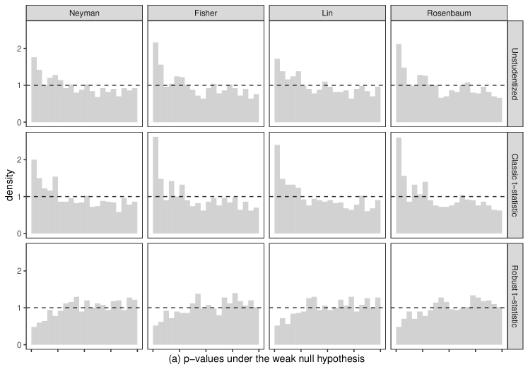
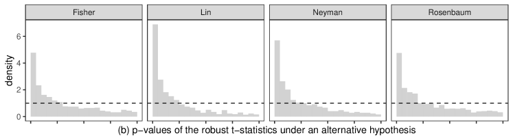
Figure 1: Empirical histograms of the $p_{\textsc{frt},\textup{str}}$’s with 20 bins in $(0,1)$.

Application

Chong et al. (2016) conducted a randomized experiment on 219 students of a rural secondary school in the Cajamarca district of Peru during the 2009 school year. They first provided the village with free iron supplements and trained the local staffs to distribute one free iron pill to any adolescent who requested one in person. They then randomly assigned the students to three arms with three different types of videos: in the first video, a popular soccer player was encouraging the use of iron supplements to maximize energy (“soccer” arm); in the second video, a physician was encouraging the use of iron supplements to improve overall health (“physician” arm); the third video did not mention iron and served as the control (“control” arm). The experiment was stratified by the class level from 1 to 5. The treatment group sizes within classes are shown in the matrix below:

$$\bordermatrix{&\text{class 1}&\text{class 2}&\text{class 3}&\text{class 4}&\text{class 5}\cr\text{soccer}&16&19&15&10&10\cr\text{physician}&17&20&15&11&10\cr\text{control}&15&19&16&12&10\cr}.$$

One outcome of interest is the average grade in the third and fourth quarters of 2009, and an important background covariate is the anemia status at baseline. We make pairwise comparisons of the “soccer” arm versus the “control” arm and the “physician” arm versus the “control” arm. We also compare frts with and without adjusting for the covariate of baseline anemia status. We use their data set to illustrate frts under complete randomization and stratified randomization. The ten subgroup analyses use frts for complete randomization within each class level. The two overall analyses use frts for stratified randomization averaging over all class levels.

Table 2: Re-analyzing the data from Chong et al. (2016). “n” denotes the unadjusted estimators and tests, and “l” denotes the covariate-adjusted estimators and tests. The “$p_{\textsc{frt}}$” values for the overall comparisons in the last two rows are all $p_{\textsc{frt},\text{str}}$.

(a) soccer versus control

	est	s.e.	$p_{\text{normal}}$	$p_{\textsc{frt}}$
class 1
n	0.051	0.502	0.919	0.924
l	0.050	0.489	0.919	0.929
class 2
n	$-0.158$	0.451	0.726	0.722
l	$-0.176$	0.452	0.698	0.700
class 3
n	0.005	0.403	0.990	0.989
l	$-0.096$	0.385	0.803	0.806
class 4
n	$-0.492$	0.447	0.271	0.288
l	$-0.511$	0.447	0.253	0.283
class 5
n	0.390	0.369	0.291	0.314
l	0.443	0.318	0.164	0.186
all
n	$-0.051$	0.204	0.802	0.800
l	$-0.074$	0.200	0.712	0.712

(b) physician versus control

	est	s.e.	$p_{\text{normal}}$	$p_{\textsc{frt}}$
class 1
n	0.567	0.426	0.183	0.192
l	0.588	0.418	0.160	0.174
class 2
n	0.193	0.438	0.659	0.666
l	0.265	0.409	0.517	0.523
class 3
n	1.305	0.494	0.008	0.012
l	1.501	0.462	0.001	0.003
class 4
n	$-0.273$	0.413	0.508	0.515
l	$-0.313$	0.417	0.454	0.462
class 5
n	$-0.050$	0.379	0.895	0.912
l	$-0.067$	0.279	0.811	0.816
all
n	0.406	0.202	0.045	0.047
l	0.463	0.190	0.015	0.017

Table 2 shows the point estimators, the robust standard errors, the $p$-values based on large-sample approximations of the robust $t$-statistics, and the $p$-values based on frts. In most strata, covariate adjustment decreases the standard errors since the baseline anemia status is predictive of the outcome. Two exceptions are the pairwise comparison of the “soccer” arm versus the “control” arm within class 2 and the pairwise comparison of the “physician” arm versus the “control” arm within class 4, with differences both in the third digit after the decimal point. This is likely due to the small group sizes within these strata, leaving the asymptotic approximations dubious. The $p$-values from the large-sample approximations and frts are close with the latter being slightly larger in most cases. Based on the theory, the $p$-values based on frts should be trusted more given their additional guarantee of finite-sample exactness under the strong null hypothesis. This becomes important in this example given the relatively small group sizes within strata.

Bind and Rubin (2020) suggested reporting not only the $p$-values but also the randomization distributions of the test statistics when conducting frt. Echoing their recommendation, we show in Figure 2 the histograms of the randomization distributions of the robust $t$-statistics alongside the asymptotic approximations. The discrepancy is quite clear in the subgroup analyses yet becomes unnoticeable after averaged over all class levels. Overall, the $p$-values based on large-sample approximations do not differ substantially from those based on frts in this application. The two approaches yield coherent conclusions: the video with a physician telling the benefits of iron supplements improved the academic performance and the effect was most significant among students in class 3; in contrast, the video with a popular soccer player telling the benefits did not have any significant effect.

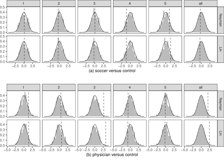
Figure 2: Randomization distributions based on $5\times 10^{4}$ Monte Carlo simulations versus $\mathcal{N}(0,1)$.

Discussion

Echoing Fisher (1935), Proschan and Dodd (2019), Young (2019), and Bind and Rubin (2020), we believe frt should be the default choice for analyzing experimental data given its flexibility to accommodate complex randomization schemes and arbitrary outcome generating processes. We established in this paper the theory for covariate adjustment in frt under complete randomization, cluster randomization, stratified randomization, and rerandomization using the Mahalanobis distance, respectively, with final recommendations of the test statistics summarized in Table 3. Equipped with the finite-sample exactness under the strong null hypothesis, the recommended frts promise an additional guarantee under the weak null hypothesis and strictly dominate the counterparts based on large-sample approximations. A key point to note is that robust studentization is necessary for the resulting frt to retain asymptotic validity when only the weak null hypothesis holds. A casual choice of the test statistic is likely to lead to misleading conclusions.

Table 3: Final recommendations for frt and test statistic $\hat{\tau}_{*}/\tilde{\textup{se}}_{*}$ in different experiments.

design	presence of covariates		other comments
	aaanoaaa	yes
complete randomization	$*=\textsc{n}$	$*=\textsc{l}$
cluster randomization	$*=\textsc{n}$	$*=\textsc{l}$	use cluster total outcomes
stratified randomization	$*=\textsc{n}$	$*=\textsc{l}$	weighted average over strata
ReM, complete design information		$*=\textsc{l}$
ReM, incomplete design information	$*=\textsc{n}$	$*=\textsc{l}$	use $p_{\textsc{frt}}$ not $p_{\textsc{frt},\mathcal{A}}$

We conjecture that the strategy of appropriately studentizing an efficient, covariate-adjusted estimator works for frt in general experiments as well (e.g., Dasgupta et al. 2015; Lu 2016; Mukerjee et al. 2018; Middleton 2018; Fogarty 2018a, b). This strategy works for estimators with normal limiting distributions and may also work for estimators with non-normal limiting distributions as shown in the asymptotic theory of rerandomization. Cohen and Fogarty (2020)’s prepivoting approach may work more broadly but we leave the general theory to future research.

We focused on procedures based on ols. It is of great interest to extend the theory to high dimensional settings (Bloniarz et al. 2016; Lei and Ding 2020), nonlinear models (Zhang et al. 2008; Moore and van der Laan 2009; Moore et al. 2011; Jiang et al. 2019; Guo and Basse 2020), and even estimators based on machine learning algorithms (Wager et al. 2016; Wu and Gagnon-Bartsch 2018; Farrell et al. 2021; Chen et al. 2020).

If the main parameter of interest is the average treatment effect, the asymptotic theory inevitably involves some moment conditions. Without these conditions, the inference becomes challenging (Bahadur and Savage 1956), and frt may not control type one error rates even asymptotically with heavy-tailed outcomes. An alternative class of frts use rank statistics to gain robustness with respect to outliers (Lehmann 1975; Rosenbaum 2002). Although different rank statistics always work under the strong null hypothesis, they in general target parameters other than the average treatment effect (e.g., Rosenbaum 1999, 2003; Chung and Romano 2016). Chung and Romano (2016) proposed to studentize the Wilcoxon statistic in a permutation test, shedding light on the general theory of frt with rank statistics.

Section S1 discusses the extensions to the super-population framework and other permutation tests based on linear models.

Section S2 reviews the notation and some algebraic facts that hold for arbitrary data generating process. We omit the proofs because they are straightforward. It contains Lemma S1 on the univariate ols fit, a basic yet powerful tool in later proofs when coupled with the Frisch–Waugh–Lovell theorems for both the regression coefficients and standard errors [Ding, 2020]. When referring to the Frisch–Waugh–Lovell theorems, we will simply say “by fwl.”

Section S3 reviews the central limit theorems under complete randomization and random permutation, and gives a new finite population strong law of large numbers that works under not only simple random sampling and complete randomization but also rejective sampling and ReM [Fuller, 2009, Morgan and Rubin, 2012].

Section S4 gives the proofs of the main results under complete randomization.

Section S5 gives the proofs of the results under ReM.

Section S6 gives the proofs of the results related to the extensions to the super-population framework and permutation tests based on linear models in Section S1.

Extensions to super-population inference

S1.1 Overview

We extend in this section the theory to the super-population framework and show the validity of the proposed procedures when the potential outcomes are independent draws from a super population. Further, the proposed procedures, though model-free in theory, make use of the ols coefficients and $t$-statistics for easy implementation. It is thus curious to study their connections with existing permutation tests for coefficients in linear models [Freedman and Lane, 1983, ter Braak, 1992, Kennedy, 1995, Manly, 1997, DiCiccio and Romano, 2017], as reviewed by Anderson and Legendre [1999], Anderson and Robinson [2001], and Lei and Bickel [2020]. We evaluate the operating characteristics of these permutation tests for testing the treatment effects, and demonstrate the superiority of frt by various criteria. Among them, the recent proposal by DiCiccio and Romano [2017] is the closest to frt and coincides in procedure with frt based on Fisher [1935]’s estimator studentized by the robust standard error. Recall from Corollary 3 in the main text that this frt does not necessarily improve the power when testing the treatment effects. A possible improvement is to include adding the treatment-covariates interactions into the linear model, such that it coincides with our final recommendation of frt based on Lin [2013]’s estimator studentized by the robust standard error. DiCiccio and Romano [2017]’s original theory was developed under the linear model assumption for testing whether a coefficient is zero. Our extension provides an additional justification for it under the potential outcomes framework for testing the treatment effects.

S1.2 Connection with the super-population framework

In addition to the finite-population perspective that conditions on the potential outcomes for inferences, it is also conventional to view the experimental units as random samples from a super population [Tsiatis et al., 2008, Berk et al., 2013, Bugni et al., 2018, Negi and Wooldridge, 2021, Ye et al., 2020a]. We now extend the discussion to this framework and examine the operating characteristics of the proposed strategies for conducting frt on random potential outcomes. Assume $\{Y_{i}(0),Y_{i}(1),Z_{i},x_{i}\}_{i=1}^{N}$ are independent and identically distributed (iid) samples from a super population. With a slight abuse of notation, let $\tau=E\{Y_{i}(1)-Y_{i}(0)\}$ be the population average treatment effect throughout Section S1.2. The goal is to test

$$H_{0}:\tau=0$$

as the analog of $H_{0{\textsc{n}}}$ in the finite-population setting.

Recall $p_{z}=N_{z}/N$ as the treatment proportions for $z=0,1$. Without introducing new notation, let $p_{z}$ also denote $P(Z_{i}=z)$, equaling the probability limit of $N_{z}/N$ as $N$ goes to infinity. Let

$$\mu_{z}=E\{Y_{i}(z)\},\quad\sigma^{2}_{z}=\operatorname{var}\{Y_{i}(z)\},\quad\mu_{x}=E(x_{i}),\quad\sigma_{x}^{2}=\operatorname{cov}(x_{i}),\quad\sigma_{xY(z)}=\operatorname{cov}\{x_{i},Y_{i}(z)\}$$

be the first two moments of the potential outcomes and covariates. We impose the following conditions under the super-population framework.

Condition S1.

$\{Y_{i}(0),Y_{i}(1),Z_{i},x_{i}\}_{i=1}^{N}$ are iid draws from the population with (i) $E(\|x_{i}\|_{4}^{4})\leq\infty$, $E\{Y^{4}_{i}(z)\}\leq\infty$, $E\{\|x_{i}Y_{i}(z)\|_{4}^{4}\}\leq\infty$, $\sigma_{z}^{2}-\sigma_{xY(z)}^{\mathrm{\scriptscriptstyle T}}(\sigma_{x}^{2})^{-1}\sigma_{xY(z)}>0$ for $z=0,1$, and (ii) $Z_{i}\ \begin{picture}(9.0,8.0)\put(0.0,0.0){\line(1,0){9.0}} \put(3.0,0.0){\line(0,1){8.0}} \put(6.0,0.0){\line(0,1){8.0}} \end{picture}\ \{Y_{i}(0),Y_{i}(1),x_{i}\}$.

With a slight abuse of notation, let $\gamma_{z}=(\sigma_{x}^{2})^{-1}\sigma_{xY(z)}$ be the coefficient of $x_{i}$ in the population ols fit of $Y_{i}(z)$ on $(1,x_{i})$, and let $a_{i}(z)=Y_{i}(z)-\mu_{z}-(x_{i}-\mu_{x})^{\mathrm{\scriptscriptstyle T}}(p_{1}\gamma_{1}+p_{0}\gamma_{0})$ and $b_{i}(z)=Y_{i}(z)-\mu_{z}-(x_{i}-\mu_{x})^{\mathrm{\scriptscriptstyle T}}\gamma_{z}$ be the residuals. Let $\sigma^{2}_{a(z)}$ and $\sigma_{b(z)}^{2}$ be the variances of $a_{i}(z)$ and $b_{i}(z)$, respectively. Negi and Wooldridge [2021] reviewed the asymptotic distributions of the estimators as $\sqrt{N}(\hat{\tau}_{*}-\tau)\rightsquigarrow\mathcal{N}(0,v_{*})\ (*={\textsc{n}},{\textsc{r}},{\textsc{f}},{\textsc{l}})$ with

$$v_{\textsc{n}}=p_{1}^{-1}\sigma^{2}_{1}+p_{0}^{-1}\sigma^{2}_{0},\quad\quad v_{\textsc{r}}=v_{\textsc{f}}=p_{1}^{-1}\sigma^{2}_{a(1)}+p_{0}^{-1}\sigma^{2}_{a(0)},\quad\quad v_{\textsc{l}}=p_{1}^{-1}\sigma_{b(1)}^{2}+p_{0}^{-1}\sigma_{b(0)}^{2}+\Delta_{\bar{x}},$$ (S1)

where $\Delta_{\bar{x}}=(\gamma_{1}-\gamma_{0})^{\mathrm{\scriptscriptstyle T}}\sigma_{x}^{2}(\gamma_{1}-\gamma_{0})$. Technically, Negi and Wooldridge [2021] did not discuss $\hat{\tau}_{\textsc{r}}$, but we can show that $\hat{\tau}_{\textsc{r}}$ has the same asymptotic distribution as $\hat{\tau}_{\textsc{f}}$. So we unify the results above. A key distinction from the finite-population analysis is that $\hat{\tau}_{\textsc{l}}$ now has extra variability due to the centering of the covariates. In contrast, other estimators do not have this extra term $\Delta_{\bar{x}}$ because they remain unchanged regardless of whether we center the covariates or not.

The extra term due to centering goes away if we condition on all covariates. But if we stick to the iid assumption in Condition S1, we must modify the standard errors for Lin [2013]’s estimator to account for $\Delta_{\bar{x}}$ [Berk et al., 2013, Negi and Wooldridge, 2021]. In particular, define $\hat{\textup{se}}_{{\textsc{l}}}^{2}$ and $\tilde{\textup{se}}_{{\textsc{l}}}^{2}$ as the classic and robust standard errors squared plus $\hat{\Delta}_{\bar{x}}/N=\hat{\theta}^{\mathrm{\scriptscriptstyle T}}S_{x}^{2}\hat{\theta}/N$, respectively, where $S_{x}^{2}$ is the sample covariance matrix of the $x_{i}$’s and $\hat{\theta}=\hat{\gamma}_{{\textsc{l}},1}-\hat{\gamma}_{{\textsc{l}},0}$ is the coefficient of $Z_{i}(x_{i}-\bar{x})$ in the ols fit of $Y_{i}$ on $\{1,Z_{i},x_{i}-\bar{x},Z_{i}(x_{i}-\bar{x})\}$. We then use them to construct the studentized statistics and obtain in total twelve test statistics as in Table 1. Of interest is whether the resulting tests preserve the correct type one error rates under the super-population framework for testing $H_{0}$.

Theorem S1 gives the asymptotic sampling and randomization distributions of the twelve test statistics in Table 1. The same reasoning that underpins Corollaries 1 and 3 ensures the four robust $t$-statistics are the only options proper for testing $H_{0}$, among which $\hat{\tau}_{\textsc{l}}/\tilde{\textup{se}}_{\textsc{l}}$ enjoys the highest power. Below, $P_{\textsc{s}}\text{-}{\text{a.s.}}$ indicates a statement that holds for almost all sequences of $\{Y_{i}(0),Y_{i}(1),Z_{i},x_{i}\}_{i=1}^{N}$.

Theorem S1.

Assume Condition S1.

1. $\sqrt{N}(\hat{\tau}_{*}-\tau)\rightsquigarrow\mathcal{N}(0,v_{*})$, and $\sqrt{N}\hat{\tau}^{\pi}_{*}\rightsquigarrow\mathcal{N}(0,v_{*0})\ P_{\textsc{s}}\text{-}{\text{a.s.}}$, with $v_{*}\ (*={\textsc{n}},{\textsc{r}},{\textsc{f}},{\textsc{l}})$ defined in (S1), $v_{{\textsc{n}}0}=p_{0}^{-1}\sigma^{2}_{1}+p_{1}^{-1}\sigma^{2}_{0}+\tau^{2}$, and $v_{{\textsc{r}}0}=v_{{\textsc{f}}0}=v_{{\textsc{l}}0}=p_{0}^{-1}\sigma_{a(1)}^{2}+p_{1}^{-1}\sigma_{a(0)}^{2}+\tau^{2}.$

2. $(\hat{\tau}_{*}-\tau)/\hat{\textup{se}}_{*}\rightsquigarrow\mathcal{N}(0,c_{*})$, and $(\hat{\tau}_{*}/\hat{\textup{se}}_{*})^{\pi}\rightsquigarrow\mathcal{N}(0,1)\ P_{\textsc{s}}\text{-}{\text{a.s.}}$, with $c^{\prime}_{*}=v_{*}/(v_{*0}-\tau^{2})$ for $*={\textsc{n}},{\textsc{r}},{\textsc{f}}$, and $c^{\prime}_{\textsc{l}}=v_{\textsc{l}}/\{p_{0}^{-1}\sigma_{b(1)}^{2}+p_{1}^{-1}\sigma_{b(0)}^{2}+\Delta_{\bar{x}}\}.$

3. $(\hat{\tau}_{*}-\tau)/\tilde{\textup{se}}_{*}\rightsquigarrow\mathcal{N}(0,1)$, and $(\hat{\tau}_{*}/\tilde{\textup{se}}_{*})^{\pi}\rightsquigarrow\mathcal{N}(0,1)\ P_{\textsc{s}}\text{-}{\text{a.s.}}$ for $*={\textsc{n}},{\textsc{r}},{\textsc{f}},{\textsc{l}}$.

The sampling distributions, except for those indexed by r, are known, but the permutation distributions, especially those with corrections for $\Delta_{\bar{x}}$, are new. Intuitively, $\sigma^{2}_{z}$ mirrors the finite-population limit of $S_{z}^{2}$ in Condition 1 and affords the probability limit of $S_{z}^{2}$ under the super-population framework. The asymptotic variances of $\hat{\tau}_{*}\ (*={\textsc{n}},{\textsc{r}},{\textsc{f}})$ in Theorem S1 thus mirror their finite-population analogs in Theorem 1–3 without the conservativeness issue. In contrast, the asymptotic variance of $\hat{\tau}_{\textsc{l}}$ features the additional term $\Delta_{\bar{x}}$. The randomization distribution of $\hat{\Delta}_{\bar{x}}$ is of higher order such that the randomization distributions $(\hat{\tau}_{\textsc{l}}/\hat{\textup{se}}_{\textsc{l}})^{\pi}$ and $(\hat{\tau}_{\textsc{l}}/\tilde{\textup{se}}_{\textsc{l}})^{\pi}$ remain at $\mathcal{N}(0,1)$ even after this correction in the standard error.

Corollary S1.

Assume Condition S1. The robustly studentized $\hat{\tau}_{*}/\tilde{\textup{se}}_{*}\ (*={\textsc{n}},{\textsc{r}},{\textsc{f}},{\textsc{l}})$ are the only test statistics in Table 1 proper for testing $H_{0}$, with the limiting values of $\tilde{\textup{se}}_{\textsc{l}}^{2}/\tilde{\textup{se}}_{*}^{2}$ less than or equal to 1 for $*={\textsc{n}},{\textsc{r}},{\textsc{f}}$ $P_{\textsc{s}}\text{-}{\text{a.s.}}$.

Aronow et al. [2014] proposed an improvement on $\tilde{\textup{se}}_{\textsc{n}}$ under the finite population framework, which can be extended to $\tilde{\textup{se}}_{*}\ (*={\textsc{r}},{\textsc{f}},{\textsc{l}})$ as well. These alternatives, however, underestimate the asymptotic variances of $\hat{\tau}_{*}\ (*={\textsc{n}},{\textsc{r}},{\textsc{f}},{\textsc{l}})$ under the super-population framework. We thus do not pursue them in our recommendation.

Much recent work has been done characterizing the asymptotic behaviors of more sophisticated assignment mechanisms [e.g., Bai et al., 2021, Bugni et al., 2019, Ye et al., 2020b, Zhang and Zheng, 2020]). We leave the general theory to future work.

S1.3 Connection with permutation tests for coefficients in linear models

We unified the twelve test statistics in Table 1 as outputs from ols fits and permuted $Z$ to compute the $p$-values via frt. The procedures are similar in form to permutation tests based on linear models. Consider a linear model

$$Y=1_{N}\alpha+Z\beta+X\gamma+\epsilon$$ (S2)

that characterizes the treatment effect by the coefficient of $Z$. Testing the treatment effect reduces to testing $\beta=0$. It is standard to use the $t$-test based on the classic or robust standard error. Permutation tests, on the other hand, afford compelling alternatives due to their accuracy in finite samples [Anderson and Legendre, 1999, Anderson and Robinson, 2001]. We review here five existing permutation tests for testing $\beta=0$ under model (S2) and show their inferiority to frt with $\hat{\tau}_{\textsc{l}}/\tilde{\textup{se}}_{\textsc{l}}$ for testing the treatment effects.

S1.3.1 A review of existing permutation tests for linear models

Without introducing new symbols, let $\hat{\tau}_{\textsc{f}}$ be the coefficient of $Z$ from the ols fit of model (S2), with $\hat{\textup{se}}_{\textsc{f}}$ and $\tilde{\textup{se}}_{\textsc{f}}$ as the classic and robust standard errors. Draper and Stoneman [1966] used the square of the multiple correlation coefficient as the test statistic, and constructed the reference distribution by permuting $Z$. A recent proposal by DiCiccio and Romano [2017] used the $\hat{\tau}_{\textsc{f}}/\tilde{\textup{se}}_{\textsc{f}}$ as the test statistic and constructed the reference distribution by permuting $Z$. It coincides with frt based on $\hat{\tau}_{\textsc{f}}/\tilde{\textup{se}}_{\textsc{f}}$ in procedure and delivers asymptotically robust randomization test for $\beta=0$ under the linear model framework. Our theory gives another justification of it for testing both $H_{0{\textsc{f}}}$ and $H_{0{\textsc{n}}}$ under the potential outcomes framework. Recall from Corollary 3 that frt with $\hat{\tau}_{\textsc{f}}/\tilde{\textup{se}}_{\textsc{f}}$ does not necessarily improve the power when testing the treatment effects. A possible improvement is thus to add treatment-covariates interactions to model (S2) such that the procedure coincides with the more powerful test based on $\hat{\tau}_{\textsc{l}}/\tilde{\textup{se}}_{\textsc{l}}$. Depending on whether we condition on the covariates or treat them as iid draws from a super population, we might need to modify the robust standard error as discussed in Section S1.2.

The rest four permutation tests, on the other hand, all used the classic $\hat{\tau}_{\textsc{f}}/\hat{\textup{se}}_{\textsc{f}}$ as the test statistic yet employed distinct permutation schemes to generate the reference distributions. We review below their respective procedures to highlight the difference, and extend them to a unified theory with test statistics being the coefficients and the classic and robust $t$-statistics, respectively. For simplicity of presentation, we only give the $p$-value formulas based on their original proposals with $\hat{\tau}_{\textsc{f}}/\hat{\textup{se}}_{\textsc{f}}$ as the test statistic. Those based on $\hat{\tau}_{\textsc{f}}/\tilde{\textup{se}}_{\textsc{f}}$ and $\hat{\tau}_{\textsc{f}}$ can be derived similarly by replacing all occurrences of the classic standard errors with their robust counterparts or constant $1$.

Freedman and Lane [1983]

Let $e$ be the residual vector from the ols fit of $Y$ on $(1_{N},X)$ as the reduced model, with the fitted vector $Y-e.$ Freedman and Lane [1983] proposed to permute $e$ and obtain the $p$-value as follows:

1. Permute $e=(e_{1},\dots,e_{N})^{\mathrm{\scriptscriptstyle T}}$ to obtain $e_{\pi}$, construct $Y^{\pi}=Y-e+e_{\pi}$ as the synthetic outcomes, and compute $(\hat{\beta}_{\textsc{fl}}^{\pi},\hat{\textup{se}}_{\textsc{fl}}^{\pi},\tilde{\textup{se}}_{\textsc{fl}}^{\pi})$ as the coefficient of $Z$ and its classic and robust standard errors from the ols fit of $Y^{\pi}$ on $(1_{N},Z,X)$.

2. Compute $p_{\textsc{fl}}=|\Pi|^{-1}\sum_{\pi\in\Pi}1(|\hat{\beta}_{\textsc{fl}}^{\pi}|/\hat{\textup{se}}_{\textsc{fl}}^{\pi}\geq|\hat{\tau}_{\textsc{f}}|/\hat{\text{se}}_{\textsc{f}}).$

The pair $(Z_{i},x_{i})$ remains intact under this procedure yet gets reshuffled under frt. This exemplifies the difference between $p_{\textsc{frt}}$ and $p_{\textsc{fl}}$. Freedman and Lane [1983] first proposed the method without the intention of making it a formal test, but rather “an alternative interpretation of a reported significance level.” It now becomes a standard permutation test for coefficients in linear models [Anderson and Legendre, 1999, Anderson and Robinson, 2001].

Kennedy [1995]

Kennedy [1995] also proposed to permute $e$ with a slight modification of Freedman and Lane [1983]. Let $\delta$ be the residual vector from the ols fit of $Z$ on $(1_{N},X)$. The procedure proceeds as follows:

1. Permute $e$ to obtain $e_{\pi}$, and compute $(\hat{\beta}_{\textsc{k}}^{\pi},\hat{\textup{se}}_{\textsc{k}}^{\pi},\tilde{\textup{se}}_{\textsc{k}}^{\pi})$ as the coefficient of $\delta$ and its classic and robust standard errors from the ols fit of $e_{\pi}$ on $(1_{N},\delta)$.

2. Compute $p_{\textsc{k}}=|\Pi|^{-1}\sum_{\pi\in\Pi}1(|\hat{\beta}_{\textsc{k}}^{\pi}|/\hat{\textup{se}}_{\textsc{k}}^{\pi}\geq|\hat{\tau}_{\textsc{f}}|/\hat{\text{se}}_{\textsc{f}}).$

Kennedy [1995] and Anderson and Robinson [2001] pointed out that $\hat{\beta}_{\textsc{k}}^{\pi}=\hat{\beta}_{\textsc{fl}}^{\pi}$ due to the Frisch–Waugh–Lovell theorem whereas $\hat{\textup{se}}_{\textsc{k}}^{\pi}\neq\hat{\textup{se}}_{\textsc{fl}}^{\pi}$ and $\tilde{\textup{se}}_{\textsc{k}}^{\pi}\neq\tilde{\textup{se}}_{\textsc{fl}}^{\pi}$.

ter Braak [1992]

ter Braak [1992] proposed to permute the residuals $\epsilon_{{\textsc{f}}}$ from the ols fit of model (S2), with $Y-\epsilon_{{\textsc{f}}}$ being the fitted vector. The procedure proceeds as follows:

1. Permute $\epsilon_{{\textsc{f}}}$ to obtain $\epsilon_{{\textsc{f}},\pi}$, construct $Y^{\pi}=Y-\epsilon_{{\textsc{f}}}+\epsilon_{{\textsc{f}},\pi}$ as the synthetic outcomes, and compute $(\hat{\beta}_{\textsc{tb}}^{\pi},\hat{\textup{se}}_{\textsc{tb}}^{\pi},\tilde{\textup{se}}_{\textsc{tb}}^{\pi})$ as the coefficient of $Z$ and its classic and robust standard errors from the ols fit of $Y^{\pi}$ on $(1_{N},Z,X)$.

2. Compute $p_{\textsc{tb}}=|\Pi|^{-1}\sum_{\pi\in\Pi}1(|\hat{\beta}_{\textsc{tb}}^{\pi}-\hat{\tau}_{\textsc{f}}|/\hat{\textup{se}}_{\textsc{tb}}^{\pi}\geq|\hat{\tau}_{\textsc{f}}|/\hat{\textup{se}}_{\textsc{f}}).$

Compare tb-1 with fl-1 to see the difference in the models used for constructing the synthetic outcomes, with Freedman and Lane [1983] using the reduced model whereas ter Braak [1992] using the full model. Consequently, tb-2 differs from fl-2 in that $\hat{\beta}_{\textsc{tb}}^{\pi}$ must be centered by $\hat{\tau}_{\textsc{f}}$ under ter Braak [1992]’s procedure.

Manly [1997]

Manly [1997] proposed to permute $Y$ as follows:

1. Permute $Y$ to obtain $Y_{\pi}$; compute $(\hat{\beta}_{\textsc{m}}^{\pi},\hat{\textup{se}}_{\textsc{m}}^{\pi},\tilde{\textup{se}}_{\textsc{m}}^{\pi})$ as the coefficient of $Z$ and its classic and standard errors from the ols fit of $Y_{\pi}$ on $(1_{N},Z,X)$.

2. Compute $p_{\textsc{m}}=|\Pi|^{-1}\sum_{\pi\in\Pi}1(|\hat{\beta}_{\textsc{m}}^{\pi}|/\hat{\textup{se}}_{\textsc{m}}^{\pi}\geq|\hat{\tau}_{\textsc{f}}|/\hat{\textup{se}}_{\textsc{f}}).$

S1.3.2 Finite-sample exactness for testing $H_{0\textsc{F}}$ and properness for testing $H_{0\textsc{N}}$

The procedures in Section S1.3.1 employed distinct permutation schemes to generate the reference distributions. DiCiccio and Romano [2017] permuted $Z$, Freedman and Lane [1983] and Kennedy [1995] permuted $e$, ter Braak [1992] permuted $\epsilon_{{\textsc{f}}}$, and Manly [1997] permuted $Y$. Table S1 summarizes them.

Table S1: Five permutation tests for testing $\beta=0$ in model (S2).

procedure	$T$	model for computing $T$	$T^{\pi}$
DiCiccio and Romano [2017]	$\hat{\tau}_{\textsc{f}}/\tilde{\textup{se}}_{\textsc{f}}$	$Y\sim 1_{N}+Z_{\pi}+X$	$\hat{\tau}_{\textsc{f}}^{\pi}/\tilde{\textup{se}}_{\textsc{f}}^{\pi}$
Freedman and Lane [1983]	$\hat{\tau}_{\textsc{f}}/\hat{\textup{se}}_{\textsc{f}}$	$Y-e+e_{\pi}\sim 1_{N}+Z+X$	$\hat{\beta}_{\textsc{fl}}^{\pi}/\hat{\textup{se}}_{\textsc{fl}}^{\pi}$
Kennedy [1995]	same as above	$e_{\pi}\sim 1_{N}+\delta$	$\hat{\beta}_{\textsc{k}}^{\pi}/\hat{\textup{se}}_{\textsc{k}}^{\pi}$
ter Braak [1992]	same as above	$Y-\epsilon_{{\textsc{f}}}+\epsilon_{{\textsc{f}},\pi}\sim 1_{N}+Z+X$	$(\hat{\beta}_{\textsc{tb}}^{\pi}-\hat{\tau}_{\textsc{f}})/\hat{\textup{se}}_{\textsc{tb}}^{\pi}$
Manly [1997]	same as above	$Y_{\pi}\sim 1_{N}+Z+X$	$\hat{\beta}_{\textsc{m}}^{\pi}/\hat{\textup{se}}_{\textsc{m}}^{\pi}$

An interesting question is how they compare with frt and each other when applied to testing the treatment effects. Whereas the operating characteristics of DiCiccio and Romano [2017] follow directly from Theorem 3 due to its identicalness to frt, those of the rest four tests are less straightforward and hinge on their respective reference distributions resulting from the distinct permutation schemes.

With a slight abuse of notation, we use the random variables under the reference distributions to represent the respective procedures for the rest of this section. The finite-sample exactness for testing $H_{0{\textsc{f}}}$, on the one hand, requires exact match of the reference distribution with the sampling distribution under $H_{0{\textsc{f}}}$. The difference in permutation schemes leaves the distributions of the unstudentized $\hat{\beta}_{\textsc{fl}}^{\pi}$, $\hat{\beta}_{\textsc{k}}^{\pi}$, $\hat{\beta}_{\textsc{tb}}^{\pi}-\hat{\tau}_{\textsc{f}}$, $\hat{\beta}_{\textsc{m}}^{\pi}$ and their studentized variants distinct from those of $\hat{\tau}_{\textsc{f}}$, $\hat{\tau}_{\textsc{f}}/\hat{\textup{se}}_{\textsc{f}}$, and $\hat{\tau}_{\textsc{f}}/{\tilde{\textup{se}}_{\textsc{f}}}$ under $H_{0{\textsc{f}}}$, such that none of them is finite-sample exact for testing $H_{0{\textsc{f}}}$. Their properness and relative power for testing $H_{0{\textsc{n}}}$, on the other hand, depend on the asymptotic behaviors of the reference distributions, which are summarized below.

Theorem S2.

Assume complete randomization and Condition 1. We have

1. $\sqrt{N}\hat{\beta}_{*}^{\pi}\rightsquigarrow\mathcal{N}(0,v_{{\textsc{f}}0})$ for $*={\textsc{fl}},{\textsc{k}};\quad\sqrt{N}(\hat{\beta}_{\textsc{tb}}^{\pi}-\hat{\tau}_{\textsc{f}})\rightsquigarrow\mathcal{N}(0,v_{{\textsc{f}}0}-\tau^{2});\quad\sqrt{N}\hat{\beta}_{\textsc{m}}^{\pi}\rightsquigarrow\mathcal{N}(0,v_{{\textsc{n}}0})$;

2. $\hat{\beta}_{*}^{\pi}/\hat{\textup{se}}_{*}^{\pi}\rightsquigarrow\mathcal{N}(0,1)$ and $\hat{\beta}_{*}^{\pi}/\tilde{\textup{se}}_{*}^{\pi}{\rightsquigarrow}\mathcal{N}(0,1)$ for $*={\textsc{fl}},{\textsc{k}},{\textsc{m}}$;
   $(\hat{\beta}_{\textsc{tb}}^{\pi}-\hat{\tau}_{\textsc{f}})/\hat{\textup{se}}_{\textsc{tb}}^{\pi}\rightsquigarrow\mathcal{N}(0,1)$ and $(\hat{\beta}_{\textsc{tb}}^{\pi}-\hat{\tau}_{\textsc{f}})/\tilde{\textup{se}}_{\textsc{tb}}^{\pi}\rightsquigarrow\mathcal{N}(0,1)$

hold $P_{Z}$-a.s., recalling $v_{{\textsc{n}}0}$ and $v_{{\textsc{f}}0}$ as the asymptotic variances of $\sqrt{N}\hat{\tau}_{\textsc{n}}^{\pi}$ and $\sqrt{N}\hat{\tau}_{\textsc{f}}^{\pi}$ defined in Theorems 1 and 3, respectively.

The asymptotic distribution of $\hat{\beta}_{\textsc{fl}}^{\pi}/\hat{\textup{se}}_{\textsc{fl}}^{\pi}$ first appeared in Freedman and Lane [1983]. Anderson and Robinson [2001] generalized it and gave a sketch of the proof for all four classic $t$-statistics in Table S1. We flesh out their proofs and furnish the new results on the unstudentized coefficients and their robustly studentized variants.

Intuitively, the asymptotic variances of $\hat{\beta}_{\textsc{fl}}^{\pi}=\hat{\beta}_{\textsc{k}}^{\pi}$, $\hat{\beta}_{\textsc{tb}}^{\pi}-\hat{\tau}_{\textsc{f}}$, and $\hat{\beta}_{\textsc{m}}^{\pi}$ are proportional to the finite-population variances of $e$, $\epsilon_{{\textsc{f}}}$, and $Y$, respectively, with increasing variability in the order of $\epsilon_{{\textsc{f}}}$, $e$, and $Y$. In particular, the ols fit of the reduced model adjusts for $X$ such that $e$ is less variable than $Y$; the ols fit of the full model (S2) further adjusts for $Z$ such that $\epsilon_{{\textsc{f}}}$ is less variable than $e$. The four unstudentized test statistics elucidate the impact of different permutation schemes on the resulting reference distributions, with $\hat{\beta}_{\textsc{fl}}^{\pi}$ and $\hat{\beta}_{\textsc{k}}^{\pi}$ sharing the same limiting distribution with $\hat{\tau}_{\textsc{f}}^{\pi}$ and $\hat{\tau}_{\textsc{r}}^{\pi}$ irrespective of the true value of $\tau$, whereas $\hat{\beta}_{\textsc{m}}^{\pi}$ sharing that with $\hat{\tau}_{\textsc{n}}^{\pi}$. The limiting distribution of $\hat{\beta}_{\textsc{tb}}^{\pi}-\hat{\tau}_{\textsc{f}}$, on the other hand, coincides with that of $\hat{\tau}_{\textsc{f}}^{\pi}$ or $\hat{\tau}_{\textsc{r}}^{\pi}$ if and only if $H_{0{\textsc{n}}}$ is true.

Despite the distinction between $\hat{\beta}_{*}^{\pi}$ for $*={\textsc{fl}},{\textsc{k}},{\textsc{tb}},{\textsc{m}}$, all eight studentized statistics are asymptotically standard normal and thus coincide with the limiting distributions of $(\hat{\tau}_{\textsc{f}}/\hat{\textup{se}}_{\textsc{f}})^{\pi}$ and $(\hat{\tau}_{\textsc{f}}/{\tilde{\textup{se}}_{\textsc{f}}})^{\pi}$ under frt. Juxtapose Theorem S2 with Theorem 3 to see the four robustly studentized variants as the only options proper for testing $H_{0{\textsc{n}}}$. We state the result in Corollary S2.

Corollary S2.

Assume Condition 1 and complete randomization. The robustly studentized $\hat{\beta}_{\textsc{fl}}^{\pi}/\tilde{\textup{se}}_{\textsc{fl}}^{\pi}$, $\hat{\beta}_{\textsc{k}}^{\pi}/\tilde{\textup{se}}_{\textsc{k}}^{\pi}$, $(\hat{\beta}_{\textsc{tb}}^{\pi}-\hat{\tau}_{\textsc{f}})/\tilde{\textup{se}}_{\textsc{tb}}^{\pi}$, and $\hat{\beta}_{\textsc{m}}^{\pi}/\tilde{\textup{se}}_{\textsc{m}}^{\pi}$ are proper for testing $H_{0{\textsc{n}}}$ whereas the unstudentized and the classically studentized alternatives are not.

Despite the positive result in Corollary S2, we do not recommend these permutation tests for testing the treatment effects for several reasons. First, they are not finite-sample exact for $H_{0{\textsc{f}}}$ in the first place, such that properness under $H_{0{\textsc{n}}}$ can be a rather weak requirement. For instance, Manly [1997]’s permutation test with the unstudentized statistic yields a reference distribution far from the true distribution of $\hat{\tau}_{\textsc{f}}$ although the robust studentization repairs it asymptotically. Second, even within the scope of testing $H_{0{\textsc{n}}}$, the test statistic $\hat{\tau}_{{\textsc{f}}}/\tilde{\textup{se}}_{\textsc{f}}$ is suboptimal compared to $\hat{\tau}_{{\textsc{l}}}/\tilde{\textup{se}}_{\textsc{l}}$ and may deliver even less power than $\hat{\tau}_{\textsc{n}}/\tilde{\textup{se}}_{\textsc{n}}$ despite the extra use of covariates. Further, Corollary S2 holds under complete randomization but may not extend to general designs even asymptotically. Overall, frt is strictly superior for testing the treatment effects.

Notation and algebraic facts

Let $1_{m}$ and $0_{m}$ be the $m\times 1$ vectors of ones and zeros, respectively, and let $I_{m}$ be the $m\times m$ identity matrix. We suppress the subscript $m$ when the dimensions are clear from the context.

For $(u_{i},v_{i})_{i=1}^{N}$, where $u_{i}$ and $v_{i}$ are $m\times 1$ and $k\times 1$ vectors, respectively, let

$$\bar{u}=N^{-1}\sum_{i=1}^{N}u_{i},\quad S_{u}^{2}=(N-1)^{-1}\sum_{i=1}^{N}(u_{i}-\bar{u})(u_{i}-\bar{u})^{\mathrm{\scriptscriptstyle T}},\quad S_{uv}=(N-1)^{-1}\sum_{i=1}^{N}(u_{i}-\bar{u})(v_{i}-\bar{v})^{\mathrm{\scriptscriptstyle T}}$$

be the finite-population mean and covariance matrices of $(u_{i})_{i=1}^{N}$ with itself and $(v_{i})_{i=1}^{N}$, respectively. The matrices $S_{u}^{2}$ and $S_{uv}$ degenerate to the finite-population variance and covariance for $m=k=1$. We suppress the “finite-population” when no confusion would arise. Let $\lambda=(N-1)/N$ be the scaling factor to accommodate the difference in normalizing by $N$ or $N-1$.

S2.1 Potential outcomes and covariates

Assume standardized covariates with mean $\bar{x}=0_{J}$ and covariance matrix $S_{x}^{2}=I_{J}$ throughout the finite-population analysis to simplify the presentation. Let $X_{j}=(x_{1j},\dots,x_{Nj})^{\mathrm{\scriptscriptstyle T}}$ be the $j$th column of $X$ with mean $N^{-1}\sum_{i=1}^{N}x_{ij}=0$ and variance $(N-1)^{-1}\sum_{i=1}^{N}x_{ij}^{2}=1$. All procedures discussed in this paper are invariant to non-degenerate transformations of the covariates and thus unaffected by the standardization.

Recall $\gamma_{z}=(S_{x}^{2})^{-1}S_{xY(z)}=(N-1)^{-1}\sum_{i=1}^{N}x_{i}Y_{i}(z)$ as the coefficient of $x_{i}$ in the ols fit of $Y_{i}(z)$ on $(1,x_{i})$. Recall $S^{2}_{z}$, $S_{a(z)}^{2}$, $S_{b(z)}^{2}$, $S_{\tau}^{2}$, and $S_{\xi}^{2}$ as the finite-population variances of $Y_{i}(z)$, $a_{i}(z)=Y_{i}(z)-\bar{Y}(z)-x_{i}^{\mathrm{\scriptscriptstyle T}}(p_{1}\gamma_{1}+p_{0}\gamma_{0})$, $b_{i}(z)=Y_{i}(z)-\bar{Y}(z)-x_{i}^{\mathrm{\scriptscriptstyle T}}\gamma_{z}$, $\tau_{i}=Y_{i}(1)-Y_{i}(0)$, and $\xi_{i}=b_{i}(1)-b_{i}(0)$, respectively. Let

$$\gamma=p_{1}\gamma_{1}+p_{0}\gamma_{0},\quad S^{2}=p_{1}S_{1}^{2}+p_{0}S_{0}^{2},\quad S_{a}^{2}=p_{1}S_{a(1)}^{2}+p_{0}S_{a(0)}^{2},\quad S_{b}^{2}=p_{1}S_{b(1)}^{2}+p_{0}S_{b(0)}^{2}.$$

We have $a_{i}(z)=Y_{i}(z)-\bar{Y}(z)-x_{i}^{\mathrm{\scriptscriptstyle T}}\gamma$,

$$S_{a(z)}^{2}=S_{z}^{2}+\|\gamma\|^{2}_{2}-2\gamma_{z}^{\mathrm{\scriptscriptstyle T}}\gamma,\quad S_{a}^{2}=S^{2}-\|\gamma\|^{2}_{2},\quad S_{b(z)}^{2}=S_{z}^{2}-\|\gamma_{z}\|^{2}_{2}, S_{\xi}^{2}=S_{\tau}^{2}-\|\gamma_{1}-\gamma_{0}\|^{2}_{2},\quad\quad$$ (S3)

with $S_{a(z)}^{2}-S_{b(z)}^{2}=\|\gamma_{z}-\gamma\|^{2}_{2}\geq 0$ for $z=0,1$.

S2.2 Observed outcomes and OLS fits

Let $\hat{Y}(z)=N_{z}^{-1}\sum_{i:Z_{i}=z}Y_{i}$ and $\hat{S}_{z}^{2}=(N_{z}-1)^{-1}\sum_{i:Z_{i}=z}\{Y_{i}-\hat{Y}(z)\}^{2}$ be the mean and variance of $\{Y_{i}:Z_{i}=z\}$, respectively. Let $\hat{\tau}_{x}=\hat{x}(1)-\hat{x}(0)$ be the difference in means of the covariates under treatment and control, where $\hat{x}(z)=N_{z}^{-1}\sum_{i:Z_{i}=z}x_{i}$. Centered covariates ensure

$$\hat{x}(1)=p_{0}\hat{\tau}_{x},\quad\hat{x}(0)=-p_{1}\hat{\tau}_{x}.$$ (S4)

Let $\hat{S}_{x(z)}^{2}=(N_{z}-1)^{-1}\sum_{i:Z_{i}=z}\{x_{i}-\hat{x}(z)\}\{x_{i}-\hat{x}(z)\}^{\mathrm{\scriptscriptstyle T}}$ and $\hat{S}_{xY(z)}=(N_{z}-1)^{-1}\sum_{i:Z_{i}=z}\{x_{i}-\hat{x}(z)\}\{Y_{i}-\hat{Y}(z)\}$ be the covariance matrices of $\{x_{i}:Z_{i}=z\}$ with itself and $\{Y_{i}:Z_{i}=z\}$.

Let $\hat{Y}=N^{-1}\sum_{i=1}^{N}Y_{i}$ and $\hat{S}^{2}=(N-1)^{-1}\sum_{i=1}^{N}(Y_{i}-\hat{Y})^{2}$ be the mean and variance of $(Y_{i})_{i=1}^{N}$, respectively. They satisfy

$$\hat{Y}=p_{1}\hat{Y}(1)+p_{0}\hat{Y}(0),\quad\hat{S}^{2}=\frac{N_{1}-1}{N-1}\hat{S}^{2}_{1}+\frac{N_{0}-1}{N-1}\hat{S}^{2}_{0}+\frac{N}{N-1}p_{0}p_{1}\hat{\tau}_{\textsc{n}}^{2}.$$ (S5)

Let $\hat{S}_{xY}=(N-1)^{-1}\sum_{i=1}^{N}x_{i}Y_{i}$ be the covariance matrix of $\{(x_{i},Y_{i})\}_{i=1}^{N}$. The ols fit of $Y$ on $(1_{N},X)$ has coefficients $(\hat{Y},\hat{\gamma}_{\textsc{r}})$ and residuals $e=(e_{1},\dots,e_{N})^{\mathrm{\scriptscriptstyle T}}$ that satisfy

$$\hat{\gamma}_{\textsc{r}}=(N-1)^{-1}\sum_{i=1}^{N}x_{i}Y_{i}=\hat{S}_{xY},\quad\quad e_{i}=Y_{i}-\hat{Y}-x_{i}^{\mathrm{\scriptscriptstyle T}}\hat{\gamma}_{\textsc{r}}\quad(i=1,\ldots,N),$$

$$\hat{e}=N^{-1}\sum_{i=1}^{N}e_{i}=0,\quad\quad\hat{S}_{e}^{2}=(N-1)^{-1}\sum_{i=1}^{N}(e_{i}-\hat{e})^{2}=(N-1)^{-1}\|e\|^{2}_{2}=\hat{S}^{2}-\|\hat{\gamma}_{\textsc{r}}\|^{2}_{2}.\quad$$ (S6)

Let $\hat{e}(z)=N_{z}^{-1}\sum_{i:Z_{i}=z}e_{i}$ and $\hat{S}_{e(z)}^{2}=(N_{z}-1)^{-1}\sum_{i:Z_{i}=z}\{e_{i}-\hat{e}(z)\}^{2}$ be the sample mean and variance of $\{e_{i}:Z_{i}=z\}$ for units in treatment group $z$.

Let $\epsilon_{*}=(\epsilon_{*,1},\dots,\epsilon_{*,N})^{\mathrm{\scriptscriptstyle T}}$ be the residuals from the ols fit that generates $\hat{\tau}_{*}$, where $*={\textsc{n}},{\textsc{r}},{\textsc{f}},{\textsc{l}}$. Let $\hat{\epsilon}_{*}(z)=N_{z}^{-1}\sum_{i:Z_{i}=z}\epsilon_{*,i}$ and $\hat{S}^{2}_{*(z)}=(N_{z}-1)^{-1}\sum_{i:Z_{i}=z}\{\epsilon_{*,i}-\hat{\epsilon}_{*}(z)\}^{2}$ be the sample mean and variance of $\{\epsilon_{*,i}:Z_{i}=z\}$ under treatment $z$. They satisfy

$$\hat{S}^{2}_{{\textsc{n}}(z)}=\hat{S}^{2}_{z},\quad\hat{S}^{2}_{{\textsc{r}}(z)}=\hat{S}_{e(z)}^{2},\quad\hat{S}^{2}_{*(z)}=\hat{S}_{z}^{2}+\hat{\gamma}_{*}^{\mathrm{\scriptscriptstyle T}}\hat{S}_{x(z)}^{2}\hat{\gamma}_{*}-2\hat{\gamma}_{*}^{\mathrm{\scriptscriptstyle T}}\hat{S}_{xY(z)}\quad\text{for $*={\textsc{r}},{\textsc{f}}$},$$

$$\hat{S}^{2}_{{\textsc{l}}(z)}=\hat{S}_{z}^{2}+\hat{\gamma}_{{\textsc{l}},z}^{\mathrm{\scriptscriptstyle T}}\hat{S}_{x(z)}^{2}\hat{\gamma}_{{\textsc{l}},z}-2\hat{\gamma}_{{\textsc{l}},z}^{\mathrm{\scriptscriptstyle T}}\hat{S}_{xY(z)},$$

$$\hat{\textup{se}}_{*}^{2}=\frac{N(N_{1}-1)}{(N-2)N_{1}N_{0}}\hat{S}_{*(1)}^{2}+\frac{N(N_{0}-1)}{(N-2)N_{1}N_{0}}\hat{S}_{*(0)}^{2}\qquad\text{for $*={\textsc{n}},{\textsc{r}}$},$$

$$\tilde{\textup{se}}_{*}^{2}=\frac{N_{1}-1}{N_{1}^{2}}\hat{S}_{*(1)}^{2}+\frac{N_{0}-1}{N_{0}^{2}}\hat{S}_{*(0)}^{2}\qquad\text{for $*={\textsc{n}},{\textsc{r}}$}.$$ (S7)

The numerical expressions of $\hat{\textup{se}}_{*}^{2}$ and $\tilde{\textup{se}}_{*}^{2}$ follow from standard least squares theory and Angrist and Pischke [2009, Chapter 8]. Analogous results for $*={\textsc{f}},{\textsc{l}}$ are given in Lemma S4 and Li and Ding [2020].

S2.3 Projection matrices

Let $H$ and $H_{1}=N^{-1}1_{N}1_{N}^{\mathrm{\scriptscriptstyle T}}$ be the projection matrices onto the column spaces of $(1_{N},X)$ and $1_{N}$. Let $\delta=(I-H)Z=(\delta_{1},\dots,\delta_{N})^{\mathrm{\scriptscriptstyle T}}$ be the residuals from the ols fit of $Z$ on $(1_{N},X)$. They satisfy

$$e=(I-H)Y,\quad He=0_{N},\quad H_{1}e=0_{N},\quad H1_{N}=1_{N},\quad HX=X,$$

$$H=H_{1}+X(X^{\mathrm{\scriptscriptstyle T}}X)^{-1}X^{\mathrm{\scriptscriptstyle T}}=N^{-1}1_{N}1_{N}^{\mathrm{\scriptscriptstyle T}}+(N-1)^{-1}XX^{\mathrm{\scriptscriptstyle T}},$$

$$\delta_{i}=Z_{i}-p_{1}-\lambda^{-1}p_{1}p_{0}x_{i}^{\mathrm{\scriptscriptstyle T}}\hat{\tau}_{x},\quad\hat{\delta}=N^{-1}\sum_{i=1}^{N}\delta_{i}=0,\quad H\delta=0_{N},\quad H_{1}\delta=0_{N},$$

$$\|\delta\|_{2}^{2}=Z^{\mathrm{\scriptscriptstyle T}}(I-H)Z=N(p_{1}p_{0}-\lambda^{-1}p_{1}^{2}p_{0}^{2}\hat{\tau}_{x}^{\mathrm{\scriptscriptstyle T}}\hat{\tau}_{x}).$$ (S8)

S2.4 A lemma on the univariate OLS

Lemma S1.

Let $u=(u_{1},\dots,u_{N})^{\mathrm{\scriptscriptstyle T}}$ and $v=(v_{1},\dots,v_{N})^{\mathrm{\scriptscriptstyle T}}$ be two $N\times 1$ vectors, and let $\hat{\tau}_{0}$ be the coefficient of $v$ from the ols fit of $u$ on $v$, with the residual vector $\eta=u-v\hat{\tau}_{0}$. Let $\hat{\textup{se}}_{0}$ and $\tilde{\textup{se}}_{0}$ be the classic and robust standard errors, respectively. We have

$$\hat{\tau}_{0}=\frac{v^{\mathrm{\scriptscriptstyle T}}u}{\|v\|^{2}_{2}},\quad\ \hat{\textup{se}}_{0}^{2}=\frac{1}{N-1}\frac{\|\eta\|^{2}_{2}}{\|v\|^{2}_{2}}=\frac{1}{N-1}\left(\frac{\|u\|^{2}_{2}}{\|v\|^{2}_{2}}-\hat{\tau}_{0}^{2}\right),\quad\ \tilde{\textup{se}}_{0}^{2}=\frac{v^{\mathrm{\scriptscriptstyle T}}\operatorname{diag}(\eta_{i}^{2})v}{(\|v\|^{2}_{2})^{2}}=\frac{\eta^{\mathrm{\scriptscriptstyle T}}\operatorname{diag}(v_{i}^{2})\eta}{(\|v\|^{2}_{2})^{2}}.$$

Probability measures and basic limiting theorems

S3.1 Probability measures

Recall $T^{\pi}=T(Z_{\pi},Y(Z),X)$, where $\pi\sim\operatorname{Unif}(\Pi)$ and $Z_{\pi}\sim\operatorname{Unif}(\mathcal{Z})$, as a random variable following the randomization distribution of $T$ conditioning on $Z$. Let $\hat{\textup{se}}_{*}^{\pi}$ and $\tilde{\textup{se}}_{*}^{\pi}$ be the classic and robust standard errors of $\hat{\tau}^{\pi}_{*}$ under $Z_{\pi}$ for $*={\textsc{n}},{\textsc{r}},{\textsc{f}},{\textsc{l}}$. By definition, $\hat{\tau}^{\pi}_{*}$, $(\hat{\tau}_{*}/\hat{\textup{se}}_{*})^{\pi}=\hat{\tau}^{\pi}_{*}/\hat{\textup{se}}_{*}^{\pi}$ and $(\hat{\tau}_{*}/\tilde{\textup{se}}_{*})^{\pi}=\hat{\tau}^{\pi}_{*}/\tilde{\textup{se}}_{*}^{\pi}$ are the outputs from the ols fits of $Y$ on $(1_{N},Z_{\pi})$ for $*={\textsc{n}}$; $e$ on $(1_{N},Z_{\pi})$ for $*={\textsc{r}}$; $Y$ on $(1_{N},Z_{\pi},X)$ for $*={\textsc{f}}$; and $Y$ on $(1_{N},Z_{\pi},X,W^{\pi})$ for $*={\textsc{l}}$, respectively, where $W^{\pi}=(W_{1}^{\pi},\dots,W_{N}^{\pi})^{\mathrm{\scriptscriptstyle T}}$ with $W_{i}^{\pi}=Z_{\pi(i)}x_{i}$. Let $(\hat{S}_{*(z)}^{2})^{\pi}$ be the analogs of $\hat{S}_{*(z)}^{2}$ based on the corresponding residuals for $*={\textsc{n}},{\textsc{r}},{\textsc{f}},{\textsc{l}}$.

Index by $Z$ and s the probability measures induced by the treatment assignment and random sampling from the population under the finite and super-population frameworks, respectively. Write $P_{Z}\text{-}{\text{a.s.}}$ if a result holds for almost all sequences of $Z$ under the finite-population framework, write $P_{\textsc{s}}\text{-}{\text{a.s.}}$ if a result holds for almost all sequences of $\{Y_{i}(1),Y_{i}(0),x_{i},Z_{i}\}_{i=1}^{N}$ under the super-population framework, and write $P_{\pi}\text{-}{\text{a.s.}}$ if a result holds for almost all sequences of $\pi\sim\operatorname{Unif}(\Pi)$ conditioning on a sequence of observed data $\mathcal{D}=(Y_{i},x_{i},Z_{i})_{i=1}^{N}$. Write $P_{(Z,\pi)}\text{-}{\text{a.s.}}$ if a result holds $P_{\pi}\text{-}{\text{a.s.}}$ for almost all sequences of $Z$ under the finite-population framework.

Let $\operatorname{var}_{\infty}$ and $\operatorname{cov}_{\infty}$ be the asymptotic variance and covariance, with the probability measure clear from the context. Write $A\overset{.}{\sim}B$ for $\sqrt{N}(A-B)=o_{P,*}(1)$ for $*=Z,\pi,\textsc{s}$.

S3.2 Central limit theorems

To analyze complete randomization and ReM, we need a central limit theorem from Li and Ding [2017, Theorem 5]: Under complete randomization and Condition 1,

$$\sqrt{N}\left(\begin{array}[]{cc}\hat{\tau}_{\textsc{n}}-\tau\\ \hat{\tau}_{x}\end{array}\right)\rightsquigarrow\mathcal{N}\left\{0_{J+1},\left(\begin{array}[]{cc}v_{\textsc{n}}&p_{1}^{-1}\gamma^{\mathrm{\scriptscriptstyle T}}_{1}+p_{0}^{-1}\gamma^{\mathrm{\scriptscriptstyle T}}_{0}\\ p_{1}^{-1}\gamma_{1}+p_{0}^{-1}\gamma_{0}&(p_{1}p_{0})^{-1}I_{J}\end{array}\right)\right\},$$

recalling $v_{\textsc{n}}=p_{1}^{-1}S_{1}^{2}+p_{0}^{-1}S_{0}^{2}-S^{2}_{\tau}$ from Theorem 1. When citing this result, we will simply say “by fpclt.”

To analyze random permutation, we need the following lemma due to Hájek [1961]. To simplify the presentation, we give a version that involves slightly stronger moment conditions than Hájek [1961, Theorem 4.1].

Lemma S2.

Let $u=(u_{1},\dots,u_{N})^{\mathrm{\scriptscriptstyle T}}$ and $v=(v_{1},\dots,v_{N})^{\mathrm{\scriptscriptstyle T}}$ be two $N\times 1$ vectors of real numbers, possibly depending on $N$. Let $\bar{u}=N^{-1}\sum_{i=1}^{N}u_{i}$, $S^{2}_{u}=(N-1)^{-1}\sum_{i=1}^{N}(u_{i}-\bar{u})^{2}$, $\bar{v}=N^{-1}\sum_{i=1}^{N}v_{i}$, and $S^{2}_{v}=(N-1)^{-1}\sum_{i=1}^{N}(v_{i}-\bar{v})^{2}$ be the means and variances, respectively. We have

1. $E(N^{-1}u^{\mathrm{\scriptscriptstyle T}}v_{\pi})=\bar{u}\bar{v},\quad\operatorname{cov}(N^{-1}u^{\mathrm{\scriptscriptstyle T}}v_{\pi})=N^{-2}(N-1)S^{2}_{u}S^{2}_{v}$;

2. $\sqrt{N}(N^{-1}u^{\mathrm{\scriptscriptstyle T}}v_{\pi}-\bar{u}\bar{v})\rightsquigarrow\mathcal{N}(0,S^{2}_{u}S^{2}_{v})$ if (i) $S^{2}_{u}$ and $S^{2}_{v}$ have finite limits, and (ii) there exists an $\epsilon>0$ such that $N^{-1}\sum_{i=1}^{N}(u_{i}-\bar{u})^{2+\epsilon}\leq c_{0}$ and $N^{-1}\sum_{i=1}^{N}(v_{i}-\bar{v})^{2+\epsilon}\leq c_{0}$ for some $c_{0}<\infty$ independent of $N$.

S3.3 A finite-population strong law of large numbers

Based on Bloniarz et al. [2016, Lemma S1], Wu and Ding [2020, Lemma A3] proved a finite-population strong law of large numbers under simple random sampling. We further improve it to allow for rejective sampling in the sense of Fuller [2009], which includes simple random sampling as a special case with $a=\infty$ below. This new finite-population strong law of large numbers in Lemma S3 is useful for analyzing both complete randomization and ReM. Condition 1 ensures the sequences of $\{Y_{i}(z)\}_{i=1}^{N}$, $(x_{ij})_{i=1}^{N}$, and $\{x_{ij}Y_{i}(z)\}_{i=1}^{N}$ satisfy the condition required by Lemma S3 for all $z=0,1$ and $j=1,\ldots,J$.

Lemma S3.

Let $(W_{i},x_{i})_{i=1}^{N}$ be a sequence of finite populations with means $\bar{W}=N^{-1}\sum_{i=1}^{N}W_{i}$ and variances $S^{2}_{W}=(N-1)^{-1}\sum_{i=1}^{N}(W_{i}-\bar{W})^{2}$ for $N=1,\ldots,\infty$. Let $\mathcal{I}\subset\{1,\ldots,N\}$ be a random sample under rejective sampling, in the sense that we start with $\mathcal{I}$ as a simple random sample yet only accept it if $\hat{\tau}_{x}=|\mathcal{I}|^{-1}\sum_{i\in\mathcal{I}}x_{i}-(N-|\mathcal{I}|)^{-1}\sum_{i\not\in\mathcal{I}}x_{i}$ satisfies $\hat{\tau}_{x}^{\mathrm{\scriptscriptstyle T}}\{\operatorname{cov}(\hat{\tau}_{x})\}^{-1}\hat{\tau}_{x}<a$. Let $\hat{W}_{\mathcal{I}}=|\mathcal{I}|^{-1}\sum_{i\in\mathcal{I}}W_{i}$ and $\hat{S}^{2}_{\mathcal{I}}=(|\mathcal{I}|-1)^{-1}\sum_{i\in\mathcal{I}}(W_{i}-\hat{W}_{\mathcal{I}})^{2}$ be the sample mean and variance, respectively, and denote by $\mathcal{A}$ the event of $\hat{\tau}_{x}^{\mathrm{\scriptscriptstyle T}}\{\operatorname{cov}(\hat{\tau}_{x})\}^{-1}\hat{\tau}_{x}<a$.

Assume as $N\to\infty$, (i) $\bar{W}$ and $S^{2}_{W}$ have finite limits, (ii) there exists a $c_{0}<\infty$ independent of $N$ such that $N^{-1}\sum_{i=1}^{N}W^{4}_{i}\leq c_{0}$, (iii) $\lim_{N\to\infty}|\mathcal{I}|/N>0$, and (iv) $\lim_{N\to\infty}P(\mathcal{A})=r>0$. We have $\hat{W}_{\mathcal{I}}-\bar{W}=o(1)$ and $\hat{S}^{2}_{\mathcal{I}}-S^{2}_{W}=o(1)$ for almost all sequences of $\mathcal{I}$.

Proof of Lemma S3.

The probability measure under rejective sampling is equivalent to the probability measure under simple random sampling conditioning on $\mathcal{A}$. We take $\mathcal{I}\subset\{1,\ldots,N\}$ as a simple random sample of size $|\mathcal{I}|$ throughout the proof and reflect the rejective sampling via conditioning on $\mathcal{A}$. We proceed by verifying that there exists an $n_{0}$ such that for all $N>n_{0}$,

$$\max\big{\{}P(\hat{W}_{\mathcal{I}}-\bar{W}\geq t\mid\mathcal{A}),\ P(\hat{W}_{\mathcal{I}}-\bar{W}\leq-t\mid\mathcal{A})\big{\}}\leq 2r^{-1}\exp\left(-\frac{|\mathcal{I}|^{2}t^{2}}{4NS_{W}^{2}}\right)\ \text{for all $t\geq 0$}.$$ (S9)

The result then follows from the Borel–Cantelli lemma via identical reasoning as in the proof of Wu and Ding [2020, Lemma A3].

Let $p_{\mathcal{A}}=P(\mathcal{A})$ for notational simplicity, and let $\mathcal{A}^{c}$ be the complement of $\mathcal{A}$. The law of total probability ensures $P(\hat{W}_{\mathcal{I}}-\bar{W}\geq t)\geq p_{\mathcal{A}}\cdot P(\hat{W}_{\mathcal{I}}-\bar{W}\geq t\mid\mathcal{A})$ and $P(\hat{W}_{\mathcal{I}}-\bar{W}\leq t)\geq p_{\mathcal{A}}\cdot P(\hat{W}_{\mathcal{I}}-\bar{W}\leq t\mid\mathcal{A})$ for all $t\geq 0$, such that

$$\max\big{\{}P(\hat{W}_{\mathcal{I}}-\bar{W}\geq t\mid\mathcal{A}),\ P(\hat{W}_{\mathcal{I}}-\bar{W}\leq-t\mid\mathcal{A})\big{\}}$$

$$\quad\quad\leq p_{\mathcal{A}}^{-1}\max\big{\{}P(\hat{W}_{\mathcal{I}}-\bar{W}\geq t),\ P(\hat{W}_{\mathcal{I}}-\bar{W}\leq-t)\big{\}}\leq p_{\mathcal{A}}^{-1}\exp\left(-\frac{|\mathcal{I}|^{2}t^{2}}{4NS_{W}^{2}}\right)\quad\text{for all $t\geq 0$}$$

by Wu and Ding [2020, Lemma A2]. The sufficient condition in (S9) then follows from $\lim_{N\to\infty}p_{\mathcal{A}}=r$ such that there exists an $n_{0}$ with $p_{\mathcal{A}}\geq 2^{-1}r$ for all $N\geq n_{0}$.

∎

Finite-population inference under complete randomization

S4.1 Core lemmas

The following lemma gives some useful facts about Fisher [1935]’s analysis of covariance, i.e., the ols fit of $Y$ on $(1_{N},Z,X)$.

Lemma S4.

For $(Y_{i},x_{i},Z_{i})_{i=1}^{N}$ from arbitrary data generating process with $\bar{x}=0_{J}$, the coefficients from the ols fit of $Y$ on $(1_{N},Z,X)$ are

$$\hat{\mu}_{\textsc{f}}=\hat{Y}-p_{1}\hat{\tau}_{\textsc{f}},\quad\hat{\tau}_{\textsc{f}}=\frac{Z^{\mathrm{\scriptscriptstyle T}}(I-H)Y}{Z^{\mathrm{\scriptscriptstyle T}}(I-H)Z}=\hat{\tau}_{\textsc{n}}-\hat{\gamma}_{\textsc{f}}^{\mathrm{\scriptscriptstyle T}}\hat{\tau}_{x},\quad\hat{\gamma}_{\textsc{f}}=(X^{\mathrm{\scriptscriptstyle T}}X)^{-1}X^{\mathrm{\scriptscriptstyle T}}Y-Np_{1}p_{0}\hat{\tau}_{\textsc{f}}(X^{\mathrm{\scriptscriptstyle T}}X)^{-1}\hat{\tau}_{x},$$

respectively, with residuals $\epsilon_{{\textsc{f}},i}=Y_{i}-\hat{Y}-(Z_{i}-p_{1})\hat{\tau}_{\textsc{f}}-x_{i}^{\mathrm{\scriptscriptstyle T}}\hat{\gamma}_{\textsc{f}}$ for $i=1,\ldots,N$ and standard errors

$$\hat{\textup{se}}^{2}_{\textsc{f}}=\frac{1}{N-2-J}\left\{\frac{Y^{\mathrm{\scriptscriptstyle T}}(I-H)Y}{Z^{\mathrm{\scriptscriptstyle T}}(I-H)Z}-\hat{\tau}_{\textsc{f}}^{2}\right\},\quad\tilde{\textup{se}}^{2}_{\textsc{f}}=\frac{\eta^{\mathrm{\scriptscriptstyle T}}\operatorname{diag}(\delta_{i}^{2})\eta}{\{Z^{\mathrm{\scriptscriptstyle T}}(I-H)Z\}^{2}},$$

where $\eta=(I-H)Y-(I-H)Z\hat{\tau}_{\textsc{f}}$ and $\delta_{i}$ are the residuals from the ols fit of $Z$ on $(1_{N},X)$.

For a sequence of $Z$ that ensures $\hat{\tau}_{x}=o(1)$, $\hat{\tau}_{*}-\tau=o(1)$ for $*={\textsc{n}},{\textsc{f}}$, $N^{-1}\sum_{i=1}^{N}\|x_{i}\|_{4}^{4}=O(1)$, and $N^{-1}\sum_{i=1}^{N}\epsilon_{{\textsc{f}},i}^{4}=O(1)$ as $N$ goes to infinity, we have

$$N\hat{\textup{se}}_{\textsc{f}}^{2}-\left(p_{0}^{-1}\hat{S}_{{\textsc{f}}(1)}^{2}+p_{1}^{-1}\hat{S}_{{\textsc{f}}(0)}^{2}\right)=o(1),\quad\quad N\tilde{\textup{se}}_{\textsc{f}}^{2}-\left(p_{1}^{-1}\hat{S}_{{\textsc{f}}(1)}^{2}+p_{0}^{-1}\hat{S}_{{\textsc{f}}(0)}^{2}\right)=o(1).$$

Proof of Lemma S4.

First, let $u=e=(I-H)Y$ and $v=\delta=(I-H)Z$ in Lemma S1 to see

$$\hat{\tau}_{0}=\frac{\delta^{\mathrm{\scriptscriptstyle T}}e}{\|\delta\|^{2}_{2}},\quad\hat{\textup{se}}_{0}^{2}=\frac{1}{N-1}\left(\frac{\|e\|^{2}_{2}}{\|\delta\|^{2}_{2}}-\hat{\tau}_{\textsc{f}}^{2}\right),\quad\tilde{\textup{se}}_{0}^{2}=\frac{\eta_{0}^{\mathrm{\scriptscriptstyle T}}\operatorname{diag}(\delta_{i}^{2})\eta_{0}}{(\|\delta\|^{2}_{2})^{2}},$$

where $\eta_{0}=e-\delta\hat{\tau}_{0}$. The numerical result for $\hat{\tau}_{\textsc{f}}$, ${\hat{\textup{se}}_{\textsc{f}}}$, and ${\tilde{\textup{se}}_{\textsc{f}}}$ follows from $\hat{\tau}_{\textsc{f}}=\hat{\tau}_{0}$, $(N-2-J)\hat{\textup{se}}_{\textsc{f}}^{2}=(N-1)\hat{\textup{se}}_{0}^{2}$, and $\tilde{\textup{se}}_{\textsc{f}}^{2}=\tilde{\textup{se}}_{0}^{2}$ by fwl.

Second, let $\chi=(1_{N},Z,X)$ be the design matrix. That $N^{-1}X^{\mathrm{\scriptscriptstyle T}}Z=p_{1}p_{0}\hat{\tau}_{x}$ by (S4) ensures

$$N^{-1}\chi^{\mathrm{\scriptscriptstyle T}}\chi=\left(\begin{array}[]{ccc}1&p_{1}&0_{J}^{\mathrm{\scriptscriptstyle T}}\\ p_{1}&p_{1}&p_{1}p_{0}\hat{\tau}_{x}^{\mathrm{\scriptscriptstyle T}}\\ 0_{J}&p_{1}p_{0}\hat{\tau}_{x}&\lambda S^{2}_{x}\end{array}\right),\quad\text{with}\quad\left(\begin{array}[]{cc}1&p_{1}\\ p_{1}&p_{1}\end{array}\right)^{-1}=p_{0}^{-1}\left(\begin{array}[]{cc}1&-1\\ -1&p_{1}^{-1}\end{array}\right),$$ (S17)

such that

$$N^{-1}\chi^{\mathrm{\scriptscriptstyle T}}\chi\left(\begin{array}[]{c}\hat{\mu}_{\textsc{f}}\\ \hat{\tau}_{\textsc{f}}\\ \hat{\gamma}_{\textsc{f}}\end{array}\right)=N^{-1}\chi^{\mathrm{\scriptscriptstyle T}}Y\quad\Longleftrightarrow\quad\left(\begin{array}[]{ccc}1&p_{1}&0_{J}^{\mathrm{\scriptscriptstyle T}}\\ p_{1}&p_{1}&p_{1}p_{0}\hat{\tau}_{x}^{\mathrm{\scriptscriptstyle T}}\\ 0_{J}&p_{1}p_{0}\hat{\tau}_{x}&\lambda S^{2}_{x}\end{array}\right)\left(\begin{array}[]{c}\hat{\mu}_{\textsc{f}}\\ \hat{\tau}_{\textsc{f}}\\ \hat{\gamma}_{\textsc{f}}\end{array}\right)=\left(\begin{array}[]{c}\hat{Y}\\ p_{1}\hat{Y}(1)\\ \lambda\hat{S}_{xY}\end{array}\right).$$

Directly comparing the rows verifies $\hat{\mu}_{\textsc{f}}=\hat{Y}-p_{1}\hat{\tau}_{\textsc{f}}$, $\hat{\tau}_{\textsc{f}}=\hat{\tau}_{\textsc{n}}-\hat{\gamma}_{\textsc{f}}^{\mathrm{\scriptscriptstyle T}}\hat{\tau}_{x}$, and $\hat{\gamma}_{\textsc{f}}=(X^{\mathrm{\scriptscriptstyle T}}X)^{-1}X^{\mathrm{\scriptscriptstyle T}}Y-\lambda^{-1}p_{1}p_{0}\hat{\tau}_{\textsc{f}}(S_{x}^{2})^{-1}\hat{\tau}_{x}$. The expression of $\epsilon_{{\textsc{f}},i}$ then follows.

Third, $N^{-1}\sum_{i=1}^{N}\epsilon_{{\textsc{f}},i}^{4}=O(1)$ ensures $\hat{S}^{2}_{{\textsc{f}}(z)}=O(1)$ for $z=0,1$. With $\hat{\textup{se}}_{\textsc{f}}^{2}$ being the $(2,2)$th element of

$$\frac{\sum_{i=1}^{N}\epsilon_{{\textsc{f}},i}^{2}}{N-J-2}(\chi^{\mathrm{\scriptscriptstyle T}}\chi)^{-1},$$

the limit of $\hat{\textup{se}}_{\textsc{f}}^{2}$ follows from

$$(N-1)^{-1}\sum_{i=1}^{N}\epsilon_{{\textsc{f}},i}^{2}=\frac{N_{1}-1}{N-1}\hat{S}^{2}_{{\textsc{f}}(1)}+\frac{N_{0}-1}{N-1}\hat{S}^{2}_{{\textsc{f}}(0)}+\frac{N}{N-1}p_{0}p_{1}\{\hat{\epsilon}_{{\textsc{f}}}(1)-\hat{\epsilon}_{{\textsc{f}}}(0)\}^{2}=p_{1}\hat{S}^{2}_{{\textsc{f}}(1)}+p_{0}\hat{S}^{2}_{{\textsc{f}}(0)}+o(1)$$

and

$$(N^{-1}\chi^{\mathrm{\scriptscriptstyle T}}\chi)^{-1}=\left(\begin{array}[]{ccc}p_{0}^{-1}&-p_{0}^{-1}&0_{J}^{\mathrm{\scriptscriptstyle T}}\\ -p_{0}^{-1}&p_{0}^{-1}p_{1}^{-1}&0_{J}^{\mathrm{\scriptscriptstyle T}}\\ 0_{J}&0_{J}&(S^{2}_{x})^{-1}\end{array}\right)+o(1).$$

Further let $\Delta=\operatorname{diag}(\epsilon_{{\textsc{f}},i}^{2})$. The robust covariance estimator is $\tilde{V}_{\textsc{f}}=(\chi^{\mathrm{\scriptscriptstyle T}}\chi)^{-1}(\chi^{\mathrm{\scriptscriptstyle T}}\Delta\chi)(\chi^{\mathrm{\scriptscriptstyle T}}\chi)^{-1}$ with $\tilde{\textup{se}}_{\textsc{f}}^{2}$ as the $(2,2)$th element. That $N^{-1}\sum_{i=1}^{N}\|x_{i}\|_{4}^{4}=O(1)$ and $N^{-1}\sum_{i=1}^{N}\epsilon_{{\textsc{f}},i}^{4}=O(1)$ ensures

$$N^{-1}\chi^{\mathrm{\scriptscriptstyle T}}\Delta\chi=N^{-1}\left(\begin{array}[]{ccc}1_{N}^{\mathrm{\scriptscriptstyle T}}\Delta 1_{N}&1_{N}^{\mathrm{\scriptscriptstyle T}}\Delta Z&1_{N}^{\mathrm{\scriptscriptstyle T}}\Delta X\\ Z^{\mathrm{\scriptscriptstyle T}}\Delta 1_{N}&Z^{\mathrm{\scriptscriptstyle T}}\Delta Z&Z^{\mathrm{\scriptscriptstyle T}}\Delta X\\ X^{\mathrm{\scriptscriptstyle T}}\Delta 1_{N}&X^{\mathrm{\scriptscriptstyle T}}\Delta Z&X^{\mathrm{\scriptscriptstyle T}}\Delta X\end{array}\right)=O(1)$$

with (i) $0<1_{N}^{\mathrm{\scriptscriptstyle T}}\Delta Z=Z^{\mathrm{\scriptscriptstyle T}}\Delta Z\leq 1_{N}^{\mathrm{\scriptscriptstyle T}}\Delta 1_{N}\leq(N\sum_{i=1}^{N}\epsilon_{{\textsc{f}},i}^{4})^{1/2}=O(N)$, (ii) $X^{\mathrm{\scriptscriptstyle T}}\Delta X=\sum_{i=1}^{N}\epsilon_{{\textsc{f}},i}^{2}x_{i}x_{i}^{\mathrm{\scriptscriptstyle T}}=O(N)$, and (iii) $1_{N}^{\mathrm{\scriptscriptstyle T}}\Delta X\leq(1_{N}^{\mathrm{\scriptscriptstyle T}}\Delta 1_{N})^{1/2}(X^{\mathrm{\scriptscriptstyle T}}\Delta X)^{1/2}$ and $Z^{\mathrm{\scriptscriptstyle T}}\Delta X\leq(Z^{\mathrm{\scriptscriptstyle T}}\Delta Z)^{1/2}(X^{\mathrm{\scriptscriptstyle T}}\Delta X)^{1/2}$. This, together with $\hat{\tau}_{x}=o(1)$ in (S17), ensures

$$N\tilde{V}_{\textsc{f}}=p_{0}^{-1}\left(\begin{array}[]{ccc}1&-1&0_{J}^{\mathrm{\scriptscriptstyle T}}\\ -1&p_{1}^{-1}&0_{J}^{\mathrm{\scriptscriptstyle T}}\\ 0_{J}&0_{J}&p_{0}S_{x}^{2}\end{array}\right)N^{-1}\left(\begin{array}[]{ccc}1_{N}^{\mathrm{\scriptscriptstyle T}}\Delta 1_{N}&1_{N}^{\mathrm{\scriptscriptstyle T}}\Delta Z&1_{N}^{\mathrm{\scriptscriptstyle T}}\Delta X\\ Z^{\mathrm{\scriptscriptstyle T}}\Delta 1_{N}&Z^{\mathrm{\scriptscriptstyle T}}\Delta Z&Z^{\mathrm{\scriptscriptstyle T}}\Delta X\\ X^{\mathrm{\scriptscriptstyle T}}\Delta 1_{N}&X^{\mathrm{\scriptscriptstyle T}}\Delta Z&X^{\mathrm{\scriptscriptstyle T}}\Delta X\end{array}\right)p_{0}^{-1}\left(\begin{array}[]{ccc}1&-1&0_{J}^{\mathrm{\scriptscriptstyle T}}\\ -1&p_{1}^{-1}&0_{J}^{\mathrm{\scriptscriptstyle T}}\\ 0_{J}&0_{J}&p_{0}S_{x}^{2}\end{array}\right)+o(1)$$

with the $(2,2)$th element as

$$N\tilde{\textup{se}}_{\textsc{f}}^{2} = p_{0}^{-2}N^{-1}(-1,p_{1}^{-1})\left(\begin{array}[]{cccc}1_{N}^{\mathrm{\scriptscriptstyle T}}\Delta 1_{N}&1_{N}^{\mathrm{\scriptscriptstyle T}}\Delta Z\\ Z^{\mathrm{\scriptscriptstyle T}}\Delta 1_{N}&Z^{\mathrm{\scriptscriptstyle T}}\Delta Z\end{array}\right)\left(\begin{array}[]{c}-1\\ p_{1}^{-1}\end{array}\right)+o(1)$$

$$= p_{0}^{-2}N^{-1}\left(1_{N}^{\mathrm{\scriptscriptstyle T}}\Delta 1_{N}-p_{1}^{-1}Z^{\mathrm{\scriptscriptstyle T}}\Delta 1_{N}-p_{1}^{-1}1_{N}^{\mathrm{\scriptscriptstyle T}}\Delta Z+p_{1}^{-2}Z^{\mathrm{\scriptscriptstyle T}}\Delta Z\right)+o(1)$$

$$= (p_{0}p_{1})^{-2}N^{-1}(Z-p_{1}1_{N})^{\mathrm{\scriptscriptstyle T}}\Delta(Z-p_{1}1_{N})+o(1)$$

$$= p_{1}^{-1}\hat{S}^{2}_{{\textsc{f}}(1)}+p_{0}^{-1}\hat{S}^{2}_{{\textsc{f}}(0)}+o(1).$$

∎

Lemma S5.

Assume Condition 1 and complete randomization. As $N\to\infty$, the following results hold $P_{Z}\text{-}{\text{a.s.}}$:

1. $\hat{Y}(z)-\bar{Y}(z)=o(1),\ \ \hat{S}^{2}_{z}-S^{2}_{z}=o(1),\ \ \hat{x}(z)=o(1),\ \ \hat{S}^{2}_{x(z)}-S_{x}^{2}=o(1),\ \ \hat{S}_{xY(z)}-S_{xY(z)}=o(1)$ for $z=0,1$.

2. The sequence of finite populations $(Y_{i},Y_{i},x_{i})_{i=1}^{N}$ satisfies Condition 1 with $N^{-1}\sum_{i=1}^{N}Y_{i}^{4}=O(1)$ and $\hat{Y}-\{p_{1}\bar{Y}(1)+p_{0}\bar{Y}(0)\}=o(1)$, $\hat{S}^{2}-S^{2}-p_{1}p_{0}\tau^{2}=o(1)$, $\hat{\gamma}_{\textsc{r}}-\gamma=o(1)$, $\hat{S}_{e}^{2}-S_{a}^{2}-p_{1}p_{0}\tau^{2}=o(1)$ giving the analogs of $\bar{Y}(z)$, $S_{z}^{2}$, $\gamma_{z}$, and both $S_{a(z)}^{2}$ and $S_{b(z)}^{2}$ for $z=0,1$, respectively.

3. $\hat{e}=0,\quad\hat{S}_{e}^{2}=S_{a}^{2}+p_{1}p_{0}\tau^{2}+o(1),\quad N^{-1}\sum_{i=1}^{N}e_{i}^{4}=O(1)$.

4. $\hat{\delta}=N^{-1}\sum_{i=1}^{N}\delta_{i}=0,\quad\hat{S}_{\delta}^{2}=(N-1)^{-1}\sum_{i=1}^{N}(\delta_{i}-\hat{\delta})^{2}=p_{1}p_{0}+o(1),\quad N^{-1}\sum_{i=1}^{N}\delta_{i}^{4}=O(1)$.

5. $\hat{\mu}_{\textsc{f}}-\hat{Y}=o(1),\quad\hat{\tau}_{\textsc{f}}-\tau=o(1),\quad\hat{\gamma}_{\textsc{f}}-\gamma=o(1),$ with
   $\hat{\epsilon}_{\textsc{f}}=N^{-1}\sum_{i=1}^{N}\epsilon_{{\textsc{f}},i}=0,\quad\hat{S}_{\textsc{f}}^{2}=(N-1)^{-1}\sum_{i=1}^{N}\epsilon_{{\textsc{f}},i}^{2}=S_{a}^{2}+o(1),\quad N^{-1}\sum_{i=1}^{N}\epsilon_{{\textsc{f}},i}^{4}=O(1).$

Lemma S5 ensures it suffices to focus on the sequences of $Z$ that satisfy (a)–(e) when verifying results on almost sure convergence under $P_{Z}$.

Proof of Lemma S5.

Recall from Condition 1 that $w_{i}(z)=(S_{x}^{2})^{-1}x_{i}Y_{i}(z)=x_{i}Y_{i}(z)$ with mean and covariance matrix $\bar{w}(z)=N^{-1}\sum_{i=1}^{N}w_{i}(z)=\lambda S_{xY(z)}$ and $S^{2}_{w(z)}=(N-1)^{-1}\sum_{i=1}^{N}\{w_{i}(z)-\bar{w}(z)\}^{2}$. Its observed analog $w_{i}=x_{i}Y_{i}$ has sample means and covariance matrices $\hat{w}(z)=N_{z}^{-1}\sum_{i:Z_{i}=z}w_{i}$ and $\hat{S}^{2}_{w(z)}=(N_{z}-1)^{-1}\sum_{i:Z_{i}=z}\{w_{i}-\hat{w}(z)\}\{w_{i}-\hat{w}(z)\}^{\mathrm{\scriptscriptstyle T}}$ for $z=0,1$. Lemma S3 ensures

$$\hat{w}(z)-S_{xY(z)}=o(1)\ P_{Z}\text{-}{\text{a.s.}},\quad\hat{S}^{2}_{w(z)}-S^{2}_{w(z)}=o(1)\ P_{Z}\text{-}{\text{a.s.}}$$ (S23)

under Condition 1. The result for $\hat{Y}(z)$, $\hat{S}_{z}^{2}$, $\hat{x}(z)$, and $\hat{S}_{x(z)}^{2}$ in statement (a) follows from Lemma S3 directly. The result for $\hat{S}_{xY(z)}$ then follows from

$$\hat{S}_{xY(z)}=(N_{z}-1)^{-1}\sum_{i:Z_{i}=z}\{x_{i}-\hat{x}(z)\}\{Y_{i}-\hat{Y}(z)\}=\frac{N_{z}}{N_{z}-1}\hat{w}(z)-\frac{N_{z}}{N_{z}-1}\hat{x}(z)\hat{Y}(z).$$

This verifies statement (a) and (S23) hold $P_{Z}\text{-}{\text{a.s.}}$, such that it suffices to verify statements (b)–(d) hold for $Z$’s that satisfy statement (a) and (S23). Fix one such sequence for the rest of proof.

For statement (b), the correspondence between the analogs follows from definitions with the analogs of $a_{i}(z)$ and $b_{i}(z)$ given by $Y_{i}-\hat{Y}-x_{i}^{\mathrm{\scriptscriptstyle T}}\hat{\gamma}_{\textsc{r}}=e_{i}$ ensured by (S2.2). The limits of $\hat{Y}$ and $\hat{S}^{2}$ follow from statement (a) and (S5). With $(w_{i},w_{i})$ as the analogs of $\{w_{i}(1),w_{i}(0)\}$ in the finite population $(Y_{i},Y_{i},x_{i})_{i=1}^{N}$, the limits of $\hat{w}=N^{-1}\sum_{i=1}^{N}w_{i}$ and $\hat{S}^{2}_{w}=(N-1)^{-1}\sum_{i=1}^{N}(w_{i}-\hat{w})(w_{i}-\hat{w})^{\mathrm{\scriptscriptstyle T}}$ follow from (S23) and applying (S5) entry-wise. This in turn ensures $\hat{S}_{xY}$, as the analog of $S_{xY(z)}$, satisfies $\hat{S}_{xY}=\hat{\gamma}_{\textsc{r}}=\lambda^{-1}\hat{w}=\gamma+o(1)$ with $\hat{S}_{e}^{2}=\hat{S}^{2}-\|\hat{\gamma}_{\textsc{r}}\|^{2}_{2}$ having finite positive limit $S^{2}+p_{1}p_{0}\tau^{2}-\|\gamma\|^{2}_{2}=S^{2}_{a}+p_{1}p_{0}\tau^{2}$ by (S3) and (S2.2). This verifies Condition 1(ii). Further, $N^{-1}\sum_{i=1}^{N}Y_{i}^{4}\leq N^{-1}\sum_{i=1}^{N}\{Y^{4}_{i}(1)+Y^{4}_{i}(0)\}\leq 2c_{0}$; likewise for $N^{-1}\sum_{i=1}^{N}\|w_{i}\|_{4}^{4}\leq 2c_{0}$. This verifies Condition 1(iii) and hence statement (b).

For statement (c), that $\hat{e}=0$ follows from (S2.2) and the variance follows from statement (b). Further, $\hat{\gamma}_{\textsc{r}}=\gamma+o(1)$ from statement (b) ensures $\|\hat{\gamma}_{\textsc{r}}\|_{\infty}=O(1)$ such that $(x_{i}^{\mathrm{\scriptscriptstyle T}}\hat{\gamma}_{\textsc{r}})^{4}\leq c_{1}\|x_{i}\|_{4}^{4}$ for some $c_{1}$ independent of $N$. This, together with $e_{i}^{4}=(e_{i}^{2})^{2}\leq\{2(Y_{i}-\hat{Y})^{2}+2(x_{i}^{\mathrm{\scriptscriptstyle T}}\hat{\gamma}_{\textsc{r}})^{2}\}^{2}\leq 8\{(Y_{i}-\hat{Y})^{4}+(x_{i}^{\mathrm{\scriptscriptstyle T}}\hat{\gamma}_{\textsc{r}})^{4}\}$, ensures $N^{-1}\sum_{i=1}^{N}e_{i}^{4}=O(1)$ and hence statement (c).

For statement (d), the limit of $\hat{S}^{2}_{\delta}$ follows from (S8) and $\hat{\tau}_{x}=0_{J}+o(1)$ by statement (a). With $\delta_{i}=Z_{i}-p_{1}-\lambda^{-1}p_{1}p_{0}x_{i}^{\mathrm{\scriptscriptstyle T}}\hat{\tau}_{x}$ from (S8), we have $\delta_{i}^{4}\leq 8\{(Z_{i}-p_{1})^{4}+(\lambda^{-1}p_{1}p_{0}x_{i}^{\mathrm{\scriptscriptstyle T}}\hat{\tau}_{x})^{4}\}$ and hence $N^{-1}\sum_{i=1}^{N}\delta_{i}^{4}=O(1)$ by the same reasoning as that for $N^{-1}\sum_{i=1}^{N}e_{i}^{4}=O(1)$ in statement (c).

Statement (e) follows from $N^{-1}Z^{\mathrm{\scriptscriptstyle T}}(I-H)Y=N^{-1}\sum_{i=1}^{N}\delta_{i}Y_{i}=p_{1}\hat{Y}(1)-p_{1}\hat{Y}-p_{1}p_{0}\hat{\gamma}_{\textsc{r}}^{\mathrm{\scriptscriptstyle T}}\hat{\tau}_{x}=p_{1}p_{0}\hat{\tau}_{\textsc{n}}-p_{1}p_{0}\hat{\gamma}_{\textsc{r}}^{\mathrm{\scriptscriptstyle T}}\hat{\tau}_{x}$ and $N^{-1}Z(I-H)Z=p_{1}p_{0}+o(1)$ by (S8). This ensures $\hat{\tau}_{\textsc{f}}=\tau+o(1)$ by Lemma S4 and thus the result on $\hat{\mu}_{\textsc{f}}$ and $\hat{\gamma}_{\textsc{f}}$. Further, replace $Y_{i}$ with $\epsilon_{{\textsc{f}},i}$ in (S5) to see

$$\hat{S}_{\textsc{f}}^{2}=\frac{N_{1}-1}{N-1}\hat{S}_{{\textsc{f}}(1)}^{2}+\frac{N_{0}-1}{N-1}\hat{S}_{{\textsc{f}}(0)}^{2}+\frac{N}{N-1}p_{0}p_{1}\left\{\hat{\epsilon}_{{\textsc{f}}}(1)-\hat{\epsilon}_{{\textsc{f}}}(0)\right\}^{2},$$

where $\hat{S}^{2}_{{\textsc{f}}(z)}=S_{a(z)}^{2}+o(1)$ by (S3) and (S2.2), and $\hat{\epsilon}_{{\textsc{f}}}(1)-\hat{\epsilon}_{{\textsc{f}}}(0)=\hat{\tau}_{\textsc{n}}-\hat{\tau}_{\textsc{f}}-\hat{\tau}_{x}^{\mathrm{\scriptscriptstyle T}}\hat{\gamma}_{\textsc{f}}=o(1)$ by $\epsilon_{{\textsc{f}},i}=Y_{i}-\hat{Y}-(Z_{i}-p_{1})\hat{\tau}_{\textsc{f}}-x_{i}^{\mathrm{\scriptscriptstyle T}}\hat{\gamma}_{\textsc{f}}$ from Lemma S4. We have $\hat{\epsilon}_{\textsc{f}}=0$ and $N^{-1}\sum_{i=1}^{N}\epsilon_{{\textsc{f}},i}^{4}\leq 27\{N^{-1}\sum_{i=1}^{N}(Y_{i}-\hat{Y})^{4}+N^{-1}\sum_{i=1}^{N}Z_{i}-p_{1})^{4}\hat{\tau}_{\textsc{f}}^{4}+N^{-1}\sum_{i=1}^{N}(x_{i}^{\mathrm{\scriptscriptstyle T}}\hat{\gamma}_{\textsc{f}})^{4}\}=O(1)$ by the Cauchy–Schwarz inequality. ∎

Technically, the first strategy by Rosenbaum [2002] takes $e$ as the fixed input for conducting frt and thus has no counterpart for $\hat{\gamma}_{\textsc{r}}$ under $Z_{\pi}$. Nevertheless, the procedure is identical to one that takes $(Y_{i},x_{i})_{i=1}^{N}$ as the fixed input, regresses $Y$ on $(1_{N},X)$ to generate $e^{\pi}=e$ and $\hat{\gamma}_{\textsc{r}}^{\pi}=\hat{\gamma}_{\textsc{r}}$ independent of $Z_{\pi}$, and then regresses $e^{\pi}=e$ on $(1_{N},Z_{\pi})$ to generate $\hat{\tau}_{\textsc{r}}^{\pi}$, $\hat{\textup{se}}_{\textsc{r}}^{\pi}$, and $\tilde{\textup{se}}_{\textsc{r}}^{\pi}$. This unifies the four procedures, $*={\textsc{n}},{\textsc{r}},{\textsc{f}},{\textsc{l}}$, as all taking $(Y_{i},x_{i})_{i=1}^{N}$ as the fixed input for conducting frt. We take this perspective to simplify the presentation.

Lemma S6.

Assume Condition 1 and complete randomization.

1. $\hat{\gamma}_{*}-\gamma=o(1)$ for $*={\textsc{r}},{\textsc{f}},\quad\hat{\gamma}_{\textsc{l}}-(p_{0}\gamma_{1}+p_{1}\gamma_{0})=o(1)$,
   $N{\hat{\textup{se}}_{\textsc{n}}}^{2}-(p_{1}p_{0})^{-1}S^{2}=o(1),\quad N\tilde{\textup{se}}_{\textsc{n}}^{2}-\left(p_{1}^{-1}S_{1}^{2}+p_{0}^{-1}S_{0}^{2}\right)=o(1),$
   $N\hat{\textup{se}}_{*}^{2}-(p_{1}p_{0})^{-1}S_{a}^{2}=o(1),\quad N\tilde{\textup{se}}_{*}^{2}-(p_{1}^{-1}S_{a(1)}^{2}+p_{0}^{-1}S_{a(0)}^{2})=o(1)\quad\text{for $*={\textsc{r}},{\textsc{f}}$}$,
   $N\hat{\textup{se}}_{\textsc{l}}^{2}-(p_{1}p_{0})^{-1}S_{b}^{2}=o(1),\quad N\tilde{\textup{se}}_{\textsc{l}}^{2}-(p_{1}^{-1}S_{b(1)}^{2}+p_{0}^{-1}S_{b(0)}^{2})=o(1)$

   hold $P_{Z}\text{-}{\text{a.s.}}$, with $N\hat{\textup{se}}_{*}^{2}$ and $N\tilde{\textup{se}}_{*}^{2}$ all having positive finite limits.

2. $\hat{\gamma}_{*}^{\pi}-\gamma=o(1)\quad\text{for $*={\textsc{r}},{\textsc{f}},{\textsc{l}}$}$, with $\hat{\gamma}_{\textsc{r}}^{\pi}=\hat{\gamma}_{\textsc{r}}$,
   $N({\hat{\textup{se}}_{\textsc{n}}}^{2})^{\pi}-(p_{1}p_{0})^{-1}S^{2}-\tau^{2}=o(1),\quad N(\tilde{\textup{se}}_{\textsc{n}}^{2})^{\pi}-(p_{1}p_{0})^{-1}S^{2}-\tau^{2}=o(1)$,
   $N(\hat{\textup{se}}^{2}_{*})^{\pi}-(p_{1}p_{0})^{-1}S_{a}^{2}-\tau^{2}=o(1),\quad N(\tilde{\textup{se}}^{2}_{*})^{\pi}-(p_{1}p_{0})^{-1}S_{a}^{2}-\tau^{2}=o(1)\quad\text{ for $*={\textsc{r}},{\textsc{f}},{\textsc{l}}$}$

   hold $P_{(Z,\pi)}\text{-}{\text{a.s.}}$, with $N(\hat{\textup{se}}_{*}^{2})^{\pi}$ and $N(\tilde{\textup{se}}_{*}^{2})^{\pi}$ all having positive finite limits.

Lin [2013, Theorem 2] showed $N\hat{\textup{se}}_{\textsc{f}}^{2}-(p_{0}^{-1}S_{a(1)}^{2}+p_{1}^{-1}S_{a(0)}^{2})=o_{P,Z}(1)$ and $N\tilde{\textup{se}}_{\textsc{f}}^{2}-(p_{1}^{-1}S_{a(1)}^{2}+p_{0}^{-1}S_{a(0)}^{2})=o_{P,Z}(1)$ as the probability limits. Lemma S6 strengthens the results to almost sure convergence.

Proof of Lemma S6.

Lemma S5 ensures that it suffices to verify the result for sequences of $Z$ that satisfy Lemma S5 statements (a)–(e). Fix one such sequence for the rest of the proof.

For statement (a) regarding the sampling distributions, the limits of $\hat{\gamma}_{*}$ follow from $\hat{\gamma}_{\textsc{r}}=(S^{2}_{x})^{-1}\hat{S}_{xY}$, $\hat{\gamma}_{\textsc{f}}=\hat{\gamma}_{\textsc{r}}-\lambda^{-1}p_{1}p_{0}\hat{\tau}_{\textsc{f}}(S_{x}^{2})^{-1}\hat{\tau}_{x}$, and $\hat{\gamma}_{\textsc{l}}=p_{0}\hat{\gamma}_{{\textsc{l}},1}+p_{1}\hat{\gamma}_{{\textsc{l}},0}$ with $\hat{\gamma}_{{\textsc{l}},z}=(\hat{S}_{x(z)}^{2})^{-1}\hat{S}_{xY(z)}$ by Proposition 1, where $\hat{\gamma}_{\textsc{r}}=o(1)$, $\hat{\tau}_{\textsc{f}}-\tau=o(1)$, and $\hat{\gamma}_{{\textsc{l}},z}-\gamma_{z}=o(1)$ by Lemma S5. This ensures $\hat{S}_{{\textsc{n}}(z)}^{2}-S_{z}^{2}=o(1)$, $\hat{S}_{*(z)}^{2}-S_{a(z)}^{2}=o(1)$ for $*={\textsc{r}},{\textsc{f}}$, and $\hat{S}_{{\textsc{l}}(z)}^{2}-S_{b(z)}^{2}=o(1)$ by (S3) and (S2.2), and allows us to unify the standard errors as

$$N\hat{\textup{se}}_{*}^{2}-\left(p_{0}^{-1}\hat{S}_{*(1)}^{2}+p_{1}^{-1}\hat{S}_{*(0)}^{2}\right)=o(1),\quad N\tilde{\textup{se}}_{*}^{2}-\left(p_{1}^{-1}\hat{S}_{*(1)}^{2}+p_{0}^{-1}\hat{S}_{*(0)}^{2}\right)=o(1)\ \ (*={\textsc{n}},{\textsc{r}},{\textsc{f}},{\textsc{l}}).$$

In particular, the result for $\hat{\textup{se}}_{*}^{2}$ follows from (S2.2) provided $\hat{S}_{*(z)}^{2}$ all have finite limits. The result for $\tilde{\textup{se}}_{\textsc{n}}^{2}$ and $\tilde{\textup{se}}_{\textsc{r}}^{2}$ follows from (S2.2). The result for $\tilde{\textup{se}}_{\textsc{f}}^{2}$ follows from Lemma S4 with the regularity condition ensured by Lemma S5(e). The result for $\tilde{\textup{se}}_{\textsc{l}}^{2}$ follows from Li and Ding [2020, Theorem 8] given Condition 1 implies Li and Ding [2020, Condition 1] by Wu and Ding [2020, Proposition 1]. Alternatively, almost identical algebra as in the proof of Lemma S4 for the limiting value of $N\tilde{\textup{se}}_{\textsc{f}}^{2}$ attains the same end. Condition 1(ii) and (S3) ensure the limits are all positive.

For statement (b) regarding the randomization distributions, frt takes $(Y_{i},x_{i})_{i=1}^{N}$ as the fixed input for permuting the treatment vector, and thereby induces a sequence of finite populations $(Y_{i},Y_{i},x_{i})_{i=1}^{N}$ with $Y_{i}$ as the “pseudo potential outcomes” under both treatment and control. The way we chose the fixed $Z$ further ensures $(Y_{i},Y_{i},x_{i})_{i=1}^{N}$ satisfies Condition 1. The result in statement (a) regarding the sampling distributions thus also holds for $\hat{\gamma}_{*}^{\pi}$ and $(\hat{S}^{2}_{*(z)})^{\pi}$ $P_{\pi}\text{-}{\text{a.s.}}$ if we replace $\gamma$ with $\hat{\gamma}_{\textsc{r}}$, $S_{z}^{2}$ with $\hat{S}^{2}$, and both $S_{a(z)}^{2}$ and $S_{b(z)}^{2}$ with $\hat{S}_{e}^{2}$ by the correspondence result from Lemma S5(b). The result follows from $\hat{\gamma}_{\textsc{r}}-\gamma=o(1)$, $\hat{S}^{2}-S^{2}-p_{1}p_{0}\tau^{2}=o(1)$, and $\hat{S}^{2}_{e}-S_{a}^{2}-p_{1}p_{0}\tau^{2}=o(1)$.

∎

Lemma S7.

Assume Condition 1 and complete randomization.

1. $\hat{\tau}_{\textsc{l}}\overset{.}{\sim}\hat{\tau}_{\textsc{n}}-(p_{0}\gamma_{1}+p_{1}\gamma_{0})^{\mathrm{\scriptscriptstyle T}}\hat{\tau}_{x},\quad\hat{\tau}_{\textsc{f}}\overset{.}{\sim}\hat{\tau}_{\textsc{r}}\overset{.}{\sim}\hat{\tau}_{\textsc{n}}-\gamma^{\mathrm{\scriptscriptstyle T}}\hat{\tau}_{x}$.

2. $\hat{\tau}_{\textsc{r}}^{\pi}\overset{.}{\sim}\hat{\tau}_{\textsc{f}}^{\pi}\overset{.}{\sim}\hat{\tau}_{\textsc{l}}^{\pi}\overset{.}{\sim}\hat{\tau}_{\textsc{n}}^{\pi}-\gamma^{\mathrm{\scriptscriptstyle T}}\hat{\tau}_{x}^{\pi}$ holds $P_{Z}\text{-}{\text{a.s.}}$.

Proof of Lemma S7.

First, let $\gamma_{\textsc{r}}=\gamma_{\textsc{f}}=\gamma$ and $\gamma_{\textsc{l}}=p_{0}\gamma_{1}+p_{1}\gamma_{0}$ to write $\hat{\gamma}_{*}-\gamma_{*}=o(1)\ P_{Z}\text{-}{\text{a.s.}}$ by Lemma S6. This, together with $\hat{\tau}_{*}=\hat{\tau}_{\textsc{n}}-\hat{\gamma}_{*}^{\mathrm{\scriptscriptstyle T}}\hat{\tau}_{x}$ by Proposition 1 and $\sqrt{N}\hat{\tau}_{x}\rightsquigarrow\mathcal{N}\{0_{J},(p_{0}p_{1})^{-1}I_{J}\}$ by fpclt, ensures $\sqrt{N}\left\{\hat{\tau}_{*}-(\hat{\tau}_{\textsc{n}}-\gamma_{*}^{\mathrm{\scriptscriptstyle T}}\hat{\tau}_{x})\right\}=(\hat{\gamma}_{*}-\gamma_{*})^{\mathrm{\scriptscriptstyle T}}\sqrt{N}\hat{\tau}_{x}=o_{P,Z}(1)$ by Slutsky’s theorem and hence $\hat{\tau}_{*}\overset{.}{\sim}\hat{\tau}_{\textsc{n}}-\gamma_{*}^{\mathrm{\scriptscriptstyle T}}\hat{\tau}_{x}$.

Second, Proposition 1 is algebraic and holds under the probability measure induced by $\pi$ as well. This ensures $\hat{\tau}^{\pi}_{*}=\hat{\tau}_{\textsc{n}}^{\pi}-\gamma^{\mathrm{\scriptscriptstyle T}}\hat{\tau}_{x}^{\pi}-(\hat{\gamma}_{*}^{\pi}-\gamma)^{\mathrm{\scriptscriptstyle T}}\hat{\tau}_{x}^{\pi}$ for $*={\textsc{r}},{\textsc{f}},{\textsc{l}}$, with $\hat{\gamma}_{\textsc{r}}^{\pi}=\hat{\gamma}_{\textsc{r}}=\gamma+o(1)\ P_{Z}\text{-}{\text{a.s.}}$ and $\hat{\gamma}_{*}^{\pi}-\gamma=o(1)\ P_{\pi}\text{-}{\text{a.s.}}$ for $*={\textsc{f}},{\textsc{l}}$ $P_{Z}\text{-}{\text{a.s.}}$ by Lemma S6. Almost identical reasoning as that for $\hat{\tau}_{*}$ ensures $(\hat{\gamma}_{*}^{\pi}-\gamma)^{\mathrm{\scriptscriptstyle T}}\sqrt{N}\hat{\tau}_{x}^{\pi}=o_{P,\pi}(1)$ holds $P_{Z}\text{-}{\text{a.s.}}$ for $*={\textsc{r}},{\textsc{f}},{\textsc{l}}$ and hence the result. ∎

S4.2 Proofs of the main results under the finite-population framework

Theorem 1 is a special case of Wu and Ding [2020]. We give below a unified proof.

Proof of Theorems 1–4.

First, Condition 1 ensures $S_{a(z)}^{2}$, $S_{a}^{2}$, $S_{b(z)}^{2}$, and $S_{b}^{2}$ have positive finite limits, and $S_{\xi}^{2}$ and $S_{\tau}^{2}$ have finite limits by (S3).

The result for $\hat{\tau}_{\textsc{n}}$ and $\hat{\tau}_{\textsc{n}}^{\pi}$ follows from Ding and Dasgupta [2018], with $v_{\textsc{n}}=p_{1}^{-1}S_{1}^{2}+p_{0}^{-1}S_{0}^{2}-S_{\tau}^{2}$ and $v_{{\textsc{n}}0}=\lim_{N\to\infty}(p_{1}p_{0})^{-1}\hat{S}^{2}=p_{0}^{-1}S_{1}^{2}+p_{1}^{-1}S_{0}^{2}+\tau^{2}$. This ensures $\sqrt{N}(\hat{\tau}_{\textsc{n}}-\tau)/v_{\textsc{n}}^{1/2}\rightsquigarrow\mathcal{N}(0,1)$, and $\sqrt{N}\hat{\tau}_{\textsc{n}}^{\pi}/v_{{\textsc{n}}0}^{1/2}\rightsquigarrow\mathcal{N}(0,1)$ $P_{Z}$-a.s.. The result for the studentized variants follows from

$$\begin{array}[]{ll}({\hat{\tau}_{\textsc{n}}}-\tau)/{{\hat{\textup{se}}_{\textsc{n}}}}=\sqrt{N}({\hat{\tau}_{\textsc{n}}}-\tau)/v_{\textsc{n}}^{1/2}\cdot({v_{\textsc{n}}}/{N{\hat{\textup{se}}_{\textsc{n}}}^{2}})^{1/2},&\ \hat{\tau}_{\textsc{n}}^{\pi}/{\hat{\textup{se}}_{\textsc{n}}^{\pi}}=\sqrt{N}\hat{\tau}_{\textsc{n}}^{\pi}/v_{{\textsc{n}}0}^{1/2}\cdot\{{v_{{\textsc{n}}0}}/N(\hat{\textup{se}}^{2}_{{\textsc{n}}})^{\pi}\}^{1/2},\\ ({\hat{\tau}_{\textsc{n}}}-\tau)/{\tilde{\textup{se}}_{\textsc{n}}}=\sqrt{N}({\hat{\tau}_{\textsc{n}}}-\tau)/v_{\textsc{n}}^{1/2}\cdot({v_{\textsc{n}}}/{N\tilde{\textup{se}}_{\textsc{n}}^{2}})^{1/2},&\ \hat{\tau}_{\textsc{n}}^{\pi}/{\tilde{\textup{se}}_{\textsc{n}}^{\pi}}=\sqrt{N}\hat{\tau}_{\textsc{n}}^{\pi}/v_{{\textsc{n}}0}^{1/2}\cdot\{{v_{{\textsc{n}}0}}/N(\tilde{\textup{se}}^{2}_{{\textsc{n}}})^{\pi}\}^{1/2}\end{array}$$ (S26)

by Slutsky’s theorem with $(v_{\textsc{n}}/N{\hat{\textup{se}}_{\textsc{n}}}^{2})=c^{\prime}_{\textsc{n}}+o(1)\ P_{Z}\text{-}{\text{a.s.}},\ (v_{\textsc{n}}/N\tilde{\textup{se}}_{\textsc{n}}^{2})=c_{\textsc{n}}+o(1)\ P_{Z}\text{-}{\text{a.s.}},\ v_{{\textsc{n}}0}/N(\hat{\textup{se}}^{2}_{{\textsc{n}}})^{\pi}=1+o(1)\ P_{(Z,\pi)}\text{-}{\text{a.s.}}$, and $v_{{\textsc{n}}0}/N(\tilde{\textup{se}}^{2}_{{\textsc{n}}})^{\pi}=1+o(1)\ P_{(Z,\pi)}\text{-}{\text{a.s.}}$ by Lemma S6.

For the nine covariate-adjusted variants with $*={\textsc{r}},{\textsc{f}},{\textsc{l}}$, the result for $\hat{\tau}_{*}$ and $\hat{\tau}^{\pi}_{*}$ follows from the result for $\hat{\tau}_{\textsc{n}}$ and $\hat{\tau}_{\textsc{n}}^{\pi}$, fpclt, and Lemma S7, with

$$v_{\textsc{f}}=v_{\textsc{r}} = \operatorname{var}_{\infty}(\hat{\tau}_{\textsc{r}})=v_{\textsc{n}}+(p_{1}p_{0})^{-1}\|\gamma\|^{2}_{2}-2(p_{1}^{-1}\gamma_{1}+p_{0}^{-1}\gamma_{0})^{\mathrm{\scriptscriptstyle T}}\gamma=p_{1}^{-1}S_{a(1)}^{2}+p_{0}^{-1}S_{a(0)}^{2}-S_{\tau}^{2},$$

$$v_{\textsc{l}} = \operatorname{var}_{\infty}(\hat{\tau}_{\textsc{l}})=v_{\textsc{n}}-(p_{1}p_{0})^{-1}\|p_{0}\gamma_{1}+p_{1}\gamma_{0}\|^{2}_{2}=p_{1}^{-1}S_{b(1)}^{2}+p_{0}^{-1}S_{b(0)}^{2}-S_{\xi}^{2},$$

$$v_{*0} = \operatorname{var}_{\infty}(\hat{\tau}^{\pi}_{*})=v_{{\textsc{n}}0}-(p_{1}p_{0})^{-1}\|\gamma\|^{2}_{2}=(p_{1}p_{0})^{-1}S_{a}^{2}+\tau^{2}\quad\text{for $*={\textsc{r}},{\textsc{f}},{\textsc{l}}$}$$

by (S3). This ensures $\sqrt{N}(\hat{\tau}_{*}-\tau)/{v_{*}^{1/2}}\rightsquigarrow\mathcal{N}(0,1)$, and $\sqrt{N}\hat{\tau}^{\pi}_{*}/{v_{*0}^{1/2}}\rightsquigarrow\mathcal{N}(0,1)\ P_{Z}\text{-}{\text{a.s.}}$ for $*={\textsc{r}},{\textsc{f}},{\textsc{l}}$. The result for the studentized variants then follows from Slutsky’s theorem and Lemma S6 via the same reasoning as in (S26). ∎

Proof of Proposition 1.

That $\hat{\tau}_{\textsc{r}}=\hat{\tau}_{\textsc{n}}-\hat{\tau}_{x}^{\mathrm{\scriptscriptstyle T}}\hat{\gamma}_{\textsc{r}}$ follows from (S2.2). That $\hat{\tau}_{\textsc{f}}=\hat{\tau}_{\textsc{n}}-\hat{\tau}_{x}^{\mathrm{\scriptscriptstyle T}}\hat{\gamma}_{\textsc{f}}$ and the expression for $\hat{\gamma}_{\textsc{f}}$ follows from Lemma S4. That $\hat{\tau}_{\textsc{l}}=\hat{\tau}_{\textsc{n}}-\{\hat{x}(1)\}^{\mathrm{\scriptscriptstyle T}}\hat{\gamma}_{{\textsc{l}},1}+\{\hat{x}(0)\}^{\mathrm{\scriptscriptstyle T}}\hat{\gamma}_{{\textsc{l}},0}$ for centered covariates follows from Lin [2013], which further simplifies to $\hat{\tau}_{\textsc{l}}=\hat{\tau}_{\textsc{n}}-\hat{\tau}_{x}^{\mathrm{\scriptscriptstyle T}}\hat{\gamma}_{{\textsc{l}}}$ because of (S4). ∎

Proof of Corollary 3.

The result follows from Lemma S6 with $S^{2}_{b(z)}\leq S^{2}_{a(z)}$ and $S^{2}_{b(z)}\leq S^{2}_{z}$ by (S3). ∎

FRT under ReM

Lemma S8.

Assume Condition 1. Lemmas S5–S6 also hold under ReM.

Proof.

Lemmas S5–S6 follow from the strong law of large numbers in Lemma S3 via the same reasoning as that under complete randomization, with the convergence in probability of the sample variances to their respective finite-population variances ensured by Li et al. [2018, Lemma A16]. ∎

Proof of Theorem 5.

The probability measure under ReM is equivalent to the probability measure under complete randomization conditioning on $\mathcal{A}$. We take the distribution under complete randomization as the default distribution throughout this proof, and use “$|\text{ }\mathcal{A}$” to denote the condition of either $\hat{\tau}_{x}^{\mathrm{\scriptscriptstyle T}}\{\operatorname{cov}(\hat{\tau}_{x})\}^{-1}\hat{\tau}_{x}<a$ under the sampling distribution or $(\hat{\tau}_{x}^{\pi})^{\mathrm{\scriptscriptstyle T}}\{\operatorname{cov}(\hat{\tau}_{x}^{\pi})\}^{-1}\hat{\tau}_{x}^{\pi}<a$ under the randomization distribution. As such, $T\mid\mathcal{A}$ gives the sampling distribution of $T$ under ReM, and $T^{\pi}\mid\mathcal{A}\sim T^{\pi|\mathcal{A}}$ gives the randomization distribution of $T$ under frt with ReM.

The result for $\hat{\tau}_{\textsc{l}}$, $\hat{\tau}_{\textsc{l}}/\hat{\textup{se}}_{\textsc{l}}$, and $\hat{\tau}_{\textsc{l}}/\tilde{\textup{se}}_{\textsc{l}}$ follows from the asymptotic independence between $\hat{\tau}_{\textsc{l}}$ and $\hat{\tau}_{x}$ and between $\hat{\tau}_{\textsc{l}}^{\pi}$ and $\hat{\tau}_{x}^{\pi}$ under complete randomization [Li and Ding, 2020], such that ReM in either case does not affect the limiting distributions. We verify below the result for $*={\textsc{n}},{\textsc{r}},{\textsc{f}}$ together, starting from the unstudentized $\hat{\tau}_{*}$ and $\hat{\tau}^{\pi}_{*}$ for $*={\textsc{n}},{\textsc{r}},{\textsc{f}}$ and then moving onto the studentized variants.

For the distributions of the unstudentized $\hat{\tau}_{*}$ and $\hat{\tau}^{\pi}_{*}$, where $*={\textsc{n}},{\textsc{r}},{\textsc{f}}$, Lemma S7 ensures $\hat{\tau}_{\textsc{f}}^{\pi}\overset{.}{\sim}\ \hat{\tau}_{\textsc{r}}^{\pi}\overset{.}{\sim}\hat{\tau}_{\textsc{l}}^{\pi}$ such that it suffices to verify the result for $\hat{\tau}_{\textsc{n}}$, $\hat{\tau}_{\textsc{r}}$, $\hat{\tau}_{\textsc{f}}$, and $\hat{\tau}_{\textsc{n}}^{\pi}$. Let $D\sim\mathcal{N}(0_{J},I_{J})$ and $\epsilon\sim\mathcal{N}(0,1)$ be two independent standard normals to represent

$$\sqrt{N}\hat{\tau}_{x}\rightsquigarrow v_{x}D,\quad\sqrt{N}\hat{\tau}_{x}^{\pi}\rightsquigarrow v_{x}D,\quad\sqrt{N}(\hat{\tau}_{\textsc{l}}-\tau)\rightsquigarrow v_{\textsc{l}}^{1/2}\epsilon,\quad\sqrt{N}\hat{\tau}_{\textsc{l}}^{\pi}\rightsquigarrow v_{{\textsc{l}}0}^{1/2}\epsilon,$$

where $v_{x}=(p_{1}p_{0})^{-1/2}$ by fpclt. With

$$\hat{\tau}_{\textsc{n}}\overset{.}{\sim}\hat{\tau}_{\textsc{l}}+(p_{0}\gamma_{1}+p_{1}\gamma_{0})^{\mathrm{\scriptscriptstyle T}}\hat{\tau}_{x},\quad\hat{\tau}_{\textsc{f}}\overset{.}{\sim}\hat{\tau}_{\textsc{r}}\overset{.}{\sim}\hat{\tau}_{\textsc{l}}-(p_{1}-p_{0})(\gamma_{1}-\gamma_{0})^{\mathrm{\scriptscriptstyle T}}\hat{\tau}_{x},\quad\hat{\tau}_{\textsc{n}}^{\pi}\overset{.}{\sim}\hat{\tau}_{\textsc{l}}^{\pi}+\gamma^{\mathrm{\scriptscriptstyle T}}\hat{\tau}_{x}\ P_{Z}\text{-}{\text{a.s.}}$$

also from Lemma S7, we have

$$\sqrt{N}(\hat{\tau}_{\textsc{n}}-\tau)\mid\mathcal{A} \rightsquigarrow v_{\textsc{l}}^{1/2}\epsilon+v_{x}(p_{0}\gamma_{1}+p_{1}\gamma_{0})^{\mathrm{\scriptscriptstyle T}}D\mid(\|D\|^{2}_{2}<a),$$ (S27)

$$\sqrt{N}\hat{\tau}_{\textsc{n}}^{\pi}\mid\mathcal{A} \rightsquigarrow v_{{\textsc{l}}0}^{1/2}\epsilon+v_{x}\gamma^{\mathrm{\scriptscriptstyle T}}D\mid(\|D\|^{2}_{2}<a)\quad\quad P_{Z}\text{-}{\text{a.s.}},$$ (S28)

$$\sqrt{N}(\hat{\tau}_{*}-\tau)\mid\mathcal{A} \rightsquigarrow v_{\textsc{l}}^{1/2}\epsilon-v_{x}(p_{1}-p_{0})(\gamma_{1}-\gamma_{0})^{\mathrm{\scriptscriptstyle T}}D\mid(\|D\|^{2}_{2}<a)\quad\text{for $*={\textsc{r}},{\textsc{f}}$},$$ (S29)

with

$$v_{x}(p_{0}\gamma_{1}+p_{1}\gamma_{0})^{\mathrm{\scriptscriptstyle T}}D \sim \mathcal{N}(0,v_{\textsc{n}}-v_{\textsc{l}}),\quad v_{x}\gamma^{\mathrm{\scriptscriptstyle T}}D\sim\mathcal{N}(0,v_{{\textsc{n}}0}-v_{{\textsc{l}}0}),$$

$$-v_{x}(p_{1}-p_{0})(\gamma_{1}-\gamma_{0})^{\mathrm{\scriptscriptstyle T}}D \sim \mathcal{N}(0,v_{\textsc{r}}-v_{\textsc{l}}).$$ (S30)

Let $u=(v_{\textsc{n}}-v_{\textsc{l}})^{-1/2}v_{x}(p_{0}\gamma_{1}+p_{1}\gamma_{0})$ be a unit vector with $\|u\|^{2}_{2}=1$ and $D_{\textsc{n}}=u^{\mathrm{\scriptscriptstyle T}}D\sim\mathcal{N}(0,1)$ by the first “$\sim$” in (S5). Complete $u$ into an orthogonal matrix $\Gamma_{\textsc{n}}$ with $u^{\mathrm{\scriptscriptstyle T}}$ as the first row and $D_{\textsc{n}}$ as the first element of $\Gamma_{\textsc{n}}D$. With $\Gamma_{\textsc{n}}D\sim\mathcal{N}(0_{J},I_{J})$ and $\|\Gamma_{\textsc{n}}D\|^{2}_{2}=\|D\|^{2}_{2}$, it follows from (S5) that

$$v_{x}(p_{0}\gamma_{1}+p_{1}\gamma_{0})^{\mathrm{\scriptscriptstyle T}}D\mid(\|D\|^{2}_{2}<a)\sim(v_{\textsc{n}}-v_{\textsc{l}})^{1/2}D_{\textsc{n}}\mid(\|\Gamma_{\textsc{n}}D\|^{2}_{2}<a)\sim(v_{\textsc{n}}-v_{\textsc{l}})^{1/2}\mathcal{L}.$$

Plugging this back in (S27) proves

$$\sqrt{N}(\hat{\tau}_{\textsc{n}}-\tau)\mid\mathcal{A}\rightsquigarrow v_{\textsc{l}}^{1/2}\epsilon+(v_{\textsc{n}}-v_{\textsc{l}})^{1/2}\mathcal{L}=v^{1/2}_{\textsc{n}}\big{\{}(1-\rho^{2}_{\textsc{n}})^{1/2}\cdot\epsilon+\rho_{\textsc{n}}\cdot\mathcal{L}\big{\}}=v^{1/2}_{\textsc{n}}\cdot\mathcal{U}(\rho_{\textsc{n}}).$$

The same reasoning verifies $\sqrt{N}\hat{\tau}_{\textsc{n}}^{\pi}\mid\mathcal{A}\rightsquigarrow v_{{\textsc{n}}0}^{1/2}\cdot\mathcal{U}(\rho_{{\textsc{n}}0})$ and $\sqrt{N}(\hat{\tau}_{*}-\tau)\mid\mathcal{A}\rightsquigarrow v_{*}^{1/2}\cdot\mathcal{U}(\rho_{*})$ for $*={\textsc{r}},{\textsc{f}}$ from (S28) and (S29) with $u=(v_{{\textsc{n}}0}-v_{{\textsc{l}}0})^{-1/2}v_{x}\gamma$ and $u=(v_{\textsc{r}}-v_{\textsc{l}})^{-1/2}v_{x}(p_{1}-p_{0})(\gamma_{1}-\gamma_{0})$, respectively. This verifies the result for $\hat{\tau}_{*}$ and $\hat{\tau}^{\pi}_{*}$, and ensures $\sqrt{N}(\hat{\tau}_{*}-\tau)/v_{*}^{1/2}\mid\mathcal{A}\rightsquigarrow\mathcal{U}(\rho_{*})$ for $*={\textsc{n}},{\textsc{r}},{\textsc{f}}$, and

$$\sqrt{N}\hat{\tau}_{\textsc{n}}^{\pi}/v_{{\textsc{n}}0}^{1/2}\mid\mathcal{A}\rightsquigarrow\mathcal{U}(\rho_{{\textsc{n}}0})\quad P_{Z}\text{-}{\text{a.s.}},\quad\sqrt{N}\hat{\tau}_{*}^{\pi}/v_{*0}^{1/2}\mid\mathcal{A}\rightsquigarrow\mathcal{N}(0,1)\quad P_{Z}\text{-}{\text{a.s.}}\quad\text{for $*={\textsc{r}},{\textsc{f}}$.}$$

It follows from Lemma S8 and Slutsky’s Theorem that

$$\sqrt{N}(\hat{\tau}_{*}-\tau)/\hat{\textup{se}}_{*}\mid\mathcal{A} = \sqrt{N}(\hat{\tau}_{*}-\tau)/v_{*}^{1/2}\cdot(v_{*}/N\hat{\textup{se}}^{2}_{*})^{1/2}\mid\mathcal{A}\rightsquigarrow(c^{\prime}_{*})^{1/2}\cdot\mathcal{U}(\rho_{*}),$$

$$\sqrt{N}(\hat{\tau}_{*}-\tau)/\tilde{\textup{se}}_{*}\mid\mathcal{A} = \sqrt{N}(\hat{\tau}_{*}-\tau)/v_{*}^{1/2}\cdot(v_{*}/N\tilde{\textup{se}}^{2}_{*})^{1/2}\mid\mathcal{A}\rightsquigarrow c^{1/2}_{*}\cdot\mathcal{U}(\rho_{*})$$

for $*={\textsc{n}},{\textsc{r}},{\textsc{f}}$, and

$$\sqrt{N}\hat{\tau}_{\textsc{n}}^{\pi}/{\hat{\textup{se}}_{\textsc{n}}^{\pi}}\mid\mathcal{A} = \sqrt{N}\hat{\tau}_{\textsc{n}}^{\pi}/v_{{\textsc{n}}0}^{1/2}\cdot(v_{{\textsc{n}}0}/N{\hat{\textup{se}}_{\textsc{n}}}^{2})^{1/2}\mid\mathcal{A}\rightsquigarrow\mathcal{U}(\rho_{{\textsc{n}}0}),$$

$$\sqrt{N}\hat{\tau}_{\textsc{n}}^{\pi}/{\tilde{\textup{se}}_{\textsc{n}}^{\pi}}\mid\mathcal{A} = \sqrt{N}\hat{\tau}_{\textsc{n}}^{\pi}/v_{{\textsc{n}}0}^{1/2}\cdot(v_{{\textsc{n}}0}/N\tilde{\textup{se}}_{\textsc{n}}^{2})^{1/2}\mid\mathcal{A}\rightsquigarrow\mathcal{U}(\rho_{{\textsc{n}}0}),$$

$$\sqrt{N}\hat{\tau}_{*}^{\pi}/\hat{\textup{se}}_{*}^{\pi}\mid\mathcal{A} \rightsquigarrow \mathcal{N}(0,1),\quad\quad\sqrt{N}\hat{\tau}_{*}^{\pi}/\tilde{\textup{se}}_{*}^{\pi}\mid\mathcal{A}\rightsquigarrow\mathcal{N}(0,1)\quad\text{for $*={\textsc{r}},{\textsc{f}}$}$$

holds $P_{Z}\text{-}{\text{a.s.}}$. This completes the proof. ∎

Proof of Corollary 5.

Wider or equal asymptotic central quantile ranges imply greater or equal asymptotic variance. A test statistic is thus not proper if the asymptotic variance of its randomization distribution is not greater than or equal to that of its sampling distribution for all $\mathcal{S}$.

For the unadjusted $\hat{\tau}_{\textsc{n}}$, $\hat{\tau}_{\textsc{n}}/{\hat{\textup{se}}_{\textsc{n}}}$, and $\hat{\tau}_{\textsc{n}}/\tilde{\textup{se}}_{\textsc{n}}$, that $v_{\textsc{l}}/v_{\textsc{n}}$ can be either greater or less than $v_{{\textsc{l}}0}/v_{{\textsc{n}}0}$ suggests $\rho_{\textsc{n}}/\rho_{{\textsc{n}}0}$, and thus $v(\rho_{\textsc{n}})/v(\rho_{{\textsc{n}}0})$, can be either greater or less than 1. We have

$$\frac{\operatorname{var}_{\infty}(\hat{\tau}_{\textsc{n}})}{\operatorname{var}_{\infty}(\hat{\tau}_{\textsc{n}}^{\pi|\mathcal{A}})}\to c^{\prime}_{\textsc{n}}\cdot\frac{v(\rho_{\textsc{n}})}{v(\rho_{{\textsc{n}}0})},\quad\frac{\operatorname{var}_{\infty}(\hat{\tau}_{\textsc{n}}/{\hat{\textup{se}}_{\textsc{n}}})}{\operatorname{var}_{\infty}\{(\hat{\tau}_{\textsc{n}}/{\hat{\textup{se}}_{\textsc{n}}})^{\pi|\mathcal{A}}\}}\to c^{\prime}_{\textsc{n}}\cdot\frac{v(\rho_{\textsc{n}})}{v(\rho_{{\textsc{n}}0})},\quad\frac{\operatorname{var}_{\infty}(\hat{\tau}_{\textsc{n}}/\tilde{\textup{se}}_{\textsc{n}})}{\operatorname{var}_{\infty}\{(\hat{\tau}_{\textsc{n}}/\tilde{\textup{se}}_{\textsc{n}})^{\pi|\mathcal{A}}\}}\to c_{\textsc{n}}\cdot\frac{v(\rho_{\textsc{n}})}{v(\rho_{{\textsc{n}}0})},$$

have limiting values that can be either greater or less than 1. This shows none of $\hat{\tau}_{\textsc{n}}$, $\hat{\tau}_{\textsc{n}}/{\hat{\textup{se}}_{\textsc{n}}}$, and $\hat{\tau}_{\textsc{n}}/\tilde{\textup{se}}_{\textsc{n}}$ are proper under ReM. Likewise for

$$\frac{\operatorname{var}_{\infty}(\hat{\tau}_{*})}{\operatorname{var}_{\infty}(\hat{\tau}_{*}^{\pi|\mathcal{A}})}\to c^{\prime}_{\textsc{r}}\cdot v(\rho_{\textsc{r}}),\quad\frac{\operatorname{var}_{\infty}(\hat{\tau}_{*}/\hat{\textup{se}}_{*})}{\operatorname{var}_{\infty}\{(\hat{\tau}_{*}/\hat{\textup{se}}_{*})^{\pi|\mathcal{A}}\}}\to c^{\prime}_{\textsc{r}}\cdot v(\rho_{\textsc{r}})\quad\text{ for $*={\textsc{r}},{\textsc{f}}$}$$

to have limiting values that can be either greater or less than 1 with $c^{\prime}_{\textsc{r}}$ can be either greater or less than 1. This shows none of $\hat{\tau}_{*}$ and $\hat{\tau}_{*}/\hat{\textup{se}}_{*}$ are proper under ReM for $*={\textsc{r}},{\textsc{f}}$.

Further, it follows from Li and Ding [2020, Lemma A4] that $q_{1-\alpha/2}(\rho)\leq q_{1-\alpha/2}(0)=q_{1-\alpha/2}$ for any $0<\alpha<1$, where $q_{1-\alpha/2}(\rho)$ is the $(1-\alpha/2)$th quantile of $\mathcal{U}(\rho)$. This ensures $|\mathcal{U}(\rho)|$ is stochastically dominated by $|\epsilon|$ for arbitrary $0\leq\rho\leq 1$, and thus the properness of $\hat{\tau}_{*}/\tilde{\textup{se}}_{*}$ under ReM for $*={\textsc{r}},{\textsc{f}},{\textsc{l}}$. ∎

Proof of Proposition 2.

The sampling distributions of $\hat{\tau}_{*}$ follow from Li and Ding [2020, Theorem 2]. The sampling distributions of $\hat{\tau}_{*}/\hat{\textup{se}}_{*}$ and $\hat{\tau}_{*}/\tilde{\textup{se}}_{*}$ follow from Slutsky’s theorem and Li and Ding [2020, Lemma A5], which ensures Lemma S6 holds under ReM even if $d_{i}\neq x_{i}$. ∎

Proof of Corollary 6.

The result follows from comparing the asymptotic sampling distributions in Proposition 2 with the asymptotic randomization distributions under unrestricted frt in Theorems 1–4. The reasoning is almost identical to that in the proof of Corollary 5, with $|\mathcal{U}(\rho)|$ being stochastically dominated by $|\epsilon|$ for arbitrary $0\leq\rho\leq 1$. ∎

Proofs of the results in Section S1

S6.1 Connection with the super-population framework

Let $\gamma=p_{1}\gamma_{1}+p_{0}\gamma_{0}$, $\sigma^{2}=p_{1}\sigma_{1}^{2}+p_{0}\sigma_{0}^{2}$, $\sigma_{a}^{2}=p_{1}\sigma_{a(1)}^{2}+p_{0}\sigma_{a(0)}^{2}$, and $\sigma_{b}^{2}=p_{1}\sigma_{b(1)}^{2}+p_{0}\sigma_{b(0)}^{2}$ analogous to $\gamma$, $S^{2}$, $S_{a}^{2}$, and $S_{b}^{2}$ in the finite-population setting, respectively. Let $(\hat{\textup{se}}^{\prime}_{\textsc{l}})^{2}$ and $(\tilde{\textup{se}}^{\prime}_{\textsc{l}})^{2}$ be the unmodified classic and robust standard errors of $\hat{\tau}_{\textsc{l}}$ under the super-population framework such that $\hat{\textup{se}}_{\textsc{l}}^{2}=(\hat{\textup{se}}^{\prime}_{\textsc{l}})^{2}+\hat{\theta}^{\mathrm{\scriptscriptstyle T}}S_{x}^{2}\hat{\theta}/N$ and $\tilde{\textup{se}}_{\textsc{l}}^{2}=(\tilde{\textup{se}}^{\prime}_{\textsc{l}})^{2}+\hat{\theta}^{\mathrm{\scriptscriptstyle T}}S_{x}^{2}\hat{\theta}/N.$

Lemma S9.

Assume Condition S1.

1. Lemma S5 statements (a)–(c) hold $P_{\textsc{s}}\text{-}{\text{a.s.}}$.

2. Lemma S6 statement (a) hold $P_{\textsc{s}}\text{-}{\text{a.s.}}$ after changing $\hat{\textup{se}}_{\textsc{l}}^{2}$ and $\tilde{\textup{se}}_{\textsc{l}}^{2}$ to $(\hat{\textup{se}}^{\prime}_{\textsc{l}})^{2}$ and $(\tilde{\textup{se}}^{\prime}_{\textsc{l}})^{2}$, respectively, and changing $S^{2}$ and $S^{2}_{*}$ to $\sigma^{2}$ and $\sigma^{2}_{*}$ for $*=a,b,z,a(z),b(z)$, where $z=0,1$.

Proof.

The proof is almost identical with that of Lemmas S5 and S6 under the finite-population framework. The classical strong law of large numbers ensures Lemma S5 statement (a) and (S23) hold $P_{\textsc{s}}\text{-}{\text{a.s.}}$ under Condition S1. The rest of Lemma S5 then follows. Proposition 1 is algebraic and thus holds also under the super-population framework after replacing $x_{i}$ with $x_{i}-\bar{x}$. Statement (b) then follows from statement (a) as Lemma S6 follows from Lemma S5. ∎

Proof of Theorem S1.

The result for the sampling distributions of $\hat{\tau}_{*}$, where $*={\textsc{n}},{\textsc{f}},{\textsc{l}}$, including $v_{\textsc{l}}\leq v_{*}$ for $*={\textsc{n}},{\textsc{f}}$, follows from Negi and Wooldridge [2021]. The asymptotic equivalence of $\sqrt{N}\hat{\tau}_{\textsc{r}}$ and $\sqrt{N}\hat{\tau}_{\textsc{f}}$ follows from $\sqrt{N}(\hat{\tau}_{\textsc{f}}-\hat{\tau}_{\textsc{r}})=\sqrt{N}\hat{\tau}_{x}^{\mathrm{\scriptscriptstyle T}}(\hat{\gamma}_{\textsc{f}}-\hat{\gamma}_{\textsc{r}})=o_{P,\textsc{s}}(1)$ by Proposition 1, Lemma S9, and Slutsky’s theorem.

The result for $\hat{\tau}_{*}/\hat{\textup{se}}_{*}$ and $\hat{\tau}_{*}/\tilde{\textup{se}}_{*}$ follows from Lemma S9 (b) and Slutsky’s theorem via the same reasoning as in the proof of Theorems 1–4. In particular, recall $\hat{\gamma}_{{\textsc{l}},z}=(\hat{S}^{2}_{x(z)})^{-1}\hat{S}_{xY(z)}$ as the coefficient of $x_{i}$ from the ols fit of $Y_{i}$ on $(1,x_{i})$ with units in treatment group $z$. Algebraically, we have $\hat{\theta}=\hat{\gamma}_{{\textsc{l}},1}-\hat{\gamma}_{{\textsc{l}},0}$ such that $\hat{\theta}=\gamma_{1}-\gamma_{0}+o(1)\ P_{\textsc{s}}\text{-}{\text{a.s.}}$ under Condition S1 with $\hat{\gamma}_{{\textsc{l}},z}=\gamma_{z}+o(1)\ P_{\textsc{s}}\text{-}{\text{a.s.}}$. This, together with $S_{x}^{2}=\sigma_{x}^{2}+o(1)\ P_{\textsc{s}}\text{-}{\text{a.s.}}$, ensures $\hat{\Delta}_{\bar{x}}=\Delta_{\bar{x}}+o(1)\ P_{\textsc{s}}\text{-}{\text{a.s.}}$ such that $N\hat{\textup{se}}_{\textsc{l}}^{2}=p_{0}^{-1}\sigma_{b(1)}^{2}+p_{1}^{-1}\sigma_{b(0)}^{2}+\Delta_{\bar{x}}+o(1)\ P_{\textsc{s}}\text{-}{\text{a.s.}}$ and $N\tilde{\textup{se}}_{\textsc{l}}^{2}=v_{{\textsc{l}}}+o(1)\ P_{\textsc{s}}\text{-}{\text{a.s.}}$ by Lemma S9(b).

The result for the randomization distributions follows from Lemma S9 (a) and the sampling distribution results in Theorems 1–4 via almost identical reasoning as the proof of the randomization distribution results in Theorems 1–4.

In particular, Lemma S9 (a) ensures the sequence of $\{(Y_{i},Y_{i},x_{i})\}_{i=1}^{N}$ that the frt procedure takes as fixed input satisfies Condition 1 $P_{\textsc{s}}\text{-}{\text{a.s.}}$ under Condition S1, with $\hat{\gamma}_{\textsc{r}}$, $\hat{S}^{2}$, and $\hat{S}^{2}_{e}$ giving the analogs of $\gamma_{z}$, $S^{2}_{z}$, and both $S^{2}_{a(z)}$ and $S^{2}_{b(z)}$, respectively. This ensures the analog of $\Delta_{\bar{x}}$ for the sequence of $\{(Y_{i},Y_{i},x_{i})\}_{i=1}^{N}$ equals zero such that $\hat{\Delta}^{\pi}_{\bar{x}}=o(1)\ P_{\textsc{s}}\text{-}{\text{a.s.}}$, and thus $\sqrt{N}\hat{\textup{se}}_{\textsc{l}}^{\pi}-\sqrt{N}(\hat{\textup{se}}_{\textsc{l}}^{\prime})^{\pi}=o(1)\ P_{\textsc{s}}\text{-}{\text{a.s.}}$, and $\sqrt{N}\tilde{\textup{se}}_{\textsc{l}}^{\pi}-\sqrt{N}(\tilde{\textup{se}}_{\textsc{l}}^{\prime})^{\pi}=o(1)\ P_{\textsc{s}}\text{-}{\text{a.s.}}$.

The result follows from replacing the limiting values of $\gamma_{z}$, $S_{z}^{2}$, $S_{a(z)}^{2}$, and $S_{b(z)}^{2}$ in the sampling distributions in Theorems 1–4 with those of $\hat{\gamma}_{\textsc{r}}$, $\hat{S}^{2}$, $\hat{S}^{2}_{e}$, and $\hat{S}^{2}_{e}$, respectively, namely $\lim_{N\to\infty}\hat{\gamma}_{\textsc{r}}=\gamma$, $\lim_{N\to\infty}\hat{S}^{2}=p_{1}\sigma_{1}^{2}+p_{0}\sigma_{0}^{2}+p_{1}p_{0}\tau^{2}$ and $\lim_{N\to\infty}\hat{S}_{e}^{2}=p_{1}\sigma_{a(1)}^{2}+p_{0}\sigma_{a(0)}^{2}+p_{1}p_{0}\tau^{2}$.

The nuance here is that we are using the sampling distributions rather than the randomization distributions in Theorems 1–4 for the above reasoning. The change would be “replacing $S^{2}$ and $S^{2}_{*}$ with $\sigma^{2}$ and $\sigma^{2}_{*}$ for $*=a,b,z,a(z),b(z)$” if we use the randomization distributions in Theorems 1–4 instead; see the proof of Theorems 1–4 for the correspondence between the sampling and randomization distributions under the finite-population framework in the first place. ∎

S6.2 Permutation tests for linear models

Recall $\delta=(I-H)Z$ as the residual vector from the ols fit of $Z$ on $(1_{N},X)$, with $\delta_{i}=Z_{i}-p_{1}-\lambda^{-1}p_{1}p_{0}x_{i}^{\mathrm{\scriptscriptstyle T}}\hat{\tau}_{x}$ by (S8). Let $C=(\|\delta\|^{2}_{2})^{-1}=\{Z^{\mathrm{\scriptscriptstyle T}}(I-H)Z\}^{-1}$. Lemma S5(d) ensures

$$NC=(p_{1}p_{0})^{-1}+o(1)\ P_{Z}\text{-}{\text{a.s.}}.$$ (S31)

Lemma S10.

For $(Y_{i},x_{i},Z_{i})_{i=1}^{N}$ from arbitrary data generating process with $\bar{x}=0_{J}$, and $\pi\in\Pi$,

1. the coefficients have explicit forms

   $$\hat{\tau}_{\textsc{r}}^{\pi}=\frac{Z_{\pi}^{\mathrm{\scriptscriptstyle T}}(I-H)e}{Z_{\pi}^{\mathrm{\scriptscriptstyle T}}{(I-H_{1})}Z_{\pi}},\quad\quad\hat{\tau}_{\textsc{f}}^{\pi}=\frac{Z_{\pi}^{\mathrm{\scriptscriptstyle T}}{(I-H)}e}{Z_{\pi}^{\mathrm{\scriptscriptstyle T}}(I-H)Z_{\pi}},$$

   $$\hat{\beta}_{\textsc{fl}}^{\pi}=\hat{\beta}_{\textsc{k}}^{\pi}=\frac{Z^{\mathrm{\scriptscriptstyle T}}{(I-H)}e_{\pi}}{Z^{\mathrm{\scriptscriptstyle T}}(I-H)Z},\quad\quad\hat{\beta}_{\textsc{tb}}^{\pi}-\hat{\tau}_{\textsc{f}}=\frac{Z^{\mathrm{\scriptscriptstyle T}}{(I-H)}\epsilon_{{\textsc{f}},\pi}}{Z^{\mathrm{\scriptscriptstyle T}}(I-H)Z},\quad\quad\hat{\beta}_{\textsc{m}}^{\pi}=\frac{Z^{\mathrm{\scriptscriptstyle T}}{(I-H)}Y_{\pi}}{Z^{\mathrm{\scriptscriptstyle T}}(I-H)Z};$$

2. the classic standard errors have explicit forms

   $$(\hat{\textup{se}}_{\textsc{fl}}^{\pi})^{2}=\frac{1}{N-2-J}\left\{C\cdot\|e\|^{2}_{2}-C\cdot e_{\pi}^{\mathrm{\scriptscriptstyle T}}He_{\pi}-(\hat{\beta}_{\textsc{fl}}^{\pi})^{2}\right\},$$

   $$(\hat{\textup{se}}_{\textsc{k}}^{\pi})^{2}=\frac{1}{N-2}\left\{C\cdot\|e\|^{2}_{2}-(\hat{\beta}_{\textsc{k}}^{\pi})^{2}\right\},$$

   $$(\hat{\textup{se}}_{\textsc{tb}}^{\pi})^{2}=\frac{1}{N-2-J}\left\{C\cdot\|\epsilon_{{\textsc{f}}}\|^{2}_{2}-C\cdot\epsilon_{{\textsc{f}},\pi}^{\mathrm{\scriptscriptstyle T}}H\epsilon_{{\textsc{f}},\pi}-(\hat{\beta}_{\textsc{tb}}^{\pi}-\hat{\tau}_{\textsc{f}})^{2}\right\},$$

   $$(\hat{\textup{se}}_{\textsc{m}}^{\pi})^{2}=\frac{1}{N-2-J}\left\{C\cdot\|Y\|^{2}_{2}-C\cdot Y_{\pi}^{\mathrm{\scriptscriptstyle T}}HY_{\pi}-(\hat{\beta}_{\textsc{m}}^{\pi})^{2}\right\},$$

   and the robust standard errors have a unified form

   $$(\tilde{\textup{se}}_{*}^{\pi})^{2}=C^{2}(\eta_{*}^{\pi})^{\mathrm{\scriptscriptstyle T}}\operatorname{diag}(\delta_{i}^{2})\eta_{*}^{\pi}\quad\quad(*={\textsc{fl}},{\textsc{k}},{\textsc{tb}},{\textsc{m}})$$

   where $\eta_{\textsc{fl}}^{\pi}=(I-H)e_{\pi}-\delta^{\mathrm{\scriptscriptstyle T}}\hat{\beta}_{\textsc{fl}}^{\pi}$, $\eta_{\textsc{k}}^{\pi}=e_{\pi}-\delta^{\mathrm{\scriptscriptstyle T}}\hat{\beta}_{\textsc{k}}^{\pi}$, $\eta_{\textsc{tb}}^{\pi}=(I-H)\epsilon_{{\textsc{f}},\pi}-\delta^{\mathrm{\scriptscriptstyle T}}(\hat{\beta}_{\textsc{tb}}^{\pi}-\hat{\tau}_{\textsc{f}})$, and $\eta_{\textsc{m}}^{\pi}=(I-H)Y_{\pi}-\delta^{\mathrm{\scriptscriptstyle T}}\hat{\beta}_{\textsc{m}}^{\pi}$.

Proof of Lemma S10.

For $\hat{\tau}_{\textsc{r}}$, let $(I-H_{1})Z$ and $(I-H_{1})e$ be the residual vectors from the ols fits of $Z$ on $1_{N}$ and $e$ on $1_{N}$, respectively. By fwl, $\hat{\tau}_{\textsc{r}}$ equals the coefficient of $(I-H_{1})Z$ from the ols fit of $(I-H_{1})e$ on $(I-H_{1})Z$ by Lemma S1. This ensures

$$\hat{\tau}_{\textsc{r}}=\frac{Z^{\mathrm{\scriptscriptstyle T}}(I-H_{1})e}{Z^{\mathrm{\scriptscriptstyle T}}{(I-H_{1})}Z}=\frac{Z^{\mathrm{\scriptscriptstyle T}}(I-H)e}{Z^{\mathrm{\scriptscriptstyle T}}{(I-H_{1})}Z},$$

where the last identity follows from $He=H_{1}e=0_{J}$ by (S8).

The result for $\hat{\tau}_{\textsc{f}}$ follows from Lemma S4 and $(I-H)Y=e$.

The result for the Freedman–Lane procedure follows from replacing $Y$ with $Y^{\pi}_{\textsc{fl}}=HY+e_{\pi}$ in Lemma S4, with $(I-H)Y_{\textsc{fl}}^{\pi}=(I-H)(HY+e_{\pi})=(I-H)e_{\pi}$.

For the Kennedy procedure, let $\hat{\beta}^{\prime}$, $(\hat{\textup{se}}^{\prime})^{2}$, and $(\tilde{\textup{se}}^{\prime})^{2}$ be the coefficient and standard errors from the ols fit of $e_{\pi}$ on $\delta$. By (S8), $\delta=(I-H_{1})\delta$ and $e_{\pi}=(I-H_{1})e_{\pi}$, so $\delta$ and $e_{\pi}$ can also be viewed as the residual vectors from the ols fits of $\delta$ on $1_{N}$ and $e_{\pi}$ on $1_{N}$, respectively. With

$$\hat{\beta}_{\textsc{k}}^{\pi}=\hat{\beta}^{\prime},\quad(\hat{\textup{se}}_{\textsc{k}}^{\pi})^{2}=\frac{N-1}{N-2}(\textup{se}^{\prime})^{2},\quad(\tilde{\textup{se}}_{\textsc{k}}^{\pi})^{2}=(\tilde{\textup{se}}^{\prime})^{2}$$

by fwl, the result follows from $\hat{\beta}^{\prime}=C\cdot\delta^{\mathrm{\scriptscriptstyle T}}e_{\pi}$, $(\textup{se}^{\prime})^{2}=(N-1)^{-1}\{C\cdot\|e\|^{2}_{2}-(\hat{\beta}^{\prime})^{2}\}$, and $(\tilde{\textup{se}}^{\prime})^{2}=C^{2}(e_{\pi}-\delta\hat{\beta}^{\prime})^{\mathrm{\scriptscriptstyle T}}\operatorname{diag}(\delta_{i}^{2})(e_{\pi}-\delta\hat{\beta}^{\prime})$ by replacing $u$ with $e_{\pi}$ and $v$ with $\delta$ in Lemma S1.

Recall $\hat{\mu}_{\textsc{f}}$ and $\hat{\gamma}_{\textsc{f}}$ as the coefficients of $1_{N}$ and $X$ in the ols fit of $Y$ on $(1_{N},Z,X)$. The ter Braak procedure uses $Y_{\textsc{tb}}^{\pi}=1_{N}\hat{\mu}_{\textsc{f}}+Z\hat{\tau}_{\textsc{f}}+X\hat{\gamma}_{\textsc{f}}+\epsilon_{{\textsc{f}},\pi}$ as the synthetic outcome vector for estimating $\hat{\beta}_{\textsc{tb}}^{\pi}$, $\hat{\textup{se}}_{\textsc{tb}}^{\pi}$, and $\tilde{\textup{se}}_{\textsc{tb}}^{\pi}$, with

$$(I-H)Y_{\textsc{tb}}^{\pi} = (I-H)(1_{N}\hat{\mu}_{\textsc{f}}+Z\hat{\tau}_{\textsc{f}}+X\hat{\gamma}_{\textsc{f}}+\epsilon_{{\textsc{f}},\pi})=(I-H)(Z\hat{\tau}_{\textsc{f}}+\epsilon_{{\textsc{f}},\pi}),$$

$$(Y_{\textsc{tb}}^{\pi})^{\mathrm{\scriptscriptstyle T}}(I-H)Y_{\textsc{tb}}^{\pi} = (Z\hat{\tau}_{\textsc{f}}+\epsilon_{{\textsc{f}},\pi})^{\mathrm{\scriptscriptstyle T}}(I-H)(Z\hat{\tau}_{\textsc{f}}+\epsilon_{{\textsc{f}},\pi})$$

$$= C^{-1}\hat{\tau}_{\textsc{f}}^{2}+2\hat{\tau}_{\textsc{f}}Z^{\mathrm{\scriptscriptstyle T}}(I-H)\epsilon_{{\textsc{f}},\pi}+\epsilon_{{\textsc{f}},\pi}^{\mathrm{\scriptscriptstyle T}}(I-H)\epsilon_{{\textsc{f}},\pi}$$

by (S8). Replace $Y$ with $Y_{\textsc{tb}}^{\pi}$ in Lemma S4 to see

$$\hat{\beta}_{\textsc{tb}}^{\pi} = C\cdot Z^{\mathrm{\scriptscriptstyle T}}{(I-H)}Y_{\textsc{tb}}^{\pi}=\hat{\tau}_{\textsc{f}}+C\cdot Z^{\mathrm{\scriptscriptstyle T}}{(I-H)}\epsilon_{{\textsc{f}},\pi},$$

$$(\hat{\textup{se}}_{\textsc{tb}}^{\pi})^{2} = \frac{1}{N-2-J}\left\{C\cdot(Y_{\textsc{tb}}^{\pi})^{\mathrm{\scriptscriptstyle T}}(I-H)Y_{\textsc{tb}}^{\pi}-(\hat{\beta}_{\textsc{tb}}^{\pi})^{2}\right\}$$

$$= \frac{1}{N-2-J}\left\{C\cdot\epsilon_{{\textsc{f}},\pi}^{\mathrm{\scriptscriptstyle T}}(I-H)\epsilon_{{\textsc{f}},\pi}+2\hat{\tau}_{\textsc{f}}(\hat{\beta}_{\textsc{tb}}^{\pi}-\hat{\tau}_{\textsc{f}})+\hat{\tau}_{\textsc{f}}^{2}-(\hat{\beta}_{\textsc{tb}}^{\pi})^{2}\right\}$$

$$= \frac{1}{N-2-J}\left\{C\cdot\|\epsilon_{{\textsc{f}}}\|^{2}_{2}-C\cdot\epsilon_{{\textsc{f}},\pi}^{\mathrm{\scriptscriptstyle T}}H\epsilon_{{\textsc{f}},\pi}-(\hat{\beta}_{\textsc{tb}}^{\pi}-\hat{\tau}_{\textsc{f}})^{2}\right\},$$

$$(\tilde{\textup{se}}_{\textsc{tb}}^{\pi})^{2} = C^{2}(\eta_{\textsc{tb}}^{\pi})^{\mathrm{\scriptscriptstyle T}}\operatorname{diag}(\delta_{i}^{2})\eta_{\textsc{tb}}^{\pi}.$$

The result for $\hat{\beta}_{\textsc{m}}^{\pi}$, $\hat{\textup{se}}_{\textsc{m}}^{\pi}$, and $\tilde{\textup{se}}_{\textsc{m}}^{\pi}$ follows from replacing $Y$ with $Y_{\pi}$ in Lemma S4. ∎

Let $\Lambda=\operatorname{diag}(\delta_{i}^{2})$ and $\langle u,v\rangle=u^{\mathrm{\scriptscriptstyle T}}\Lambda v$ for $u=(u_{1},\dots,u_{N})^{\mathrm{\scriptscriptstyle T}}$ and $v=(v_{1},\dots,v_{N})^{\mathrm{\scriptscriptstyle T}}$ be the corresponding inner product to simplify the presentation. The Cauchy–Schwarz inequality implies

$$\langle u,u\rangle=\sum_{i=1}^{N}u_{i}^{2}\delta_{i}^{2}\leq\left(\|u\|_{4}^{4}\right)^{1/2}\left(\|\delta\|_{4}^{4}\right)^{1/2},\quad\langle u,v\rangle\leq\langle u,u\rangle^{1/2}\langle v,v\rangle^{1/2}.$$ (S32)

Lemma S11.

Assume Condition 1 and a sequence of $Z$ that satisfies Lemma S5 statements (a)–(e).

1. ${N^{-1/2}}\delta^{\mathrm{\scriptscriptstyle T}}e_{\pi}\rightsquigarrow\mathcal{N}\{0,p_{1}p_{0}(S^{2}_{a}+p_{1}p_{0}\tau^{2})\},\quad{N^{-1/2}}\delta^{\mathrm{\scriptscriptstyle T}}\epsilon_{{\textsc{f}},\pi}\rightsquigarrow\mathcal{N}(0,p_{1}p_{0}S^{2}_{a}),$
   ${N^{-1/2}}\delta^{\mathrm{\scriptscriptstyle T}}Y_{\pi}\rightsquigarrow\mathcal{N}\{0,p_{1}p_{0}(S^{2}+p_{1}p_{0}\tau^{2})\}$.

2. $N^{-1}X^{\mathrm{\scriptscriptstyle T}}e_{\pi}=o_{P,\pi}(1),\quad N^{-1}X^{\mathrm{\scriptscriptstyle T}}\epsilon_{{\textsc{f}},\pi}=o_{P,\pi}(1),\quad N^{-1}X^{\mathrm{\scriptscriptstyle T}}Y_{\pi}=o_{P,\pi}(1)$.

3. $N^{-1}\langle e_{\pi},e_{\pi}\rangle=p_{1}p_{0}(S_{a}^{2}+p_{1}p_{0}\tau^{2})+o_{P,\pi}(1),\quad N^{-1}\langle\epsilon_{{\textsc{f}},\pi},\epsilon_{{\textsc{f}},\pi}\rangle=p_{1}p_{0}S_{a}^{2}+o_{P,\pi}(1),$
   $N^{-1}\langle Y_{\pi}-1_{N}\hat{Y},Y_{\pi}-1_{N}\hat{Y}\rangle=p_{1}p_{0}(S^{2}+p_{1}p_{0}\tau^{2})+o_{P,\pi}(1).$

Proof.

Statement (a) follows from Lemma S2(b) by letting $u=\delta$ and $v=e,\epsilon_{{\textsc{f}}},Y$, respectively, with the respective means, variances, and bounded fourth moments following from Lemma S5.

For statement (b), $N^{-1}X_{j}^{\mathrm{\scriptscriptstyle T}}e_{\pi}=o_{P,\pi}(1)$ follows from Markov’s inequality given $E(N^{-1}X_{j}^{\mathrm{\scriptscriptstyle T}}e_{\pi})=0$ and $\operatorname{var}(N^{-1}X_{j}^{\mathrm{\scriptscriptstyle T}}e_{\pi})=N^{-1}\lambda\hat{S}^{2}_{e}=o(1)$ by Lemmas S2(a) and S5(c). The proof for the rest of statement (b) is almost identical and thus omitted.

For statement (c), with a slight abuse of notation, let $\delta^{2}=(\delta_{1}^{2},\dots,\delta_{N}^{2})^{\mathrm{\scriptscriptstyle T}}$, $e^{2}=(e_{1}^{2},\dots,e_{N}^{2})^{\mathrm{\scriptscriptstyle T}}$, $\epsilon_{{\textsc{f}}}^{2}=(\epsilon_{{\textsc{f}},1}^{2},\dots,\epsilon_{{\textsc{f}},N}^{2})^{\mathrm{\scriptscriptstyle T}}$, and $\nu=(\nu_{1},\dots,\nu_{N})^{\mathrm{\scriptscriptstyle T}}$, where $\nu_{i}=(Y_{i}-\hat{Y})^{2}$, to write

$$N^{-1}\langle e_{\pi},e_{\pi}\rangle=N^{-1}\sum_{i=1}^{N}\delta_{i}^{2}e^{2}_{\pi(i)}=N^{-1}(\delta^{2})^{\mathrm{\scriptscriptstyle T}}(e^{2})_{\pi},\quad N^{-1}\langle\epsilon_{{\textsc{f}},\pi},\epsilon_{{\textsc{f}},\pi}\rangle=N^{-1}(\delta^{2})^{\mathrm{\scriptscriptstyle T}}(\epsilon_{{\textsc{f}}}^{2})_{\pi},\quad$$

$$N^{-1}\langle Y_{\pi}-1_{N}\hat{Y},Y_{\pi}-1_{N}\hat{Y}\rangle=N^{-1}(\delta^{2})^{\mathrm{\scriptscriptstyle T}}v_{\pi}.$$

With $\hat{\delta^{2}}=N^{-1}\|\delta\|^{2}_{2}=p_{1}p_{0}+o(1)$, $\hat{e^{2}}=N^{-1}\|e\|_{2}^{2}=S_{a}^{2}+p_{1}p_{0}\tau^{2}+o(1)$ and $S^{2}_{\delta^{2}}=(N-1)^{-1}\sum_{i=1}^{N}(\delta_{i}^{2}-\hat{\delta^{2}})^{2}=O(1)$, $S^{2}_{e^{2}}=(N-1)^{-1}\sum_{i=1}^{N}(e_{i}^{2}-\hat{e^{2}})^{2}=O(1)$ by Lemma S5(c)–(d), Lemma S2(a) ensures $E\left\{N^{-1}(\delta^{2})^{\mathrm{\scriptscriptstyle T}}(e^{2})_{\pi}\right\}=\hat{\delta^{2}}\hat{e^{2}}=p_{1}(S_{a}^{2}+p_{1}p_{0}\tau^{2})+o(1)$ and $\operatorname{var}\left\{N^{-1}(\delta^{2})^{\mathrm{\scriptscriptstyle T}}(e^{2})_{\pi}\right\}=N^{-1}\lambda S^{2}_{\delta^{2}}S^{2}_{e^{2}}=o(1)$, which, coupled with Markov’s inequality, imply

$$N^{-1}\langle e_{\pi},e_{\pi}\rangle=E\{N^{-1}(\delta^{2})^{\mathrm{\scriptscriptstyle T}}(e^{2})_{\pi}\}+o_{P,\pi}(1)=p_{1}p_{0}(S_{a}^{2}+p_{1}p_{0}\tau^{2})+o_{P,\pi}(1).$$

The proof for the rest of statement (c) is almost identical, with $\hat{\epsilon_{\textsc{f}}^{2}}=N^{-1}\|\epsilon_{{\textsc{f}}}\|^{2}_{2}=S_{a}^{2}+o(1)$, $S^{2}_{\epsilon^{2}}=(N-1)\sum_{i=1}^{N}(\epsilon_{{\textsc{f}},i}^{2}-\hat{\epsilon_{\textsc{f}}^{2}})^{2}=O(1)$, $\hat{\nu}=\lambda\hat{S}^{2}=S^{2}+p_{1}p_{0}\tau^{2}+o(1)$, and $S_{\nu}=(N-1)^{-1}\sum_{i=1}^{N}(v_{i}-\hat{\nu})^{2}=O(1)$ by Lemma S5 statements (b) and (e). ∎

Freedman and Lane [1983] and Anderson and Robinson [2001] sketched proofs for the reference distributions of the statistics studentized by the classic standard errors. Below we give a unified proof for the statistics studentized by both the classic and robust standard errors.

Proof of Theorem S2.

We first verify the asymptotic normality of $\sqrt{N}\hat{\beta}_{*}^{\pi}$ for $*={\textsc{fl}},{\textsc{k}},{\textsc{tb}},{\textsc{m}}$, and then prove the result on the studentized variants based on it.

Unstudentized coefficients

Lemma S10(a) ensures $\sqrt{N}\hat{\beta}_{\textsc{fl}}^{\pi}=\sqrt{N}\hat{\beta}_{\textsc{k}}^{\pi}=(NC)\cdot N^{-1/2}\delta^{\mathrm{\scriptscriptstyle T}}e_{\pi}$, $\sqrt{N}(\hat{\beta}_{\textsc{tb}}^{\pi}-\hat{\tau}_{\textsc{f}})=(NC)\cdot N^{-1/2}\delta^{\mathrm{\scriptscriptstyle T}}\epsilon_{{\textsc{f}},\pi}$ and $\sqrt{N}\hat{\beta}_{\textsc{m}}^{\pi}=(NC)\cdot N^{-1/2}\delta^{\mathrm{\scriptscriptstyle T}}Y_{\pi}$, where $NC=(p_{1}p_{0})^{-1}+o(1)\ P_{Z}\text{-}{\text{a.s.}}$ by (S31). The asymptotic normality of $\hat{\beta}_{*}^{\pi}$ follows from Lemma S11(a) by Slutsky’s theorem. This ensures

$$\hat{\beta}_{*}^{\pi}=o_{P,\pi}(1)\quad P_{Z}\text{-}{\text{a.s.}}\quad\text{for $*={\textsc{fl}},{\textsc{k}},{\textsc{m}}$},\quad\hat{\beta}_{\textsc{tb}}^{\pi}-\hat{\tau}_{\textsc{f}}=o_{P,\pi}(1)\quad P_{Z}\text{-}{\text{a.s.}}.$$ (S33)

Studentized coefficients

The result for $\hat{\beta}_{*}^{\pi}/\hat{\textup{se}}_{*}^{\pi}$ and $\hat{\beta}_{*}^{\pi}/\tilde{\textup{se}}_{*}^{\pi}$ follows from Slutsky’s theorem and

$$\begin{array}[]{lll}N(\hat{\textup{se}}_{\textsc{fl}}^{\pi})^{2}=(p_{1}p_{0})^{-1}S_{a}^{2}+\tau^{2}+o_{P,\pi}(1),&&N(\tilde{\textup{se}}_{\textsc{fl}}^{\pi})^{2}=(p_{1}p_{0})^{-1}S_{a}^{2}+\tau^{2}+o_{P,\pi}(1),\\ N(\hat{\textup{se}}_{\textsc{k}}^{\pi})^{2}=(p_{1}p_{0})^{-1}S_{a}^{2}+\tau^{2}+o_{P,\pi}(1),&&N(\tilde{\textup{se}}_{\textsc{k}}^{\pi})^{2}=(p_{1}p_{0})^{-1}S_{a}^{2}+\tau^{2}+o_{P,\pi}(1),\\ N(\hat{\textup{se}}_{\textsc{tb}}^{\pi})^{2}=(p_{1}p_{0})^{-1}S_{a}^{2}+o_{P,\pi}(1),&&N(\tilde{\textup{se}}_{\textsc{tb}}^{\pi})^{2}=(p_{1}p_{0})^{-1}S_{a}^{2}+o_{P,\pi}(1),\\ N(\hat{\textup{se}}_{\textsc{m}}^{\pi})^{2}=(p_{1}p_{0})^{-1}S^{2}+\tau^{2}+o_{P,\pi}(1),&&N(\tilde{\textup{se}}_{\textsc{m}}^{\pi})^{2}=(p_{1}p_{0})^{-1}S^{2}+\tau^{2}+o_{P,\pi}(1)\end{array}$$ (S38)

hold $P_{Z}\text{-}{\text{a.s.}}$.

We finish the proof by verifying (S38). Lemma S5 ensures it suffices to focus on sequences of $Z$ that satisfy Lemma S5 statements (a)–(e) and (S33). Fix one such sequence with $Nc=(p_{1}p_{0})^{-1}+o(1)$ by (S31).

For the classic standard errors $\hat{\textup{se}}^{\pi}_{*}$, with $NC=(p_{1}p_{0})^{-1}+o(1)$, $\hat{\beta}_{*}^{\pi}=o_{P,\pi}(1)$ by (S33), and

$$N^{-1}\|e\|^{2}_{2}=S_{a}^{2}+p_{1}p_{0}\tau^{2}+o(1),\quad N^{-1}\|\epsilon_{{\textsc{f}}}\|^{2}_{2}=S_{a}^{2}+o(1),\quad N^{-1}\|Y\|_{2}^{2}-\hat{Y}^{2}=S^{2}+p_{1}p_{0}\tau^{2}+o(1)$$

by Lemma S5, a direct comparison of the expressions of $(\hat{\textup{se}}^{\pi}_{*})^{2}$ in Lemma S10(b) with (S38) suggests it suffices to verify

$$N^{-1}e_{\pi}^{\mathrm{\scriptscriptstyle T}}He_{\pi}=o_{P,\pi}(1),\quad N^{-1}\epsilon_{{\textsc{f}},\pi}^{\mathrm{\scriptscriptstyle T}}H\epsilon_{{\textsc{f}},\pi}=o_{P,\pi}(1),\quad N^{-1}Y_{\pi}^{\mathrm{\scriptscriptstyle T}}HY_{\pi}-\hat{Y}^{2}=o_{P,\pi}(1).$$ (S39)

Recall $H=N^{-1}1_{N}1_{N}^{\mathrm{\scriptscriptstyle T}}+(N-1)^{-1}XX^{\mathrm{\scriptscriptstyle T}}$ from (S8) to write

$$He_{\pi}=\lambda^{-1}N^{-1}XX^{\mathrm{\scriptscriptstyle T}}e_{\pi},\quad H\epsilon_{{\textsc{f}},\pi}=\lambda^{-1}N^{-1}XX^{\mathrm{\scriptscriptstyle T}}\epsilon_{{\textsc{f}},\pi},\quad HY_{\pi}=1_{N}\hat{Y}+\lambda^{-1}N^{-1}XX^{\mathrm{\scriptscriptstyle T}}Y_{\pi}.$$ (S40)

By Lemma S11(b), $N^{-1}e_{\pi}^{\mathrm{\scriptscriptstyle T}}He_{\pi}=\lambda^{-1}(N^{-1}e_{\pi}^{\mathrm{\scriptscriptstyle T}}X)(N^{-1}X^{\mathrm{\scriptscriptstyle T}}e_{\pi})=o_{P,\pi}(1)$ and likewise $N^{-1}\epsilon_{{\textsc{f}},\pi}^{\mathrm{\scriptscriptstyle T}}H\epsilon_{{\textsc{f}},\pi}=o_{P,\pi}(1)$ and $N^{-1}Y_{\pi}^{\mathrm{\scriptscriptstyle T}}HY_{\pi}=\hat{Y}^{2}+o_{P,\pi}(1)$. This verifies (S39) and thus the result for $\hat{\textup{se}}_{*}^{\pi}$.

For the robust standard errors, with $N(\tilde{\textup{se}}_{*}^{\pi})^{2}=(NC)^{2}\cdot N^{-1}\langle\eta_{*}^{\pi},\eta_{*}^{\pi}\rangle$ by Lemma S10(b), where $NC=(p_{1}p_{0})^{-1}+o(1)$, it suffices to determine the probability limits of $N^{-1}\langle\eta_{*}^{\pi},\eta_{*}^{\pi}\rangle$ for

$$\begin{array}[]{ll}\eta_{\textsc{fl}}^{\pi}=(I-H)e_{\pi}-\delta^{\mathrm{\scriptscriptstyle T}}\hat{\beta}_{\textsc{fl}}^{\pi},&\quad\eta_{\textsc{k}}^{\pi}=e_{\pi}-\delta^{\mathrm{\scriptscriptstyle T}}\hat{\beta}_{\textsc{k}}^{\pi},\\ \eta_{\textsc{tb}}^{\pi}=(I-H)\epsilon_{{\textsc{f}},\pi}-\delta^{\mathrm{\scriptscriptstyle T}}(\hat{\beta}_{\textsc{tb}}^{\pi}-\hat{\tau}_{\textsc{f}}),&\quad\eta_{\textsc{m}}^{\pi}=(I-H)Y_{\pi}-\delta\hat{\beta}_{\textsc{m}}^{\pi}=(I-H)(Y-1_{N}\hat{Y})_{\pi}-\delta\hat{\beta}_{\textsc{m}}^{\pi}.\end{array}$$

Lemma S5 ensures

$$\|Y\|_{4}^{4}=O(N),\quad\|X_{j}\|_{4}^{4}=O(N),\quad\|e\|_{4}^{4}=O(N),\quad\|\delta\|_{4}^{4}=O(N),\quad\|\epsilon_{{\textsc{f}}}\|_{4}^{4}=O(N).$$ (S42)

For $\eta_{\textsc{k}}^{\pi}=e_{\pi}-\delta\hat{\beta}_{\textsc{k}}^{\pi}$, (S32)–(S42) ensures $N^{-1}\langle\delta,\delta\rangle=O(1)$ and $N^{-1}\langle e_{\pi},\delta\rangle=O(1)$ such that

$$N^{-1}\langle\eta_{\textsc{k}}^{\pi},\eta_{\textsc{k}}^{\pi}\rangle = N^{-1}\langle e_{\pi},e_{\pi}\rangle-2N^{-1}\langle e_{\pi},\delta\rangle\cdot\hat{\beta}_{\textsc{k}}^{\pi}+N^{-1}\langle\delta,\delta\rangle\cdot(\hat{\beta}_{\textsc{k}}^{\pi})^{2}$$ (S43)

$$= N^{-1}\langle e_{\pi},e_{\pi}\rangle+o(1)=p_{1}p_{0}(S_{a}^{2}+p_{1}p_{0}\tau^{2})+o_{P,\pi}(1)$$

by (S33) and $N^{-1}\langle e_{\pi},e_{\pi}\rangle=p_{1}p_{0}(S_{a}^{2}+p_{1}p_{0}\tau^{2})$ from Lemma S11(c). This verifies the result for $\tilde{\textup{se}}_{\textsc{k}}^{\pi}$.

For $\eta_{\textsc{fl}}^{\pi}=e_{\pi}-\delta\hat{\beta}_{\textsc{fl}}^{\pi}-He_{\pi}$, (S40) ensures

$$N^{-1}\langle He_{\pi},He_{\pi}\rangle=\lambda^{-2}(N^{-1}X^{\mathrm{\scriptscriptstyle T}}e_{\pi})^{\mathrm{\scriptscriptstyle T}}(N^{-1}X^{\mathrm{\scriptscriptstyle T}}\Lambda X)(N^{-1}X^{\mathrm{\scriptscriptstyle T}}e_{\pi})=o_{P,\pi}(1),$$

where the last identity follows from $N^{-1}X^{\mathrm{\scriptscriptstyle T}}e_{\pi}=o_{P,\pi}(1)$ by Lemma S11(b) and $N^{-1}X^{\mathrm{\scriptscriptstyle T}}\Lambda X=O(1)$ by $N^{-1}\|\delta\|_{4}^{4}=O(1)$ and $N^{-1}\|X_{j}\|_{4}^{4}=O(1)$ from (S42). This, together with

$$N^{-1}\langle e_{\pi}-\delta\hat{\beta}_{\textsc{fl}}^{\pi},e_{\pi}-\delta\hat{\beta}_{\textsc{fl}}^{\pi}\rangle=N^{-1}\langle e_{\pi},e_{\pi}\rangle+o(1)=p_{1}p_{0}(S_{a}^{2}+p_{1}p_{0}\tau^{2})+o_{P,\pi}(1)$$

by the same reasoning as (S43), ensures

$$N^{-1}\langle e_{\pi}-\delta\hat{\beta}_{\textsc{fl}}^{\pi},He_{\pi}\rangle\leq\Big{(}N^{-1}\langle e_{\pi}-\delta\hat{\beta}_{\textsc{fl}}^{\pi},e_{\pi}-\delta\hat{\beta}_{\textsc{fl}}^{\pi}\rangle\Big{)}^{1/2}\Big{(}N^{-1}\langle He_{\pi},He_{\pi}\rangle\Big{)}^{1/2}=o_{P,\pi}(1)$$

by (S32) and thus

$$N^{-1}\langle\eta_{\textsc{fl}}^{\pi},\eta_{\textsc{fl}}^{\pi}\rangle = N^{-1}\langle e_{\pi}-\delta\hat{\beta}_{\textsc{fl}}^{\pi}-He_{\pi},e_{\pi}-\delta\hat{\beta}_{\textsc{fl}}^{\pi}-He_{\pi}\rangle$$

$$= N^{-1}\langle e_{\pi}-\delta\hat{\beta}_{\textsc{fl}}^{\pi},e_{\pi}-\delta\hat{\beta}_{\textsc{fl}}^{\pi}\rangle+N^{-1}\langle He_{\pi},He_{\pi}\rangle-2N^{-1}\langle e_{\pi}-\delta\hat{\beta}_{\textsc{fl}}^{\pi},He_{\pi}\rangle$$

$$= p_{1}p_{0}(S_{a}^{2}+p_{1}p_{0}\tau^{2})+o_{P,\pi}(1).$$

This verifies the result for $\tilde{\textup{se}}_{\textsc{fl}}^{\pi}$.

The result for $\tilde{\textup{se}}_{\textsc{tb}}^{\pi}$ and $\tilde{\textup{se}}_{\textsc{m}}^{\pi}$ follows from almost identical reasoning after replacing $e_{\pi}$ with $\epsilon_{{\textsc{f}},\pi}$ and $Y_{\pi}-1_{N}\hat{Y}$ in the proof of $\tilde{\textup{se}}_{\textsc{fl}}^{\pi}$. ∎

References

• Anderson and Legendre [1999] M. J. Anderson and P. Legendre. An empirical comparison of permutation methods for tests of partial regression coefficients in a linear model. Journal of Statistical Computation and Simulation, 62:271–303, 1999.
• Anderson and Robinson [2001] M. J. Anderson and J. Robinson. Permutation tests for linear models. Australian and New Zealand Journal of Statistics, 43:75–88, 2001.
• Angrist and Pischke [2009] J. D. Angrist and J.-S. Pischke. Mostly Harmless Econometrics. Princeton University Press, 2009.
• Aronow et al. [2014] P. Aronow, D. Green, and D. Lee. Sharp bounds on the variance in randomized experiments. Annals of Statistics, 42:850–871, 2014.
• Athey et al. [2018] S. Athey, D. Eckles, and G. W. Imbens. Exact p-values for network interference. Journal of the American Statistical Association, 113:230–240, 2018.
• Bahadur and Savage [1956] R. R. Bahadur and L. J. Savage. The nonexistence of certain statistical procedures in nonparametric problems. Annals of Mathematical Statistics, 27:1115–1122, 1956.
• Bai et al. [2021] Y. H. Bai, A. M. Shaikh, and J. P. Romano. Inference in experiments with matched pairs. Journal of the American Statistical Association, page to appear, 2021.
• Banerjee et al. [2020] A. V. Banerjee, S. Chassang, S. Montero, and E. Snowberg. A theory of experimenters: Robustness, randomization, and balance. American Economic Review, 110:1206–1230, 2020.
• Basse et al. [2019] G. Basse, P. Ding, A. Feller, and P. Toulis. Randomization tests for peer effects in group formation experiments. arXiv, page 1904.02308, 2019.
• Berk et al. [2013] R. Berk, E. Pitkin, L. Brown, A. Buja, E. George, and L. Zhao. Covariance adjustments for the analysis of randomized field experiments. Evaluation Review, 37:170–196, 2013.
• Bind and Rubin [2020] M. A. C. Bind and D. B. Rubin. When possible, report a Fisher-exact P value and display its underlying null randomization distribution. Proceedings of the National Academy of Sciences of the United States of America, 117:19151–19158, 2020.
• Bloniarz et al. [2016] A. Bloniarz, H. Liu, C. Zhang, J. Sekhon, and B. Yu. Lasso adjustments of treatment effect estimates in randomized experiments. Proceedings of the National Academy of Sciences of the United States of America, 113:7383–7390, 2016.
• Brillinger et al. [1978] D. R. Brillinger, L. V. Jones, and J. W. Tukey. The management of weather resources. Technical report, US Government Printing Office, Washington, DC, 1978.
• Bruhn and McKenzie [2009] M. Bruhn and D. McKenzie. In pursuit of balance: Randomization in practice in development field experiments. American Economic Journal: Applied Economics, 1:200–232, 2009.
• Bugni et al. [2018] F. A. Bugni, I. A. Canay, and A. M. Shaikh. Inference under covariate-adaptive randomization. Journal of the American Statistical Association, 113:1784–1796, 2018.
• Bugni et al. [2019] F. A. Bugni, I. A. Canay, and A. M. Shaikh. Inference under covariate-adaptive randomization with multiple treatments. Quantitative Economics, 10:1747–1785, 2019.
• Canay et al. [2017] I. A. Canay, J. P. Romano, and A. M. Shaikh. Randomization tests under an approximate symmetry assumption. Econometrica, 85:1013–1030, 2017.
• Cattaneo et al. [2015] M. D. Cattaneo, B. R. Frandsen, and R. Titiunik. Randomization inference in the regression discontinuity design: An application to party advantages in the US Senate. Journal of Causal Inference, 3:1–24, 2015.
• Chen et al. [2020] X. Chen, Y. Liu, S. Ma, and Z. Zhang. Efficient estimation of general treatment effects using neural networks with a diverging number of confounders. arXiv preprint arXiv:2009.07055, 2020.
• Chong et al. [2016] A. Chong, I. Cohen, E. Field, E. Nakasone, and M. Torero. Iron deficiency and schooling attainment in Peru. American Economic Journal: Applied Economics, 8:222–55, 2016.
• Chung and Romano [2013] E. Chung and J. P. Romano. Exact and asymptotically robust permutation tests. Annals of Statistics, 41:484–507, 2013.
• Chung and Romano [2016] E. Chung and J. P. Romano. Asymptotically valid and exact permutation tests based on two-sample $U$-statistics. Journal of Statistical Planning and Inference, 168:97–105, 2016.
• Cohen and Fogarty [2020] P. L. Cohen and C. B. Fogarty. Gaussian prepivoting for finite population causal inference. https://arxiv.org/abs/2002.06654, 2020.
• Cox [1982] D. R. Cox. Randomization and concomitant variables in the design of experiments. In P. R. Krishnaiah G. Kallianpur and J. K. Ghosh, editors, Statistics and Probability: Essays in Honor of C. R. Rao, pages 197–202. North-Holland, Amsterdam, 1982.
• Dasgupta et al. [2015] T. Dasgupta, N. Pillai, and D. B. Rubin. Causal inference from $2^{K}$ factorial designs by using potential outcomes. Journal of the Royal Statistical Society, Series B (Statistical Methodology), 77:727–753, 2015.