Abstract

Many existing approaches for estimating feature importance are problematic because they ignore or hide dependencies among features. A causal graph, which encodes the relationships among input variables, can aid in assigning feature importance. However, current approaches that assign credit to nodes in the causal graph fail to explain the entire graph. In light of these limitations, we propose Shapley Flow, a novel approach to interpreting machine learning models. It considers the entire causal graph, and assigns credit to edges instead of treating nodes as the fundamental unit of credit assignment. Shapley Flow is the unique solution to a generalization of the Shapley value axioms for directed acyclic graphs. We demonstrate the benefit of using Shapley Flow to reason about the impact of a model’s input on its output. In addition to maintaining insights from existing approaches, Shapley Flow extends the flat, set-based, view prevalent in game theory based explanation methods to a deeper, graph-based, view. This graph-based view enables users to understand the flow of importance through a system, and reason about potential interventions.

1 Introduction

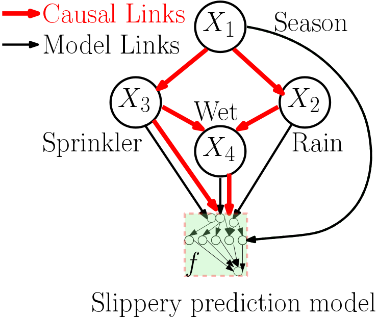
Figure 1: Causal graph for the sprinkler example from Chapter 1.2 of Pearl, (2009). The model, $f$, can be expanded into its own graph. To simplify the exposition, although $f$ takes $4$ variables as input, we arbitrarily assumed that it only depends on $X_{3}$ and $X_{4}$ directly (i.e., $f(X_{1},X_{2},X_{3},X_{4})=g(X_{3},X_{4})$ for some $g$).

Explaining a model’s predictions by assigning importance to its inputs (i.e., feature attribution) is critical to many applications in which a user interacts with a model to either make decisions or gain a better understanding of a system (Simonyan et al.,, 2013; Lundberg and Lee,, 2017; Zhou et al.,, 2016; Shrikumar et al.,, 2017; Baehrens et al.,, 2010; Binder et al.,, 2016; Springenberg et al.,, 2014; Sundararajan et al.,, 2017; Fisher et al.,, 2018; Breiman,, 2001). However, correlation among input features presents a challenge when estimating feature importance.

Consider a motivating example adapted from Pearl, (2009), in which we are given a model $f$ that takes as input four features: the season of the year ($X_{1}$), whether or not it’s raining ($X_{2}$), whether the sprinkler is on ($X_{3}$), and whether the pavement is wet ($X_{4}$) and outputs a prediction $f(\mathbf{x})$, representing the probability that the pavement is slippery (capital $X$ denotes a random variable; lower case $\mathbf{x}$ denotes a particular sample). Assume, the inputs are related through the causal graph in Figure 1. When assigning feature importance, existing approaches that ignore this causal structure (Janzing et al.,, 2020; Sundararajan and Najmi,, 2019; Datta et al.,, 2016) assign zero importance to the season, since it only indirectly affects the outcome through the other input variables. However, such a conclusion may lead a user astray - since changing $X_{1}$ would most definitely affect the outcome.

Recognizing this limitation, researchers have recently proposed approaches that leverage the causal structure among the input variables when assigning credit (Frye et al.,, 2019; Heskes et al.,, 2020). However, such approaches provide an incomplete picture of a system as they only assign credit to nodes in a graph. For example, the ASV method of Frye et al., (2019) solves the earlier problem of ignoring indirect or upstream effects, but it does so by ignoring direct or downstream effects. In our example, season would get all the credit despite the importance of the other variables. This again may lead a user astray - since intervening on $X_{3}$ or $X_{4}$ would affect the outcome, yet they are given no credit. The Causal Shapley values of Heskes et al., (2020) do assign credit to $X_{3}$ and $X_{4}$, but force this credit to be divided with $X_{1}$. This leads to the problem of features being given less importance simply because their downstream variables are also included in the graph.

Given that current approaches end up ignoring or dividing either downstream (i.e., direct) or upstream (i.e., indirect) effects, we develop Shapley Flow, a comprehensive approach to interpreting a model (or system) that incorporates the causal relationship among input variables, while accounting for both direct and indirect effects. In contrast to prior work, we accomplish this by reformulating the problem as one related to assigning credit to edges in a causal graph, instead of nodes (Figure 2c). Our key contributions are as follows.

• We propose the first (to the best of our knowledge) generalization of Shapley value feature attribution to graphs, providing a complete system-level view of a model.

• Our approach unifies three previous game theoretic approaches to estimating feature importance.

• Through examples on real data, we demonstrate how our approach facilitates understanding feature importance.

In this work, we take an axiomatic approach motivated by cooperative game theory, extending Shapley values to graphs. The resulting algorithm, Shapley Flow, generalizes past work on estimating feature importance (Lundberg and Lee,, 2017; Frye et al.,, 2019; López and Saboya,, 2009). The estimates produced by Shapley Flow represent the unique allocation of credit that conforms to several natural axioms. Applied to real-world systems, Shapley Flow can help a user understand both the direct and indirect impact of changing a variable, generating insights beyond current feature attribution methods.

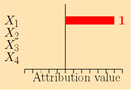
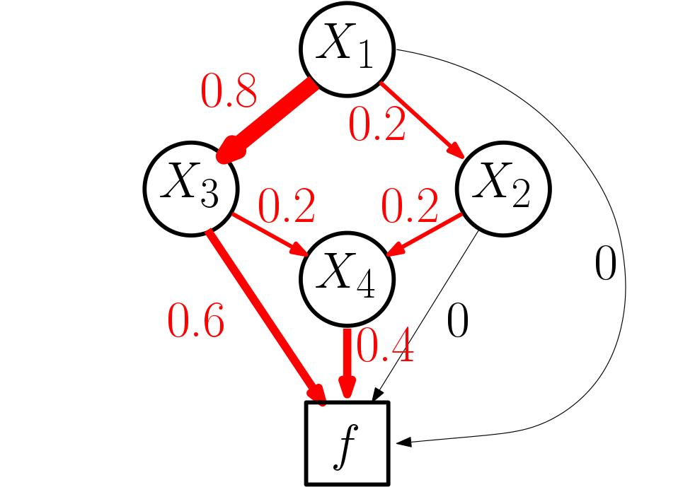
(a) Independent

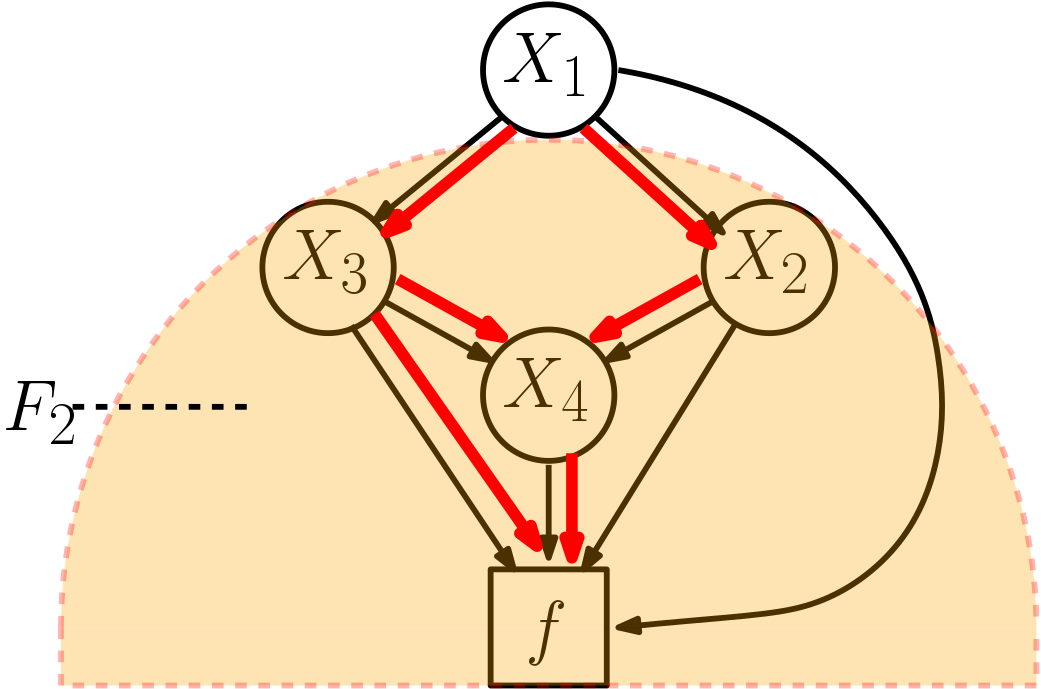
(b) ASV

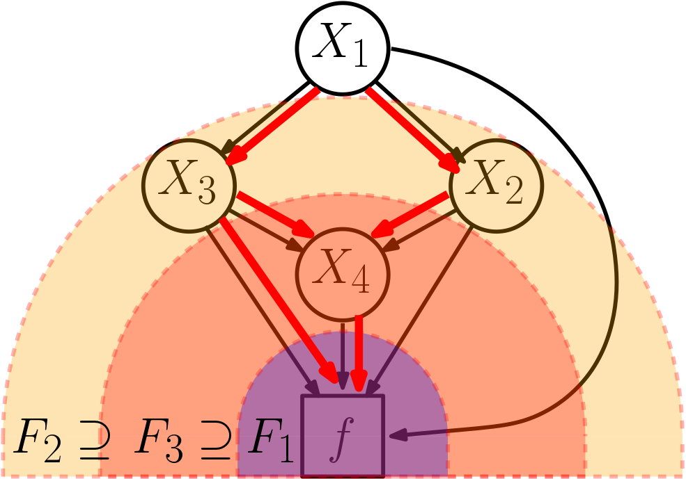
(c) Shapley Flow

Figure 2: Top: Output of attribution methods for the example in Figure 1. Bottom: Causal structure (black edges) and explanation boundaries used by each method. As a reference, we copied the true causal links (red) from Figure 1. An explanation boundary $\mathcal{B}:=(D,F)$ is a cut in the graph that defines a “model” $F$ (nodes in the shaded area in each figure) to be explained. Refer to Section 2.2 for a detailed discussion.

2 Problem Setup & Background

Given a model, or more generally a system, that takes a set of inputs and produces an output, we focus on the problem of quantifying the effect of each input on the output. Here, building off previous work, we formalize the problem setting.

2.1 Problem Setup

Quantifying the effect of each input on a model’s output can be formulated as a credit assignment problem. Formally, given a target sample input $\boldsymbol{x}$, a background sample input $\boldsymbol{x^{\prime}}$, and a model $f:\mathbb{R}^{d}\rightarrow\mathbb{R}$, we aim to explain the difference in output i.e., $f(\boldsymbol{x})-f(\boldsymbol{x^{\prime}})$. We assume $\boldsymbol{x}$ and $\boldsymbol{x}^{\prime}$ are of the same dimension $d$, and each entry can be either discrete or continuous.

We also assume access to a causal graph, as formally defined in Chapter 6 of Peters et al., (2017), over the $d$ input variables. Given this graph, we seek an assignment function $\phi$ that assigns credit $\phi(e)\in\mathbb{R}$ to each edge $e$ in the causal graph such that they collectively explain the difference $f(\boldsymbol{x})-f(\boldsymbol{x^{\prime}})$. In contrast with the classical setting (Lundberg and Lee,, 2017; Sundararajan et al.,, 2017; Frye et al.,, 2020; Aas et al.,, 2019) in which credit is placed on features (ı.e., seeking a node assignment function $\psi(i)\in\mathbb{R}$ for $i\in[1\cdots d]$), our edge-based approach is more flexible because we can recover node $i$’s importance by defining $\psi(i)=\sum_{e\in\text{i's outgoing edges}}\phi(e)$. This exactly matches the classic Shapley axioms (Shapley,, 1953) when the causal graph is degenerate with a single source node connected directly to all the input features.

Here, the effect of the input on the output is measured with respect to a background sample. For example, in a healthcare setting, we may set the features in the background sample to values that are deemed typical for a disease. We assume a single background value for notational convenience, but the formalism easily extends to the common scenario of multiple background values or a distribution of background values, $P$, by defining the explanation target to be $f(\boldsymbol{x})-\mathbb{E}_{\boldsymbol{x^{\prime}}\sim P}f(\boldsymbol{x^{\prime}})$.

2.2 Feature Attribution with a Causal Graph

In our problem setup, we assume access to a causal graph, which can help in reasoning about the relationship among input variable. However, even with a causal graph, feature attribution remains challenging because it is unclear how to rightfully allocate credit for a prediction among the nodes and/or edges of the graph. Marrying interpretation with causality is an active field (see Moraffah et al., (2020) for a survey). A causal graph in and of itself does not solve feature attribution. While a causal graph can be used to answer a specific question with a specific counterfactual, summarizing many counterfactuals to give a comprehensive picture of the model is nontrivial. Furthermore, each node in a causal graph could be a blackbox model that needs to be explained. To address this challenge, we generalize game theoretic fairness principles to graphs.

Given a graph, $\mathcal{G}$, that consists of a causal graph over the the model of interest $f$ and its inputs, we define the boundary of explanation as a cut $\mathcal{B}:=(D,F)$ that partitions the input variables and the output of the model (i.e., the nodes of the graph) into $D$ and $F$ where source nodes (nodes with no incoming edges) are in $D$ and sink nodes (nodes with no outgoing edges) are in $F$. Note that $\mathcal{G}$ has a single sink, $f(\boldsymbol{x})\in\mathbb{R}$. A cut set is the set of edges with one endpoint in $D$ and another endpoint in $F$, denoted as $cut(\mathcal{B})$. It is helpful to think of $F$ as an alternative model definition, where a boundary of explanation (i.e., a model boundary) defines what part of the graph we consider to be the “model”. If we collapse $F$ into a single node that subsumes $f$, then $cut(\mathcal{B})$ represents the direct inputs to this new model.

Depending on the causal graph, multiple boundaries of explanation may exist. Recognizing this multiplicity of choices helps shed light on an ongoing debate in the community regarding feature attribution and whether one should perturb features while staying on the data manifold or perturb them independently (Chen et al.,, 2020; Janzing et al.,, 2020; Sundararajan and Najmi,, 2019). On one side, many argue that perturbing features independently reveals the functional dependence of the model, and is thus true to the model (Janzing et al.,, 2020; Sundararajan and Najmi,, 2019; Datta et al.,, 2016). However, independent perturbation of the data can create unrealistic or invalid sets of model input values. Thus, on the other side, researchers argue that one should perturb features while staying on the data manifold, and so be true to the data (Aas et al.,, 2019; Frye et al.,, 2019). However, this can result in situations in which features not used by the model are given non-zero attribution. Explanation boundaries help us unify these two viewpoints. As illustrated in Figure 2a, when we independently perturb features, we assume the causal graph is flat and the explanation boundary lies between $\boldsymbol{x}$ and $f$ (i.e., $D$ contains all of the input variables). In this example, since features are assumed independent all credit is assigned to the features that directly impact the model output, and indirect effects are ignored (no credit is assigned to $X_{1}$ and $X_{2}$). In contrast, when we perform on-manifold perturbations with a causal structure, as is the case in Asymmetric Shapley Values (ASV) (Frye et al.,, 2019), all the credit is assigned to the source node because the source node determines the value of all nodes in the graph (Figure 2b). This results in a different boundary of explanation, one between the source nodes and the remainder of the graph. Although giving $X_{1}$ credit does not reflect the true functional dependence of $f$, it does for the model defined by $F_{2}$ (Figure 2c). Perturbations that were previously faithful to the data are faithful to a “model”, just one that corresponds to a different boundary. See Section 6 in the Appendix for how on-manifold perturbation (without a causal graph) can be unified using explanation boundaries.

Beyond the boundary directly adjacent to the model of interest, $f$, and the boundary directly adjacent to the source nodes, there are other potential boundaries (Figure 2c) a user may want to consider. However, simply generating explanations for each possible boundary can quickly overwhelm the user (Figures 2a, 2b in the main text, and 8a in the Appendix). Our approach sidesteps the issue of selecting a single explanation boundary by considering all explanation boundaries simultaneously. This is made possible by assigning credit to the edges in a causal graph (Figure 2c). Edge attribution is strictly more powerful than feature attribution because we can simultaneously capture the direct and indirect impact of edges. We note that concurrent work by Heskes et al., (2020) also recognized that existing methods have difficulty capturing the direct and indirect effects simultaneously. Their solution however is node based, so it is forced to split credit between parents and children in the graph.

While other approaches to assign credit on a graph exist, (e.g., Conductance from Dhamdhere et al., (2018) and DeepLift from Shrikumar et al., (2016)), they were proposed in the context of understanding internal nodes of a neural network, and depend on implicit linearity and continuity assumptions about the model. We aim to understand the causal structure among the input nodes in a fully model agnostic manner, where discrete variables are allowed, and no differentiability assumption is made. To do this we generalize the widely used Shapley value (Adadi and Berrada,, 2018; Mittelstadt et al.,, 2019; Lundberg et al.,, 2018; Sundararajan and Najmi,, 2019; Frye et al.,, 2019; Janzing et al.,, 2020; Chen et al.,, 2020) to graphs.

3 Proposed Approach: Shapley Flow

Our proposed approach, Shapley Flow, attributes credit to edges of the causal graph. In this section, we present the intuition behind our approach and then formally show that it uniquely satisfies a generalization of the classic Shapley value axioms, while unifying previously proposed approaches.

3.1 Assigning Credit to Edges: Intuition

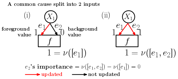
(a) $e_{2}$ updates after $e_{1}$

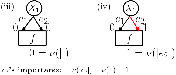
(b) $e_{2}$ updates before $e_{1}$

Figure 3: Edge importance is measured by the change in output when an edge is added. When a model is non-linear, say $f=OR$, we need to average over all scenarios in which $e_{2}$ can be added to gauge its importance. Section 3.1 has a detailed discussion.

Given a causal graph defining the relationship among input variables, we re-frame the problem of feature attribution to focus on the edges of a graph rather than nodes. Our approach results in edge credit assignments as shown in Figure 2c. As mentioned above, this eliminates the need for multiple explanations (i.e., bar charts) pertaining to each explanation boundary. Moreover, it allows a user to better understand the nuances of a system by providing information regarding what would happen if a single causal link breaks.

Shapley Flow is the unique assignment of credit to edges such that a relaxation of the classic Shapley value axioms are satisfied for all possible boundaries of explanation. Specifically, we extend the efficiency, dummy, and linearity axioms from Shapley, (1953) and add a new axiom related to boundary consistency. Efficiency states that the attribution of edges on any boundary must add up to $f(\mathbf{x})-f(\mathbf{x^{\prime}})$. Linearity states that explaining a linear combination of models is the same as explaining each model, and linearly combining the resulting attributions. Dummy states that if adding an edge does not change the output in any scenarios, the edge should be assigned $0$ credit. Boundary consistency states that edges shared by different boundaries need to have the same attribution when explained using either boundary. These concepts are illustrated in Figure 4 and formalized in Section 3.3.

An edge is important if removing it causes a large change in the model’s prediction. However, what does it mean to remove an edge? If we imagine every edge in the graph as a channel that sends its source node’s current value to its target node, then removing an edge $e$ simply means messages sent through $e$ fail. In the context of feature attribution, in which we aim to measure the difference between $f(\mathbf{x})-f(\mathbf{x^{\prime}})$, this means that $e$’s target node still relies on the source’s background value in $\mathbf{x^{\prime}}$ to update its current value, as opposed to the source node’s foreground value in $\mathbf{x}$, as illustrated in Figure 3a. Note that treating edge removal as replacing the parent node with the background value is equivalent to the approach advocated by Janzing et al., (2020), and matches the default behavior of SHAP and related methods. However, we cannot simply toggle edges one at a time. Consider a simple OR function $g(X_{1},X_{2})=X_{1}\vee X_{2}$, with $x_{1}=1$, $x_{2}=1$, $x_{1}^{\prime}=0$, $x_{2}^{\prime}=0$. Removing either of the edges alone, would not affect the output and both $x_{1}$ and $x_{2}$ would be (erroneously) assigned $0$ credit.

To account for this, we consider all scenarios (or partial histories) in which the edge we care about can be added (see Figure 3b). Here, $\nu$ is a function that takes a list of edges and evaluates the network with edges updated in the order specified by the list. For example, $\nu([e_{1}])$ corresponds to the evaluation of $f$ when only $e_{1}$ is updated. Similarly $\nu([e_{1},e_{2}])$ is the evaluation of $f$ when $e_{1}$ is updated followed by $e_{2}$. The list $[e_{1},e_{2}]$ is also referred to as a (complete) history as it specifies how $\mathbf{x^{\prime}}$ changes to $\mathbf{x}$.

For the same edge, attributions derived from different explanation boundaries should agree, otherwise simply including more details of a model in the causal graph would change upstream credit allocation, even though the model implementation was unchanged. We refer to this property as boundary consistency. The Shapley Flow value for an edge is the difference in model output when removing the edge averaged over all histories that are boundary consistent (as defined below).

3.2 Model explanation as value assignments in games

The concept of Shapley value stems from game theory, and has been extensively applied in model interpretability (Štrumbelj and Kononenko,, 2014; Datta et al.,, 2016; Lundberg and Lee,, 2017; Frye et al.,, 2019; Janzing et al.,, 2020). Before we formally extend it to the context of graphs, we define the credit assignment problem from a game theoretic perspective.

Given the message passing system in Section 3.1, we formulate the credit assignment problem as a game specific to an explanation boundary $\mathcal{B}:=(D,F)$. The game consists of a set of players $\mathcal{P}_{\mathcal{B}}$, and a payoff function $\nu_{\mathcal{B}}$. We model each edge external to $F$ as a player. A history is a list of edges detailing the event from $t=0$ (values being $\mathbf{x^{\prime}}$) to $t=T$ (values being $\mathbf{x}$). For example, the history $[i,j,i]$ means that the edge $i$ finishes transmitting a message containing its source node’s most recent value to its target node, followed by the edge $j$, and followed by the edge $i$ again. A coalition is a partial history from $t=0$ to any $t\in[0\cdots T]$. The payoff function, $\nu$, associates each coalition with a real number, and is defined in our case as the evaluation of $F$ following the coalition.

This setup is a generalization of a typical cooperative game in which the ordering of players does not matter (only the set of players matters). However, given our message passing system, history is important. In the following sections, we denote ‘$+$’ as list concatenation, ‘$[]$’ as an empty coalition, and $\mathcal{H}_{\mathcal{B}}$ as the set of all possible histories. We denote $\tilde{\mathcal{H}}_{\mathcal{B}}\subseteq\mathcal{H}_{\mathcal{B}}$ as the set of boundary consistent histories. The corresponding coalitions for $\mathcal{H}_{\mathcal{B}}$ and $\tilde{\mathcal{H}}_{\mathcal{B}}$ are denoted as $\mathcal{C}_{\mathcal{B}}$ and $\tilde{\mathcal{C}}_{\mathcal{B}}$ respectively. A sample game setup is illustrated in Figure 3.

3.3 Axioms

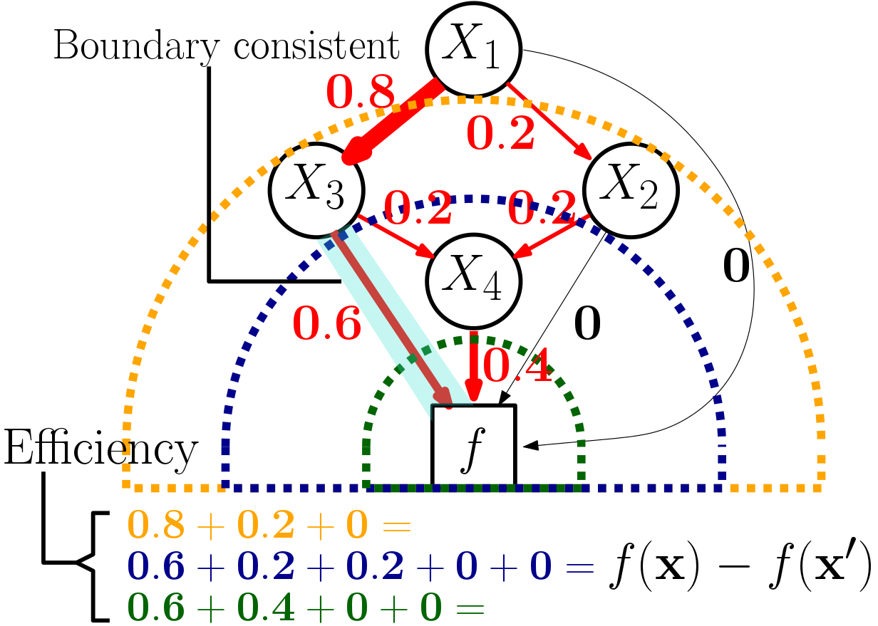
(a) Effi. $+$ Bound. Consist.

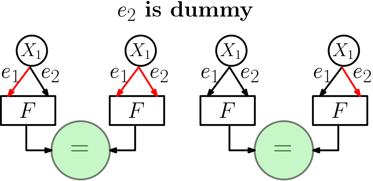
(b) Dummy player

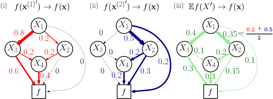
(c) Linearity

Figure 4: Illustration for axioms for Shapley Flow. Except for boundary consistency, all axioms stem from Shapley value’s axioms (Shapley,, 1953). Detailed explanations are included in Section 3.3.

We formally extend the classic Shapley value axioms (efficiency, linearity, and dummy) and include one additional axiom, the boundary consistency axiom, that connects all boundaries together.

• Boundary consistency: for any two boundaries $\mathcal{B}_{1}=(D_{1},F_{1})$ and $\mathcal{B}_{2}=(D_{2},F_{2})$, $\phi_{\nu_{\mathcal{B}_{1}}}(i)=\phi_{\nu_{\mathcal{B}_{2}}}(i)$ for $i\in cut(\mathcal{B}_{1})\cap cut(\mathcal{B}_{2})$

  For edges that are shared between boundaries, their attributions must agree. In Figure 4a, the edge wrapped by a teal band is shared by both the blue and green boundaries, forcing them to give the same attribution to the edge.

In the general setting, not all credit assignments are boundary consistent; different boundaries could result in different attributions for the same edge. This occurs when histories associated with different boundaries are inconsistent (Figure 5). Moving the boundary from $\mathcal{B}$ to $\mathcal{B}^{*}$ (where $\mathcal{B}^{*}$ is the boundary with $D$ containing $f$’s inputs), results in a more detailed set of histories. This expansion has $2$ constraints. First, any history in the expanded set follows the message passing system in Section 3.1. Second, when a message passes through the boundary, it immediately reaches the end of computation as $F$ is assumed to be a black-box.

Denoting the history expansion function into $\mathcal{B}^{*}$ as $HE$ (i.e., $HE$ takes a history $h$ as input and expand it into a set of histories in $\mathcal{B}^{*}$ as output) and denoting the set of all boundaries as $\mathcal{M}$, a history $h$ is boundary consistent if $\exists h_{\mathcal{B}}\in\mathcal{H}_{\mathcal{B}}$ for all $\mathcal{B}\in\mathcal{M}$ such that

$$(\bigcap_{\mathcal{B}\in\mathcal{M}}HE(h_{\mathcal{B}}))\cap HE(h)\neq\emptyset$$

That is $h$ needs to have at least one fully detailed history in which all boundaries can agree on. $\tilde{\mathcal{H}}$ is all histories in $\mathcal{H}$ that are boundary consistent. We rely on this notion of boundary consistency in generalizing the Shapley axioms to any explanation boundary, $\mathcal{B}$:

• Efficiency: $\sum_{i\in cut(\mathcal{B})}\phi_{\nu_{\mathcal{B}}}(i)=f(\mathbf{x})-f(\mathbf{x^{\prime}})$.

  In the general case where $\nu_{\mathcal{B}}$ can depend on the ordering of $h$, the sum is $\sum_{h\in\tilde{\mathcal{H}}_{\mathcal{B}}}\frac{\nu_{\mathcal{B}}(h)}{|\tilde{\mathcal{H}}_{\mathcal{B}}|}-\nu_{\mathcal{B}}([])$. But when the game is defined by a model function $f$, $\sum_{h\in\tilde{\mathcal{H}}_{\mathcal{B}}}\nu_{\mathcal{B}}(h)/|\tilde{\mathcal{H}}_{\mathcal{B}}|=f(\boldsymbol{x})$ and $\nu_{\mathcal{B}}([])=f(\boldsymbol{x^{\prime}})$. An illustration with $3$ boundaries is shown in Figure 4a.

• Linearity: $\phi_{\alpha u+\beta v}=\alpha\phi_{u}+\beta\phi_{v}$ for any payoff functions $u$ and $v$ and scalars $\alpha$ and $\beta$.

  Linearity enables us to compute a linear ensemble of models by independently explaining each model and then linearly weighting the attributions. Similarly, we can explain $f(\mathbf{x})-\mathbb{E}(f(X^{\prime}))$ by independently computing attributions for each background sample $\mathbf{x^{(i)^{\prime}}}$ and then taking the average of the attributions, without recomputing from scratch whenever the background sample’s distribution changes. An illustration with $2$ background samples is shown in Figure 4c.

• Dummy player: $\phi_{\nu_{\mathcal{B}}}(i)=0$ if $\nu_{\mathcal{B}}(S+[i])=\nu_{\mathcal{B}}(S)$ for all $S,S+[i]\in\tilde{\mathcal{C}}_{\mathcal{B}}$ for $i\in cut(\mathcal{B})$.

  Dummy player states that if an edge does not change the model’s output when added to in all possible coalitions, it should be given $0$ attribution. In Figure 4b, $e_{2}$ is a dummy edge because starting from any coalition, adding $e_{2}$ wouldn’t change the output.

These last three axioms are extensions of Shapley’s axioms. Note that Shapley value also requires the symmetry axiom because the game is defined on a set of players. For Shapley Flow values this symmetry assumption is encoded through our choice of an ordered history formulation. (Appendix Section 8).

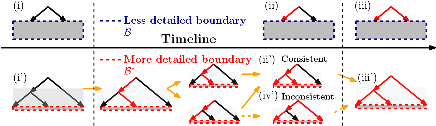
Figure 5: Boundary Consistency. For the blue boundary (upper), we show one potential history $h$. When we expand $h$ to the red boundary (lower), $h$ corresponds to multiple histories as long as each history contains states that match (i) (ii) and (iii). (i’) matches (i), no messages are received in both states. (ii’) matches (ii), the full impact of message transmitted through the left edge is received at the end of computation. (iii’) matches (iii), all messages are received. In contrast, the history containing (iv’) has no state matching (ii), and thus is inconsistent with $h$.

3.4 Shapley Flow is the unique solution

Shapley Flow uniquely satisfies all axioms from the previous section. Here, we describe the algorithm, show its formulae, and state its properties. Please refer to Appendix 7 and 8 for the pseudo code and proof.

Description: Define a configuration of a graph as an arbitrary ordering of outgoing edges of a node when it is traversed by depth first search. For each configuration, we run depth first search starting from the source node, processing edges in the order of the configuration. When processing an edge, we update the value of the edge’s target node by making the edge’s source node value visible to its function. If the edge’s target node is the sink node, the difference in the sink node’s output is credited to every edge along the search path from source to sink. The final result averages over attributions for all configurations.

Formulae: Denote the attribution of Shapley Flow to a path as $\tilde{\phi}_{\nu}$, and the set of all possible orderings of source nodes to a sink path generated by depth first search (DFS) as $\Pi_{\text{dfs}}$. For each ordering $\pi\in\Pi_{\text{dfs}}$, the inequality of $\pi(j)<\pi(i)$ denotes that path $j$ precedes path $i$ under $\pi$. Since $\nu$’s input is a list of edges, we define $\tilde{\nu}$ to work on a list of paths. The evaluation of $\tilde{\nu}$ on a list of paths is the value of $v$ evaluated on the corresponding edge traversal ordering. Then

$$\tilde{\phi}_{\nu}(i)=\sum_{\pi\in\Pi_{\text{dfs}}}\frac{\tilde{\nu}([j:\pi(j)\leq\pi(i)])-\tilde{\nu}([j:\pi(j)<\pi(i)])}{|\Pi_{\text{dfs}}|}$$ (1)

To obtain an edge $e$’s attribution $\phi_{v}(e)$, we sum the path attributions for all paths that contains $e$.

$$\phi_{\nu}(e)=\sum_{p\in\text{paths in }\mathcal{G}}\mathds{1}_{p\text{ contains}}(e)\tilde{\phi}_{\nu}(p)$$ (2)

Additional properties: Shapley Flow has the following beneficial properties beyond the axioms.

Generalization of SHAP: if the graph is flat, the edge attribution is equal to feature attribution from SHAP because each input node is paired with a single edge leading to the model.

Generalization of ASV: the attribution to the source nodes is the same as in ASV if all the dependencies among features are modeled by the causal graph.

Generalization of Owen value: if the graph is a tree, the edge attribution for incoming edges to the leaf nodes is the Owen value (López and Saboya,, 2009) with a coalition structure defined by the tree.

Implementation invariance: implementation invariance means that no matter how the function is implemented, so long as the input and output remain unchanged, so does the attribution (Sundararajan et al.,, 2017), which directly follows boundary consistency (i.e., knowing $f$’s computational graph or not wouldn’t change the upstream attribution).

Conservation of flow: efficiency and boundary consistency imply that the sum of attributions on a node’s incoming edges equals the sum of its outgoing edges.

Model agnostic: Shapley Flow can explain arbitrary (non-differentiable) machine learning pipelines.

4 Practical Application

Shapley Flow highlights both the direct and indirect impact of features. In this section, we consider several applications of Shapley Flow. First, in the context of a linear model, we verify that the attributions match our intuition. Second, we show how current feature attribution approaches lead to an incomplete understanding of a system compared to Shapley Flow.

4.1 Experimental Setup

We illustrate the application of Shapley Flow to a synthetic and a real dataset. In addition, we include results for a third dataset in the Appendix. Note that our algorithm assumes a causal graph is provided as input. In recent years there has been significant progress in causal graph estimation (Glymour et al.,, 2019; Peters et al.,, 2017). However, since our focus is not on causal inference, we make simplifying assumptions in estimating the causal graphs (see Section 9.2 of the Appendix for details).

Datasets. Synthetic: As a sanity check, we first experiment with synthetic data. We create a random graph dataset with $10$ nodes. A node $i$ is randomly connected to node $j$ (with $j$ pointing to $i$) with $0.5$ probability if $i>j$, otherwise $0$. The function at each node is linear with weights generated from a standard normal distribution. Sources follow a $N(0,1)$ distribution. This results in a graph with a single sink node associated with function $f$ (i.e., the ‘model’ of interest). The remainder of the graph corresponds to the causal structure among the input variables.

National Health and Nutrition Examination Survey: This dataset consists of $9,932$ individuals with $18$ demographic and laboratory measurements (Cox,, 1998). We used the same preprocessing as described by Lundberg et al., (2020). Given these inputs, the model, $f$, aims to predict survival.

Model training. We train $f$ using an $80/20$ random train/test split. For experiments with linear models, $f$ is trained with linear regression. For experiments with non-linear models, $f$ is fitted by $100$ XGBoost trees with a max depth of $3$ for up to $1000$ epochs, using the Cox loss.

Causal Graph. For the nutrition dataset, we constructed a causal graph (Figure 9a) based on our limited understanding of the causal relationship among input variables. This graph represents an oversimplification of the true underlying causal relationships and is for illustration purposes only. We assigned attributes predetermined at birth (age, race, and sex) as source nodes because they temporally precede all other features. Poverty index depends on age, race, and sex (among other variables captured by the poverty index noise variable) and impacts one’s health. Other features pertaining to health depend on age, race, sex, and poverty index. Note that the relationship among some features is deterministic. For example, pulse pressure is the difference between systolic and diastolic blood pressure. We include causal edges to account for such facts. We also account for when features have natural groupings. For example, transferrin saturation (TS), total iron binding capacity (TIBC), and serum iron are all related to blood iron. Serum albumin and serum protein are both blood protein measures. Systolic and diastolic blood pressure can be grouped into blood pressure. Sedimentation rate and white blood cell counts both measure inflammation. We add these higher level grouping concepts as new latent variables in the graph. To account for noise in modeling the outcome (i.e., the effect of exogenous variables that are not used as input to the model), we add an independent noise node to each node (detailed in Section 9.2 in the Appendix). The resulting causal structure is an oversimplification of the true causal structure; the relationship between source nodes (e.g., race) and biomarkers is far more complex (Robinson et al.,, 2020). Nonetheless, it can help in understanding the in/direct effects of input variables on the outcome.

4.2 Baselines

We compare Shapley Flow with other game theoretic feature attribution methods: independent SHAP (Lundberg and Lee,, 2017), on-manifold SHAP (Aas et al.,, 2019), and ASV (Frye et al.,, 2019), covering both independent and on-manifold feature attribution.

Since Shapley value based methods are expensive to compute exactly, we use a Monte Carlo approximation of Equation 1. In particular, we sample orderings from $\Pi_{\text{dfs}}$ and average across those orderings.We randomly selected a background sample from each dataset and share it across methods so that each uses the same background. A single background sample allows us to ignore differences in methods due to variations in background sampling and is easier to explain the behavior of baselines (Merrick and Taly,, 2020). To show that our result is not dependent on the particular choice of background sample, we include an example averaged over $100$ background samples in Section 10.4 in the Appendix (the qualitative results shown with a single background still holds). We sample $10,000$ orderings from each approach to generate the results. Since there’s no publicly available implementation for ASV, we show the attribution for source nodes (the noise node associated with each feature) obtained from Shapley Flow (summing attributions of outgoing edges), as they are equivalent given the same causal graph. Since noise node’s credit is used, intermediate nodes can report non zero credit in ASV.

For convenience of visual inspection, we show top $10$ links used by Shapley Flow (credit measured in absolute value) on the nutrition dataset.

4.3 Sanity checks with linear models

To build intuition, we first examine linear models (i.e., $f(\mathbf{x})=\mathbf{w}^{\top}\mathbf{x}+b$ where $\mathbf{w}\in\mathbb{R}^{d}$ and $b\in\mathbb{R}$; the causal dependence inside the graph is also linear). When using a linear model the ground truth direct impact of changing feature $X_{i}$ is $w_{i}(x_{i}-x_{i}^{\prime})$ (that is the change in output due to $X_{i}$ directly), and the ground truth indirect impact is defined as the change in output when an intervention changes $x_{i}^{\prime}$ to $x_{i}$. Note that when the model is linear, only $1$ Monte Carlo sample is sufficient to recover the exact attribution because feature ordering doesn’t matter (the output function is linear in any boundary edges, thus only the background and foreground value of a feature matters). This allows us to bypass sampling errors and focus on analyzing the algorithms.

Results for explaining the datasets are included in Table 1. We report the mean absolute error (and its variance) associated with the estimated attribution (compared against the ground truth attribution), averaged across $1,000$ randomly selected test examples and all graph nodes for both datasets. Note that only Shapley flow results in no error for both direct and indirect effects.

Methods	Nutrition (D)	Synthetic (D)	Nutrition (I)	Synthetic (I)
Independent	0.0 ($\pm$ 0.0)	0.0 ($\pm$ 0.0)	0.8 ($\pm$ 2.7)	1.1 ($\pm$ 1.4)
On-manifold	1.3 ($\pm$ 2.5)	0.8 ($\pm$ 0.7)	0.9 ($\pm$ 1.6)	1.5 ($\pm$ 1.5)
ASV	1.5 ($\pm$ 3.3)	1.2 ($\pm$ 1.4)	0.6 ($\pm$ 1.9)	1.1 ($\pm$ 1.5)
Shapley Flow	0.0 ($\pm$ 0.0)	0.0 ($\pm$ 0.0)	0.0 ($\pm$ 0.0)	0.0 ($\pm$ 0.0)

Table 1: Mean absolute error (std) for all methods on direct (D) and indirect (I) effect for linear models. Shapley Flow makes no mistake across the board.

4.4 Examples with non-linear models

We demonstrate the benefits of Shapley Flow with non-linear models containing both discrete and continuous variables. As a reminder, the baseline methods are not competing with Shapley Flow as the latter can recover all the baselines given the corresponding causal structure (Figure 2). Instead, we highlight why a holistic understanding of the system is better.

Independent SHAP ignores the indirect impact of features. Take an example from the nutrition dataset (Figure 6). Independent SHAP gives lower attribution to age compared to ASV. This happens because age, in addition to its direct impact, indirectly affects the output through blood pressure, as shown by Shapley Flow (Figure 6a). Independent SHAP fails to account for the indirect impact of age, leaving the user with a potentially misleading impression that age is less important than it actually is.

On-manifold SHAP provides a misleading interpretation. With the same example (Figure 6), we observe that on-manifold SHAP strongly disagrees with independent SHAP, ASV, and Shapley Flow on the importance of age. Not only does it assign more credit to age, it also flips the sign, suggesting that age is protective. However, Figure 7a shows that age and earlier mortality are positively correlated; then how could age be protective? Figure 7b provides an explanation. Since SHAP considers all partial histories regardless of the causal structure, when we focus on serum magnesium and age, there are two cases: serum magnesium updates before or after age. We focus on the first case because it is where on-manifold SHAP differs from other baselines (all baselines already consider the second case as it satisfies the causal ordering). When serum magnesium updates before age, the expected age given serum magnesium is higher than the foreground age (yellow line above the black marker). Therefore when age updates to its foreground value, we observe a decrease in age, leading to a decrease in the output (so age appears to be protective). From both an in/direct impact perspective, on-manifold perturbation can be misleading since it is based not on causal but on observational relationships.

ASV ignores the direct impact of features. As shown in Figure 6, serum protein appears to be more important in independent SHAP compared to ASV. From Shapley Flow (Figure 6a), we know serum protein is not given attribution in ASV because its upstream node, blood protein, gets all the credit. However, looking at ASV alone, one fails to understand that intervening on serum protein could have a larger impact on the output.

Shapley Flow shows both direct and indirect impacts of features. Focusing on the attribution given by Shapley Flow (Figure 6a). We not only observe similar direct impacts in variables compared to independent SHAP, but also can trace those impacts to their source nodes, similar to ASV. Furthermore, Shapley Flow provides more detail compared to other approaches. For example, using Shapley Flow we gain a better understanding of the ways in which age impacts survival. The same goes for all other features. This is useful because causal links can change (or break) over time. Our method provides a way to reason through the impact of such a change.

Top features	Age	Serum Magnesium	Serum Protein
Background sample	35	1.37	7.6
Foreground sample	40	1.19	6.5

Attributions	Independent	On-manifold	ASV
Age	0.1	-0.26	0.16
Serum Magnesium	0.02	0.2	0.02
Serum Protein	-0.09	0.07	0.0
Blood pressure	0.0	0.0	-0.14
Systolic BP	-0.05	-0.05	0.0
Diastolic BP	-0.04	-0.07	0.0
Serum Cholesterol	0.0	-0.15	0.0
Serum Albumin	0.0	-0.14	0.0
Blood protein	0.0	0.0	-0.08
White blood cells	0.0	0.11	0.0
Race	0.0	0.09	0.0
BMI	-0.0	0.08	-0.0
TIBC	0.0	0.06	0.0
Sex	0.0	-0.05	0.0
TS	0.0	0.05	0.0
Pulse pressure	0.0	-0.05	0.0
Poverty index	0.0	0.04	0.0
Red blood cells	0.0	0.03	0.0
Serum Iron	0.0	-0.02	0.0
Sedimentation rate	0.0	0.0	0.0
Iron	0.0	0.0	-0.0
Inflamation	0.0	0.0	0.0

(a) Shapley Flow

Figure 6: Comparison among baselines on a sample (top table) from the nutrition dataset, showing top 10 features/edges.

(a) Age vs. output

(b) Age vs. magnesium

Figure 7: Age appears to be protective in on-manifold SHAP because it steals credit from other variables.

More case studies with an additional dataset are included in the Appendix.

5 Discussion and Conclusion

We extend the classic Shapley value axioms to causal graphs, resulting in a unique edge attribution method: Shapley Flow. It unifies three previous Shapley value based feature attribution methods, and enables the joint understanding of both the direct and indirect impact of features. This more comprehensive understanding is useful when interpreting any machine learning model, both ‘black box’ methods, and ‘interpretable’ methods (such as linear models).

The key message of the paper is that model interpretation methods should include the whole machine learning pipeline in order to understand when a model can be applied. While our approach relies on access to a complete causal graph, Shapley Flow is still valuable because a) there are well-established causal relationships in domains such as healthcare, and ignoring such relationships can produce confusing explanations; b) recent advancements in causal estimation are complementary to our work and make defining these graphs easier; c) finally and most importantly, existing methods already implicitly make causal assumptions, Shapley Flow just makes these assumptions explicit (Figure 2). However, this does open up new research opportunities. Can Shapley Flow work with partially defined causal graphs? How to explore Shapley Flow attribution when the causal graph is complex? Can Shapley Flow be useful for feature selection? We leave those questions for future work.

6 Explanation boundary for on-manifold methods without a causal graph

(a) On-manifold attribution

(b) On-manifold boundary

Figure 8: On manifold perturbation methods can be computed using Shapley Flow with a specific explanation boundary.

On-manifold perturbation using conditional expectations can be unified with Shapley Flow using explanation boundaries (Figure 8a). Here we introduce $\tilde{X_{i}}$ as an auxiliary variable that represent the imputed version of $X_{i}$. Perturbing any feature $X_{i}$ affects all input to the model ($\tilde{X_{1}}$, $\tilde{X_{2}}$, $\tilde{X_{3}}$, $\tilde{X_{4}}$) so that they respect the correlation in the data after the perturbation. When $X_{i}$ has not been perturbed, $\tilde{X}_{j}$ treats it as missing for $i,j\in[1,2,3,4]$ and would sample $\tilde{X}_{j}$ from the conditional distribution of $X_{j}$ given non-missing predecessors. The red edges contain causal links from Figure 1, whereas the black edges are the causal structure used by the on-manifold perturbation method. The credit is equally split among the features because they are all correlated. Again, although giving $X_{1}$ and $X_{2}$ credit is not true to $f$, it is true to the model defined by $F$.

7 The Shapley Flow algorithm

A pseudo code implementation highlighting the main ideas for Shapley Flow is included in Algorithm 1. For approximations, instead of trying all edge orderings in line $15$ of Algorithm 1, one can try random orderings and average over the number of orderings tried.

Algorithm 1 Shapley Flow pseudo code

Input: A computational graph $\mathcal{G}$ (each node $i$ has a function $f_{i}$), foreground sample $\mathbf{x}$, background sample $\mathbf{x^{\prime}}$
Output: Edge attribution $\phi:E\rightarrow\mathbb{R}$
Initialization:
$\mathcal{G}$: add an new source node pointing to original source nodes.

1:function ShapleyFlow($\mathcal{G}$, $\mathbf{x}^{\prime}$, $\mathbf{x}$)

2:     Initialize($\mathcal{G}$, $\mathbf{x}^{\prime}$, $\mathbf{x}$) $\triangleright$ Set up game $\nu$ for any boundary in $\mathcal{G}$

3:     $s$ $\leftarrow$ source($\mathcal{G}$) $\triangleright$ Obtain the source node

4:     return DFS($s$, $\{\}$, $[]$)

5:end function

6:

7:function DFS($s$, $D$, $S$)

8:     $\triangleright$ $s$ is a node, $D$ is the data side of the current boundary, $S$ is coalition

9:     $\triangleright$ Using Python list slice notation

10:     Initialize $\phi$ to output $0$ for all edges

11:     if IsSinkNode(s) then

12:         $\triangleright$ Here we overload $D$ to refer to its boundary

13:         $\phi(S[-1])$ $\leftarrow$ $\nu_{D}(S)-\nu_{D}(S[:-1])$ $\triangleright$ Difference in output is attributed to the edge

14:         return $\phi$

15:     end if

16:

17:     for $p\leftarrow\text{AllOrderings}(\text{Children}(s))$ do $\triangleright$ Try all orderings/permutations of the node’s children

18:         for $c\leftarrow p$ do $\triangleright$ Follow the permutation to get the node one by one

19:              edgeCredit $\leftarrow$ DFS($c$, $D\cup\{s\}$, $S+[(s,c)]$) $\triangleright$ Recurse downward

20:

21:              $\phi$ $\leftarrow$ $\phi+\frac{\text{edgeCredit}}{\text{NumChildren}(s)!}$ $\triangleright$ Average attribution over number of runs

22:              $\phi(S[-1])$ $\leftarrow$ $\phi(S[-1])+\frac{\text{edgeCredit}(s,c)}{\text{NumChildren}(s)!}$ $\triangleright$ Propagate upward

23:         end for

24:     end for

25:     return $\phi$

26:end function

8 Shapley Flow’s uniqueness proof

Without loss of generality, we can assume $\mathcal{G}$ has a single source node $s$. We can do this because every node in a causal graph is associated with an independent noise node (Peters et al.,, 2017, Chapter 6). For deterministic relationships, the function for a node doesn’t depend on its noise. Treating those noise nodes as a single node, $s$, wouldn’t have changed any boundaries that already exist in the original graph. Therefore we can assume there is a single source node $s$.

8.1 At most one solution satisfies the axioms

Assuming that a solution exists, we show that it must be unique.

Proof.

We adapt the argument from the Shapley value uniqueness proof , by defining basis payoff functions as carrier games. Choose any boundary $\mathcal{B}$, we show here that any game defined on the boundary has a unique attribution. We also drop the subscript $\mathcal{B}$ in the proof as there is no ambiguity. Note that since every edge will appear in some boundary, if all boundary edges are uniquely attributed to, all edges have unique attributions. A carrier game associated with coalition (ordered list) $O$ is a game with payoff function $v^{O}$ such that $v^{O}(S)=1(0)$ if coalition $S$ starts with $O$ (otherwise 0). By dummy player, we know that only the last edge $e$ in $O$ gets credit and all other edges in the cut set are dummy because a coalition is constructed in order (only adding $e$ changes the payoff from $0$ to $1$). Note that in contrast with the traditional symmetry axiom (Shapley,, 1953) defined on a set of players, the symmetry axiom is not explicit in our case (it is made implicitly) because not all edges in the carrier game are symmetric with each other (observe that $e$ is different from all other edges, which are dummy), thus we do not need an explicit symmetry axiom to argue for unique attribution in the carrier game. Furthermore, $e$ must be an edge in the boundary to form a valid game because boundary edges are the only edges that are connected to the model defined by the boundary. Therefore we give $0$ credit to edges in the cut set other than $e$ (because they are dummy players). By the efficiency axiom, we give $\sum_{h\in\tilde{\mathcal{H}}}\frac{\nu_{\mathcal{B}}(h)}{|\tilde{\mathcal{H}}|}-\nu_{\mathcal{B}}([])$ credit to $e$ where $\tilde{\mathcal{H}}$ is the set of all possible boundary consistent histories as defined in Section 3.3. This uniquely attributed the boundary edges for this game.

We show that the set of carrier games associated with every coalition that ends in a boundary edge (denoted as $\hat{\mathcal{C}}$) form basis functions for all payoff functions associated with the system. Recall from Section 3.2 that $\tilde{\mathcal{C}}$ is the set of boundary consistent coalitions. We show here that payoff value on coalitions from $\tilde{\mathcal{C}}$ is redundant given $\hat{\mathcal{C}}$. Note that $\tilde{\mathcal{C}}$ \$\hat{\mathcal{C}}$ represents all the coalitions that do not end in a boundary edge. For $c\in\tilde{\mathcal{C}}$ \$\hat{\mathcal{C}}$, $v^{O}(c)=v^{O}(c[:-1])$ (using Python’s slice notation on list) because only boundary edges are connected to the model defined by the boundary. Therefore it suffices to show that $v^{O}$ is linearly independent for $O\in\hat{\mathcal{C}}$. For a contradiction, assume for all $c\in\hat{\mathcal{C}}$, $\sum_{O\subseteq\hat{\mathcal{C}}}\alpha^{O}v^{O}(c)=0$, with some non zero $\alpha^{O}\in\mathbb{R}$ (definition of linear dependence). Let $S$ be a coalition with minimal length such that $\alpha^{S}\neq 0$. We have $\sum_{O\subseteq\hat{\mathcal{C}}}\alpha^{O}v^{O}(S)=\alpha^{S}$, a contradiction.

Therefore for any $\nu$ we have unique $\alpha$’s such that $\nu=\sum_{O\subseteq\hat{\mathcal{C}}}\alpha^{O}v^{O}$. Using the linearity axiom, we have

$$\phi_{\nu}=\phi_{\sum_{O\subseteq\hat{\mathcal{C}}}\alpha^{O}v^{O}}=\sum_{O\subseteq\hat{\mathcal{C}}}\alpha^{O}\phi_{v^{O}}$$

The uniqueness of $\alpha$ and $\phi_{v^{O}}$ makes the attribution unique if a solution exists. Axioms used in the proof are italicized.

∎

8.2 Shapley Flow satisfies the axioms

Proof.

We first demonstrate how to generate all boundaries. Then we show that Shapley Flow gives boundary consistent attributions. Following that, we look at the set of histories that can be generated by DFS in boundary $\mathcal{B}$, denoted as $\Pi^{\text{dfs}}_{\mathcal{B}}$. We show that $\Pi^{\text{dfs}}_{\mathcal{B}}=\tilde{\mathcal{H}}_{\mathcal{B}}$. Using this fact, we check the axioms one by one.

• Every boundary can be “grown” one node at a time from $D=\{s\}$ where $s$ is the source node: Since the computational graph $\mathcal{G}$ is a directed acyclic graph (DAG), we can obtain a topological ordering of the nodes in $\mathcal{G}$. Starting by including the first node in the ordering (the source node $s$), which defines a boundary as $(D=\{s\},F=\text{Nodes}(\mathcal{G})\backslash D)$, we grow the boundary by adding nodes to $D$ (removing nodes from $F$) one by one following the topological ordering. This ordering ensures the corresponding explanation boundary is valid because the cut set only flows from $D$ to $F$ (if that’s not true, then one of the dependency nodes is not in $D$, which violates topological ordering).

  Now we show every boundary can be “grown” in this fashion. In other words, starting from an arbitrary boundary $\mathcal{B}_{1}=(D_{1},F_{1})$, we can “shrink” one node at a time to $D=\{s\}$ by reversing the growing procedure. First note that, $D_{1}$ must have a node with outgoing edges only pointing to nodes in $F_{1}$ (if that’s not the case, we have a cycle in this graph because we can always choose to go through edges internal to $D_{1}$ and loop indefinitely). Therefore we can just remove that node to arrive at a new boundary (now its incoming edges are in the cut set). By the same argument, we can keep removing nodes until $D=\{s\}$, completing the proof.

• Shapley Flow gives boundary consistent attributions: We show that every boundary grown has edge attribution consistent with the previous boundary. Therefore all boundaries have consistent edge attribution because the boundary formed by any two boundary’s common set of nodes can be grown into those two boundaries using the property above. Let’s focus on the newly added node $c$ from one boundary to the next. Note that a property of depth first search is that every time $c$’s value is updated, its outgoing edges are activated in an atomic way (no other activation of edges occur between the activation of $c$’s outgoing edges). Therefore, the change in output due to the activation of new edges occur together in the view of edges upstream of $c$, thus not changing their attributions. Also, since $c$’s outgoing edges must point to the model defined by the current boundary (otherwise it cannot be a valid topological ordering), they don’t have down stream edges, concluding the proof.

• $\Pi^{\text{dfs}}_{\mathcal{B}}=\tilde{\mathcal{H}}_{\mathcal{B}}$: Since attribution is boundary consistent, we can treat the model as a blackbox and only look at the DFS ordering on the data side. Observe that the edge traversal ordering in DFS is a valid history because a) every edge traversal can be understood as a message received through edge , b) when every message is received, the node’s value is updated, and c) the new node’s value is sent out through every outgoing edge by the recursive call in DFS. Therefore the two side of the equation are at least holding the same type of object.

  We first show that $\Pi^{\text{dfs}}_{\mathcal{B}}\subseteq\tilde{\mathcal{H}}_{\mathcal{B}}$. Take $h\in\Pi^{\text{dfs}}_{\mathcal{B}}$, we need to find a history $h^{*}$ in $\mathcal{B}^{*}$ such that a) $h$ can be expanded into $h^{*}$ and b) for any boundary, there is a history in that boundary that can be expanded into $h^{*}$. Let $h^{*}$ be any history expanded using DFS that is aligned with $h$. To show that every boundary can expand into $h^{*}$, we just need to show that the boundaries generated through the growing process introduced in the first bullet point can be expanded into $h^{*}$. The base case is $D=\{s\}$. There must have an ordering to expand into $h^{*}$ because $h^{*}$ is generated by DFS, and that DFS ensures that every edge’s impact on the boundary is propagated to the end of computation before another edge in $D$ is traversed. Similarly, for the inductive step, when a new node $c$ is added, we just follow the expansion of its previous boundary to reach $h^{*}$.

  Next we show that $\tilde{\mathcal{H}}_{\mathcal{B}}\subseteq\Pi^{\text{dfs}}_{\mathcal{B}}$. First observe that for history $h_{1}$ in $\mathcal{B}_{1}=(D_{1},F_{1})$ and history $h_{2}$ in $\mathcal{B}_{2}=(D_{2},F_{2})$ with $F_{2}\subseteq F_{1}$, if $h_{1}$ cannot be expanded into $h_{2}$, then $HE(h_{1})\cap HE(h_{2})=\emptyset$ because they already have mismatches for histories that doesn’t involve passing through $\mathcal{B}_{1}$. Assume we do have $h\in\tilde{\mathcal{H}}_{\mathcal{B}}$ but $h\not\in\Pi^{\text{dfs}}_{\mathcal{B}}$. To derive a contradiction, we shrink the boundary one node at a time from $\mathcal{B}$, again using the procedure described in the first bullet point. We denote the resulting boundary formed by removing $n$ nodes as $\mathcal{B}_{-n}$. Since $h$ is assumed to be boundary consistent, there exist $h_{\mathcal{B}_{-1}}\in\mathcal{H}_{\mathcal{B}_{-1}}$ such that $h_{\mathcal{B}_{-1}}$ must be able to expand into $h$. Say the two boundaries differ in node $c$. Note that any update to $c$ crosses $\mathcal{B}_{-1}$, therefore its impact must be reached by $F$ before another event occurs in $D_{-1}$. Since all of $c$’s outgoing edges crosses $\mathcal{B}$, any ordering of messages sent through those edges is a DFS ordering from $c$. This means that if $h_{\mathcal{B}_{-1}}$ can be reached by DFS, so can $h_{\mathcal{B}}$, violating the assumption. Therefore, $h_{\mathcal{B}_{-1}}\not\in\Pi^{\text{dfs}}_{\mathcal{B}_{-1}}$ and $h_{\mathcal{B}_{-1}}\in\tilde{\mathcal{H}}_{\mathcal{B}_{-1}}$ (the latter because $h_{\mathcal{B}_{-1}}$ can expand into a history that is consistent with all boundaries by first expanding into $h$). We run the same argument until $D=\{s\}$. This gives a contradiction because in this boundary, all histories can be produced by DFS.

• Efficiency: Since we are attributing credit by the change in the target node’s value following a history $h$ given by DFS, the target for this particular DFS run is thus $\nu_{\mathcal{B}}(h)-\nu_{\mathcal{B}}([])$. Average over all DFS runs and noting that $\tilde{\mathcal{H}}_{\mathcal{B}}=\Pi^{\text{dfs}}_{\mathcal{B}}$ gives the target $\sum_{h\in\tilde{\mathcal{H}}_{\mathcal{B}}}\nu_{\mathcal{B}}(h)/|\tilde{\mathcal{H}}_{\mathcal{B}}|-\nu_{\mathcal{B}}([])$. Noting that each update in the target node’s value must flow through one of the boundary edges. Therefore the sum of boundary edges’ attribution equals to the target.

• Linearity: For two games of the same boundary $v$ and $u$, following any history, the sum of output differences between the two games is the output difference of the sum of the two games, therefore $\phi_{v+u}$ would not differ from $\phi_{v}+\phi_{u}$. It’s easy to see that extending addition to any linear combination wouldn’t matter.

• Dummy player: Since Shapley Flow is boundary consistent, we can just run DFS up to the boundary (treat $F$ as a blackbox). Since every step in DFS remains in the coalition $\tilde{\mathcal{C}}_{\mathcal{B}}$ because $\Pi^{\text{dfs}}_{\mathcal{B}}\subseteq\tilde{\mathcal{H}}_{\mathcal{B}}$, if an edge is dummy, every time it is traversed through by DFS, the output won’t change by definition, thus giving it $0$ credit.

∎

Therefore Shapley Flow uniquely satisfies the axioms. We note that efficiency requirement simplifies to $f(\boldsymbol{x})-f(\boldsymbol{x^{\prime}})$ when applying it to an actual model because all histories from DFS would lead the target node to its target value. We can prove a stronger claim that actually all nodes would reach its target value when DFS finishes. To see that, we do an induction on a topological ordering of the nodes. The source nodes reaches its final value by definition. Assume this holds for the $k^{\text{th}}$ node. For the $k+1^{\text{th}}$ node, its parents achieves target value by induction. Therefore DFS would make the parents’ final values visible to this node, thus updating it to the target value.

9 Causal graphs

While the nutrition dataset is introduced in the main text, we describe an additional dataset to further demonstrate the usefulness of Shapley Flow. Moreover, we describe in detail how the causal relationship is estimated. The resulting causal graphs for the nutrition dataset and the income dataset are visualized in Figure 9.

9.1 The Census Income dataset

The Census Income dataset consists of $32,561$ samples with $12$ features. The task is to predict whether one’s annual income exceeds $50k$. We assume a causal graph, similar to that used by Frye et al., (2019) (Figure 9b). Attributes determined at birth e.g., sex, native country, and race act as source nodes. The remaining features (marital status, education, relationship, occupation, capital gain, work hours per week, capital loss, work class) have fully connected edges pointing from their causal ancestors. All features have a directed edge pointing to the model.

9.2 Causal Effect Estimation

Given the causal structure described above, we estimate the relationship among variables using XGBoost. More specifically, using an $80/20$ train test split, we use XGBoost to learn the function for each node. If the node value is categorical, we train to minimize cross entropy loss. Otherwise, we minimize mean squared error. Models are fitted by $100$ XGBoost trees with a max depth of $3$ for up to $1000$ epochs. Since features are rarely perfectly determined by their dependency node, we add independent noise nodes to account for this effect. That is, each non-sink node is pointed to by a unique noise node that account for the residue effect of the prediction.

Depending on whether the variable is discrete or continuous, we handle the noise differently. For continuous variables, the noise node’s value is the residue between the prediction and the actual value. For discrete variables, we assume the actual value is sampled from the categorical distribution specified by the prediction. Therefore the noise node’s value is any possible random number that could result in the actual value. As a concrete example for handling discrete variable, consider a binary variable $y$, and assume the trained categorical function $f$ gives $f(\boldsymbol{x})=[0.3,0.7]$ where $\boldsymbol{x}$ is the foreground value of the input to predict $y$. We view the data generation as the following. The noise term associated with $y$ is treated as a uniform random variable between $0$ and $1$. If it lands within $0$ to $0.3$, $y$ is sampled to be $0$, otherwise $1$ (matching the categorical function of $70\%$ chance of sampling $y$ to be $1$). Now if we observe the foreground value of $y$ to be $0$, it means the foreground value of noise must be uniform between $0$ to $0.3$. Although we cannot infer the exact value of the noise, we can sample the noise from $0$ to $0.3$ multiple times and average the resulting attribution.

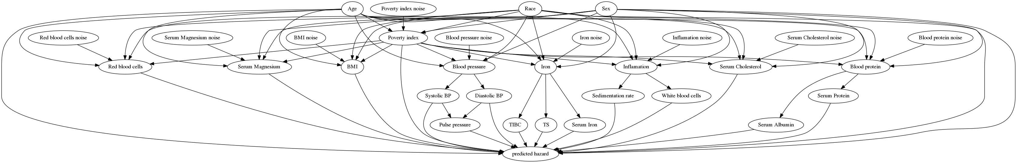
(a) Causal graph for the nutrition dataset

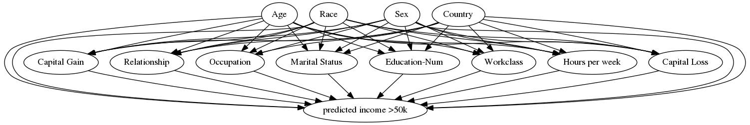
(b) Causal graph for the Census Income dataset

Figure 9: The causal graphs we used for the two real datasets. Note that each node in the causal graph for (a) is given a noise node to account for random effects. The noise nodes are omitted for better readability for (b). The resulting causal structures are over-simplifications of the true causal structure; the relationship between source nodes (e.g., race and sex) and other features is far more complex. They are used as a proof of concept to show both the direct and indirect effect of features on the prediction output.

10 Additional Results

In this section, we first present additional sanity checks with synthetic data. Then we show additional examples from both the nutrition and income datasets to demonstrate how a complete view of boundaries should be preferable over single boundary approaches.

10.1 Additional Sanity Checks

We include further sanity check experiments in this section. The first sanity check consists of a chain with 4 variables. Each node along the chain is an identical copy of its predecessor and the function to explain only depends on $X_{4}$ (Figure 10). The dataset is created by sampling $X_{1}\sim\mathcal{N}(0,1)$, that is a standard normal distribution, with $1000$ samples. We use the first sample as background, and explain the second sample (one can choose arbitrary samples to obtain the same insights). As shown in Figure 10, independent SHAP fails to show the indirect impact of $X_{1}$, $X_{2}$, and $X_{3}$, ASV fails to show the direct impact of $X_{4}$, on manifold SHAP fails to fully capture both the direct and indirect importance of any edge.

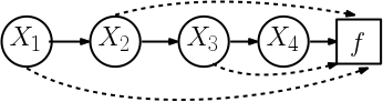
(a) chain dataset

	Independent	On-manifold	ASV
X4	-1.82	-0.45	0.0
X1	0.0	-0.45	-1.82
X3	0.0	-0.45	0.0
X2	0.0	-0.45	0.0

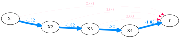
(b) Shapley Flow

Figure 10: (a) The chain dataset contains exact copies of nodes. The dashed edges denotes dummy dependencies. (b) While Shapley Flow shows the entire path of influence, other baselines fails to capture either direct and indirect effects.

Methods	Income	Nutrition	Synthetic
Independent	0.0 ($\pm$ 0.0)	0.0 ($\pm$ 0.0)	0.0 ($\pm$ 0.0)
On-manifold	0.4 ($\pm$ 0.3)	1.3 ($\pm$ 2.5)	0.8 ($\pm$ 0.7)
ASV	0.4 ($\pm$ 0.6)	1.5 ($\pm$ 3.3)	1.2 ($\pm$ 1.4)
Shapley Flow	0.0 ($\pm$ 0.0)	0.0 ($\pm$ 0.0)	0.0 ($\pm$ 0.0)

Table 2: Shapley Flow and independent SHAP have lower mean absolute error (std) for direct effect of features on linear models.

Methods	Income	Nutrition	Synthetic
Independent	0.1 ($\pm$ 0.2)	0.8 ($\pm$ 2.7)	1.1 ($\pm$ 1.4)
On-manifold	0.4 ($\pm$ 0.3)	0.9 ($\pm$ 1.6)	1.5 ($\pm$ 1.5)
ASV	0.1 ($\pm$ 0.1)	0.6 ($\pm$ 1.9)	1.1 ($\pm$ 1.5)
Flow	0.0 ($\pm$ 0.0)	0.0 ($\pm$ 0.0)	0.0 ($\pm$ 0.0)

Table 3: Shapley Flow and ASV have lower mean absolute error (std) for indirect effect on linear models.

The second sanity check consists of linear models as described in Section 4.3. We include the full result with the income dataset added in Table 2 and Table 3 for direct and indirect effects respectively. The trend for the income dataset algins with the nutrition and synthetic dataset: only Shapley Flow makes no mistake for estimating both direct and indirect impact. Independent Shap only does well for direct effect. ASV only does well for indirect effects (it only reaches zero error when evaluated on source nodes).

10.2 Additional examples

In this section, we analyze another example from the nutrition dataset (Figure 11) and 3 additional example from the adult censor dataset.

Independent SHAP ignores the indirect impact of features. Take an example from the nutrition dataset (Figure 11). The race feature is given low attribution with independent SHAP, but high importance in ASV. This happens because race, in addition to its direct impact, indirectly affects the output through blood pressure, serum magnesium, and blood protein, as shown by Shapley Flow (Figure 11a). In particular, race partially accounts for the impact of serum magnesium because changing race from Black to White on average increases serum magnesium by $0.07$ meg/L in the dataset (thus partially explaining the increase in serum magnesium changing from the background sample to the foreground). Independent SHAP fails to account for the indirect impact of race, leaving the user with a potentially misleading impression that race is irrelevant for the prediction.

On-manifold SHAP provides a misleading interpretation. With the same example (Figure 11), we observe that on-manifold SHAP strongly disagrees with independent SHAP, ASV, and Shapley Flow on the importance of age. Not only does it assign more credit to age, it also flips the sign, suggesting that age is protective. However, Figure 12a shows that age and earlier mortality are positively correlated; then how could age be protective? Figure 12b provides an explanation. Since SHAP considers all partial histories regardless of the causal structure, when we focus on serum magnesium and age, there are two cases: serum magnesium updates before or after age. We focus on the first case because it is where on-manifold SHAP differs from other baselines (all baselines already consider the second case as it satisfies the causal ordering). When serum magnesium updates before age, the expected age given serum magnesium is higher than the foreground age (yellow line above the black marker). Therefore when age updates to its foreground value, we observe a decrease in age, leading to a decrease in the output (so age appears to be protective). Serum magnesium is just one variable from which age steals credit. Similar logic applies to TIBC, red blood cells, serum iron, serum protein, serum cholesterol, and diastolic BP. From both an in/direct impact perspective, on-manifold perturbation can be misleading since it is based not on causal but on observational relationships.

ASV ignores the direct impact of features. As shown in Figure 11, serum magnesium appears to be more important in independent SHAP compared to ASV. From Shapley Flow (Figure 11a), this difference is explained by race as its edge to serum magnesium has a negative impact. However, looking at ASV alone, one fails to understand that intervening on serum magnesium could have a larger impact on the output.

Shapley Flow shows both direct and indirect impacts of features. Focusing on the attribution given by Shapley Flow (Figure 11a). We not only observe similar direct impacts in variables compared to independent SHAP, but also can trace those impacts to their source nodes, similar to ASV. Furthermore, Shapley Flow provides more detail compared to other approaches. For example, using Shapley Flow we gain a better understanding of the ways in which race impacts survival. The same goes for all other features. This is useful because causal links can change (or break) over time. Our method provides a way to reason through the impact of such a change.

Top features	Age	Serum Magnesium	Race
Background sample	35.0	1.37	Black
Foreground sample	42.0	1.63	white

Attributions	Independent	On-manifold	ASV
Age	0.23	-0.38	0.3
Serum Magnesium	-0.21	-0.02	-0.15
Race	-0.06	0.04	-0.24
Pulse pressure	0.0	-0.08	0.0
Diastolic BP	0.0	0.08	0.0
Serum Cholesterol	0.0	0.07	0.0
Serum Protein	0.01	0.06	0.0
Serum Iron	0.0	0.05	0.0
Poverty index	-0.02	0.01	-0.01
Systolic BP	-0.03	-0.01	0.0
Red blood cells	0.0	0.05	0.0
Blood protein	0.0	0.0	0.04
TIBC	0.0	0.04	0.0
Blood pressure	0.0	0.0	-0.03
TS	0.0	0.03	0.0
BMI	-0.0	-0.03	-0.0
Sex	0.0	0.02	0.0
Serum Albumin	0.0	-0.01	0.0
White blood cells	0.01	-0.01	0.0
Sedimentation rate	0.0	0.01	0.0
Inflamation	0.0	0.0	0.01
Iron	0.0	0.0	0.0

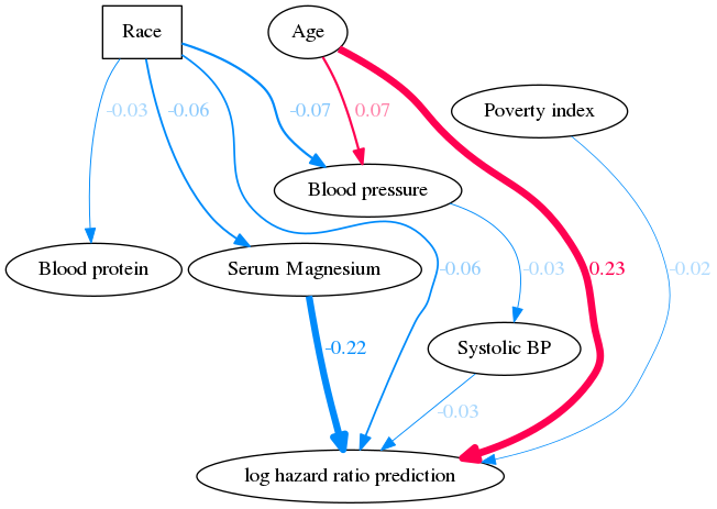
(a) Shapley Flow

Figure 11: Comparison among baselines on a sample (top table) from the nutrition dataset, showing top 10 features/edges. As noted in the main text this graph is an oversimplification and is not necessarily representative of the true underlying causal relationship.

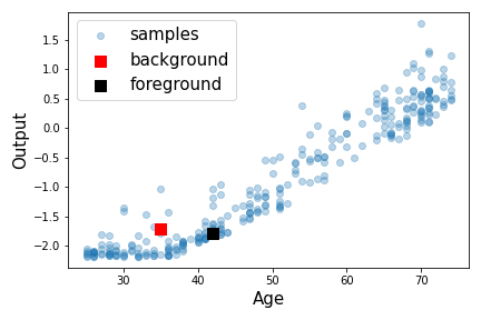
(a) Age vs. output

(b) Age vs. magnesium

Figure 12: Age appears to be protective in on-manifold SHAP because it steals credit from other variables.

Figure 13 gives an example of applying Shapley Flow and baselines on the income dataset. Note that the attribution to capital gain drops from independent SHAP to on-manifold SHAP and ASV. From Shapley Flow, we know the decreased attribution is due to age and race. More examples are shown in Figure 14 and 15.

	Background sample	Foreground sample
Age	39	35
Workclass	State-gov	Federal-gov
Education-Num	13	5
Marital Status	Never-married	Married-civ-spouse
Occupation	Adm-clerical	Farming-fishing
Relationship	Not-in-family	Husband
Race	White	Black
Sex	Male	Male
Capital Gain	2174	0
Capital Loss	0	0
Hours per week	40	40
Country	United-States	United-States

	Independent	On-manifold	ASV
Education-Num	-0.12	-0.11	-0.09
Relationship	0.05	0.06	0.04
Capital Gain	0.09	0.01	0.03
Occupation	-0.03	-0.07	-0.02
Marital Status	0.04	0.05	0.03
Workclass	0.02	0.03	0.02
Race	-0.01	-0.03	0.01
Age	-0.01	-0.01	0.02
Capital Loss	0.0	0.03	0.0
Country	0.0	0.03	0.0
Sex	0.0	0.03	0.0
Hours per week	0.0	0.0	0.0

(a) Shapley Flow

Figure 13: Comparison between independent SHAP, on-manifold SHAP, ASV, and Shapley Flow on a sample from the income dataset. Shapley flow shows the top 10 links. The direct impact of capital gain is not represented by on-manifold SHAP. As noted in the text this graph is based on previous work and is not necessarily representative of the true underlying causal relationship.

	Background sample	foreground sample
Age	39	30
Workclass	State-gov	State-gov
Education-Num	13	13
Marital Status	Never-married	Married-civ-spouse
Occupation	Adm-clerical	Prof-specialty
Relationship	Not-in-family	Husband
Race	White	Asian-Pac-Islander
Sex	Male	Male
Capital Gain	2174	0
Capital Loss	0	0
Hours per week	40	40
Country	United-States	India

	Independent	On-manifold	ASV
Relationship	0.17	0.04	0.13
Capital Gain	0.22	0.01	0.07
Occupation	0.1	0.06	0.07
Marital Status	0.08	0.06	0.07
Country	-0.04	0.07	0.07
Age	-0.0	-0.02	0.13
Education-Num	0.0	0.12	0.0
Race	0.02	0.07	0.0
Workclass	0.0	0.06	0.0
Hours per week	0.0	0.03	0.0
Sex	0.0	0.03	0.0
Capital Loss	0.0	0.01	0.0

(a) Shapley Flow

Figure 14: Comparison between independent SHAP, on-manifold SHAP, ASV, and Shapley Flow on a sample from the income dataset. Shapley flow shows the top 10 links. The indirect impact of age is only highlighted by Shapley Flow and ASV. As noted in the text this graph is based on previous work and is not necessarily representative of the true underlying causal relationship.

	Background sample	Foreground sample
Age	39	30
Workclass	State-gov	Federal-gov
Education-Num	13	10
Marital Status	Never-married	Married-civ-spouse
Occupation	Adm-clerical	Adm-clerical
Relationship	Not-in-family	Own-child
Race	White	White
Sex	Male	Male
Capital Gain	2174	0
Capital Loss	0	0
Hours per week	40	40
Country	United-States	United-States

Attributions	Independent	On-manifold	ASV
Marital Status	0.03	0.08	0.03
Capital Gain	0.06	0.02	0.02
Workclass	0.03	0.03	0.02
Relationship	-0.01	-0.11	0.01
Education-Num	-0.02	0.01	-0.02
Age	-0.02	-0.03	0.01
Country	0.0	0.03	0.0
Capital Loss	0.0	0.03	0.0
Occupation	0.0	-0.03	0.0
Sex	0.0	0.03	0.0
Race	0.0	0.02	0.0
Hours per week	0.0	-0.0	0.0

(a) Shapley Flow

Figure 15: Comparison between independent SHAP, on-manifold SHAP, ASV, and Shapley Flow on a sample from the income dataset. Shapley flow shows the top 10 links. Note that although age appears to be not important for all baselines, its impact through different causal edges are opposite as shown by Shapley Flow.

10.3 A global understanding with Shapley Flow

In addition to explaining a particular example, one can explain an entire dataset with Shapley Flow. Specifically, for multi-class classification problems, we take the average of attributions for the probability predicted for the actual class, in accordance with (Frye et al.,, 2019). A demonstration on the income dataset using $1000$ randomly selected examples is included in Figure 16. As before, we use a single shared background sample for explanation. Here, we observe that although the relative importance across independent SHAP, on-manifold SHAP, and ASV are similar, age and sex have opposite direct versus indirect impact as shown by Shapley Flow.

	Independent	On-manifold	ASV
Capital Gain	0.02	0.02	0.03
Education-Num	0.02	0.03	0.02
Age	0.01	0.01	0.01
Occupation	0.0	0.01	0.0
Capital Loss	0.01	-0.0	0.01
Relationship	0.01	0.0	0.0
Hours per week	0.0	0.01	-0.0
Sex	0.0	-0.01	0.0
Country	0.0	-0.01	0.0
Marital Status	-0.0	0.0	-0.0
Race	0.0	-0.01	-0.0
Workclass	0.0	-0.0	-0.0

(a) Shapley Flow

Figure 16: Comparison of global understanding between independent SHAP, on-manifold SHAP, ASV, and Shapley Flow on the income dataset. Showing only the top $10$ attributions for Shapley Flow for visual clarity.

10.4 Example with multiple background samples

An example with 100 background samples is shown in Figure 17. Shapley Flow shows a holistic picture of feature importance, while other baselines only show part of the picture.

Independent SHAP ignores the indirect impact of features. Take an example from the nutrition dataset (Figure 17). Independent SHAP only considers the direct impact of systolic blood pressure, and ignores its potential impact on pulse pressure (as shown by Shapley Flow in Figure 17a). If the causal graph is correct, independent SHAP would underestimate the effect of intervening on Systolic BP.

On-manifold SHAP provides a misleading interpretation. With the same example (Figure 17), we observe that on-manifold SHAP strongly disagrees with independent SHAP, ASV, and Shapley Flow on the importance of age. In particular, it flips the sign on the importance of age. Since the background age (50) is very close to the foreground age (51), we would not expected age to significantly affect the prediction. Figure 18b provides an explanation. Since SHAP considers all partial histories regardless of the causal structure, when we focus on systolic blood pressure and age, there are two cases: systolic blood pressure updates before or after age. We focus on the first case because it is where on-manifold SHAP differs from other baselines (all baselines already consider the second case as it satisfies the causal ordering). When systolic blood pressure updates before age, the expected age given systolic blood pressure is lower than the foreground age (yellow line below the black marker). Therefore when age updates to its foreground value, we observe a large increase in age, leading to a increase in the output (so age appears to be riskier). from both an in/direct impact perspective, on-manifold perturbation can be misleading since it is based not on causal but on observational relationships.

ASV ignores the direct impact of features. As shown in Figure 17, ASV gives no credit systolic blood pressure because it is an intermediate node. However, it is clear from Shapley Flow that intervening on systolic blood pressure has a large impact on the outcome.

Shapley Flow shows both direct and indirect impacts of features. Focusing on the attribution given by Shapley Flow (Figure 17a). We not only observe similar direct impacts in variables compared to independent SHAP, but also can trace those impacts to their source nodes, similar to ASV.

Top features	Sex	Age	Systolic BP
Background mean	NaN	50	135
Foreground sample	Female	51	118

Attributions	Independent	On-manifold	ASV
Sex	-0.11	-0.16	-0.1
Age	-0.07	0.23	-0.08
Systolic BP	-0.05	-0.22	0.0
Poverty index	-0.03	0.09	-0.02
Blood pressure	0.0	0.0	-0.08
TIBC	0.0	-0.16	0.0
Diastolic BP	-0.02	-0.08	0.0
Pulse pressure	-0.01	-0.11	0.0
Serum Iron	0.01	0.07	0.0
BMI	-0.0	-0.05	-0.0
White blood cells	-0.01	0.03	0.0
Serum Protein	-0.0	0.05	0.0
Serum Albumin	-0.0	-0.04	0.0
Inflamation	0.0	0.0	-0.02
Serum Cholesterol	-0.0	0.04	-0.0
Iron	0.0	0.0	0.02
Sedimentation rate	-0.01	-0.01	0.0
Race	-0.0	0.0	-0.01
TS	0.01	0.01	0.0
Serum Magnesium	-0.0	-0.01	-0.0
Blood protein	0.0	0.0	-0.01
Red blood cells	-0.0	0.01	-0.0

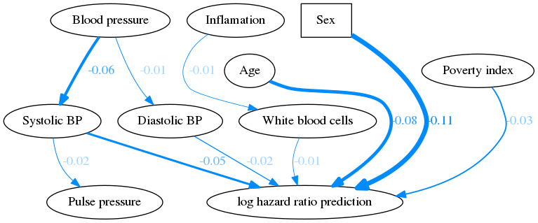
(a) Shapley Flow

Figure 17: Comparison among methods on 100 background samples from the nutrition dataset, showing top 10 features/edges.

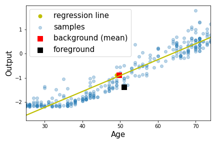
(a) Age vs. output

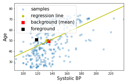
(b) Age vs. systolic blood pressure

Figure 18: Age appears to be highly risky in on-manifold SHAP because it steals credit from other variables.

11 Considering all histories could lead to boundary inconsistency

In this section, we give an example of how considering all history $\mathcal{H}$ in the axioms (as opposed to $\mathcal{\tilde{H}}$) could lead to inconsistent attributions across boundaries. Consider two cuts for the same causal graph shown in Figure 19. Note that both the green and the red cut share the edge “a”. We have $8$ possible message transmission histories (‘c’, ‘b’ can be transmitted only after ‘d’ has been transmitted): $\{[a,d,c,b],[a,d,b,c],[d,a,c,b],[d,a,b,c],[d,c,a,b],[d,c,b,a],[d,b,a,c],[d,b,c,a]\}$. We use the same notation for carrier games (defined in Section 8) and construct a game as the following:

$v_{red}=v_{red}^{dca}-v_{red}^{dcab}+v_{red}^{dba}-v_{red}^{dbac}$

Because of the linearity axiom, we have $\phi_{v_{red}}(a)>0,\phi_{v_{red}}(b)<0,\phi_{v_{red}}(c)<0,\phi_{v_{red}}(d)=0$.

However, when we consider the green boundary, the ordering $dcab$ and $dbac$ does not exist because in the green boundary $A$ and $Y$ are assumed to be a black-box. Therefore, $v_{green}=\boldsymbol{0}$, which means $a$ is now a dummy edge: $\phi_{v_{green}}(a)=0\neq\phi_{v_{red}}(a)$. This demonstrate that we cannot consider all histories in $\mathcal{H}$ and being boundary consistent.

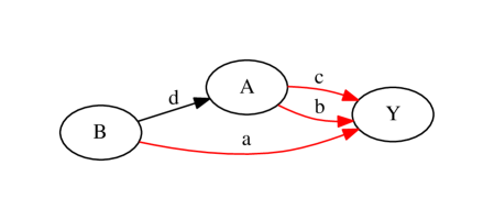
(a) Red cut

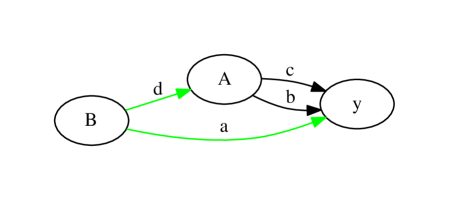
(b) Green cut

Figure 19: Two cuts that represent two boundaries for the same causal graph.

References

- Aas et al., (2019) Aas, K., Jullum, M., and Løland, A. (2019). Explaining individual predictions when features are dependent: More accurate approximations to shapley values. arXiv preprint arXiv:1903.10464.
- Adadi and Berrada, (2018) Adadi, A. and Berrada, M. (2018). Peeking inside the black-box: A survey on explainable artificial intelligence (xai). IEEE Access, 6:52138–52160.
- Baehrens et al., (2010) Baehrens, D., Schroeter, T., Harmeling, S., Kawanabe, M., Hansen, K., and Müller, K.-R. (2010). How to explain individual classification decisions. The Journal of Machine Learning Research, 11:1803–1831.
- Binder et al., (2016) Binder, A., Montavon, G., Lapuschkin, S., Müller, K.-R., and Samek, W. (2016). Layer-wise relevance propagation for neural networks with local renormalization layers. In International Conference on Artificial Neural Networks, pages 63–71. Springer.
- Breiman, (2001) Breiman, L. (2001). Random forests. Machine learning, 45(1):5–32.
- Chen et al., (2020) Chen, H., Janizek, J. D., Lundberg, S., and Lee, S.-I. (2020). True to the model or true to the data? arXiv preprint arXiv:2006.16234.
- Cox, (1998) Cox, C. S. (1998). Plan and operation of the NHANES I Epidemiologic Followup Study, 1992. Number 35. National Ctr for Health Statistics.
- Datta et al., (2016) Datta, A., Sen, S., and Zick, Y. (2016). Algorithmic transparency via quantitative input influence: Theory and experiments with learning systems. In 2016 IEEE symposium on security and privacy (SP), pages 598–617. IEEE.
- Dhamdhere et al., (2018) Dhamdhere, K., Sundararajan, M., and Yan, Q. (2018). How important is a neuron? arXiv preprint arXiv:1805.12233.
- Fisher et al., (2018) Fisher, A., Rudin, C., and Dominici, F. (2018). All models are wrong but many are useful: Variable importance for black-box, proprietary, or misspecified prediction models, using model class reliance. arXiv preprint arXiv:1801.01489, pages 237–246.
- Frye et al., (2020) Frye, C., de Mijolla, D., Cowton, L., Stanley, M., and Feige, I. (2020). Shapley-based explainability on the data manifold. arXiv preprint arXiv:2006.01272.
- Frye et al., (2019) Frye, C., Feige, I., and Rowat, C. (2019). Asymmetric shapley values: incorporating causal knowledge into model-agnostic explainability. arXiv preprint arXiv:1910.06358.
- Glymour et al., (2019) Glymour, C., Zhang, K., and Spirtes, P. (2019). Review of causal discovery methods based on graphical models. Frontiers in genetics, 10:524.
- Heskes et al., (2020) Heskes, T., Sijben, E., Bucur, I. G., and Claassen, T. (2020). Causal shapley values: Exploiting causal knowledge to explain individual predictions of complex models. Advances in neural information processing systems.
- Janzing et al., (2020) Janzing, D., Minorics, L., and Blöbaum, P. (2020). Feature relevance quantification in explainable ai: A causal problem. In International Conference on Artificial Intelligence and Statistics, pages 2907–2916. PMLR.
- López and Saboya, (2009) López, S. and Saboya, M. (2009). On the relationship between shapley and owen values. Central European Journal of Operations Research, 17(4):415.
- Lundberg et al., (2020) Lundberg, S. M., Erion, G., Chen, H., DeGrave, A., Prutkin, J. M., Nair, B., Katz, R., Himmelfarb, J., Bansal, N., and Lee, S.-I. (2020). From local explanations to global understanding with explainable ai for trees. Nature machine intelligence, 2(1):2522–5839.
- Lundberg et al., (2018) Lundberg, S. M., Erion, G. G., and Lee, S.-I. (2018). Consistent individualized feature attribution for tree ensembles. arXiv preprint arXiv:1802.03888.
- Lundberg and Lee, (2017) Lundberg, S. M. and Lee, S.-I. (2017). A unified approach to interpreting model predictions. In Advances in neural information processing systems, pages 4765–4774.
- Merrick and Taly, (2020) Merrick, L. and Taly, A. (2020). The explanation game: Explaining machine learning models using shapley values. In Holzinger, A., Kieseberg, P., Tjoa, A. M., and Weippl, E., editors, Machine Learning and Knowledge Extraction, pages 17–38, Cham. Springer International Publishing.
- Mittelstadt et al., (2019) Mittelstadt, B., Russell, C., and Wachter, S. (2019). Explaining explanations in ai. In Proceedings of the conference on fairness, accountability, and transparency, pages 279–288.
- Moraffah et al., (2020) Moraffah, R., Karami, M., Guo, R., Raglin, A., and Liu, H. (2020). Causal interpretability for machine learning-problems, methods and evaluation. ACM SIGKDD Explorations Newsletter, 22(1):18–33.
- Pearl, (2009) Pearl, J. (2009). Causality. Cambridge university press.
- Peters et al., (2017) Peters, J., Janzing, D., and Schölkopf, B. (2017). Elements of causal inference. The MIT Press.
- Robinson et al., (2020) Robinson, W. R., Renson, A., and Naimi, A. I. (2020). Teaching yourself about structural racism will improve your machine learning. Biostatistics, 21(2):339–344.
- Shapley, (1953) Shapley, L. S. (1953). A value for n-person games. Contributions to the Theory of Games, 2(28):307–317.
- Shrikumar et al., (2017) Shrikumar, A., Greenside, P., and Kundaje, A. (2017). Learning important features through propagating activation differences. arXiv preprint arXiv:1704.02685.
- Shrikumar et al., (2016) Shrikumar, A., Greenside, P., Shcherbina, A., and Kundaje, A. (2016). Not just a black box: Learning important features through propagating activation differences. arXiv preprint arXiv:1605.01713.
- Simonyan et al., (2013) Simonyan, K., Vedaldi, A., and Zisserman, A. (2013). Deep inside convolutional networks: Visualising image classification models and saliency maps. arXiv preprint arXiv:1312.6034.
- Springenberg et al., (2014) Springenberg, J. T., Dosovitskiy, A., Brox, T., and Riedmiller, M. (2014). Striving for simplicity: The all convolutional net. arXiv preprint arXiv:1412.6806.
- Štrumbelj and Kononenko, (2014) Štrumbelj, E. and Kononenko, I. (2014). Explaining prediction models and individual predictions with feature contributions. Knowledge and information systems, 41(3):647–665.
- Sundararajan and Najmi, (2019) Sundararajan, M. and Najmi, A. (2019). The many shapley values for model explanation. arXiv preprint arXiv:1908.08474.
- Sundararajan et al., (2017) Sundararajan, M., Taly, A., and Yan, Q. (2017). Axiomatic attribution for deep networks. International Conference on Machine Learning.
- Zhou et al., (2016) Zhou, B., Khosla, A., Lapedriza, A., Oliva, A., and Torralba, A. (2016). Learning deep features for discriminative localization. In Proceedings of the IEEE conference on computer vision and pattern recognition, pages 2921–2929.