Traffic Refinery: Cost-Aware Data Representation for Machine Learning on Network Traffic

Abstract.

Network management often relies on machine learning to make predictions about performance and security from network traffic. Often, the representation of the traffic is as important as the choice of the model. The features that the model relies on, and the representation of those features, ultimately determine model accuracy, as well as where and whether the model can be deployed in practice. Thus, the design and evaluation of these models ultimately requires understanding not only model accuracy but also the systems costs associated with deploying the model in an operational network. Towards this goal, this paper develops a new framework and system that enables a joint evaluation of both the conventional notions of machine learning performance (e.g., model accuracy) and the systems-level costs of different representations of network traffic. We highlight these two dimensions for two practical network management tasks, video streaming quality inference and malware detection, to demonstrate the importance of exploring different representations to find the appropriate operating point. We demonstrate the benefit of exploring a range of representations of network traffic and present Traffic Refinery, a proof-of-concept implementation that both monitors network traffic at 10 Gbps and transforms traffic in real time to produce a variety of feature representations for machine learning. Traffic Refinery both highlights this design space and makes it possible to explore different representations for learning, balancing systems costs related to feature extraction and model training against model accuracy.

1. Introduction

Network management tasks commonly rely on the ability to classify traffic by type or identify important events of interest from measured network traffic. Over the past 15 years, machine learning models have become increasingly integral to these tasks (Nguyen and Armitage, 2008; Singh and Nene, 2013; Boutaba et al., 2018). Training a machine learning model from network traffic typically involves extracting a set of features that achieve good model performance, a process that requires domain knowledge to know the features that are most relevant to prediction, as well as how to transform those features in ways that result in separation of classes in the underlying dataset. Figure 1 shows a typical pipeline, from measurement to modeling: The process begins with data (e.g., a raw traffic trace, summary statistics produced by a measurement system); features are then derived from this underlying data. The collection of features and derived statistics is often referred to as the data representation that is used as input to the model. Even for cases where the model itself learns the best representation based on its input (e.g., representation learning or deep learning), the designer of the algorithm must still determine the initial representation of the data that is provided to model.

Figure 1. Typical pipeline for model design in network inference.

Unfortunately, with existing network traffic measurement systems, the first three steps of this process—collection, cleaning, and feature engineering—are often out of the pipeline designer’s control. To date, most network management tasks that rely on machine learning from network traffic have assumed the data to be fixed or given, typically because decisions about measuring, sampling, aggregating, and storing network traffic data are made based on the capabilities (and constraints) of current standards and hardware capabilities (e.g., IPFIX/NetFlow). As a result, a model might be trained with a sampled packet trace or aggregate statistics about network traffic—not necessarily because that data representation would result in an efficient model with good overall performance, but rather because the decision about data collection was made well before any modeling or prediction problems were considered.

Existing network traffic measurement capabilities capture either flow-level statistics or perform fixed transformations on packet captures. First, flow-based monitoring collects coarse-grained statistics (e.g., IPFIX/NetFlow or collection infrastructure such as Kentik (kentik, 2019) and Deepfield (deepfield, 2019)). These statistics are also often based on samples of the underlying traffic (Estan and Varghese, 2002). Conversely, packet-level monitoring aims to capture traffic for specialized monitoring applications (corelight, 2019) or triggered on-demand to capture some subset of traffic for further analysis (Zhu et al., 2015). Programmable network hardware offers potential opportunities to explore how different data representations can improve model performance; yet, previous work on programmable hardware and network data structures has typically focused on efficient ways to aggregate statistics (Liu et al., 2016) (e.g., heavy hitter detection), rather than supporting different data representations for machine learning models. In all of these cases, decisions about data representation are made at the time of configuration or deployment, well before the analysis takes place. Once network traffic data is collected and aggregated, it is difficult, if not impossible, to retroactively explore a broader range of data representations that could potentially improve model performance.

A central premise of the work in this paper is introducing additional flexibility into the first three steps of this pipeline for network management tasks that rely on traffic measurements. On the surface, raw packet traces would seem to be an appealing starting point: Any network operator or researcher knows full well that raw packet traces offer maximum flexibility to explore transformations and representations that result in the best model performance. Yet, unfortunately, capturing raw packet traces often proves to be impractical on large networks as raw packet traces produce massive amounts of data, introducing storage and bandwidth requirements that are often prohibitive. Many controlled laboratory experiments (and much past work) that demonstrate a model’s accuracy turn out to be non-viable in practice because the systems costs of deploying and maintaining the model are prohibitive. An operator may ultimately need to explore costs across state, processing, storage, and latency to understand whether a given pipeline can work in its network.

Evaluation of a machine learning model for network management tasks must also consider the operational costs of deploying that model in practice. Such an evaluation requires exploring not only how data representation and models affect model accuracy, but also the systems costs associated with different representations. Sculley et al. refer to these considerations as “technical debt” (Sculley et al., 2015) and identified a number of hidden costs that contribute to building the technical debt of ML-systems, such as: unstable sources of data, underutilized data, use of generic packages, among others. This problem is vast and complex, and this paper does not explore all dimensions of this problem. For example, we do not investigate practical considerations such as model training time, model drift, the energy cost of training, model size, and many other practical considerations. In this regard, this paper scratches the surface of systemization costs, which we believe deserves more consideration before machine learning can be more widely deployed in operational networks.

To lay the groundwork for more research that considers these costs, we develop and publicly release a systematic approach to explore the relationship between different data representations for network traffic and (1) the resulting model performance as well as (2) their associated costs. We present Traffic Refinery (section 3), a proof-of-concept reference system implementation designed to explore network data representations and evaluate the systems-related costs of these representations. To facilitate exploration, Traffic Refinery implements a processing pipeline that performs passive traffic monitoring and in-network feature transformations at traffic rates of up to 10 Gbps in software (section 4). The pipeline supports capture and real-time transformation into a variety of common feature representations for network traffic; we have designed and exposed an API so that Traffic Refinery can be extended to define new representations, as well. In addition to facilitating the transformations thesemselves, Traffic Refinery performs profiling to quantify system costs, such as state and compute, for each transformation, to allow researchers and operators to evaluate not only the accuracy of a given model but the associated systems costs of the resulting representation.

We use Traffic Refinery to demonstrate the value of jointly exploring data representations for modeling and their associated costs for two supervised learning problems in networking: video quality inference from encrypted traffic and malware detection. We study two questions:

• How does the cost of feature representation vary with network speeds? We use Traffic Refinery to evaluate the cost of performing different transformations on traffic in real-time in deployed networks across three cost metrics: in-use memory (i.e., state), per packet processing (i.e., compute), and data volume generated (i.e., storage). We show that for the video quality inference models, state and storage requirements out-pace processing requirements as traffic rates increase (section 5.1.2). Conversely, processing and storage costs dominate the systems costs for the malware detection (section 5.2.2). These results suggest that fine-grained cost analysis can lead to different choices for traffic representation depending on different model performance requirements and network environments.

• Can systems costs be reduced without affecting model accuracy? We show that different data transformations allow systems designers to make meaningful decisions involving systems costs and model performance. For example, we find that state requirements can be significantly reduced for both problems without affecting model performance (section 5.1.3 and section 5.2.3), providing important opportunities for in-network reduction and aggregation.

While it is well-known that in general different data representations can both affect model accuracy and introduce variable systems costs, network research has left this area relatively under-explored. Our investigation both constitutes an important re-assessment of previous results and lays the groundwork for new directions in applying machine learning to network traffic modeling and prediction problems. From a scientific perspective, our work explores the robustness of previously published results. From a deployment standpoint, our results also speak to systems-level deployment considerations, and how those considerations might ultimately affect these models in practice, something that has been often overlooked in previous work. Looking ahead, we believe that incorporating these types of deployment costs as a primary model evaluation metric should act as a rubric for evaluating models that rely on machine learning for prediction and inference from network traffic.

2. Joint Exploration of Cost and Model Performance

Exploring the wide range of possible data representations can help improve model performance within the constraints of what is feasible with current network technologies. Doing so, however, requires a system that enables joint exploration of both systems cost and model performance. To this end, this section highlight two important requirements needed to support exploration: (1) the ability to flexibly define how features are extracted from traffic; and (2) integrated analysis of systems costs.

2.1. Flexible Feature Extraction

Different network inference tasks use different models, each of which may depend on a unique set of features. Consider the task of inferring the quality of a video streaming application from encrypted traffic (e.g., resolution). This problem is well-studied (Bronzino et al., 2019; Mazhar and Shafiq, 2018a; Mangla et al., 2019; Gutterman et al., 2019). The task has been commonly modeled using data representations extracted from different networking layers at regular intervals (e.g., every ten seconds). For instance, Bronzino et al. (Bronzino et al., 2019) grouped data representations from different networking layers into different feature sets: Network, Transport, and Application layer features. Network-layer features consist of lightweight information available from observing network flows (identified by the IP/port four-tuple) and are typically available in monitoring systems (e.g., NetFlow) (kentik, 2019; deepfield, 2019). Transport-layer features consist of information extracted from the TCP header, such as end-to-end latency and packet retransmissions. Such features are widely used across the networking space but can require significant resources (e.g., memory) to collect from large network links. Finally, application-layer metrics are those that include any feature related to the application data that can be gathered by solely observing packet patterns (i.e., without resorting to deep packet inspection). These features capture a unique behavior of the application and have been designed specifically for this problem.

We replicate the work of Bronzino et al. (Bronzino et al., 2019) by training multiple machine learning models to infer the resolution of video streaming applications over time using the three aforementioned data representations. Figure 2(a) shows the precision and recall achieved by each representation. We observe that the performance of a model trained with Network Layer features only (NetFlow in the figure) achieves the poorest performance, which agrees with previous results. Hence, relying solely on features offered by existing network infrastructure would have produced the worst performing models. On the other hand, combining Network and Application features results in more than a 10% increase in both precision and recall. This example showcases how limiting available data representations to the ones typically available from existing systems (e.g., NetFlow) can inhibit potential gains, highlighted by the blue-shaded area in Figure 2(a). This example highlights the need for extensible data collection routines that can evolve with Internet applications and the set of inference tasks.

(a) The relationship between data representations and model performance for video quality inference

(b) Storage cost for collecting a one hour of traffic across different monitoring system on a 10 Gbps link.

Figure 2. Balancing traffic data exploration and storage cost.

2.2. Integrated System Cost Analysis

Of course, any representation is possible if packet traces are the starting point, but raw packet capture can be prohibitive in operational networks, especially at high speeds. We demonstrate the amount of storage required to collect traces at scale by collecting a one-hour packet capture from a live 10 Gbps link. As shown in Figure 2(b), we observe that this generates almost 300 GB of raw data in an hour, multiple orders of magnitude more than aggregate representations such as IPFIX/NetFlow. Limiting the capture to solely storing packet headers reduces the amount of data generated, though not enough to make the approach practical. To compute a variety of statistics that would not be normally available from existing systems we would require an online system capable of avoiding the storage requirements imposed by raw packet captures.

Deploying an online system creates practical challenges caused by the volume and rate of traffic that must be analyzed. Failing to support adequate processing rates (i.e., experiencing packet drops) ultimately degrades the accuracy of the resulting features, potentially invalidating the models. Fortunately, packet capture at high rates in software has become increasingly feasible due to tools such as PF_RING (Deri et al., 2004) and DPDK (dpdk, 2018). Thus, in addition to exploiting the available technical capabilities to capture traffic at high rates, the system should implement techniques to maximize its ability to ingest traffic and lower the overhead of system processing. For example, the system has to efficiently limit heavyweight processing associated with certain features to subsets of traffic that are targeted by the inference problem being studied without resorting to sampling, which can negatively impact model performance.

Any feature transformation will introduce systems-related costs. A network monitoring system should make it possible to quantify the cost that such transformations impose. Thus, to explore the space of model performance and their associated systems costs, the system should provide an integrated mechanism to profile each feature.

Figure 3. Traffic Refinery system overview.

3. Exploring data representations with Traffic Refinery

To explore network traffic feature representations and its subsequent effect on both the performance of prediction models and collection cost, we need a way to easily collect different representations from network traffic. To enable such exploration, we implement Traffic Refinery, which works both for data representation design, helping network operators explore the accuracy-cost tradeoffs of different data representations for an inference task; and for customized data collection in production, whereby Traffic Refinery can be deployed online to extract custom features.

Data representation design has three steps. First, network operators or researchers define a superset of features worth exploring for the task and configure Traffic Refinery to collect all these features for a limited time period. Second, during this collection period, the system profiles the costs associated with collecting each individual feature. Finally, the resulting data enables the analysis of model accuracy versus traffic collection cost tradeoffs.

This section first describes the general packet processing pipeline of the system (Section 3.1) and how a user can configure this pipeline to collect features specific to a given inference task (Section 3.2). We then present how to profile the costs of features for data representation design (Section 3.3).

3.1. Packet Processing Pipeline

Figure 3 shows an overview of Traffic Refinery. Traffic Refinery is implemented in Go (golang, 2020) to exploit performance and flexibility, as well as its built-in benchmarking tools. The system design revolves around three guidelines: (1) Detect flows and applications of interest early in the processing pipeline to avoid unnecessary overhead; (2) Support state-of-the-art packet processing while minimizing the entry cost for extending which features to collect; (3) Aggregate flow statistics at regular time intervals and store for future consumption. The pipeline has three components:

1. a traffic categorization module responsible for associating network traffic with applications;

2. a packet capture and processing module that collects network flow statistics and tracks their state at line rate; moreover, this block implements a cache used to store flow state information; and

3. an aggregation and storage module that queries the flow cache to obtain features and statistics about each traffic flow and stores higher-level features concerning the applications of interest for later processing.

Traffic Refinery is customizable through a configuration file written in JSON. The configuration provides a way to tune system parameters (e.g., which interfaces to use for capture) as well as the definitions of service classes to monitor. A service class includes three pieces of information that establish a logical pipeline to collect the specified feature sets for each targeted service class: (1) which flows to monitor; (2) how to represent the underlying flows in terms of features; (3) at what time granularity features should be represented. Listing LABEL:lst:config shows the JSON format used.

⬇

1 {

2 "Name": "ServiceName",

3 "Filter": {

4 "DomainsString": ["domain.x", ...],

5 "Prefixes": ["10.0.0.0/18", ...]

6 },

7 "Collect": [FeatureSetA, FeatureSetB, ...],

8 "Emit": 10

9 }

Listing 1: Configuration example.

3.1.1. Traffic Categorization

Traffic Refinery aims to minimize overhead generated by the processing and state of packets and flows that are irrelevant for computing the features of interest. Accordingly, it is crucial to categorize network flows based on their service early so that the packet processing pipeline can extract features solely from relevant flows, ideally without resorting to sampling traffic. To accurately identify the sub-portions of traffic that require treatment online without breaking encryption or exporting private information to a remote server, Traffic Refinery implements a cache to map remote IP addresses to services accessed by users. The map supports identifying the services flows belong to by using one of two methods: (1) Using the domain name of the service: similarly to the approach presented by Plonka and Barford (Plonka and Barford, 2011), Traffic Refinery captures DNS queries and responses and inspects the hostname in DNS queries and matches these lookups against a corpus of regular expressions for domain names that we have derived for those corresponding services. For example, $\verb/(.+?\.)?nflxvideo\.net/$ captures domain names corresponding to Netflix’s video caches. (2) Using exact IP prefixes: For further flexibility, Traffic Refinery supports specifying matches between services and IP prefixes, which assists with mapping when DNS lookups are cached or encrypted.

Using DNS to map traffic to applications and services may prove challenging in the future, as DNS becomes increasingly transmitted over encrypted transport (e.g., DNS-over-HTTPS (Borgolte et al., 2019) or DNS-over TLS (Reddy et al., 2017)). In such situations, we envision Traffic Refinery relying on two possible solutions: (1) parse TLS handshakes for the server name indication (SNI) field in client hello messages, as this information is available in plaintext; or (2) implement a web crawler to automatically generate an IP-to-service mapping, a technique already implemented in production systems (deepfield, 2019).

3.1.2. Packet Capture and Processing

The traffic categorization and packet processing modules both require access to network traffic. To support fast (and increasing) network speeds, Traffic Refinery relies on state-of-the-art packet capture libraries: We implement Traffic Refinery’s first two modules and integrate a packet capture interface based on PF_RING (Deri et al., 2004) and the gopacket DecodingLayerParser library (gopacket, 2020). Traffic Refinery also supports libpcap-based packet capture and replay of recorded traces.

Processing network traffic in software is more achievable than it has been in the past; yet, supporting passive network performance measurement involves developing new efficient algorithms and processes for traffic collection and analysis. Traffic Refinery implements parallel traffic processing through a pool of worker processes, allowing the system to scale capacity and take advantage of multicore CPU architectures. We exploit flow clustering (in software or hardware depending on the available resources) to guarantee that packets belonging to the same flow are delivered to the same worker process, thus minimizing cross-core communication and ensuring thread safety. The workers store the computed state in a shared, partitioned flow cache, making it available for quick updates upon receiving new packets.

The packet processing module has two components:

State storage: Flow cache.

We implement a flow cache used to store a general data structure containing state and statistics related to a network flow. The general flow data structure allows storing different flow types, and differing underlying statistics using a single interface. Furthermore, it includes, if applicable, an identifier to match the services the flow belongs to. This information permits the system to determine early in the pipeline whether a given packet requires additional processing. The current version of the system implements the cache through a horizontally partitioned hash map. The cache purges entries for flows that have been idle for a configurable amount of time. In our configuration this timeout is set to 10 minutes.

Feature extraction: Service-driven packet processing.

A worker pool processes all non-DNS packets. Each worker has a dedicated capture interface to read incoming packets. As a first step, each worker pre-parses MAC, network, and transport headers, which yields useful information such as the direction of the traffic flow, the protocols, and the addresses and ports of the traffic. The system then performs additional operations on the packet depending on the service category assigned to the packet by inspecting the flow’s service identifier in the cache. Using the information specified by the configuration file, Traffic Refinery creates a list of feature classes to be collected for a given flow at runtime. Upon receiving a new packet and mapping it to its service, Traffic Refinery loops through the list and updates the required statistics.

3.1.3. Aggregation and Storage

Traffic Refinery exports high-level flow features and data representations at regular time intervals. Using the time representation information provided in the configuration file, Traffic Refinery initializes a timer-driven process that extracts the information of each service class at the given time intervals. Upon firing the collection event, the system loops through the flows belonging to a given service class and performs the required transformation (e.g., aggregation or sampling) to produce the data representation of the class. Traffic Refinery’s packet processing module exposes an API that provides access to the information stored in the cache. Queries can be constructed based on either an application (e.g., Netflix), or on a given device IP address. In the current version of the system, we implement the module to periodically query the API to dump all collected statistics for all traffic data representations to a temporary file in the system. We then use a separate system to periodically upload the collected information to a remote location, where it can be used as input to models.

3.2. User-Defined Traffic Representations

The early steps of any machine learning pipeline involve designing features that could result in good model performance. We design Traffic Refinery to facilitate the exploration of how different representations affect model performance and collection cost. To do so, we design Traffic Refinery to use convenient flow abstraction interfaces to allow for quick implementation of collection methods for features and their aggregated statistics. Each flow data structure implements two functions that define how to handle a packet in the latter two steps of the processing pipeline: (1) an AddPacket function that defines how to update the flow state metrics using the pre-processed information parsed from the packet headers; and (2) a CollectFeatures function that allows the user to specify how to aggregate the features collected for output when the collection time interval expires.

Implemented features are added as separate files. Traffic Refinery uses the configuration file to obtain the list of service class definitions and the features to collect for each one of them. Upon execution, the system uses Go’s language run-time reflection to load all available feature classes and select the required ones based on the system configuration. The implemented functions are then executed respectively during the packet processing step or during representation aggregation. We detail in Section 5 how the system can be configured to flexibly collect features at deployment time for two use cases: video quality inference and malware detection.

⬇

1 // PacketCounters is a data structure to collect packet and byte counters

2 type PacketCounters struct {

3 InCounter int64

4 OutCounter int64

5 InBytes int64

6 OutBytes int64

7 }

8

9 // AddPacket increment the counters based on information contained in pkt

10 func (c *PacketCounters) AddPacket(pkt *network.Packet) {

11 if pkt.Dir == network.TrafficIn {

12 c.InCounter++

13 c.InBytes += pkt.Length

14 } else if pkt.Dir == network.TrafficOut {

15 c.OutCounter++

16 c.OutBytes += pkt.Length

17 }

18 }

19

20 // PacketCountersOutput is a data structure that contains the features to output

21 type PacketCountersOutput struct {

22 KbpsUp float64

23 KbpsDw float64

24 PpsUp float64

25 PpsDw float64

26 }

27

28 // CollectFeatures calculates the features to output at given time intervals

29 func (c *PacketCounters) CollectFeatures(slotSize float64) PacketCountersOutput{

30 return PacketCountersOutput{

31 KbpsUp: float64(c.OutBytes) / (slotSize * 128.0)

32 KbpsDw: float64(c.InBytes) / (slotSize * 128.0)

33 PpsUp: float64(c.OutBytes) / slotSize

34 PpsDw: float64(c.InBytes) / slotSize

35 }

36 }

Listing 2: Implementing a new counters class.

As an example, we show in Listing LABEL:lst:counters our implementation of the PacketCounters feature class. This collection of features, stored in the PacketCounters data structure, keeps track of the number of packets and bytes for observed flows. To do so, the AddPacket function uses the pre-processed information which is stored in the Packet provided as input (i.e., the direction of the packet and its length). Upon triggering of the collection interval, the system uses the structure to output throughput and packets per-second statistics, i.e., the CollectFeatures function and the output data structure PacketCountersOutput. The current release of the system provides a number of built-in default features commonly collected across multiple layers of the network stack. Table 1 provides an overview of the features currently supported.

Group	Features
PacketCounters	throughput, packet counts
PacketTimes	packet interarrivals
TCPCounters	flag counters, window size, retransmissions, etc.
LatencyCounters	latency, jitter

Table 1. Current common features available in Traffic Refinery.

Design considerations.

We took this design approach to offer full flexibility in defining new features to collect while also minimizing the amount of knowledge required of a user about the inner mechanics of the system. We made several compromises in developing Traffic Refinery. First, our design focuses on supporting per-flow statistics and output them at regular time intervals. This approach enables the system to exploit established packet processing functions (e.g., clustering) to improve packet processing performance. Conversely, this solution might limit a user’s ability to implement specific types of features, such as features that require cross-flow information or those based on events. Second, the software approach for feature calculation proposed in Traffic Refinery might encourage a user to compute statistics that are ultimately unsustainable for an online system deployed in an operational network. To account for this possibility, the next section discusses how the system’s cost profiling method provides a way to quantify the cost impact that each feature imposes on the system. Ultimately, this analysis should provide feedback to a user in understanding whether such features should be considered for deployment.

3.3. Cost Profiling

Traffic Refinery aims to provide an intuitive platform to evaluate the system cost effects of the user defined data representations presented in the previous section. To do so, we use Go’s built-in benchmarking features and implement dedicated tools to profile different costs intrinsic to the collection process. At data representation design time, users employ the profiling method to quickly iterate through the collection of different features in isolation and provide a fair comparison for three cost metrics: state, processing, and storage.

State costs.

We aim to collect the amount of in-use memory over time for each feature class independently. To achieve this, we use Go’s pprof profiling tool. Using this tool, the system can output at a desired instant a snapshot of the entire in-use memory of the system. We extract from this snapshot the amount of memory that has been allocated by each service class at the end of each iteration of the collection cycle, i.e., the time the aggregation and storage module gathers the data from the cache, which corresponds to peak memory usage for each interval.

Processing costs.

To evaluate the CPU usage for each feature class, we aim to monitor the amount of time required to extract the feature information from each packet, leaving out any operation that shares costs across all possible classes, such as processing the packet headers or reading/writing into the cache. To do so, we build a dedicated time execution monitoring function that tracks the execution of each AddPacket function call in isolation, collecting running statistics (i.e., mean, median, minimum, and maximum) over time. This method is similar in spirit to Go’s built-in benchmarking feature but allows for using raw packets captured from the network for evaluation over longer periods of time.

Storage costs.

Storage costs can be compared by observing the size of the output generated over time during the collection process. The current version of the system stores this file in JSON format without implementing any optimization on the representation of the extracted information. While this solution can provide a general overview of the amount of data produced by the system, we expect that this feature will be further optimized for space in the future.

Cost profiling analysis.

Traffic Refinery supports two modes for profiling feature costs: (1) Profiling from live traffic: in this setting the system captures traffic from a network interface and collects statistics for a configurable time interval; and (2) Profiling using offline traffic traces: in this setting profiling runs over recorded traffic traces, which enables fine-grained inspection of specific traffic events (e.g., a single video streaming session) as well as repeatability and reproducibility of results. Similarly to Go’s built-in benchmarking tools, our profiling tools run as standalone executables. To select the sets of user-defined features (as described in Section 3.2) to profile, the profiling tool takes as input the same system configuration file used for executing the system. Upon execution, the system creates a dedicated measurement pipeline that collects statistics over time.

4. Prototype Evaluation

To examine the traffic processing capacity of Traffic Refinery, we deploy the system on a commodity server equipped with 16 Intel Xeon CPUs running at 2.4 GHz, and 64 GB of memory running Ubuntu 18.04. The server has a 10 GbE link that receives mirrored traffic from an interconnect link carrying traffic for a consortium of universities. The link routinely reaches nearly full capacity (e.g., roughly 9.8 Gbps) during peak times each day during the academic year. We evaluate Traffic Refinery on the link over several days in October 2020. We use the PF_RING packet library with zero-copy enabled in order to access packets with minimal overhead. We did not specifically engineer or optimize our prototype for high-speed processing in production environments—such optimization is not the focus of this paper—yet this setup nonetheless offers a realistic deployment representation in an ISP network where an operator might use Traffic Refinery to deploy its monitoring models, enables us to better understand potential system bottlenecks, and demonstrates that a production deployment of Traffic Refinery is feasible.

Figure 4(a) shows the number of packets processed and the number of packets dropped in 10-second windows over the course of a few days collecting the features required to infer video quality metrics in real time for eleven video services (more details on the use case are presented in the next section). Traffic tends to show a sharp increase mid-day, which coincides with an increase in the rate of packet drops. Overall, Traffic Refinery can process roughly one million packets per-second (10M PPS per ten-second window in the figure) without loss. Average packet size plays a significant role in the system’s capacity; for context, dShark (Yu et al., 2019) processes 3.3M PPS to process 40 Gbps by assuming average packet size of 1500 bytes. More specialized hardware, or faster general-purpose hardware could of course allow for for more parallel traffic processing workers and better performance.

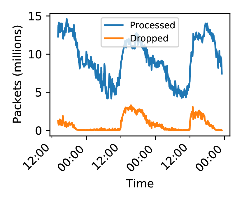
(a) Packets processed vs drops

(b) Flow cache size changes over time.

Figure 4. Traffic Refinery performance on the server.

We investigate the cause of packet drops to understand bottlenecks in Traffic Refinery. The system’s flow cache is a central component that is continuously updated concurrently by the workers that process traffic. We study the ability of the system’s flow cache to update the collected entries upon the receipt of new incoming packets. We implement benchmark tests that evaluate how many update operations the flow cache can perform each second in isolation from the rest of the system. We test two different scenarios: first, we evaluate the time to create a new entry in the cache, i.e., the operation performed upon the arrival of a newly seen flow. Second, we repeat the same process but for updates to existing flows in the cache. Our results show that new inserts take one order of magnitude more time than a simple update: roughly 6,000 nanoseconds (6 microseconds) versus 200 nanoseconds. Thus, the current flow cache implementation cannot support the creation of more than about 150,000 new flows per second.

We confirm this result by looking at the arrival of new flows in our deployment. Figure 4(b) shows the difference in the size of the flow cache between subsequent windows over the observation period. Negative values mean that the size of the flow cache decreased from one timestamp to the next. As shown, there are sudden spikes (e.g., greater than 100,000 new flows) in the number of flow entries in the cache around noon on two of the days, times that correspond with increases in packet drops. Recall that the flow cache maintains a data structure for every flow (identified by the IP/port four-tuple). The spikes are thus a result of Traffic Refinery processing a large number of previously unseen flows. This behavior helps explain the underlying causes for drops. Packets for flows that are not already in the flow cache cause multiple actions: First, Traffic Refinery searches the cache to check whether the flow already exists. Second, once it finds no entries, a new flow object is created and placed into the cache, which requires locks to insert an entry into the cache data structure. We believe that performance might be improved (i.e., drop rates could be lowered) by using a lock-free cache data structure and optimizing for sudden spikes in the number of new flows. Such optimizations are not the focus of this study, but we hope that our work lays the groundwork for follow-up work in this area.

5. Use Cases

In this section, we use Traffic Refinery to prototype two common inference tasks: streaming video quality inference and malware detection. For each problem, we conduct the three phases of the data representation design: (1) definition and implementation of a superset of candidate features; (2) feature collection and evaluation of system costs; and finally, (3) analysis of the cost-performance tradeoffs.

This exercise not only allows us to empirically measure systems-related costs of data representation for these problems, but also to demonstrate that the flexibility we advocate for developing network models is, in fact, achievable and required in practice. Our analysis shows that in both use cases we can significantly lower systems costs while preserving model performance. Yet, each use case presents different cost-performance tradeoffs: the dominant costs for video quality inference are state and storage, whereas for malware detection they are online processing and storage. Further, our analysis demonstrates that the ability to transform the data in different ways empowers systems designers to take meaningful decisions at deployment time that affect both systems costs as well as model performance.

5.1. Video Quality Inference Analysis

Video streaming quality inference often rely on features engineered by domain experts (Bronzino et al., 2019; Mazhar and Shafiq, 2018a; Mangla et al., 2019; Gutterman et al., 2019). We evaluate the models proposed by Bronzino et al. (Bronzino et al., 2019).

5.1.1. Traffic Refinery Customization

As discussed in Section 2, Bronzino et al. (Bronzino et al., 2019) categorized useful features for video quality inference into three groups that correspond to layers of the network stack: Network, Transport, and Application Layer features. In their approach, features are collected at periodic time intervals of ten seconds. The first ten seconds are used to infer the startup time of the video, while remaining time intervals are used to infer the ongoing resolution of the video being streamed.

We add approximately 100 lines of Go code to implement in Traffic Refinery the feature calculation functions to extract application features (i.e., VideoSegments). Further, we use built-in feature classes to collect network (i.e., PacketCounters) and transport (i.e., TCPCounters) features. We use these classes to configure the feature collection for 11 video services, including the four services studied in (Bronzino et al., 2019): Netflix, YouTube, Amazon Prime Video, and Twitch. We report a complete configuration used to collect Netflix traffic features in Appendix A. This use case, demonstrates how Traffic Refinery can be easily used to collect common features (e.g., flow counters collected in NetFlow) as well as extended to collect specific features useful for a given inference task.

5.1.2. Data Representation Costs

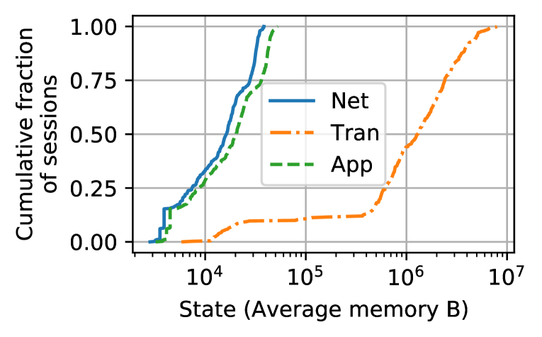
(a) State required for different features.

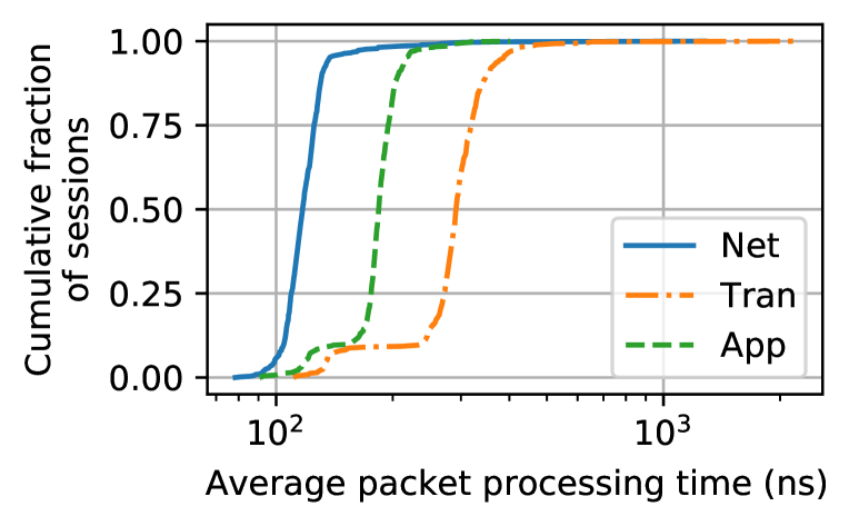
(b) Processing costs for different representations.

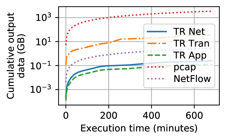
(c) Storage costs for different representations.

Figure 5. Cost profiling for video inference models.

We evaluate system-related costs of the three classes of features used for video quality inference problem: network, transport, and application features. First we use Traffic Refinery’s profiling tools to quantify the fine-grained costs imposed by tracking video streaming sessions. To do so, we profile the per-feature state and processing costs for pre-recorded packet traces with 1,000 video streaming sessions split across four major video streaming services (Netflix, YouTube, Amazon Prime Video, and Twitch). Then, we study the effect of collecting the different classes of features at scale by deploying the system in a 10 Gbps interconnect link.

We find that while some features add relatively little state (i.e., memory) and long-term storage costs, others require substantially more resources. Conversely, processing requirements are within the same order of magnitude for all three classes of features.

State Costs.

We study the state costs as the amount of in-use memory required by the system at the end of each collection cycle—i.e., the periodic interval at which the cache is dumped into the external storage. Figure 5(a) shows the cumulative distribution of memory in Bytes across all analyzed video streaming sessions. The reported results highlight how collecting transport layer features can heavily impact the amount of memory used by the system. In particular, collecting transport features can require up to three orders of magnitude more memory compared to network and application features. Transport features require historical flow information (e.g., all packets) in contrast with network features that require solely simple counters.

Further, the application features require a median of a few hundred MB in memory on the monitored link, with a slightly larger memory footprint than network features. At first glance, we assumed that this additional cost was due to the need for keeping in memory the information about video segments being streamed over the link. Upon inspection, however, we realized that streaming protocols request few segments at a time per time slot (across the majority of time slots the number of segments detected was lower than three), which leads to a minimal impact on memory used. We then concluded that this discrepancy was instead due to the basic Go data structure used to store video segments in memory, i.e., a slice, which requires extra memory to implement its functionality.

Processing Costs.

Collecting features on a running system measuring real traffic provides the ability to quantify the processing requirements for each target feature class. We represent the processing cost as the average processing time required to extract a feature set from a captured packet. Figure 5(b) shows distributions of the time required to process different feature classes. Collecting simple network counters requires the least processing time, followed by application and transport features.

While there are differences among the three classes, the difference is relatively small and within the same order of magnitude. These results highlight how all feature classes considered for video inference are relatively lightweight in terms of processing requirements. Hence, for this particular service class, state costs have a much larger impact than processing cost on the ability of collecting features in an operational network.

Storage Costs.

Feature retrieval at scale can generate high costs due to the need to move the collected data out of the measurement system and to the location where it will be ingested for processing. Figure 5(c) shows the amount of data produced by Traffic Refinery when collecting data for the three feature classes relevant to the video streaming quality inference on the monitored link. For comparison, we also include the same information for two different approaches to feature collection: (a) pcap, which collects an entire raw packet trace; (b) NetFlow configured using defaults (e.g., five minutes sampling), which collects aggregated per flow data volume statistics; this roughly corresponds to the same type of information collected by Traffic Refinery for the network layer features (i.e., TR Net in the figure).

Storage costs follow similar trends as the state costs previously shown. This is not surprising as the exported information is a representation of the state contained in memory. More interesting outcomes can be observed by comparing our system output to existing systems. Raw packet traces generate a possibly untenable amount of data and if used continuously can quickly generate terabytes of data. This result supports our claim that collecting traces at scale and for long periods of time quickly becomes impractical. Next, we notice that, even if not optimized, our current implementation produces less data than NetFlow, even when exporting similar information, i.e., network features. While this result mostly reflects the different verbosity levels of the configurations used for each system, it confirms that having additional flexibility in exporting additional features, e.g., video segments information, may introduce low additional cost. In the next section, we demonstrate that having such features available may result in significant model performance benefits.

5.1.3. Model Performance

In this section, we study the relationship between model performance and system costs for online video quality inference. We use previously developed models but explicitly explore how data representation affects model performance. We focus on state-related costs (i.e., memory), as for video quality inference, state costs mirror storage costs and the differences in processing costs of the feature classes is not significant (Section 5.1.2). Interestingly, we find that the relationship between state cost and model performance is not proportional. More importantly, we find that it is often possible to significantly reduce the state-related requirements of a model without significantly compromising prediction performance, further bolstering the case for systems like Traffic Refinery that allow for flexible data representations.

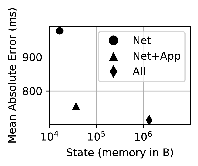
(a) Startup delay (lower is better).

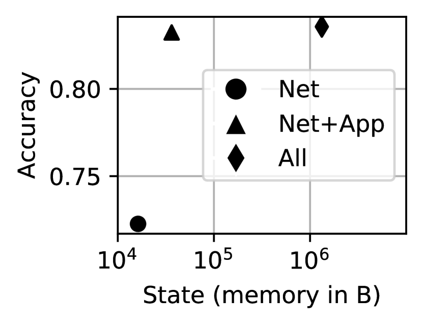
(b) Resolution (higher is better).

Figure 6. The relationship between features state cost and model performance for video streaming quality inference (marker shapes identify layers used and colors identify time interval size).

Representation vs. Model Performance.

To understand the relationship between memory overhead and inference accuracy, we use the dataset of more than 13k sessions presented in (Bronzino et al., 2019) to train six inference models for the two studied quality metrics: startup delay and resolution. For our analysis, we use the random forest models presented in (Bronzino et al., 2019); in particular, random forest regression for startup delay and random forest multi-class classifier for resolution. Further, we use the same inference interval size, i.e., ten-second time bins.

Figure 6 shows the relationship between model performance and state costs. As shown, network features alone can provide a lightweight solution to infer both startup delay and resolution but this yields the lowest model performance. Adding application layer features contributes to a very small additional memory overhead. This result is particularly important for resolution where models with video segments alone perform basically as well as combining all others. Further, adding transport features (labeled “All” in the figure) provides limited benefits in terms of added performance—40 ms on average lower errors for startup delay and less than 0.5% higher accuracy for resolution. Even for startup delay where using transport features can improve the mean absolute error by a larger margin, this comes at the cost of two orders of magnitude higher memory usage.

(a) Startup delay (lower is better).

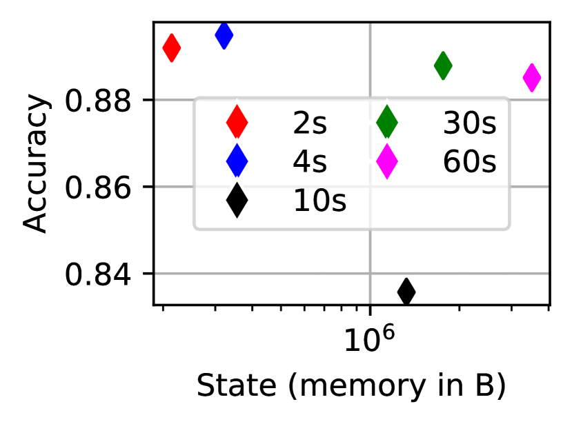
(b) Resolution (higher is better).

Figure 7. The relationship between time granularity state costs and model performance for video quality inference (marker shapes identify layers used and colors identify time interval size).

Time Granularity vs. Model Performance.

State of the art inference techniques (i.e., Bronzino et al. (Bronzino et al., 2019) and Mazhar and Shafiq (Mazhar and Shafiq, 2018b)) employ ten-second time bins to perform the prediction of the features. This decision is justified as a good tradeoff between the amount of information that can be gathered during each time slot, e.g., to guarantee that there is at least one video segment download in each bin, and the granularity at which the prediction is performed. For example, small time bins—e.g., two seconds— can have a very small memory requirement but might incur in lower prediction performance due to the lack of historical data on the ongoing session. On the other hand, larger time bins—e.g., 60 seconds—could benefit from the added information but would provide results that are just an average representation of the ongoing session quality. These behaviors can be particularly problematic for startup delay, a metric that would benefit from using exclusively the information of the time window during which the player is retrieving data before actually starting the video reproduction.

We train different random forest models with increasing time bin sizes of 2, 4, 10, 30, and 60 seconds. To understand the possible memory impact of the different time bins, we use all features (All) to train the models. In Figure 9, we observe different outcomes for the two quality metrics. For startup delay, the results show that ten-second windows can indeed provide a good tradeoff between memory and prediction accuracy, achieving a minimum of 70 ms better predictions than all other time granularities. This result shows that ten seconds is an acceptable tradeoff between gathering enough information at the beginning of a session without adding too much data from segment downloads that happens after the video has started.

Interestingly, the results for resolution inference show that ten-second windows perform the worst among all studied cases. This might be the product of multiple factors. In particular, the change of the inference window size not only changes how much information is used for prediction but it also affects the granularly of the inference, possibly modifying the underlying problem. Among the different time bin sizes we have different extremes ranging from two-second windows, which are about the length of the shortest video segments across all services, as well as 60-second time windows, which could contain many video quality changes within the time slot caused by the download of multiple video segments.

(a) State required for different features.

(b) Processing costs for different representations.

(c) Storage costs for different representations.

Figure 8. Cost profiling for the malware detection models.

(a) Image size (higher is better).

(b) Impact of method on costs.

Figure 9. The relationship between image size, processing method, and model performance for malware detection (marker shapes identify the method used and colors identify image size).

5.2. Malware Detection Analysis

In recent years, several works on traffic classification explored the application of deep learning on raw network traffic to solve a variety of inference tasks, such as malware detection (Marín et al., 2018; Wang et al., 2017b; Marín et al., 2020; Wang et al., 2017a) and service identification (Holland et al., 2020). Deep-learning based solutions differ from alternative approaches (e.g., the one used for the video inference in the previous section) in that they do not require to determine the initial representation of the data that is provided to the model but rather let the model learn the best representation based on its input. In practice, this means that applying such classifiers online requires to feed a Convolutionary Neural Network (CNN) with raw traffic data, represented either as a normalized sequence of bytes (Marín et al., 2018, 2020) or by converting the bytes into a gray-scale image (Wang et al., 2017b; Wang et al., 2017a).

The reduced complexity of these methods implies that the model and system designers’ role is limited to three choices: (1) the size of the input data collected from the traffic (e.g., for traffic flow classification, Wang et al. (Wang et al., 2017b) use the first 784 bytes of each flow, whereas DeepMAL (Marín et al., 2020) uses the first 100 bytes of payload of the first two packets of each flow); (2) the layers to collect such data from (e.g., packet headers and/or payload); and finally, (3) whether to perform data transformation (e.g., produce a PNG image from raw bytes) online or offline. In this section, we explore the impact of these different decisions on the deployment costs and model performance. We find that depending on the cost metrics under study there may not be a single “best” data representation, further bolstering the case for systems like Traffic Refinery that allow for flexible data representations exploration.

5.2.1. Traffic Refinery Customization

We add approximately 150 lines of Go code to implement both transformation methods in Traffic Refinery. For the first case, we implement a BytesCopyCounters data type that stores raw data extracted in a bytes array. Upon receiving new packets, the AddPacket function checks how much data is left to copy and, if any, it copies raw bytes from the correct layers into memory (i.e., headers, payload, or both). Once the bytes array is fully formed, no more packets are treated. Finally, the array is flushed into the output file when the collect function is invoked. For the second case, we implement a PNGCopyCounters data type that collects raw bytes from collected packets in a similar fashion but, also, converts the bytes into a PNG data structure when enough data has been collected. The data structure is flushed into the output file when the collect function is invoked.

5.2.2. Data Representation Costs

Similarly to the video inference use case, we use Traffic Refinery’s profiling tools to quantify the fine-grained costs imposed by the data collection required for deep neural network malware detection. For this task, we use the CIC-IDS2017 dataset (Sharafaldin et al., 2018), a standard dataset used for malware detection training and testing. The dataset consists of five days (working hours only) worth of pcap traces that contain a mix of lab-generated benign and malware traffic, for a total of ~171k flows distributed across the dataset. We divide the traces into ten minutes traffic sessions and profile the state, processing, and storage costs across different configurations.

We focus our presentation on two of the three design factors that affect possible configurations: (1) the data input size used to create the input image; and (2) whether to perform online data transformations. We do not present results on the impact of using different parts of the packets (i.e., headers, payload, or both) because our tests show that this configuration has relatively small impact on the cost profiles. For all presented results we solely use information collected from packet headers as recent work demonstrated that this is often sufficient for most inference tasks (Holland et al., 2020).

State Costs.

Figure 8(a) shows the cumulative distribution of memory in Bytes across all analyzed traffic sessions for different image sizes and techniques. As expected, the results follow the base intuition that state directly relates to the size of the memory allocated for each bytes array. Further, storing PNG images in memory causes state costs to roughly double, due to the need for allocating memory for both the raw bytes of memory as well as for the image.

Processing Costs.

Figure 8(b) shows distributions of the time required to process the input data for different configurations. Storing raw bytes in memory has a small impact on processing time, especially compared to the online creation of PNG images (a two orders of magnitude larger median). This behavior is expected since generating PNG images requires processing raw bytes through multiple filtering and compression stages (Duce, 2003).

Note that in this use case, most of the processing happens within the first few packets of each flow, which is the number of packets needed to achieve the desired input size for the CNN model. For this reason, flow size greatly impacts the average packet processing time where the majority of packets of a short flow are retained for processing, whereas the majority of packets of a large flow are not retained, and thus have negligible processing cost. To quantify this, we compute the average processing time for one session of the dataset while dividing encountered flows based on their size, i.e., in terms of the number packets that belong to the flow. For example, small flows (i.e., five packets or less) have an average processing time of 13,060 ns for the 28x28 PNG transformation case. In contrast, the average processing time for large flows (100 packets or more) is 335 ns. We observe similar results for all configurations.

Storage Costs.

Figure 8(c) shows the cumulative amount of data produced by Traffic Refinery when collecting data for different configurations over the entire dataset. Interestingly, while for small image sizes (e.g., 10x10) PNG encoding generates higher volumes of data, for larger ones (e.g., 28x28) it can save up to ~20% of total storage when compared to saving in raw bytes. This reduction happens thanks to the compression algorithms employed during the PNG encoding process. Compression is more effective when images contain solely packet headers, as multiple fields repeat across packets. This observation suggests that depending on the configuration employed in the system deployment, different strategies might be adopted regarding where to transform raw bytes into images.

5.2.3. Model Performance

To understand the relationship between costs and inference accuracy, we use the ~171k flows contained in the CIC-IDS2017 dataset (Sharafaldin et al., 2018) to train a CNN to classify traffic flows as either benign or malware. We follow the approach of Wang et al. (Wang et al., 2017b) by converting the sequence of bytes extracted into gray image PNGs before feeding them to the CNN; hence, we refer to the size of the sequence of bytes as the image size. We train 15 models in total using different configurations for image size (6x6, 10x10, 16x16, 20x20, and 28x28) and the layers of the network stack used to extract the sequence of bytes (header-fields only, payload only, or header-fields and payload). We observe that using payload only yields the lowest F1 score, while the other two configurations yield similar results (within a 3% F1 score difference). Given these small differences, we focus the remainder of this section on results varying configuration sizes alone. We perform the cost-performance analysis on a test set of 19k flows.

Representation vs. Model performance.

We explore the relationship between image size and inference performance. Figure 9(a) presents the F1 score obtained as we vary the image size. We present results solely for raw bytes, as F1 scores and cost trends are similar between the two methods. Image size has a clear impact on the model performance and the associated memory cost. The F1 score improves as the image size increases. However, this improvement flattens as the image size increases from a 20x20 to 28x28, whereas the induced cost in terms of memory cost maintained per-flow doubles. This result supports the need to explore the performance-cost relationship, as maintaining more information does not always lead to higher performance.

Following the results obtained in the previous section, we explore whether different configurations can lead to different tradeoffs and, consequently, different deployment strategies. Figure 9(b) shows the storage costs in terms of average storage per flow generated against the average processing time for different configurations. While processing times are consistently orders of magnitude higher when the PNG generation is integrated within the processing pipeline, storage costs have the opposite trend for larger image configurations, which are also the best performing ones. This result suggests that while converting an image can be computationally unfeasible under certain deployment settings, it might be preferable to perform it online for scenarios where storage is a major constraint.

6. Related Work

Machine learning models have become integral for solving many network management tasks (Nguyen and Armitage, 2008; Singh and Nene, 2013; Boutaba et al., 2018), from performance inference to security. Collecting input data to build models for network management tasks can be typically achieved with passive network monitoring tools, such as packet captures (e.g., libpcap (tcpdump, 2020) and its derivative applications Wireshark (Orebaugh et al., 2006) and Tshark (tshark, 2020)) or flow captures (e.g., NetFlow (Claise, 2004), IPFIX (Claise et al., 2013)). Unfortunately, this set of network monitoring tools inhibits model designers from exploring the space of possible data representations. On one hand, packet captures generate massive volume of data which makes them a none-viable approach for large networks. On the other, flow captures produce statistical information that are too coarse grained to enable full exploration of all possible data representations. Similarly, streaming analytics platforms (Cranor et al., 2003; Borders et al., 2012; Yuan et al., 2017; Narayana et al., 2017; Gupta et al., 2018) and algorithms (e.g., “sketches”) (Yu et al., 2013; Kumar et al., 2004; Liu et al., 2016; Yang et al., 2018) allow operators to express queries on streaming traffic data but they are primarily designed to collect low-level statistics on a backbone router or switch, or a programmable datacenter switch, which operate at very high speeds. As such, they typically support a more limited set of queries that are constrained by the hardware they are designed to support.

To obviate to the limitations of packet capture tools at scale, dShark (Yu et al., 2019) implements a distributed computing engine for processing distributed network traces, at scale, in the data center. As in Traffic Refinery, dShark offers a programming interface that permits (1) declaring groups of packet summaries that have similar properties and (2) defining queries that operate on such packets. Traffic Refinery differs in its design as it focuses on transformations as input to machine learning models. Conversely, dShark focuses its design on multi-point collection and transformations required for general diagnosis. Further, Traffic Refinery focuses on helping model designers evaluate both model accuracy and systems-related costs associated with data collection.

Advanced network monitoring and analysis tools such as Tstat (Mellia et al., 2003; Finamore et al., 2010), Bro (Paxson, 1999), and Snort (Roesch et al., 1999) are closest in spirit to Traffic Refinery in that they have the goal of capturing network traffic and executing transformations on the data for later use. Tstat is an open source passive monitoring tool that can monitor network traffic and output logs, statistics, and histograms with different granularities: per-packet, per-flow, or aggregated. Bro and Snort are network intrusion detection systems that rely on regular expressions to identify the subset of packets to inspect and execute specific tasks based on the class of traffic. Ultimately, these tools would need to be adapted to achieve custom feature representation, data representation exploration, and profiling data collection costs. Some commercial products apply machine learning to network traffic (e.g., Nokia’s Traffica (traffica, 2020), Deepfield (deepfield, 2019), NIKSUN’s NetCVR (netvcr, 2020)); these approaches are are proprietary and address a specific problem (e.g., customer support). On the other hand, Traffic Refinery is open-source, and permits jointly evaluating model performance and features collection costs at design time.

Recent work has also considered the costs associated with ML-systems (Sculley et al., 2015; Breck et al., 2017; Bronzino et al., 2019). Bronzino et al. addressed the problem of inferring the quality of video streaming applications from encrypted traffic and classified the possible set of features based on their corresponding layer in the network stack. This categorization enabled the authors to logically reason about the cost associated with each features sets. The observations about the tradeoffs between model accuracy and systems costs for a specific problem motivated us to explore this problem in general. Sculley et al., (Sculley et al., 2015) and Breck et al. (Breck et al., 2017) investigated the hidden “technical debt” that incurs during the development and deployment of ML systems; the authors discuss system-level factors that increase the maintenance costs of real-world ML systems over time (e.g., unstable or underutilized data, dependencies on proprietary packages, entanglement of input signals, to name a few). Traffic Refinery builds on this work, developing techniques to explore and mitigate technical debt associated with data representation.

7. Conclusion

This paper introduces Traffic Refinery, which permits consideration of both model accuracy and the systems-related costs of machine learning models trained on network traffic representations to make predictions concerning performance and security. We show the need for exploring more flexible representations first by showing that today’s default representations result in lower model accuracy. We present the design and implementation of Traffic Refinery and apply it to two use case studies: video quality performance inference and malware detection. This work has demonstrated both the need and the potential for exploring how different data representations can affect model accuracy, laying the groundwork for future work along multiple avenues, including automated exploration of data representations, systems-level optimizations to improve traffic processing capabilities and rates, and follow-up work that considers the design of processing hardware in concert with the need for specific data representations that result in high model accuracy across a range of inference problems. To enable the community to explore these benefits on a wider range of problems, we have both released Traffic Refinery as open-source software, as well as the evaluation in this paper.

Appendix A Video Quality Inference Configuration Details

This section provides additional details regarding the configuration and implementation in Traffic Refinery of the video quality inference use case.

A.1. Configuration

Listing LABEL:lst:netflix_config shows a complete configuration used to collect Netflix traffic features. The configuration includes filters for known Netflix domains, as well Netflix owned IP network prefixes. Further, the configuration instructs Traffic Refinery to collect the features for the three different classes described in Section 5, i.e., PacketCounters, TCPCounters, and VideoSegments. Finally, the statistics produced from these features are collected at ten seconds intervals.

⬇

1 {

2 "Name": "Netflix",

3 "Filter": {

4 "DomainsString": ["netflix.com","nflxvideo.net","nflximg.net","nflxext.com","nflximg.com","nflxso.net"],

5 "Prefixes": "23.246.0.0/18", "37.77.184.0/21", "45.57.0.0/17", "64.120.128.0/17", "66.197.128.0/17", "108.175.32.0/20", "185.2.220.0/22", "185.9.188.0/22", "192.173.64.0/18", "198.38.96.0/19", "198.45.48.0/20", "208.75.79.0/24", "2620:10c:7000::/44", "2a00:86c0::/32"]

6 },

7 "Collect": [PacketCounters, TCPCounters, VideoSegments],

8 "Emit": 10

9 }

Listing 3: Configuration to capture video features for Netflix.

A.2. Implementation

Listing LABEL:lst:video_counters shows the AddPacket implementation used to collect video segments information for the video quality inference use case. The function implements the technique first presented by Vengatanathan et al. (Krishnamoorthi et al., 2017) who showed how video segment information can be extracted by observing patterns in upstream traffic. In particular, this method uses upstream requests times to break down the stream of downstream packets into video segments.

⬇

1 // VideoSegment is used to keep track of segments in

2 // download

3 type VideoSegment struct {

4 Len int64

5 Seq int64

6 TsStart int64

7 TsEnd int64

8 LastPkt int64

9 DownPkts int64

10 DonwBytes int64

11 MaxDSeq int64

12 }

13

14 // VideoSegments is the flow stats structure used

15 // to store segments information

16 type VideoSegments struct {

17 CompleteSegments []VideoSegment

18 RunningSegment VideoSegment

19 }

20

21 const (

22 // QUICHeaderLen represents the minimum length in

23 // bytes to determine when a QUIC upstream packet

24 // contains payload

25 QUICHeaderLen = 100

26 )

27

28 // AddPacket updates the flow states based on the

29 // packet pkt

30 func (vf *VideoSegments) AddPacket(pkt *network.Packet) error {

31 if pkt.Dir == network.TrafficOut {

32 if (pkt.IsTCP && pkt.DataLength > 0) || (!pkt.IsTCP && pkt.DataLength > QUICHeaderLen) {

33 if vf.RunningSegment.TsStart != 0 && vf.RunningSegment.DownPkts > 0 {

34 vf.RunningSegment.TsEnd = vf.RunningSegment.LastPkt

35 vf.CompleteSegments = append(vf.CompleteSegments, vf.RunningSegment)

36 }

37 vf.RunningSegment = VideoSegment{Len: int64(pkt.Length), TsStart: pkt.TStamp, Seq: int64(pkt.Tcp.Seq)}

38 }

39 } else if pkt.DataLength > 0 {

40 vf.RunningSegment.DownPkts++

41 vf.RunningSegment.DonwBytes += int64(pkt.DataLength)

42

43 if int64(pkt.Tcp.Seq) > vf.RunningSegment.MaxDSeq {

44 vf.RunningSegment.MaxDSeq = int64(pkt.Tcp.Seq)

45 }

46 if pkt.TStamp > vf.RunningSegment.TsEnd {

47 vf.RunningSegment.LastPkt = pkt.TStamp

48 }

49 }

50 return nil

51 }

Listing 4: Implementing the VideoSegments counters

References

- (1)
- Borders et al. (2012) Kevin Borders, Jonathan Springer, and Matthew Burnside. 2012. Chimera: A Declarative Language for Streaming Network Traffic Analysis. In Presented as part of the 21st USENIX Security Symposium (USENIX Security 12). USENIX, Bellevue, WA, 365–379. https://www.usenix.org/conference/usenixsecurity12/technical-sessions/presentation/borders
- Borgolte et al. (2019) Kevin Borgolte, Tithi Chattopadhyay, Nick Feamster, Mihir Kshirsagar, Jordan Holland, Austin Hounsel, and Paul Schmitt. 2019. How DNS over HTTPS is Reshaping Privacy, Performance, and Policy in the Internet Ecosystem. Performance, and Policy in the Internet Ecosystem (July 27, 2019) (2019).
- Boutaba et al. (2018) Raouf Boutaba, Mohammad A Salahuddin, Noura Limam, Sara Ayoubi, Nashid Shahriar, Felipe Estrada-Solano, and Oscar M Caicedo. 2018. A comprehensive survey on machine learning for networking: evolution, applications and research opportunities. Journal of Internet Services and Applications 9, 1 (2018), 16.
- Breck et al. (2017) Eric Breck, Shanqing Cai, Eric Nielsen, Michael Salib, and D Sculley. 2017. The ml test score: A rubric for ml production readiness and technical debt reduction. In 2017 IEEE International Conference on Big Data (Big Data). IEEE, 1123–1132.
- Bronzino et al. (2019) Francesco Bronzino, Paul Schmitt, Sara Ayoubi, Guilherme Martins, Renata Teixeira, and Nick Feamster. 2019. Inferring Streaming Video Quality from Encrypted Traffic: Practical Models and Deployment Experience. Proceedings of the ACM on Measurement and Analysis of Computing Systems 3, 3 (2019), 1–25.
- Claise (2004) Benoit Claise. 2004. Cisco systems netflow services export version 9. Technical Report.
- Claise et al. (2013) Benoit Claise, Brian Trammell, and Paul Aitken. 2013. Specification of the IP flow information export (IPFIX) protocol for the exchange of flow information. (2013). RFC 7011.
- corelight (2019) corelight 2019. Corelight. https://corelight.com/. (2019).
- Cranor et al. (2003) Chuck Cranor, Theodore Johnson, Oliver Spataschek, and Vladislav Shkapenyuk. 2003. Gigascope: a stream database for network applications. In Proceedings of the 2003 ACM SIGMOD international conference on Management of data. ACM, 647–651.
- deepfield (2019) deepfield 2019. Deepfield. https://deepfield.com/. (2019).
- Deri et al. (2004) Luca Deri et al. 2004. Improving passive packet capture: Beyond device polling. In Proceedings of SANE, Vol. 2004. Amsterdam, Netherlands, 85–93.
- dpdk (2018) dpdk 2018. DPDK, Data Plane Development Kit. https://www.dpdk.org/. (2018).
- Duce (2003) David Duce. 2003. Portable Network Graphics (PNG) Specification (Second Edition). (2003). W3C Recommendation.
- Estan and Varghese (2002) Cristian Estan and George Varghese. 2002. New Directions in Traffic Measurement and Accounting. In Proceedings of the 2002 Conference on Applications, Technologies, Architectures, and Protocols for Computer Communications (SIGCOMM ’02). ACM, New York, NY, USA, 323–336. https://doi.org/10.1145/633025.633056
- Finamore et al. (2010) Alessandro Finamore, Marco Mellia, Michela Meo, Maurizio M Munafò, and Dario Rossi. 2010. Live traffic monitoring with tstat: Capabilities and experiences. In International Conference on Wired/Wireless Internet Communications. Springer, 290–301.
- golang (2020) golang 2020. Go language. https://golang.org/. (2020).
- gopacket (2020) gopacket 2020. Go Packet Library. (2020). https://godoc.org/github.com/google/gopacket.
- Gupta et al. (2018) Arpit Gupta, Rob Harrison, Marco Canini, Nick Feamster, Jennifer Rexford, and Walter Willinger. 2018. Sonata: Query-driven Streaming Network Telemetry. In Proceedings of the 2018 Conference of the ACM Special Interest Group on Data Communication (SIGCOMM ’18). ACM, New York, NY, USA, 357–371. https://doi.org/10.1145/3230543.3230555
- Gutterman et al. (2019) Craig Gutterman, Katherine Guo, Sarthak Arora, Xiaoyang Wang, Les Wu, Ethan Katz-Bassett, and Gil Zussman. 2019. Requet: Real-time qoe detection for encrypted youtube traffic. In Proceedings of the 10th ACM Multimedia Systems Conference. 48–59.
- Holland et al. (2020) Jordan Holland, Paul Schmitt, Nick Feamster, and Prateek Mittal. 2020. nPrint: A Standard Data Representation for Network Traffic Analysis. (2020). arXiv:2008.02695 https://arxiv.org/abs/2008.02695
- kentik (2019) kentik 2019. Kentik. https://kentik.com/. (2019).
- Krishnamoorthi et al. (2017) Vengatanathan Krishnamoorthi, Niklas Carlsson, Emir Halepovic, and Eric Petajan. 2017. BUFFEST: Predicting Buffer Conditions and Real-time Requirements of HTTP (S) Adaptive Streaming Clients. In Proceedings of the 8th ACM on Multimedia Systems Conference. ACM, 76–87.
- Kumar et al. (2004) Abhishek Kumar, Minho Sung, Jun Jim Xu, and Jia Wang. 2004. Data streaming algorithms for efficient and accurate estimation of flow size distribution. In ACM SIGMETRICS Performance Evaluation Review, Vol. 32. ACM, 177–188.
- Liu et al. (2016) Zaoxing Liu, Antonis Manousis, Gregory Vorsanger, Vyas Sekar, and Vladimir Braverman. 2016. One sketch to rule them all: Rethinking network flow monitoring with univmon. In Proceedings of the 2016 ACM SIGCOMM Conference. ACM, 101–114.
- Mangla et al. (2019) Tarun Mangla, Emir Halepovic, Mostafa Ammar, and Ellen Zegura. 2019. Using session modeling to estimate HTTP-based video QoE metrics from encrypted network traffic. IEEE Transactions on Network and Service Management 16, 3 (2019), 1086–1099.
- Marín et al. (2018) Gonzalo Marín, Pedro Casas, and Germán Capdehourat. 2018. Rawpower: Deep learning based anomaly detection from raw network traffic measurements. In Proceedings of the ACM SIGCOMM 2018 Conference on Posters and Demos. 75–77.
- Marín et al. (2020) Gonzalo Marín, Pedro Casas, and Germán Capdehourat. 2020. DeepMAL–Deep Learning Models for Malware Traffic Detection and Classification. arXiv preprint arXiv:2003.04079 (2020).
- Mazhar and Shafiq (2018a) M Hammad Mazhar and Zubair Shafiq. 2018a. Real-time video quality of experience monitoring for https and quic. In IEEE INFOCOM 2018-IEEE Conference on Computer Communications. IEEE, 1331–1339.
- Mazhar and Shafiq (2018b) M. Hammad Mazhar and Zubair Shafiq. 2018b. Real-time Video Quality of Experience Monitoring for HTTPS and QUIC. In INFOCOM, 2018 Proceedings IEEE. IEEE.
- Mellia et al. (2003) Marco Mellia, Andrea Carpani, and Renato Lo Cigno. 2003. Tstat: TCP statistic and analysis tool. In International Workshop on Quality of Service in Multiservice IP Networks. Springer, 145–157.
- Narayana et al. (2017) Srinivas Narayana, Anirudh Sivaraman, Vikram Nathan, Prateesh Goyal, Venkat Arun, Mohammad Alizadeh, Vimalkumar Jeyakumar, and Changhoon Kim. 2017. Language-directed hardware design for network performance monitoring. In Proceedings of the Conference of the ACM Special Interest Group on Data Communication. ACM, 85–98.
- netvcr (2020) netvcr 2020. NIKSUN NetVCR. https://www.niksun.com/product.php?id=110. (2020).
- Nguyen and Armitage (2008) Thuy TT Nguyen and Grenville Armitage. 2008. A survey of techniques for internet traffic classification using machine learning. IEEE communications surveys & tutorials 10, 4 (2008), 56–76.
- Orebaugh et al. (2006) Angela Orebaugh, Gilbert Ramirez, and Jay Beale. 2006. Wireshark & Ethereal network protocol analyzer toolkit. Elsevier.
- Paxson (1999) Vern Paxson. 1999. Bro: a system for detecting network intruders in real-time. Computer networks 31, 23-24 (1999), 2435–2463.
- Plonka and Barford (2011) David Plonka and Paul Barford. 2011. Flexible traffic and host profiling via DNS rendezvous. In Workshop Satin.
- Reddy et al. (2017) Tirumaleswar Reddy, Dan Wing, and Prashanth Patil. 2017. Dns over datagram transport layer security (dtls). RFC 8094 (2017).
- Roesch et al. (1999) Martin Roesch et al. 1999. Snort: Lightweight intrusion detection for networks.. In Lisa, Vol. 99. 229–238.
- Sculley et al. (2015) David Sculley, Gary Holt, Daniel Golovin, Eugene Davydov, Todd Phillips, Dietmar Ebner, Vinay Chaudhary, Michael Young, Jean-Francois Crespo, and Dan Dennison. 2015. Hidden technical debt in machine learning systems. In Advances in neural information processing systems. 2503–2511.
- Sharafaldin et al. (2018) Iman Sharafaldin, Arash Habibi Lashkari, and Ali A Ghorbani. 2018. Toward generating a new intrusion detection dataset and intrusion traffic characterization.. In ICISSP. 108–116.
- Singh and Nene (2013) Jayveer Singh and Manisha J Nene. 2013. A survey on machine learning techniques for intrusion detection systems. International Journal of Advanced Research in Computer and Communication Engineering 2, 11 (2013), 4349–4355.
- tcpdump (2020) tcpdump 2020. tcpdump and libpcap. https://www.tcpdump.org/. (2020).
- traffica (2020) traffica 2020. Nokia Traffica. https://www.nokia.com/networks/products/traffica/. (2020).
- tshark (2020) tshark 2020. Tshark: terminal-based Wireshark. https://www.wireshark.org/docs/wsug_html_chunked/AppToolstshark.html. (2020).
- Wang et al. (2017a) Wei Wang, Yiqiang Sheng, Jinlin Wang, Xuewen Zeng, Xiaozhou Ye, Yongzhong Huang, and Ming Zhu. 2017a. HAST-IDS: Learning hierarchical spatial-temporal features using deep neural networks to improve intrusion detection. IEEE Access 6 (2017), 1792–1806.
- Wang et al. (2017b) Wei Wang, Ming Zhu, Xuewen Zeng, Xiaozhou Ye, and Yiqiang Sheng. 2017b. Malware traffic classification using convolutional neural network for representation learning. In 2017 International Conference on Information Networking (ICOIN). IEEE, 712–717.
- Yang et al. (2018) Tong Yang, Jie Jiang, Peng Liu, Qun Huang, Junzhi Gong, Yang Zhou, Rui Miao, Xiaoming Li, and Steve Uhlig. 2018. Elastic sketch: Adaptive and fast network-wide measurements. In Proceedings of the 2018 Conference of the ACM Special Interest Group on Data Communication. ACM, 561–575.
- Yu et al. (2019) Da Yu, Yibo Zhu, Behnaz Arzani, Rodrigo Fonseca, Tianrong Zhang, Karl Deng, and Lihua Yuan. 2019. dShark: A general, easy to program and scalable framework for analyzing in-network packet traces. In 16th USENIX Symposium on Networked Systems Design and Implementation (NSDI 19). 207–220.
- Yu et al. (2013) Minlan Yu, Lavanya Jose, and Rui Miao. 2013. Software Defined Traffic Measurement with OpenSketch. In Presented as part of the 10th USENIX Symposium on Networked Systems Design and Implementation (NSDI 13). 29–42.
- Yuan et al. (2017) Yifei Yuan, Dong Lin, Ankit Mishra, Sajal Marwaha, Rajeev Alur, and Boon Thau Loo. 2017. Quantitative Network Monitoring with NetQRE. In Proceedings of the Conference of the ACM Special Interest Group on Data Communication (SIGCOMM ’17). ACM, New York, NY, USA, 99–112. https://doi.org/10.1145/3098822.3098830
- Zhu et al. (2015) Yibo Zhu, Nanxi Kang, Jiaxin Cao, Albert Greenberg, Guohan Lu, Ratul Mahajan, Dave Maltz, Lihua Yuan, Ming Zhang, Ben Y Zhao, et al. 2015. Packet-level telemetry in large datacenter networks. In ACM SIGCOMM Computer Communication Review, Vol. 45. ACM, 479–491.