Collisionless sound of bosonic superfluids in lower dimensions

Abstract

The superfluidity of low-temperature bosons is well established in the collisional regime. In the collisionless regime, however, the presence of superfluidity is not yet fully clarified, in particular in lower spatial dimensions. Here we compare the Vlasov-Landau equation, which does not take into account the superfluid nature of the bosonic system, with the Andreev-Khalatnikov equations, which instead explicitly contain a superfluid velocity. We show that recent experimental data of the sound mode in a two-dimensional collisionless Bose gas of ⁸⁷Rb atoms are in good agreement with both theories but the sound damping is better reproduced by the Andreev-Khalatnikov equations below the Berezinskii-Kosterlitz-Thouless critical temperature $T_{c}$ while above $T_{c}$ the Vlasov-Landau results are closer to the experimental ones. For one dimensional bosonic fluids, where experimental data are not yet available, we find larger differences between the sound velocities predicted by the two transport theories and, also in this case, the existence of a superfluid velocity reduces the sound damping.

I Introduction

According to Landau landau1941 , the liquid helium below the critical temperature is characterized by a superfluid component and a normal component. This idea was inspired by similar models used for superconductors london1935 and superfluids tisza1938 . In the standard hydrodynamic treatment of a neutral superfluid ll6 ; khalatnikov1965 ; schmitt2014 the normal component is supposed to be in the collisional regime. The very special case of the collisionless superfluid Helium-4, where the normal component is in the collisionless regime was analyzed by Andreev and Khalatnikov andreev1963 . In the collisionless regime khalatnikov1965 ; ll10 the dimensionless parameter $\omega\tau_{c}$ is such that $\omega\tau_{c}\gg 1$, where $\tau_{c}$ is the collision time of quasi-particles ll10 and $\omega$ is the frequency of a generic macroscopic oscillation travelling along the fluid. Usually $\tau_{c}$ grows by decreasing the temperature $T$, and at extremely low temperature one expects that collisionless phenomena dominate the dynamics of superfluids and, more generally, the dynamics of quantum liquids. Indeed, the Andreev and Khalatnikov andreev1963 collisionless approach is in full agreement with experimental measurements whitney of the sound velocity of Helium-4 for the temperature below $0.4$ Kelvin. In general, depending on size and density, the system can be in the collisionless regime also far from zero temperature ll6 ; khalatnikov1965 ; schmitt2014 ; andreev1963 ; ll10 . Actually, natural systems as ionized plasmas do exist which, due to the velocity dependence of the collision frequency, become collisionless in the opposite regime of very high temperature nicholson .

The interest in collisionless superfluids has been renewed by a recent experiment ville2018 , where the sound mode was measured in a uniform quasi-2D Bose gas made of ⁸⁷Rb atoms. The experimental data of the speed of sound are in good agreement with theoretical results ota2018 ; cappellaro2018 based on the Vlasov-Landau equation vlasov1945 ; landau46 (which is substantially equivalent to the random-phase approximation lipparini ) for neutral collisionless bosons. There are, however, some discrepancies between the experimental data of sound damping and the prediction of the Vlasov-Landau equation ota2018 . Very recently it has been shown china that the second sound of modified two-fluid hydrodynamic equations, which incorporate the dynamics of the quantized vortices, reproduce quite well the experimental sound velocity of Ref. ville2018 . However, in this dynamical Kosterlitz-Thouless theory china there is a fitting parameter in the dielectric function which makes this theory not really predictive. In Refs. ota2018 ; cappellaro2018 the superfluid nature of the system is not taken into account: the superfluid velocity ${\bf v}_{s}({\bf r},t)$ does not appear and the phase-space distribution $f({\bf r},{\bf p},t)$ of particles is used instead of the phase-space distribution $f_{qp}({\bf r},{\bf p},t)$ of quasi-particles.

In this paper we investigate the collisionless sound mode of bosonic quantum gases both in two and one spatial dimensions. We compare the Vlasov-Landau equation, which does not take into account the superfluid nature of the neutral bosonic system, with the Andreev-Khalatnikov equations andreev1963 , which instead explicitly contain a superfluid velocity. We find that the behavior of the speed of sound obtained with the two approaches is similar but the experimental data of sound damping ville2018 in a 2D collisionless Bose gas are closer to the theoretical predictions based on Andreev-Khalatnikov equations, below the Berezinsky-Kosterlitz-Thouless critical temperature $T_{c}$ berezinskii1972 ; kosterlitz1973 . In 1D the superfluidity is much more elusive pitaevskii1991 , but it could be experimentally found at low temperature for finite-size systems where phase slips are inhibited super-book . For the collisionless 1D Bose gas we show that the speed of sound predicted by the two transport theories is quite different. The damping rates of the sound velocities are instead very close each other, but also in this 1D case the presence of a superfluid velocity suppresses the sound damping.

II Vlasov-Landau theory of neutral collisionless bosons

The equilibrium distribution of a weakly-interacting gas of $D$-dimensional neutral bosons, each of them with mass $m$, is given by

$$f_{0}(p)={1\over e^{\beta\left({p^{2}\over 2m}+gn_{0}-\mu\right)}-1}$$ (1)

where $\mu$ is the chemical potential, fixed by the condition $n_{0}=\int dV_{\bf p}\,f_{0}(p)$ with $n_{0}$ the total number density at equilibrium, $dV_{\bf p}={d^{D}{\bf p}/(2\pi\hbar)^{D}}$ and $p=|{\bf p}|$. Here we assume a weakly-interacting bosonic gas with zero-range interaction of strength $g$. Notice that, because $n_{0}$ is constant, introducting the effective chemical potential ${\tilde{\mu}}=\mu-gn_{0}$, $f_{0}(p)$ can also be interpreted as the distribution of non-interacting bosons.

The interaction strength $g$ appears also in the out-of-equilibrium mean-field external potential $U_{mf}({\bf r},t)=g\int dV_{\bf p}\,f({\bf r},{\bf p},t)$, where $f({\bf r},{\bf p},t)$ is the out-of-equilibrium distribution function, which is driven by the following mean-field collisionless Vlasov-Landau equation

$$\left({\partial\over\partial t}+{{\bf p}\over m}\cdot{\bm{\nabla}}-{\bm{\nabla}}U_{mf}({\bf r},t)\cdot{\bm{\nabla}}_{\bf p}\right)f({\bf r},{\bf p},t)=0$$ (2)

where ${\bm{\nabla}}=(\partial_{x},\partial_{y},\partial_{z})$ and ${\bm{\nabla}}_{\bf p}=(\partial_{p_{x}},\partial_{p_{y}},\partial_{p_{z}})$. As previously stressed, the equibrium interaction term $gn_{0}$ is not essential in Eq. (1) because it can be absorbed in the definition of $\mu$. Instead, the non-equilibrium interaction term $gn({\bf r},t)$ with $n({\bf r},t)=\int dV_{\bf p}\,f({\bf r},{\bf p},t)$ is crucial in the Vlasov-Landau equation (2). We observe that in the three-dimensional case one must use $2gn({\bf r},t)$ above $T_{c}$ because the exchange term in the thermal component is responsible for doubling the value of the density fluctuations ota2018 . For two-dimensional bosonic systems the absence of the factor $2$ is justified not only close to zero temperature but also above the Berezinskii-Kosterlitz-Thouless transition due to the persistence of a quasi-condensate regime pro2001 ; pro2002 .

II.1 Linearized Vlasov-Landau equation

Starting from the Vlasov-Landau equation (2) and setting

$$f({\bf r},{\bf p},t)=f_{0}(p)+{\tilde{f}}({\bf p})\,e^{i({\bf k}\cdot{\bf r}-\omega t)}$$ (3)

where $f_{0}(p)$ is the equilibrium distribution and the plane-wave fluctuations with amplitude ${\tilde{f}}({\bf p})$ are supposed to be small with respect to the equilibrium distribution, we get the following linearized equation

$$\left(\omega-{{\bf p}}\cdot{\bf k}\right){\tilde{f}}({\bf p})+g\int dV_{{\bf p}^{\prime}}{\tilde{f}}({\bf p}^{\prime})\,{\bf k}\cdot{\bm{\nabla}}_{\bf p}f_{0}(p)=0$$ (4)

From this expression one gets an implicity formula for the collisionless (zero-sound) velocity $u_{0}=\omega/k$, namely

$$1-g\int dV_{\bf p}{{\bm{\nabla}}_{\bf p}f_{0}(p)\cdot{\bf n}\over{{{\bf p}}\cdot{\bf n}-u_{0}}}=0$$ (5)

where ${\bf n}={\bf k}/k$ with $k=|{\bf k}|$. Thus, linearizing Eq. (2) around the equilibrium configuration one obtains a plane-wave solution with frequency $\omega$ and wavevector ${\bf k}$ such that $\omega=u_{0}k$, where $u_{0}$ is the speed of sound and $k=|{\bf k}|$. The determination of this complex quantity $u_{0}$ requires non trivial integrations in the complex domain of Eq. (5) baldovin . For analytical and numerical details see Appendix A. In general, the frequency $\omega$ and, correspondingly, the velocity $u_{0}$ are complex numbers: The real parts represent the actual propagation frequency/speed, whereas the imaginary part is the damping rate.

III Andreev-Khalatnikov theory of neutral collisionless superfluids

Let us now consider a $D$-dimensional collisionless superfluid made of identical bosonic particles of mass $m$. At thermal equilibrium the system is characterized by the total mass density $\rho_{0}=\rho_{s0}+\rho_{n0}$ where $\rho_{s0}$ is the superfluid mass density and $\rho_{n0}$ is the normal mass density. At fixed $\rho_{0}$ both $\rho_{s0}$ and $\rho_{n0}$ depend on the absolute temperature $T$. In particular, the normal mass density $\rho_{n0}$ can be obtained from the equilibrium distribution $f_{qp,0}(p)$ of quasi-particles landau1941 as $\rho_{n0}=-{1\over D}\int dV_{\bf p}\,p^{2}\,{df_{0}(p)\over dE}$ with $p=|{\bf p}|$ and

$$f_{qp,0}(p)={1\over e^{\beta E[p,\rho_{0}]}-1}$$ (6)

where $\beta=1/(k_{B}T)$ with $k_{B}$ the Boltzmann constant and $E(p)$ is the spectrum of quasi-particles. Here we assume the Bogoliubov spectrum bogoliubov1947 of a weakly-interacting bosonic gas with zero-range interaction of strength $g$, given by

$$E[p,\rho_{0}]=\sqrt{{p^{2}\over 2m}\left({p^{2}\over 2m}+{2g\over m}\rho_{0}\right)}\;$$ (7)

Notice that, in the most general case, the Bogoliubov spectrum (7) has a temperature dependence stoof2002 , which is not included in our approach.

Within the Andreev and Khalatnikov theory andreev1963 ; khalatnikov1965 ; ll10 , the collisionless superfluid is characterized by three dynamical variables: the phase-space distribution of quasi-particles $f_{qp}({\bf r},{\bf p},t)$, the local mass density $\rho({\bf r},t)$ and the superfluid velocity ${\bf v}_{s}({\bf r},t)$. There are three coupled partial differential equations. One is the collisionless Vlasov-Landau equation for the distribution of quasi-particles

$$\Big{(}{\partial\over\partial t} + {\bm{\nabla}}_{\bf p}\left(E[p,\rho({\bf r},t)]+{\bf v}_{s}({\bf r},t)\cdot{\bf p}\right)\cdot{\bm{\nabla}}-{\bm{\nabla}}\big{(}E[p,\rho({\bf r},t)]$$ (8)

$$+ {\bf v}_{s}({\bf r},t)\cdot{\bf p}\big{)}\cdot{\bm{\nabla}}_{\bf p}\Big{)}f_{qp}({\bf r},{\bf p},t)=0$$

where the term ${\bf v}_{s}({\bf r},t)\cdot{\bf p}$ in Eq. (8) is due to the fact that the energy of quasi-particles is obtained in a frame of reference at rest, in which the superfluid velocity is ${\bf v}_{s}({\bf r},t)$ ll10 . There is also the equation of continuity

$${\partial\rho({\bf r},t)\over\partial t} + {\bm{\nabla}}\cdot\Big{(}\rho({\bf r},t)\,{\bf v}_{s}({\bf r},t)$$ (9)

$$+ \int dV_{\bf p}\,{\bf p}\,f_{qp}({\bf r},{\bf p},t)\Big{)}=0$$

and it is important to observe that in front of ${\bf v}_{s}({\bf r},t)$ it appears $\rho({\bf r},t)$. Finally, there is an equation for the superfluid velocity ${\bf v}_{s}({\bf r},t)$, which reads

$${\partial{\bf v}_{s}({\bf r},t)\over\partial t} + {\bm{\nabla}}\Big{[}{1\over 2}v_{s}({\bf r},t)^{2}+{\mu_{0}[\rho({\bf r},t)]\over m}$$ (10)

$$+ \int dV_{\bf p}\,{\partial E[p,\rho({\bf r},t)]\over\partial\rho}f_{qp}({\bf r},{\bf p},t)\Big{]}={\bf 0}$$

where

$$E[p,\rho({\bf r},t)]=\sqrt{{p^{2}\over 2m}\left({p^{2}\over 2m}+{2g\over m}\,\rho({\bf r},t)\right)}$$ (11)

and $\mu_{0}$ the chemical potential of the system at zero temperature (i.e. $T=0$). The Landau-Vlasov equation (2) can be formally recovered from Eq. (8) setting $v_{s}({\bf r},t)=0$ and expanding Eq. (11) for $p^{2}/(2m)\gg(2g/m)\rho({\bf r},t)$. In this regime the mean-field force of Eq. (8) is $-\nabla E[p,\rho({\bf r},t)]\simeq-g\nabla n({\bf r},t)$ with $n({\bf r},t)=\rho({\bf r},t)/m$.

III.1 Linearized Andreev-Khalatnikov equations

Similarly to the linearized Vlasov-Landau equation, also the linearized Andreev-Khalatnikov equations around the equilibrium configuration admit plane-wave solutions with frequency $\omega$ and wavevector ${\bf k}$ such that $\omega=u_{0}k$ with $u_{0}$ the corresponding speed of sound. We linearize the Andreev-Khalatnikov equations setting

$$f_{qp}({\bf r},{\bf p},t) = f_{qp,0}(p)+{\tilde{f}}_{qp}({\bf p})\,e^{i({\bf k}\cdot{\bf r}-\omega t)}$$ (12)

$$\rho({\bf r},t) = \rho_{0}+{\tilde{\rho}}\,e^{i({\bf k}\cdot{\bf r}-\omega t)}$$ (13)

$${\bf v}_{s}({\bf r},t) = {\bf 0}+{\tilde{\bf v}}_{s}\,e^{i({\bf k}\cdot{\bf r}-\omega t)}$$ (14)

where the plane-wave fluctuations are supposed to be small with respect to the equilibrium quantities. It follows that the linearized equations of motion are given by

$$\left(\omega-{\bm{\nabla}}_{\bf p}E(p)\cdot{\bf k}\right){\tilde{f}}_{qp}({\bf p})+{\bm{\nabla}}_{\bf p}E(p)\cdot{\bf k}{df_{qp,0}(p)\over dE}$$

$$\left({dE(p)\over d\rho_{0}}\,{\tilde{\rho}}+{\bf p}\cdot{\tilde{\bf v}}_{s}\right)=0$$ (15)

$$\omega\,{\tilde{\rho}}-\rho_{0}\,k\,{\tilde{v}}_{s}-k\int dV_{\bf p}\,p\,{\tilde{f}}_{qp}({\bf p})=0$$ (16)

$$-\omega\,{\tilde{v}}_{s}+k\left({1\over\rho_{0}}{dP_{0}\over d\rho_{0}}+\int dV_{\bf p}{\tilde{f}}_{qp,0}({\bf p}){d^{2}E(p)\over d\rho_{0}^{2}}\right){\tilde{\rho}}$$

$$+k\int dV_{\bf p}{dE(p)\over d\rho_{0}}{\tilde{f}}_{qp}({\bf p})=0$$ (17)

where $P_{0}$ is the pressure at zero temperature. Equations (16) and (17) contain respectively the terms $\int dV_{\bf p}\,p\,{\tilde{f}}_{qp}$ and $\int dV_{\bf p}{\tilde{f}}_{qp,0}{d^{2}E(p)\over d\rho_{0}^{2}}$. Both terms may be computed from Eq. (15); thus any dependence from ${\tilde{f}}_{qp,0}$ disappears from Eqns (16,17), which become a set of two linear homogeneous equations for the two variables ${\tilde{v}}_{s},{\tilde{\rho}}$. The condition of vanishing determinant of the above set of linear equations yields the dispersion curve

$$\left({\cal A}-u_{0}\right)^{2}-({\cal C}+c_{T}^{2})(1+{\cal B})=0$$ (18)

where, as before, $u_{0}=\omega/k$,

$$c_{T}^{2}={dP_{0}\over d\rho_{0}}+\rho_{0}\int dV_{\bf p}{\tilde{f}}_{qp,0}({\bf p}){d^{2}E(p)\over d\rho_{0}^{2}}$$ (19)

and

$${\cal A} = \int dV_{p}p{\partial f_{0}\over\partial p}{\partial E\over\partial\rho_{0}}{1\over{\partial E\over\partial p}-u_{0}}$$ (20)

$${\cal B} = \int dV_{p}p^{2}{\partial f_{0}\over\partial p}{1\over{\partial E\over\partial p}-u_{0}}$$ (21)

$${\cal C} = \int dV_{p}{\partial f_{0}\over\partial p}\left({\partial E\over\partial\rho_{0}}\right)^{2}{1\over{\partial E\over\partial p}-u_{0}}$$ (22)

Analytical and numerical details on the derivation and solution of Eq. (18) are discussed in Appendix B.

IV Collisionless sound and its damping

We now discuss the numerical results of the collisionless sound we obtain by solving the linearized Landau-Vlasov equation and the linearized Andreev-Khalatnikov equations. It is important to stress that, to investigate the low-temperature properties of 2D Helium 4, in Refs. andreev1963 ; khalatnikov1965 ; ll10 a phonon-like spectrum was used. Here we employ the full Bogoliubov expression.

In Fig. 1 we report our numerical solutions of the speed of sound $u_{0}=c_{R}-ic_{I}$ in the 2D case, with $i=\sqrt{-1}$ the imaginary unit. Dashed curves are obtained by using the Vlasov-Landau equation while solid curves are produced by adopting the Andreev-Khalatnikov equations. In the figure there are also, as filled red circles, the experimental data of Ref. ville2018 obtained with a collisionless Bose gas of ⁸⁷Rb atoms. In the figure, the quantities are plotted versus the scaled temperature $T/T_{c}$, with $T_{c}$ the Berezinskii-Kosterlitz-Thouless critical temperature berezinskii1972 ; kosterlitz1973 predicted at thermal equilibrium for 2D interacting superfluid bosons pro2001 ; pro2002 . The superfluid-to-normal Kosterlitz-Thouless phase transition occurs due to the unbinding of vortex-antivortex pairs, whose number strongly increases close to the critical temperature $T_{c}$. The presence of vortices with quantized circulation is strictly related to the existence of a superfluid velocity ${\bf v}_{s}({\bf r},t)$, which must satisfy the equation ${\bf v}_{s}({\bf r},t)=(\hbar/m){\bm{\nabla}}\phi({\bf r},t)$ with $\phi({\bf r},t)$ the angle of the phase of a complex order parameter stoof . As previously stressed, the Vlasov-Landau equation does not include a superfluid velocity. Instead, the Andreev-Khalatnikov equations take into account the superfluid velocity but not the formation of quantized vortices nor the presence of a complex order parameter associated to the quasi-condensate super-book ; pro2001 ; pro2002 . Thus, one can expect that below $T_{c}$ the 2D Bose gas follows the Andreev-Khalatnikov while above $T_{c}$ the 2D bosonic system is better described by the Vlasov-Landau equation.

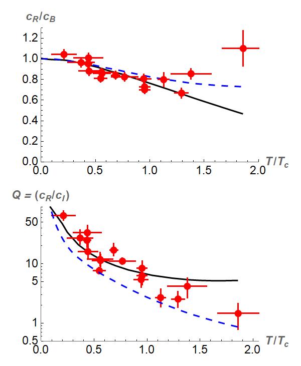
Figure 1: Results from numerical solution of the dispersion equation $u_{0}=c_{R}-ic_{I}$ vs temperature in the 2D case. Upper panel: the normalized speed of sound $c_{R}/c_{B}$ as a function of the normalized temperature $T/T_{c}$, where $c_{B}=\sqrt{gn_{0}/m}$ is the Bogoliubov velocity, $T_{c}=2\pi\hbar^{2}n_{0}/(mk_{B}\ln{(380\ \hbar^{2}/(mg))})$ is the Berezinskii-Kosterlitz-Thouless critical temperature, and $n_{0}$ is the 2D number density at equilibrium. Lower panel: $Q=c_{R}/c_{I}$ quality factor of the sound damping. To compare the two transport theories with the experiment of Ref. ville2018 we choose $g=0.16\ \hbar^{2}/m$. The blue dashed curve is the result of the Vlasov-Landau theory; the black solid curve the result of the Andreev–Khalatnikov theory. Red dots are measured data of Ref. ville2018 .

In the upper panel of Fig. 1 we plot the real part of the scaled speed of sound $c_{R}/c_{B}$, with $c_{B}=\sqrt{gn_{0}/m}$ the Bogoliubov sound velocity. Remarkably, the experimental data (filled circles) are very well reproduced, both below and above $T_{c}$, by the Vlasov-Landau equation (dashed curve) but also by the Andreev-Khalatnikov equations (solid curve). At very low temperature $T$ the two curves of the two theories practically superimpose. In the lower panel of Fig. 1 there is instead the quality factor $Q=c_{R}/c_{I}$ of the sound damping, namely the ratio between the real and the imaginary part of the sound velocity $u_{0}=c_{R}-ic_{I}$. For this quality factor $Q$, the Andreev-Khalatnikov theory (solid curve) is in much better agreement with the experimental results (filled circles) with respect to the Vlasov-Landau theory (dashed curve) up to the critical temperature $T_{c}$. Above the critical temperature $T_{c}$ it seems that the quality factor $Q$ can be better reproduced by the Vlasov-Landau equation. Notice that in 2D the damping of the collisionless mode was investigated also in Ref. indy by using a time-dependent Hartree-Fock-Bogoliubov approach, which practically gives the same results of the linearized Vlasov-Landau equation ota2018 ; lipparini .

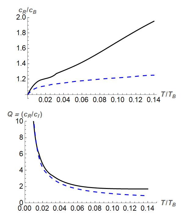
Figure 2: Results from numerical solution of the dispersion equation $u_{0}=c_{R}-ic_{I}$ versus temperature in the 1D case. Upper panel: the normalized speed of sound $c_{R}/c_{B}$ as a function of the normalized temperature $T/T_{B}$, where $c_{B}=\sqrt{gn_{0}/m}$ is the Bogobliubov velocity, $T_{B}=2\pi n_{0}^{2}\hbar^{2}/(mk_{B})$ is the degeneration temperature, and $n_{0}$ the 1D number density at equilibrium. We choose $g=0.16\ \hbar^{2}n_{0}/m$. Lower panel: $Q$ quality factor of the sound damping: $Q=c_{R}/c_{I}$. The blue dashed curve is the result of the Vlasov-Landau theory; the black solid curve is obtained using the Andreev-Khalatnikov theory.

We investigate also the 1D weakly-interacting Bose gas in the collisionless regime. Unfortunately there are not yet available experimental data in this configuration. Thus, our 1D predictions can be a strong benchmark for next future experiments and also for forthcoming theoretical investigations. Strictly speaking, in the thermodynamic limit and with $T>0$, for a 1D weakly-interacting Bose gas there is neither Bose-Einstein condensation nor superfluidity pitaevskii1991 ; super-book ; stoof . However, a finite 1D system of spatial size $L$ is effectively superfluid if $k_{B}T\ll E_{\phi}/\ln{(L/\xi)}$, where $E_{\phi}\simeq\hbar^{2}n_{0}/(m\xi)$ is the energy needed to create a phase slip (topological defect, also known as black soliton) and $\xi=\hbar/\sqrt{2mgn_{0}}$ is the healing length super-book .

In Fig. 2 we show our numerical results for the complex speed of sound $u_{0}=c_{R}-ic_{I}$ of the 1D bosonic system obtained by solving the Vlasov-Landau equation (dashed curves) and the Andreev-Khalatnikov equations (solid curves). The quantities are plotted as a function of the scaled temperature $T/T_{B}$ where $T_{B}=2\pi n_{0}^{2}\hbar^{2}/(mk_{B})$ is the temperature of Bose degeneracy, where the 1D thermal de Broglie wavelength $\lambda_{T}=\hbar\sqrt{2\pi/(mk_{B}T)}$ becomes equal to the average distance $n_{0}^{-1}$ between bosons, with $n_{0}$ the equilibrium 1D number density. As clearly reported in the upper panel of Fig. 2, contrary to the 2D case, in 1D the real part $c_{R}$ of the sound velocity $u_{0}$ increases by increasing the temperature $T$. However, the Andreev-Khalatnikov theory predicts a much larger slope. Indeed, this suggests that in 1D the determination of this slope can be experimentally use to the determine the superfluid nature of the Bose gas. We have also found that, while in 2D the isothermal velocity $c_{T}$ of Eq. (19) at low temperature is close to the real part of $u_{0}$ obtained by solving Eq. (18), in the 1D system this is not the case.

In the lower panel we plot the quality factor $Q=c_{s}/c_{I}$ of the sound damping: the two theoretical curves are very close each other. This result implies that in 1D the damping is not very useful to discriminate between the two transport theories.

It is important to stress that marked differences shown in Figs. 1 and 2 are also due to the fact that the scaled temperature is in units of $T_{c}$ in 2D and in units of $T_{B}$ in 1D. A quite complicated analytical expression for the sound velocity $u_{0}$ of the Vlasov-Landau equation (2) can be derived if $f_{0}(p)\simeq k_{B}T/(p^{2}/2m-{\tilde{\mu}})$, i.e. under the condition $|{\tilde{\mu}}|\ll k_{B}T\ll k_{B}T_{B}$. In this way, in 2D one finds ota2018 ; cappellaro2018 that the real part of $u_{0}$ decreases by increasing in the temperature $T$, while in 1D we obtain the opposite, in very good agreement with our numerical results. As discussed in Appendix A, the 2D Vlasov-Landau equation can be reduced to an effective 1D equation but with an effective 1D Bose-Einstein distribution which is quite different with respect the one of the strictly 1D case. Clearly, the behavior of $u_{0}$ vs $T$ crucially depends on the considered Bose-Einstein distribution.

V Conclusions

We have analyzed the collisionless sound mode of a 2D weakly-interacting bosonic fluid, where recent experimental data are available ville2018 , but also the collisionless sound mode of the 1D bosonic fluid, where experimental data are not yet available. We have compared two theories: the Vlasov-Landau equation versus the Andreev-Khalatnikov equations. The Andreev-Khalatnikov equations are more sophisticated because, contrary to the Vlasov-Landau equation, they also take into account the presence of a superfluid velocity. Our 2D theoretical results, also confronted with the experimental data, strongly suggest that below the critical temperature of the superfluid-to-normal transition the bosonic fluid is better described by the Andreev-Khalatnikov theory, while above the critical temperature the Vlasov-Landau theory seems more reliable. For the collisionless 1D Bose gas, our calculations show that the real part of the sound velocity grows by increasing the temperature and its slope determines the superfluid nature of the system. This prediction, as well as the reduction of sound damping due to the superfluid velocity, can be very useful for forthcoming theoretical and experimental investigations of collisionless superfluids.

Appendix A

In the linearized Vlasov-Landau equation (5) there is the relevant quantity

$$\int d^{D}{\bf p}{{\nabla_{p}f_{0}}\cdot{\bf n}\over{\bf p}\cdot{\bf n}-u_{0}}$$ (23)

By chosing ${\bf n}$ parallel to x-axis, this expressione simplifies to

$$\int d^{D}{\bf p}{\partial_{p_{x}}f_{0}\over p_{x}-u_{0}}$$ (24)

In dimension $D=2$ it is straightforward to note that

$$\int d^{2}{\bf p}{\partial_{p_{x}}f_{0}\over p_{x}-u_{0}}=\int dp_{x}\partial_{p_{x}}\left(\int dp_{y}f_{0}\right){1\over p_{x}-u_{0}}$$ (25)

Thus, both in dimension one and two, ultimately one has to deal with one-dimensional integrals. The integral operator comes from an inverse Laplace transform, hence the path of integration is defined in the complex $p$-plane. The recipe for choosing the right path was given by Landau landau46 , and may be found in several recent references, e.g., baldovin ; nicholson . Here we provide just the results. The integral (25) writes as the sum of an integral along the real axis plus a contribution coming from poles in the complex plane:

$$\int_{\infty}^{+\infty}dp_{x}\partial_{p_{x}}\left(\int dp_{y}f_{0}\right){1\over p_{x}-u_{0}}+{\cal J}$$ (26)

If $Im(u_{0})>0$ then ${\cal J}=0$. Conversely, if $Im(u_{0})<0$ we have

$${\cal J}=2\pi i\,\partial_{p_{x}}f_{x}(p_{x}=u_{0})$$ (27)

with

$$f_{x}(p_{x})=\int dp_{y}\,p_{y}\ f_{0}(p_{x},p_{y})$$ (28)

Appendix B

In the Andreev-Khalatnikov theory one has to deal with several integrals of the kind

$$\int dp{F(p)\over\partial_{p}E(p)-u_{0}}$$ (29)

where we have dropped the $x$ lowerscript for convenience. $F(p)$ is one of the functions appearing in Eq. (22). Since $E(p)$, as defined in (11), is a nonlinear function of $p$, the recipe of Eqns. (26,27) needs some modifications. Let ${\bar{p}}$ be a root of the function

$${\cal D}(p)=\partial_{p}E(p)-u_{0}:{\cal D}({\bar{p}})=0$$ (30)

namely

$${\cal D}({\bar{p}})=0$$ (31)

Then, we may expand ${\cal D}(p)$ around $p={\bar{p}}$:

$${\cal D}\simeq(p-{\bar{p}})\partial_{p}^{2}E({\bar{p}})$$ (32)

Ultimately, therefore, the integrals (29) are evaluated as

$$\int dp{F(p)\over\partial_{p}E(p)-u_{0}}=\int_{-\infty}^{+\infty}dp{F(p)\over\partial_{p}E-u_{0}}+{\cal J^{\prime}}$$ (33)

This time we get

$${\cal J^{\prime}}=2\pi i{F({\bar{p}})\over\partial_{p}^{2}E({\bar{p}})},\quad Im({\bar{p}})<0$$ (34)

References

- (1) L.D. Landau, J. Phys. USSR 5, 71 (1941).
- (2) F. London and H. London, Proc. Royal Soc. A 149, 866 (1935).
- (3) L. Tisza, Nature 141, 913 (1938).
- (4) L.D. Landau and E.M. Lifshitz, Fluid Mechanics, vol. 6 of Course of Theoretical Physics (Pergamon Press, 1987)
- (5) I.M. Khalatnikov, An Introduction to the Theory of Superfluidity (Pergamon Press, 1965).
- (6) A. Schmitt, Introduction to Superfluidity. Field-Theoretical Approach and Applications (Springer, 2014).
- (7) A. Andreeev and I.M. Khalatnikov, Sov. Phys. JEPT 17, 1384 (1963).
- (8) L.D. Landau and E.M. Lifshitz, Physical Kinetics, vol. 10 of Course of Theoretical Physics (Butterworth-Heinemann, 1981).
- (9) W.M. Whitney and C.E. Chase, Phys. Rev. Lett. 9, 243 (1962).
- (10) D.R. Nicholson, Introduction to plasma theory, cap. 6 (Wiley, 1983).
- (11) J.L. Ville, R. Saint-Jalm, E. Le Cerf, M. Aidelsburger, S. Nascimbene, J. Dalibard, and J. Beugnon, Phys. Rev. Lett. 121, 145301 (2018).
- (12) M. Ota, F. Larcher, F. Dalfovo, L. Pitaevskii, N.P. Proukakis, and S. Stringari, Phys. Rev. Lett. 121, 145302 (2018).
- (13) A. Cappellaro, F. Toigo, and L. Salasnich, Phys. Rev. A 98, 043605 (2018).
- (14) A. Vlasov, J. Phys. (Moscow) 9, 25 (1946).
- (15) L.D. Landau, J. Phys. (USSR) 11, 23 (1947).
- (16) E. Lipparini, Modern Many-Particle Physics (World Scientific, 2008).
- (17) Z. Wu, S. Zhang, and H. Zhai, Phys. Rev. A 102, 043311 (2020).
- (18) V. L. Berezinskii, Sov. Phys. JETP 34, 610 (1972).
- (19) J. M. Kosterlitz and D. J. Thouless, J. Phys. C: Solid State Phys. 6, 1181 (1973).
- (20) L. Pitaevskii and S. Stringari, J. Low Temp. Phys. 85, 377 (1991).
- (21) B. Svistunov, E. Babaev, and N. Prokof’ev, Superfluid States of Matter (CRC Press, Boca Raton, 2015).
- (22) N. Prokof’ev, O. Ruebenacker and B. Svistunov, Phys. Rev. Lett. 87, 270402 (2001).
- (23) N. Prokof’ev, O. Ruebenacker, and B. Svistunov, Phys. Rev. A 66, 043608 (2002).
- (24) F. Baldovin, A. Cappellaro, E. Orlandini, and L. Salasnich, J. Stat. Mech. 063303 (2016).
- (25) N. Bogoliubov, J. Phys. (USSR) 11, 23 (1947).
- (26) J.O.Andersen, U. Al Khawaja, and H. T. C. Stoof, Phys. Rev. Lett. 88, 070407 (2002).
- (27) H.T.C. Stoof, K.B. Gubbels, and D.B.M. Dickerscheid, Ultracold Quantum Fluids (Springer, 2009).
- (28) M.-C. Chung and A.B. Bhattacherjee, New J. Phys. 11, 123012 (2009).